Download s - Bison Academy

NDSU
8: Frequency Domain Techniquess
ECE 461
Gain Compensation Using a Nyquist Plot
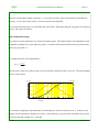
On a Nyquist plot
The X-axis plots real(G(jw))
The Y axis plots imag(G(jw)).
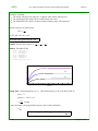
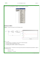
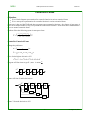
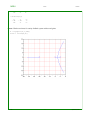
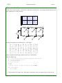
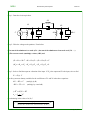
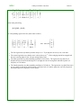
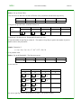
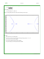
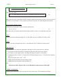
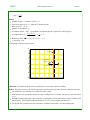
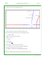
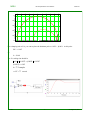
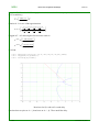
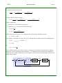
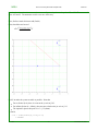
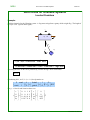
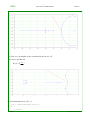
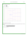
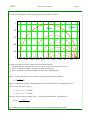
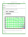
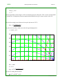
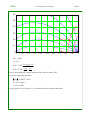
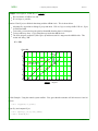
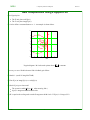
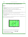
M-circles define a constant distance to -1. An example is shown below.
2
0dB
3dB
1
6dB
9dB
12dB
0
-1
-1
-2
-3
-2
-1
real
0
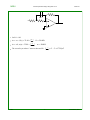
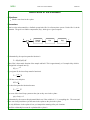
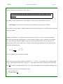
Nyquist diagram. M-circles mark points where
1
G
1+G
= constant.
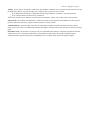
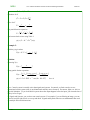
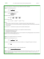
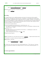
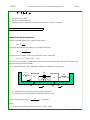
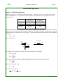
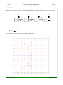
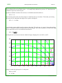
Two ways to use a Nichols chart to find a feedback gain follow:
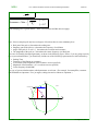
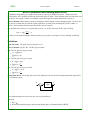
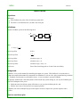
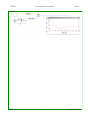
Method #1: (useful if using MATLAB)
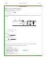
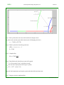
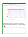
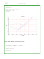
i) Plot G(jw) as imag(G(jw)) vs. real(G(jw)).
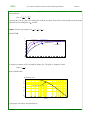
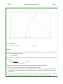
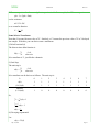
ii) Scale G(jw) up or down until
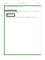
The system is stable ( G(jω) < 1 when crossing 1800.)
G(jω) is tangent to the desired M-circle.
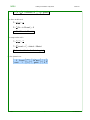
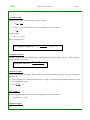
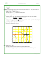
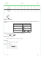
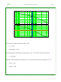
iii) K is equal to the scaling used to make G tangent to the M-circle. If G(jw) is 2x larger, K=2.
JSG
1
rev 02/27/02