Download Rural HSPF modelling Technical Guide

Rural HSPF modelling
Technical Guide
Dr Andrew Phillips
Catchment Science Centre
University of Sheffield
Contents
1
Introduction
1
2
2.1
2.2
Data and Software Requirements
Data required
Software required
1
1
2
3
3.1
3.2
3.2.1
3.2.2
3.3
3.3.1
3.3.2
3.4
3.5
3.5.1
3.5.2
3.6
Preliminary Model Data Preparation
Model catchment(s)
Model sub-catchment delineation (Topography)
Basins method
Arc Hydro Tools Method (Manual)
Met data – Part 1
Precipitation
Potential Evapotranspiration
Land Use – Part 1
Met data – Part 2
Import data into WDM file (precipitation and evapotranspiration)
Potential Evapotranspiration
Land Use – Part 2
3
3
3
3
5
11
11
13
14
16
16
18
20
4
4.1
4.2
4.2.1
4.2.2
Model Input File Creation
Basins method
Arc Hydro Tools Method (Manual)
GIS processing
HSPF Input File Formatting
21
21
23
23
26
5
5.1
5.2
5.3
5.4
5.5
5.5.1
5.5.2
5.5.3
5.6
Create HSPF Model (Part 1 - Hydrological)
Create HSPF Project
Define Initial Met Segment
WinHSPF GUI
Set Model Simulation Time and Met Segments
Change Hydrological Parameters
HSPF Hydrological Parameters
Editing Parameters within WinHSPF
Editing Parameters Directly in the .uci File
Add Model Flow Output
30
30
31
32
33
36
36
36
38
39
6
6.1
6.1.1
6.1.2
6.1.3
6.1.4
6.1.5
6.2
6.2.1
FIO
Bacteria Indicator Tool
Sub-catchments
Land Use
Animal numbers (agcensus)
Manure Application Practices
Conversion of accumulation values
Point Sources
Add to Point Source to .wsd
42
42
42
42
43
48
48
49
49
7
7.1
7.2
Create HSPF Model (Part 2 – FIO)
Add Pollutant
Edit Control Cards
52
52
52
7.3
7.4
7.5
7.6
Edit Properties and Enter Accumulations from the BIT
Add Monthly Accumulation Rates and Limiting Storage Values from BIT
Add Point Sources
Add Model Water Quality (Faecal Coliform) Output
53
55
59
60
8
Running the Model
63
9
9.1
9.2
9.3
9.4
9.5
Common Model Errors
Issues with input Met data
Data conversion
FTABLES
Errors when using BASINS to delineate sub-catchments
Getting additional help
64
64
64
64
65
65
10
10.1
10.2
Outputting Model Results
Viewing Model Results
Exporting Model Output Data
66
66
67
11
11.1
11.1.1
11.1.2
11.2
11.2.1
11.2.2
11.2.3
Calibration
Hydrological Calibration
Interactive and Automated Hydrological Calibration
Flow Data Conversion
FIO calibration
BIT calibration
FIO Decay rate
FIO Data Conversion
70
70
70
70
71
71
71
72
12
12.1
12.1.1
12.1.2
12.1.3
12.2
12.2.1
12.2.2
Model Changes for Scenario Modelling
Management Scenarios
BIT spreadsheet changes
Urban Point Source Changes
Land Use Changes
Climate Scenarios
Generating New Met Data
Modifying Existing Met Data
73
73
73
73
74
74
74
75
Appendices
Appendix A – ArcMap Model Builder Diagrams for .ptf and .rch HSPF Input
Files
Appendix B – ArcMap Model Builder Diagrams for .wsd HSPF Input File
Appendix C – .psr File Example
Appendix D – .ptf File Example
Appendix E – .rch File Example
Appendix F – .wsd File Example
Appendix G – .uci File Example
Appendix H – Additional Resources
77
77
80
84
85
86
87
89
101
1. Introduction
This document serves as a technical guide for the processing of data, model operation and
exporting of results from the Hydrological Simulation Program – Fortran (HSPF) model
which has been used in WP2 (diffuse rural modelling) of the Cloud To Coast project.
The document has been written in process order, and details the steps required to prepare
and operate the model in the required sequence for a user starting the process from
scratch. These steps detail the data and software required for the modelling process, the
preparation of the data for use in the HSPF model, the creation and configuration of the
HSPF model, running the model and outputting model results. Additional resources are also
signposted (and included in Appendix H), which provide further information and detail.
If pre-prepared models are being used, the initial steps will explain their construction.
Potential modifications and alterations to the model, for example in exploring management
or climate change scenarios are possible using the existing models, and steps to accomplish
this are detailed in later sections of this document.
2. Data and Software Requirements
2.1 Data required
Dataset
Use
Source
DEM
Watershed delineation and
topographic parameters
EDINA Digimap: Ordnance
Survey Collection
River Network
Used to burn into DEM for additional
hydrologic accuracy (optional)
CEH
Precipitation data
(EA rain gauge)
Time series rainfall data (including
locations)
Environment Agency
Potential
Evapotranspiration
(MORECS)
Time series potential
evapotranspiration data (including
locations)
United Utilities
Land Use Data (Land
Cover Map 2007)
Information on land use.
EDINA Digimap:
Environment Collection
Agricultural
information
(agcensus Livestock numbers)
Data to quantify grazing numbers in
sub-catchments
EDINA
River flow data
Calibration of modelled flow output
Environment Agency
Calibration of Faecal Coliform output
C2C project field work
(EA flow gauge)
FIO water quality
data
Table 1.1: Data Required
1
2.2 Software required
Software
Notes
Source
BASINS
(including
WinHSPF)
Provided by U.S. EPA. Test version may
solve any compatibility issues.
http://water.epa.gov/scitech/datait/
models/basins/download.cfm
(stable release)
http://www.aquaterra.com/resourc
es/downloads/basins4.php
(test version)
WDMUtil/
Maybe included with BASINS but also
available as a standalone package,
which may be more convenient.
http://www.aquaterra.com/resourc
es/downloads/basins4.php
ESRI ArcGIS
Desktop
(ArcMap)
The GIS package used for this project
and guide.
Commercial software
Arc Hydro
Tools
Geoprocessing toolset for GIS
software.
https://mft.esri.com/ (FTP site)
GenScn
Login and password for ftp site, as
well as further instruction and
tutorials can be found from the Arc
Hydro forum:
http://forums.arcgis.com/forums/88Arc-Hydro
MS Excel
Spreadsheet software
Commercial software
MS Notepad
Text editor software
Commercial software (provided
with windows)
Table 2.1: Software Required
2
3. Preliminary Model Data Preparation
3.1 Model catchment(s)
Reason: Define outer boundaries for model limits. This is based on the rivers being modelled
and where they drain. In the case of C2C the model extent and the rivers to be modelled had
been identified by the strategic partners. The locations where the rural HSPF modelled
drained into the river/estuary model created additional points within this larger catchment
that defined the boundaries of the rural HSPF models.

Use GIS to calculate a watershed from a DEM based on the rivers to be modelled and/or
the points to be drained to.
3.2 Model sub-catchment delineation (Topography)
Reason: To create model sub-catchments (the spatial units used to define and configure the
model) within the overall model catchment(s) and calculate topographic parameters for
these (slope, area, and channel length).
Two methods were used to delineate the watersheds. One using the U.S. EPA BASINS
software which is packaged together with the HSPF model. In some cases the watershed
delineation using this software was problematic and did not produce acceptable catchments.
Predominantly these were smaller, lower-level catchments which were topographically more
homogenous. In these instances a manual method was undertaken using Arc Hydro Tools for
ArcGIS and tools within ArcGIS itself to process and delineate the required watersheds.
Small model catchments which comprised only a single sub-catchments were also processed
using the manual Arc Hydro method.
Both methods are outlined below.
3.2.1 Basins method






Open BASINS software
Create New Project
Without selecting any features, click Build
Click Yes to dismiss the Data Extraction message.
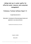
Save the project in an appropriate directory
Enter Projection Properties as shown in figure 3.1 – these match GB National Grid.
3
Figure 3.1: BASINS Projection Properties

Use the Add data button (figure 3.2) to add data
Figure 3.2: BASINS Add Data Button

Add:
o
o
o


DEM
Model catchment shapefile
Rivers shapefile
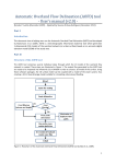
On the top menu options, go to Watershed Delineation>Automatic
Fill out the form as in figure 3.3, with the exception of # of cells – leave that as the value
set by the BASINS software.
4
Figure 3.3: BASINS Automatic Watershed Delineation





Check Advanced Settings for more options if you wish
Click Run All
Note: If errors occur in the processing of the sub-catchments, either software based
(with error message windows) or in the shape of the expected sub-catchment
delineations (e.g. areas for the model catchment not covered by sub-catchments) then
inspect the DEM and consider using the Arc Hydro (manual method instead).
Locate the created Watershed Shapefile (demw.shp) and Stream Reach Shapefile
(demnet.shp). These should be saved in the same directory in which your BASINS
project was saved. Take a copy of these shapefiles.
Save BASINS project for later use in preparing the model input files (Model Input File
Creation>BASINS method)
3.2.2 Arc Hydro Tools Method (Manual)
Sub-catchment delineation can also be performed in ArcGIS using Arc Hydro Tools, which
are a set of geoprocessing tools designed to support water resource applications. Using Arc
Hydro Tools to delineate the sub-catchments allows a greater amount of user control over
the delineation and processing of the sub-catchments. It also allows for the processing of
individual sub-catchments for smaller catchment models. The disadvantage of using Arc
Hydro Tools and ArcGIS over BASINS is that more manual processing is required to prepare
the data into the correct format for entry into the HSPF model. The below method requires
ArcGIS complete with the Spatial Analyst extension and Arc Hydro Tools to be installed and
activated.
The initial step involves processing the DEM. This can be done once for a DEM that covers the
entire C2C area before further processing the individual model catchments.
5




Open ArcGIS ArcMap and open the Arc Hydro Tools toolbar by right-clicking in an empty
section of the toolbar and selecting Arc Hydro Tools
Add to ArcMap:
o DEM
o Rivers shapefile
Save the ArcMap document (a .mxd file). Arc Hydro Tools will save output files in the
same directory as the .mxd file.
Create a reconditioned DEM by burning-in the channel outline from the Rivers file:
o Click Terrain Preprocessing on the Arc Hydro Tools Toolbar
o In the menu that drops down go to DEM Manipulation>DEM Reconditioning
(figure 3.4).
Figure 3.4: Arc Hydro Tools Toolbar



Select the DEM for the Raw DEM
Select the Rivers shapefile for the Agree Stream
Leave other fields as their default values, as in figure 3.5.
6
Figure 3.5 Arc Hydro Tools – DEM Reconditioning


Click OK
Fill sinks
o Click Terrain Preprocessing on the Arc Hydro Tools Toolbar
o In the menu that drops down go to DEM Manipulation>Fill Sinks
o Select the newly created AgreeDEM as the DEM and fill out the rest of the details
as in figure 3.6.
Figure 3.6 Arc Hydro Tools – Fill Sinks

Click OK
7
Having prepared a DEM for the entire C2C area, the model sub-catchments can be
processed individually for better speed and error checking. This process will need to be
completed for each of the model catchments to be run.




Open a new ArcMap document
Add to ArcMap:
o The Filled DEM (Fil) which was created in the previous step.
o A model catchment shapefile
Save the ArcMap document (a .mxd file). Arc Hydro Tools will save output files in the
same directory as the .mxd file. This .mxd document will be specific to the one model
(the model represented by the loaded catchment shapefile).
Calculate Flow Direction
o Click Terrain Preprocessing on the Arc Hydro Tools Toolbar
o In the menu that drops select Flow Direction
o Enter Fil (the filled DEM) as the Hydro DEM
o Enter the model catchment as the Outer Wall Polygon
o Leave the remaining options as in figure 3.7.
Figure 3.7: Arc Hydro Tools – Flow Direction

Click OK

Calculate Flow accumulation
o Click Terrain Preprocessing on the Arc Hydro Tools Toolbar
o In the menu that drops select Flow Accumulation
o Check that the details are entered correctly as in figure 3.8.
Figure 3.8: Arc Hydro Tools – Flow Accumulation

Click OK
8

Create Stream Definition
o Click Terrain Preprocessing on the Arc Hydro Tools Toolbar
o In the menu that drops select Stream Definition
o Enter the Number of cells as 20000 (used for single sub-catchment or small size
model catchments) or the use the BASINS cell threshold (for erroneous BASIN
outputs) if the cell threshold is greater than 20000. The BASINS cell threshold is
given as the # of cells value when attempting Automatic Watershed Delineation
(see section 3.2.1).
o Check that the details are entered correctly as in figure 3.9.
Figure 3.9: Arc Hydro Tools – Stream Definition

Click OK

Create Stream Segmentation
o Click Terrain Preprocessing on the Arc Hydro Tools Toolbar
o In the menu that drops select Stream Definition
o Check that the details are entered correctly as in figure 3.10.
Figure 3.10: Arc Hydro Tools – Stream Segmentation

Click OK
9

Perform Catchment Grid Delineation
o Click Terrain Preprocessing on the Arc Hydro Tools Toolbar
o In the menu that drops select Catchment Grid Delineation
o Check that the details are entered correctly as in figure 3.11.
Figure 3.11: Arc Hydro Tools – Catchment Grid Delineation

Click OK

Perform Catchment Polygon Processing
o Click Terrain Preprocessing on the Arc Hydro Tools Toolbar
o In the menu that drops select Catchment Polygon Processing
o Check that the details are entered correctly as in figure 3.12.
Figure 3.12: Arc Hydro Tools – Catchment Polygon Processing

Click OK

Perform Drainage Line Processing
o Click Terrain Preprocessing on the Arc Hydro Tools Toolbar
o In the menu that drops select Drainage Line Processing
o Check that the details are entered correctly as in figure 3.13.
10
Figure 3.13: Arc Hydro – Drainage Line Processing

Click OK


Save the .mxd to include a reference of the processing for the catchment.
Right-click each of the following in the table of contents window and using Data>Export
Data… Save a copy of them as shapefiles:
o DrainageLine
o Catchment
Close ArcMap.

The DrainageLine and Catchment shapefiles are used in the calculation of topographic values
that represent the model sub-catchments. The Catchment shapefile identifies the delineated
HSPF sub-catchments and their areas, the DrainageLine shapefile stores the representative
channel or reach of each sub-catchment and the sub-catchment downstream flow order.
3.3 Met data – Part 1
The met data (precipitation and potential evapotranspiration) that is required to drive the
hydrological component of the HSPF model needs to be pre-prepared. The data needs to be
inspected for errors and repaired with as much accuracy as possible. The data also needs to
be converted into the required model time steps and measurement units as well as being
formatted correctly to facilitate entry into the .wdm (Watershed Data Management) format
in which the data is stored for use with the HSPF model. Location data marking where the
data was collected from also needs to be recorded.
The processing steps outlined in this section can be undertaken using MS Excel.
3.3.1 Precipitation

Conversion to inches from m3s-1.
Reason: Model is run using imperial units.
o

Multiply mm by 0.0393700787 to get inches.
Fill-in missing data:
Reason: To create a complete time-series of precipitation data
11
o
o
o
o
o
o
o

Gauge data checked for number of missing/error values (comments can record
why data is missing)
If count of missing cells is over 100 they are substituted with data from the closest
neighbouring rain gauge.
Gauge data rechecked for missing/error values
If count of missing cells remains over 100 they are substituted with data from the
second closest neighbouring rain gauge.
Process is repeated until count of missing cells is less than 100 (or if neighbouring
stations become too far away to be broadly comparable).
Any remaining cells are assigned a value of 0, following an inspection to check that
appears sensible within the time series.
Cleaned, interpolated rainfall series is saved as a new file.
Convert 15 min data into hourly
Reason: Model will run in hourly time-steps. All input data will need to be in the same time
units. If they differ the model will not run correctly.
o
Calculate the sum of 4, 15 minute precipitation cells so that the precipitation at
XX:00 = the sum of the precipitation at that time and the 3 values prior to it.
Figure 3.14 demonstrates an example of this.
Time
XX:15
XX:30
XX:45
XX:00
Precipitation
=sum(XX:15, XX:30, XX:45, XX:00)
Figure 3.14: MS Excel – Conversion to Hourly Time-Steps
o

Clean the data so that only the hourly summed values remain (with date and
time).
Save precipitation data in correct format for importing into .wdm
Reason: Saving the data following the template provided below and as a .csv format allows
for relatively simple import into a .wdm file using WDMUtil. This is the format used to store
time-series data in by HSPF.
o
Value
Prepare the data in the column format illustrated in figure 3.15.
Year
Month
Day
Hour
Minute
Figure 3.15: MS Excel – Precipitation Data Column Format
o
o

Remove any header row
Save the data as a .csv file
Rain gauge location
Reason: Rain gauge station locations are needed by HSPF when saving the data within a .wdm
file and when selecting an initial met station and assigning met segments (section 5.4) when
creating an HSPF model. Coordinates need to be recorded as latitude and longitude in
12
decimal degrees for .wdm file entry. Additionally rain gauge locations are used to determine
which rain gauge data should be used for each model sub-catchment according to proximity.
o
o
o
o
o
o
Plot OS Nation Grid coordinates of rain gauges using GIS (grid references
available in station header information)
Convert OS National Grid References into latitude and longitude in decimal
degrees (WGS84 format) and record for later use when storing data in .wdm file.
Create Thiessen Polygon layer (using ArcMap) to create polygons representing
the area of influence for each rain gauge based on Euclidean geometry.
Use GIS to perform a spatial Join on the model sub-catchments with the rain
gauge locations so that each sub-catchment is assigned the rain gauge which falls
within it or the gauge which is closest to it.
Can visually check the spatial join using Thiessen Polygon layer created previously.
This data can be used to assign an initial model met segment (section 5.1 and 5.2)
and to add and assign met segments for all model operations when creating the
HSPF model (see section 5.4).
3.3.2 Potential Evapotranspiration

MORECS values come in a weekly time series.
Reason: Model will run in hourly time-steps. All input data will need to be in the same time
units. If they differ the model will not run correctly. A complete time-series of
evapotranspiration data is also required.
o

Use linear interpolation to compute daily values from the weekly data within a
spreadsheet.
Data should be converted from mm to inches.
Reason: Model is run using imperial units.
o

Multiply mm by 0.0393700787 to get inches.
Save potential evapotranspiration data in correct format for importing into .wdm
Reason: Saving the data following the template provided below and as a .csv format allows
for relatively simple import into a .wdm file using WDMUtil. This is the format used to store
time-series data in by HSPF.
o
Value
Prepare the data in the column format illustrated in figure 3.16.
Year
Month
Day
Hour
Minute
Figure 3.16: MS Excel – Potential Evapotranspiration Data Column Format
o
o

Remove any header row
Save the data as a .csv file
An additional step is required to disaggregate the evapotranspiration from a daily timestep into an hourly one. This is undertaken in the WDMUtil software once the
evapotranspiration data has been imported.
13
3.4 Land Use – Part 1
The Land Cover Map (LCM2007) data from CEH has more categories than is ideal for
modelling in HSPF. A greater number of categories causes a greater level of model
complexity which can lead to a greater chance of errors. Simplifying the categories to land
uses of relevance will aid the modelling process.
Should changes in land use categories be required they can be made by repeating this
process and rebuilding the model. Having reclassified the land cover map into a HSPF land
use layer this file can then be used by BASINS or through manual processing to build the
model input files.
The processing of the land use date can be achieved using ArcMap using the following steps.







Convert the downloaded LCM2007 data from raster format to a vector shapefile in
ArcMap
A lookup table is provided (Table 3.1) which enables the LCM2007 GridCode values to be
linked with the relevant LCM2007 classification and the HSPF land use categories.
Save the lookup table as a table (an Excel workbook is suitable)
In ArcMap load the lookup table
Join the lookup table to the converted LCM2007 shapefile using the GridCode values
Save the joined output allowing you to reclassify LCM2007 land use categories into HSPF
land use categories
Merge polygons based on HSPF land use category and save output.
14
GridCode LCM2007Class
0
Unclassified
1
Broadleaved, mixed and yew
woodland
2
Coniferous woodland
3
Arable and horticulture
4
5
6
7
8
9
Improved grassland
Rough grassland
Neutral grassland
Calcareous grassland
Acid grassland
Fen, marsh and swamp
10
Heather
11
Heather grassland
12
Bog
13
Montane habitats
14
Inland rock
15
16
17
18
19
20
21
22
23
Saltwater
Freshwater
Supra-littoral rock
Supra-littoral sediment
Littoral rock
Littoral sediment
Saltmarsh
Urban
Suburban
HSPFLandUse
Unclassified
Woodland
Woodland
Arable &
horticultural
Grassland
Grassland
Grassland
Grassland
Grassland
Mountain, heath,
bog
Mountain, heath,
bog
Mountain, heath,
bog
Mountain, heath,
bog
Mountain, heath,
bog
Mountain, heath,
bog
Coast, Sea
Water
Coast, Sea
Coast, Sea
Coast, Sea
Coast, Sea
Coast, Sea
Built-up areas
Built-up areas
Table 3.1: Land use Lookup - LCM2007 land use categories to HSPF land use categories.
15
3.5 Met data – Part 2
3.5.1 Import data into WDM file (precipitation and evapotranspiration)
Reason: .wdm (Watershed Data Management) files are the format in which HSPF stores input
and output time series data. Input time series data includes the precipitation and
evapotranspiration data. Having prepared the data in the way described above the saved .csv
files can be imported into a .wdm file using the WDMUtil software. The import steps below
are the same regardless of data-type unless otherwise stated.
















Open WDMUtil
Create a new .wdm file (File>New) or open an existing .wdm file (File>Open)
Select File>Import
Locate a saved Met data .csv file
Optionally create a template for input or select a previously created template (this can
save time) or select Blank Script and Click Edit
Uncheck the Skip option under Header
Check Character: under Column Format and check that a , [comma] is entered
Check that the data is displayed correctly in the preview – similar to figure 3.17.
Open WDMUtil
Create a new .wdm file (File>New) or open an existing .wdm file (File>Open)
Select File>Import
Locate a saved Met data .csv file
Optionally create a template for input or select a previously created template (this can
save time) or select Blank Script and Click Edit
Uncheck the Skip option under Header
Check Character: under Column Format and check that a , [comma] is entered
Check that the data is displayed correctly in the preview – similar to figure 3.17.
Figure 3.17: WDMUtil – Import Script Creation

Click the Data Mapping Tab
16

Enter the values in the input column as shown in figure 3.18.
Figure 3.18 WDMUtil – Import Script Creation – Data Mapping



Click Read Data
Double-click on new time series entry to open the Edit Time Series Attributes window
and allow editing of the attributes.
Add the attributes in table 3.2 according to the dataset and data type you are importing:
Attribute
Precipitation Data
Scenario
Location
OBSERVED
(Name of location – 8
characters)
PREC
(Description of
location/data)
(Latitude)
(Longitude)
Constituent
Description
LATDEG
LNGDEG
Potential
Evapotranspiration Data
OBSERVED
(Name of location – 8
characters)
EVAP
(Description of
location/data)
(not required)
(not required)
Table 3.2: WDMUtil – Time Series Attributes Entry (Capitalised text indicates default text
entry, descriptions in brackets indicate user determined value that needs to be entered)

The LATDEG and LNGDEG attributes for precipitation data will need to be added
manually before entering coordinates.
o In the Edit Time Series Attributes window click Add Attributes
o Scroll down to the new attribute row, left click in the empty attribute cell and
enter the attribute name (LATDEG or LNGDEG)
o Enter the corresponding coordinate in the DSN1 field.
o Repeat the process for the other coordinate.

An example of a completed Edit Time Series Attribute window for precipitation data is
shown in figure 3.19.
17
Figure 3.19: WDMUtil – Time Series Attributes


Click OK
Click the Write Time Series to WDM button (outlined in red in figure 3.20)
Figure 3.20: WDMUtil – Write Time Series Tool
o
o
In the Write to WDM dialogue assign an Output DSN value based on the next
available number from the stored time series (if any).
Consider using a different range of DSN values for precipitation and potential
evapotranspiration data.
3.5.2 Potential Evapotranspiration
Reason: Model will run in hourly time-steps. All input data will need to be in the same time
units. If they differ the model will not run correctly.

Use WDMUtil to disaggregate the daily time series into hourly – distribution of data is
based on latitude and time of year.
o Select the Compute button from the Tools frame (outlined in red in figure 3.21)
Figure 3.21: WDMUtil – Compute button
o
Select Disaggregate in the Operation frame
18
o
o
o
o
o
Select Evapotranspiration in the Disaggregate Functions frame
In the Input(s) selection in the Timeseries frame select the relevant weekly
potential evapotranspiration EVAP dataset.
In the Output selection enter the next available DSN value.
Enter a Latitude in the additional inputs, these needs to be in d, m, s.sss format
which can be converted from the location of the potential evapotranspiration
data recording (see OS coordinate transformation tool in Appendix H).
The completed form should appear similar to figure 3.22.
Figure 3.22: WDMUtil – Compute
o
o
o
Click Perform operation and OK to any subsequent messages.
Click Close on the Compute form.
An adjustment may be required to account for British Summer Time in the data –
it should be manually checked to ensure peak Evapotranspiration rates occur at
the appropriate time of day (Midday – early PM) throughout the time series.
19
3.6 Land Use – Part 2
Reason: Necessary for manual model input file creation. Also used in calculation of BIT tool.


Combine land use with HSPF sub-catchments
o Open ArcMap and add:
 A shapefile of HSPF category land use (from section 3.4)
 A shapefile of the HSPF model sub-catchments (either the Watershed
demw.shp shapefile created by BASINS in section 3.2.1 or the Catchment
shapefile from Arc Hydro Tools processing in Section 3.2.2).
o Use the Clip Tool to clip the HSPF land use to the sub-catchment area.
This output can now be used in BASINS (section 4.1) but will require some additional
processing for the manual Arc Hydro Tools method (section 4.2).
20
4. Model Input File Creation
The HSPF model can be created using a combination of four files: a Point Sources file (.psr), a
Channel Geometry file (.ptf), a Reach file (.rch) and a Watershed file (.wsd) (Appendices C –
F). They files describe the character of the sub-catchments, a representative channel that
flows through each sub-catchment and the land use composition within each subcatchments. BASINS will automatically create the necessary input files. Sub-catchments
which were delineating manually using Arc Hydro Tools require additionally processing in
order to create these input files. The steps below outline the process required for both
methods.
4.1 Basins method


If not already open, open the saved BASINS project from section 3.2.1.
Use the Add data button (see figure 4.1) to add the relevant clipped catchment HSPF
Land Use data (from Section 3.6)
Figure 4.1: BASINS – Add Data Button




Save the BASINS project
Go to Models>HSPF
Select Other Shapefile for Land Use Type
Check the remaining details as the same as in figure 4.2.
21
Figure 4.2: BASINS – Create HSPF Model - General





Click the Land Use tab
Select the Land Use Layer as the HSPF Land Use
Select the field which stores the HSPF land use category data in for Classification Field
Enter an Impervious Percent of 50% for Built-up areas. Leave the rest at 0%
The completed form should look similar to figure 4.3.
Figure 4.3: BASINS – Create HSPF Model – Land Use





Inspect the Streams, Subbasins and Point Sources tabs – values on these should be able
to be left at their defaults.
Click on the Met Stations tab
Click Select and navigate and open the Met data .wdm file
Select a Met station in the list provided (figure 4.4).
Note – some .wdm files will not load and display the correct Met Stations in BASINS. It is
acceptable to use a proxy MET station that works correctly and then substitute the
correct Met data .wdm file when the model is being created in WinHSPF.
22
Figure 4.4: BASINS – Create HSPF Model –Met Stations




Click OK.
The BASINS software will then create the HSPF input files and attempt to launch
WinHSPF directly. This later stage is likely to produce error warnings and eventually
crash. The required HSPF input files will have been created successfully though.
Input files needed (.psr, .ptf, .rch and .wsd) will have been created in a folder called
modelout in the basins directory (\Basins or \BASINS41). These files should be copied for
use in creating the HSPF model.
The .uci file and other files in the model out directory can be ignored.
4.2 Arc Hydro Tools Method (Manual)
The processing of the WinHSPF input files (Appendices A-D) following the manual subcatchment delineation using ArcMap and Arc Hydro Tools requires some additional
processing in GIS. The work is undertaken in ArcMap to extract and organise the relevant
data. Final preparation of the data can be undertaken in Excel and Notepad to save the input
files in the correct format. Models were built in ArcMap to semi-automate this process,
copies of these, outlining the workflow have been included in Appendix A and Appendix B.
Descriptions of the required data to calculate and an overview as to how to achieve this are
also listed below. Finally tables for the four input files show where these calculated values are
used and also the appropriate default values used in the remainder of the files. Examples of
the four input files are included in Appendices C – F.
4.2.1 GIS Processing
For each HSPF model the following values will need to be calculated for and predominantly
using the DrainageLine shapefile produced by the Arc Hydro Tools manual processing
method (section 3.2.2). Calculations are undertaken in ArcMap in order to create the .ptf
23
(channel geometry) and .rch (reach) HSPF input files. Further detail can be found in
Appendix A.

Catchment ID
o Indicates the HSPF model and is used for reference.
o Manually added to an attribute field, based on the model being processed.

Sub-Catchment ID
o Indicates the HSPF model sub-catchment.
o Reclassified from the feature attributes in the DrainageLine shapefile.

Reach Length (miles)
o Length of the representative drainage line (reach) contained in each subcatchment in miles.
o Creation of a new field (Float type) called RCH_len_mi to the Arc Hydro
DrainageLine shapefile and populated by calculating the length of each
DrainageLine feature in miles.

Reach Length (feet)
o Length of the representative drainage line (reach) contained in each subcatchment in feet.
o Creation of a new field (Float type) called RCH_len_ft to the Arc Hydro
DrainageLine shapefile and populating the new field by calculating the length of
each DrainageLine feature in feet.

Delth
o The difference in maximum and minimum elevation (in feet) along the subcatchment reaches.
o The Zonal Statistics as Table tool is used to extract the range of elevation
(difference in minimum and maximum elevations) from the DEM which coincide
with the DrainageLine shapefile features.
o The table containing the elevation range is joined to the DrainageLine shapefile by
their sub-catchment IDs and the values stored in a new Delth field (Float type).

Reach - Average Elevation
o The average elevation (in feet) along the sub-catchment reaches.
o The Zonal Statistics as Table tool is used to extract average elevation from the
DEM which coincide with the DrainageLine shapefile features (this can be
calculated consecutively elevation range).
o The table containing the average elevations is joined to the DrainageLine shapefile
by their sub-catchment IDs and the average elevation transferred to a new field
(Float type).

Reach - Average Slope
o The average percent rise slope along the sub-catchments reaches.
o A Slope grid in percent rise is calculated from the DEM using the Slope Tool.
o The Zonal Statistics as Table tool is used to extract average slope from the Slope
grid where it coincides with the DrainageLine shapefile features.
o The table containing the average slope values per sub-catchment reach is joined
to the DrainageLine shapefile by their sub-catchment IDs and the average slope is
transferred to a new field (float type) and is divided by 100 to put the values in a
range of 0 and 1, instead of 0 and 100.
24

Downstream Sub-catchment ID
o This data records the linkages between the sub-catchments and shows which
downstream sub-catchment each sub-catchment drains into.
o It requires the conversion of the NextDownID field in the DrainageLine attributes
into HSPF sub-catchment IDs.
o This is achieved by joining the DrainageLine shapefile to itself using the
NextDownID and HydroID fields. The HydroID field acts as an intermediary field to
allow the NextDownID to be translated to the HSPF sub-catchment ID.
o A sub-catchment which does not drain into another sub-catchment (i.e. it exits
the model) should be given a downstream sub-catchment ID of -1. There should
only be one exit for each model.
For each HSPF model the following values will also need to be calculated for and
predominantly using the Catchment shapefile produced by the Arc Hydro Tools manual
processing method (section 3.2.2). Calculations are undertaken in ArcMap in order to create
the .wsd (Watershed) HSPF input file. Further detail can be found in Appendix B.

HSPF Land Use Category
o The HSPF land use categories present in each model sub-catchment
o Taken from the HSPF land use file (section 3.4 and 3.6) and processed using a
combination of clip, union and dissolve geoprocessing tools to create multipart
features which are represented by a single attribute record per land use
category, per sub-catchment.
o Areas representing he HSPF category ‘Built-up areas’ are duplicated and their
calculated area halved to represent a 50% split between impervious and pervious
land type.

Sub-catchment – Average Slope
o The average percent rise slope within the sub-catchments.
o Uses the Slope grid in percent rise that has been calculated from the DEM using
the Slope Tool (used for Reach – Average Slope).
o The Zonal Statistics as Table tool is used to extract average slope from the Slope
grid where it coincides with the Catchment shapefile HSPF sub-catchment
features
o The table containing the average slope values per sub-catchment reach is joined
to the Catchment shapefile by their sub-catchment IDs and the average slope is
transferred to a new field (float type) and is divided by 100 to put the values in a
range of 0 and 1, instead of 0 and 100.

Sub-catchment Area
o The area of each HSPF sub-catchment in acres.
o Creation of a new field (Float type) called Area to the Arc Hydro Catchment
shapefile and populating the new field by calculating the area of each Catchment
shapefile HSPF sub-catchment feature in acres.

Type
o Indicates if the land is impervious or pervious, only relevant to the ‘Built-up areas’
HSPF land use category.
o A value of 1 = impervious, 2 = pervious.
25
4.2.2 HSPF Input File Formatting
Once the processing and calculation of the necessary values for the creation of the HSPF
input files in ArcMap has been completed the attribute tables of the DrainageLine shapefiles
and Catchment shapefiles (or the subsequently created WSD shapefiles if following the
process detailed in Appendix B) can be exported.
The exported attribute data can be opened in MS Excel which can then be used to sort the
data into the correct order and add additional fields which contain a series of default values.
This data should be saved as a space delimited text file, without header information. The text
files can then be opened and the header row inserted separately – this is because the header
row is comma delimited. The exact formatting is described in Appendices C – F and examples
have been included for each of the four HSPF input files. Care should be taken with speech
marks that are required for certain text fields (these can be added in Excel prior to saving as
a text file) and the variation in number of decimal places used for different fields.
The source of the contents of each of the four HSPF input fields is detailed in the tables
below. These are a combination of the values calculated from GIS (4.2.1) and default values
which are entered manually.

.psr File (Point Sources)
Point source data in HSPF is added at a later stage as it is represented by time-series .wdm
data files. A default entry is used (as shown in Appendix C) and the same file can be renamed
and used for all HSPF catchments.

.ptf File (Channel Geometry)
The .ptf file contains the fields listed in table 4.1. Values taken from the GIS processing of the
DrainageLine shapefile are shown in square brackets, other values are default values shown
in the appropriate format. No speech marks are required for the Type of x-section entry.
An example of the .ptf file and additional description is provided in Appendix D.
26
Field
Reach Number
Length(ft)
Mean Depth(ft)
Mean Width (ft)
Mannings Roughness Coeff.
Long. Slope
Type of x-section
Side slope of upper FP left
Side slope of lower FP left
Zero slope FP width left(ft)
Side slope of channel left
Side slope of channel right
Zero slope FP width right(ft)
Side slope lower FP right
Side slope upper FP right
Channel Depth(ft)
Flood side slope change at depth
Max. depth
No. of exits
Fraction of flow through exit 1
Fraction of flow through exit 2
Fraction of flow through exit 3
Fraction of flow through exit 4
Fraction of flow through exit 5
Value
[Sub-catchment ID]
[Reach Length (ft)]
5.00000
30.00000
0.05
[Reach - Average Slope]
Trapezoidal
0.5
0.5
30.000
1
1
30.000
0.5
0.5
6.2500
9.3750
312.500
1
1
0
0
0
0
Table 4.1: Fields and Values Required for the Creation of the HSPF .ptf Input File

.rch File (Reach)
The .rch file contains the fields listed in table 4.2. Values taken from the GIS processing of the
DrainageLine shapefile are shown in square brackets, other values are default values shown
in the appropriate format. Speech marks are required either side of the value provided in
the Pname field regardless of if the value is numeric or text.
An example of the .rch file and additional description is provided in Appendix E.
27
Field
Rivrch
Pname
Watershed-ID
HeadwaterFlag
Exits
Milept
Stream/Resevoir Type
Segl
Delth
Elev
Ulcsm
Urcsm
Dscsm
Ccsm
Mnflow
Mnvelo
Svtnflow
Svtnvelo
Pslope
Pdepth
Pwidth
Pmile
Ptemp
Pph
Pk1
Pk2
Pk3
Pmann
Psod
Pbgdo
Pbgnh3
Pbgbod5
Pbgbod
Level
ModelSeg
Value
[Sub-catchment ID]
[Sub-catchment ID]
[Sub-catchment ID]
0
1
0
S
[Reach length (miles)]
[Delth]
[Reach - Average Elevation]
0
0
[Downstream subcatchment ID]
0
0
0
0
0
[Reach - Average slope]
5.0000
30.000
0
0
0
0
0
0
0
0
0
0
0
0
0
1
Table 4.2: Fields and Values Required for the Creation of the HSPF .rch Input File

.wsd File (Watershed)
The .wsd file contains the fields listed in table 4.3. Values taken from the GIS processing of
the Catchment (and subsequent WSD) shapefile are shown in square brackets, other values
are default values shown in the appropriate format. Speech marks are required either side
of the value provided in the LU Name field. The data in the .wsd file is delimited by five spaces
(as opposed to a standard single space in the other input files). This was adhered to in order
28
to be consistent with the format provided by other .wsd examples and the .wsd files create
using BASINS.
An example of the .wsd file and additional description is provided in Appendix F.
Field
LU Name
Type (1=Impervious, 2=Pervious)
Watershd-ID
Area
Slope
Distance
Value
[HSPF Land use category]
[Type]
[Sub-catchment ID]
[Sub-catchment Area]
[Sub-catchment – Average
Slope]
0
Table 4.3: Fields and Values Required for the Creation of the HSPF .wsd Input File
Once created the four HSPF input files should all be given the same file name while keeping
their respective file extensions. It is sensible for the filename to be the same as the HSPF
model ID. The four HSPF input files are also required to be stored in the same directory, only
the .wsd file is located when creating an HSPF model using WinHSPF – the program expects
the remaining files to be located in the same directory.
29
5. Create HSPF Model (Part 1 - Hydrological)
The WinHSPF software has been used to create the HSPF model. It does this by constructing
a .uci (User Control Input) file (see Appendix G) from the model configuration and
parameters that are selected. WinHSPF streamlines and standardises the creation of the .uci
file and also provides a GUI with which to make changes to the model configuration and
parameters. It is also possible to make changes directly to the .uci file, but in general using
WinHSPF reduces the possibility of errors and allows for a consistent method to be adopted.
The GUI provided by WinHSPF also allows for some visual inspection as you configure the
model.
The following steps take you through the process of creating a new hydrological HSPF model
using WinHSPF. This model can then be run to obtain outputs for flow and can be edited
subsequently to change hydrological parameters as well as add the water quality component
to the model and simulate Faecal Coliform.
5.1 Create HSPF Project








Open WinHSPF from windows start menu
Create a new project
o File>Create
Choose BASINS Watershed File
o Click Select
o Navigate to and open a saved HSPF input .wsd file
o Click Open
Choose Met WDM File
o Click Select
o Navigate to and open Met .wdm file
o Click Open
Create output Project WDM File
o Click Select
o Navigate to the desired output directory
o Enter a name for the output .wdm file
o Click Open
Set the Initial Met Station
o Choose the most common rain gauge location from the sub-catchments within
the model catchment – this saves work when assigning met segments later. (See
Rain gauge location in section 3.3.1).
Set Model Segmentation
o Check Individual
The WinHSPF – Create Project should appear similar to the screenshot in figure 5.1.
30
Figure 5.1: WinHSPF – Create Project

Click OK
5.2 Define Initial Met Segment


An Initial Met Segment window opens.
For Precip and Pot Evap select the TSTYPE and Data Set values indicated in Table 5.1 by
double-clicking in the corresponding cell in the Initial Met Segment window and choosing
the value from the drop down list:
Constituent
TSTYPE
Precip
PREC
Pot Evap
PEVT
Data Set
[rain gauge dataset
location]
[potential
evapotranspiration
dataset location]
Table 5.1: WinHSPF – Initial Met Segment Data



Clear the TSTYPE entries for the remaining constituents by double-clicking the
corresponding cell and pressing backspace or delete, then clicking out of the cell.
Clearing the TSTYPE entries should also clear the Data Set entries, if not these should be
cleared as well.
The initial Met Segment window should look similar to figure 5.2.
31
Figure 5.2: WinHSPF – Initial Met Segment

Click OK
5.3 WinHSPF GUI

The WinHSPF GUI will open and appear similar to figure 5.3.
Figure 5.3: WinHSPF GUI
The main window shows the layout of the model sub-catchments (other versions of the
WinHSPF software will have the connections between the sub-catchments visible) along with
a bar chart indicating the land use breakdown for each sub-catchment. The model can be
configured using the buttons on the toolbar on the top. Parameters for the model can be
changed and inspected by double-clicking on each sub-catchment in the main window.
32
5.4 Set Model Simulation Time and Met Segments



Click the Simulation Time and Meteorological Data button
Enter the start date and time as: 2003/01/01 00:00
Enter the end date and time as: 2012/12/30 00:00
Reason: The dates are encompassed in the temporal range of all of the rain gauge and
potential evapotranspiration data and provide sufficient ‘run in’ time for the model to be
accurate for the chosen 2012 analysis year. The end date was limited by the data that was
available for potential evapotranspiration, rain gauge data went beyond that date.

The Simulation Time and Meteorological Data window will appear similar to figure 5.4.
Figure 5.4: WinHSPF – Simulation Time and Meteorological Data





In the Met Segments section click Add
Fill out the Met Segment information for each Precip and Pot Evap combination present
in the model catchment (see Rain gauge location in section 3.3.1).
Click the drop down arrow next to the segment Name to select the next Met (rain gauge)
location from the list.
Link the Met constituents with the appropriate datasets. This is done in the same way as
setting up the initial met segment.
An example is shown in figure 5.5.
33
Figure 5.5: WinHSPF – Add Met Segment



Click OK
Repeat the process until all Met Segments present in the model catchment have been
defined and added.
Note: Having two Met Segments with the same Precip location and different Pot Evap
data sets is problematic for data entry – they are not clearly distinguishable when it
comes to selection, either by the user or the software. For this reason select a single Pot
Evap data set which is most common for the sub-catchments at each Precip data set
location.
As the model has been set to individual segmentation the Met Segments need to be linked to
both the land uses and the reaches within each sub-catchment. This is done by assigning a
Met Segment to each model Operation. These are listed as PERLND (pervious land), IMPLND
(impervious land) and RCHRES (reach/reservoir). In the case of PERLND and IMPLND the
included number identifies the sub-catchment and the land use type. The final value
indicates the land use number, the (1 or 2) numbers prior to that indicate the subcatchment. For example:
PERLND 14 = sub-catchment 1, land use type 4
IMPLAND 251 = sub-catchment 25, land use type 1
For RCHRES operations the number listed identifies the sub-catchment only. For example:
RCHRES 14 = sub-catchment 14.



Double-click the Met Seg ID cell for each Operation and choose the appropriate Met
Segment by identifying the Operation sub-catchment (as detailed above). You only need
to amend the Met Seg ID of the Operations where the Met Segment is not correct (this is
why the initial Met Station was selected as the most common location from the subcatchments.
Amend all Met Seg ID values.
The Simulation Time and Meteorological Data window will now appear similar to figure
5.6.
34
Figure 5.6: WinHSPF - Simulation Time and Meteorological Data with Completed Met
Segments



Click OK
Click the MET Segs tab on the left of the programme window to get a visual overview of
the Met Segments. This is useful to check that you have entered all of the Met Segments
in correctly.
See figure 5.7 for an example view (MET Segs tab highlighted with red box):
Figure 5.7: WinHSPF – Met Segments Visual Overview
35
5.5 Change Hydrological Parameters
Hydrological parameters can be adjusted to replicate observed or estimated values of the
conditions present in the mode catchments. They will also be adjusted during the calibration
process. The hydrological parameters are stored in the model .uci file. It is possible to
change these parameters through WinHSPF, which ensures file format consistency, or
directly in the .uci text file. Parameters can be stored for individual model components or
operations, that is to say for each land use type within each sub-catchment. Where
parameters are common between consecutive operations they can be grouped to represent
a range of model operations. Because a large number of edits may be required to the .uci
when adjusting parameters it is recommended to edit the .uci text file directly. For single
edits to model operations editing within WinHSPF may be preferable.
5.5.1 HSPF Hydrological Parameters
A full description of the HSPF parameters is provided in the BASINS Technical Note # 6 (see
Appendix H). The key Hydrological parameters are listed in the pervious land hydrology
section (PWATER) and the impervious land hydrology section (IWATER).
5.5.2 Editing Parameters within WinHSPF
Editing parameters within WinHSPF requires selecting each model operation individually and
opening a series of forms and windows. This makes for a time consuming process when
multiple parameter changes are required. The advantage of editing parameters within
WinHSPF is that the .uci formatting is undertaken by WinHSPF are removes the chances of
breaking the strict .uci file formatting. Some guidance and description is also given as to the
nature of the parameters and some appropriate value ranges which can make this a useful
way of learning about the model parameters.


Have WinHSPF open with a model loaded
To access the HSPF model parameters go to Edit>OPN Sequence
Figure 5.8: Edit Opn Sequence Block Window
36


In the Edit Opn Sequence Block window that opens (figure 5.8) select the required
Operation and click Edit
The Edit Operation window for the selected Operation is opened (figure 5.9). This lists
the parameter and configuration tables in use (both required and optional) as well as
additional optional tables that are not in use.
Figure 5.9: Edit Operation Window (PERLND 101)


To open a parameter table, select one from the required or optional tables present lists
and click Edit.
Note: Hydrological parameters are stored in PWAT tables for pervious (PERLND)
operations and IWAT tables for impervious (IMPLND) operations.
Figure 5.10: Edit PERLND:PWAT-PARM2 Window


Figure 5.10 shows an example of an Edit PERLND:PWAT-PARM2 window which opens
when choosing to edit a PWAT-PARM2 table from the Edit Operation window.
Parameter values can be changed by clicking in the table and editing the entries.
37



Clicking on each header or entry will also provide a description of the parameter in the
text box below.
To save any parameter changes made to the Edit PERLND:PWAT-PARM2 window click
Apply or OK.
Repeat the steps to make edits to parameters in any other tables and for any other
model operations required.
5.5.3 Editing Parameters Directly in the .uci File
If multiple parameter changes are required, which will need to be performed in several
parameter tables and for different model operations then it is more efficient to make the
changes direct to the .uci file. Care needs to be taken to maintain the formatting of the .uci
file when editing parameter values. The HSPF model relies on the formatting to be able to
read the .uci file and perform the instructions accordingly, even small changes can cause the
.uci file to become unreadable and corrupt.




Locate the relevant model .uci file
Create a copy of the .uci file as a backup in case of error.
Open the .uci file using a text editor such as MS Notepad.
Scroll down the .uci file (a full example is included in Appendix G) to find the PWAT (for
pervious land) or IWAT (for impervious land) parameter sections or modules. These
sections are where the parameter data is stored and so are directly equivalent to the
tables that can be opened in WinHSPF (section 5.5.2).
PWAT-PARM2
*** < PLS>
FOREST
*** x - x
101 102
1.
103
0.
104 105
1.
201 205
1.
301 302
1.
303
0.
304 305
1.
END PWAT-PARM2
LZSN
(in)
6.5
4.
6.5
6.5
6.5
4.
6.5
INFILT
(in/hr)
0.16
0.16
0.16
0.16
0.16
0.16
0.16
LSUR
(ft)
350
350
350
350
350
350
350
SLSUR
0.022366
0.022366
0.022366
0.028335
0.026583
0.026583
0.026583
KVARY
(1/in)
0.
0.
0.
0.
0.
0.
0.
AGWRC
(1/day)
0.98
0.98
0.98
0.98
0.98
0.98
0.98
Figure 5.11: PWAT-PARM2 Module of HSPF .uci File

Figure 5.11, 5.12 and 5.13 show examples of the PWAT-PARM2, PWAT-PARM3 and
PWAT-PARM4 parameter sections. The < PLS> column identifies the model Operation
number and can be seen to group the operations in different ways. Figure 5.11 shows
the operations grouped by land use (with the exception of operation 103 and 303).
Figures 5.12 and 5.13 show all operations grouped together, indicating that the same
parameter values in those sections are applied throughout.
PWAT-PARM3
*** < PLS>
PETMAX
*** x - x
(deg F)
101 305
40.
END PWAT-PARM3
PETMIN
(deg F)
35.
INFEXP
INFILD
DEEPFR
BASETP
AGWETP
2.
2.
0.1
0.02
0.
Figure 5.12: PWAT-PARM3 Module of HSPF .uci File
38
PWAT-PARM4
*** <PLS >
CEPSC
*** x - x
(in)
101 305
0.1
END PWAT-PARM4
UZSN
(in)
1.128
NSUR
INTFW
0.2
0.75
IRC
(1/day)
0.5
LZETP
0.1
Figure 5.13: PWAT-PARM4 Module of HSPF .uci File








Changes to the groupings maybe as a result of user intervention, land use differences or
different met segments.
To edit values simply type over the existing values for the appropriate operation and
parameter.
Ensure that you are replacing the value with a matching format and that you are
maintaining the space separation between parameters.
To save edits to the model parameters chose File>Save (in MS Notepad).
Close Notepad
Reopen the model by selecting the saved .uci file in WinHSPF (File>Open).
Direct changes to the .uci file can be checked in WinHSPF using the steps outlined in
section 5.5.2.
If an error occurs when opening or running a model in which direct parameter changes
have been made, revert back to the backup copy and attempt to make the changes again.
5.6 Add Model Flow Output








Click the Output Manager button
Select the Output Type as Flow.
Click Add.
An Add Output window opens.
In the Operation window select the furthest downstream or exit sub-catchment. (By
default the model includes a daily output of flow for this sub-catchment so you can find
the sub-catchment number from the RCHRES number listed in the Output Locations.
Check Hourly.
Other values can remain at their defaults.
The Add Output window will appear similar to figure 5.14.
39
Figure 5.14: WinHSPF – Add Output Window


Click OK.
The Output Manager window will look similar to figure 5.15.
Figure 5.15: WinHSPF – Output Manager

Click Close.
40
The model can now be run to generate hourly (and daily) flow for the modelled catchment.
At this point you can attempt further calibration of the hydrological HSPF model and
generate further outputs. Further information on how to do this is available in later sections.


Click the Run HSPF button
WinHSPF asks if you wish to save new changes to the model (see figure 5.16)
Figure 5.16: WinHSPF – Save New Changes & Run


Click Save/Run to save and run the model.
You can also save the model without running it by going to File>Save or File>Save As.
41
6. FIO
FIO data is entered into the model separately for rural and urban regions. Rural FIO
accumulation is undertaken using the U.S. EPA Bacteria Indicator Tool (BIT) spreadsheet
which takes a range of data and reference values and uses them to quantify bacteria
contribution from multiple sources. The urban data is produced by Will Shepherd in WP1
using the InfoWorks model. FIO data in the form of E.Coli and Confirmed Enterococci are
provided as time series data inputs which can be added as point sources to the HSPF model.
6.1 Bacteria Indicator Tool
The Bacteria Indicator Tool is a tool provided by the U.S. EPA in the form of a spreadsheet.
The spreadsheet contains a series of worksheets which cover land use, animal populations,
manure application and grazing habits. The user inputs values for these factors which are
then combined with reference bacteria accumulation rates from literature to calculate
bacteria accumulation for the model catchment. Additional worksheets to represent direct
bacteria input to streams by cattle and contributions from failing septic tanks are also
included, these can be entered into the HSPF model as point source inputs.
A full set of documentation for the BIT spreadsheet as well as the spreadsheet itself and
working examples is available for download from the U.S. EPA website (for link see Bacteria
Indicator Tool (BIT) section in Appendix H). The U.S. EPA documentation should be used as
the primary reference for the BIT. A practical exercise is also available for preparing the BIT
and entering accumulation values from the BIT into WinHSPF as covered in section 7.4 (see
BASINS Tutorials and Training: Exercise 10 in Appendix H).
This section will detail steps undertaken to prepare data for entry into the BIT spreadsheets
for the C2C HSPF models and any C2C specific modifications that have been made to the BIT
spreadsheets. Data is taken from the preparation of the HSPF input files as well as the
processing of additional sources such as agcensus for animal populations. A restrictive data
entry length in the HSPF model has also required a workaround to be found to resolve this
issue by converting the values.
6.1.1 Sub-catchments
A BIT spreadsheet is required for each model catchment. The BIT spreadsheets need to be
modified so that they are calculating values based on the correct number of sub-catchments
present in each HSPF model. This has to be performed for each worksheet in the BIT
spreadsheet with additional sub-catchment rows being accounted for in the BIT spreadsheet
formulas and calculations. Models with the same number of sub-catchments can use the
same blank BIT templates but should be saved separately following data entry.
6.1.2 Land Use
Areas (in acres) of the different land uses within each sub-catchment are required in the
Land Use worksheet of the BIT spreadsheet. These areas can be taken from the processing
of the categorised HSPF Land Use data in the preparation of the .wsd HSPF input file (see
section 4.2.1).
42
Built-up areas are not included in the BIT calculations as these are substituted with the urban
point source inputs from InfoWorks, which are deemed more accurate. The Cropland,
Pastureland and Forest entries in the BIT are represented by the ‘Arable & horticultural’,
‘Grassland’ and ‘Woodland’ HSPF land use categories respectively. The HSPF categories of
‘Mountain, heath, bog’, ‘Coast, Sea’ and ‘Water’ are not used as these land use types are
considered to be less significant sources for the rural HSPF models.
6.1.3 Animal numbers (agcensus)
Livestock numbers (and wildlife) are entered into the Animals worksheet in the BIT
spreadsheet. Estimates for livestock numbers come from the agcensus dataset provided by
EDINA. This dataset converts agricultural census data collected by the government
departments concerned with agricultural and rural affairs (DEFRA for England). The original
data is collected via postal questionnaire for a stratified random sample of agricultural
holdings. The sample data is then imputed to provide estimates for all agricultural holdings in
the UK. EDINA use algorithms to convert the data from recognised geographies into 1 km grid
squares. These grid squares are then further aggregated into a coarser resolution to ensure
anonymity of the data. The smallest resolution of the final agcensus data available is in 2km
grid squares, this is the dataset used for C2C BIT calculations. The most recent agcensus
data is based on agricultural survey data from 2010.
The agcensus data is provided in tabular spreadsheet form. Each row contains values for a
range of surveyed elements which have been aggregated to a 2km by 2km grid square.
Coordinates are provided which give the location of the South West (bottom left) corner of
the agcensus grid square.
The following describes the steps undertaken to extract the relevant information from the
agcensus data, convert the data to a spatial format and then combine the agcensus grid with
the HSPF catchments and sub-catchments. This provides a means by which animal counts
can be apportioned by area and then summed for each sub-catchment. Ultimately this
provides the animal numbers required for entry into the BIT spreadsheet.


Create a new spreadsheet of data from the original agcensus data table containing data
for the following:
o Easting (X) coordinate
o Northing (Y) coordinate
o Beef Cattle
o Dairy Cattle
o Sheep
o Pigs
o Horses
o Other
o Chickens
If totals are not available for individual livestock types then you may have to sum different
groups to create one. For example cattle are grouped by gender, age and purpose
(intended for breeding etc.). These need to be combined into totals for dairy and beef
cattle.
The next steps are undertaken using the GIS package ArcMap.

Use the coordinates in the new table of agcensus data to create a point layer.
43

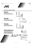
Use the Create Fishnet tool to create a 2 km by 2km polygon grid which cover the C2C
catchments and is based on the locations and spacing of the agcensus data points (See
Figure 6.1).
Figure 6.1: Completed Create Fishnet Form


Use Select by Location... to select the fishnet cells that intersect with (lie on top of) the
C2C model catchments (Figure 6.2).
Export the selection of fishnet cells
o Right-click the fishnet layer in the ArcMap ToC, go to Data>Export Data…. Export
selected features as a new shapefile.
44
Figure 6.2: Selected Fishnet Cells Intersecting the C2C Model Catchments. Red Points
Indicate the Provided agcensus Data Locations.


Modify the coordinates of the agcensus subset data (create new fields either in ArcGIS or
Excel) and calculate the coordinates so that they are equal to the original X or Y
coordinate values + 100. This is so the points fall inside the fishnet cells as opposed to
lying on the SW corner.
Create a new point layer for the agcensus subset data based on these modified
coordinates.
45

Perform a Spatial Join of the modified coordinate agcensus subset data to the C2C
fishnet cells. This links the agcensus data to the relevant fishnet cell.
o Right-click the C2C fishnet layer in the ToC, select Joins and Relates>Joins…. Fill
out the form as shown in figure 6.3
Figure 6.3: Completed Join Data Form



Use the Union tool to combine the spatially joined fishnet output with the C2C model
sub-catchment areas. It is possible to do this for all model sub-catchments at once to
save time. The C2C model sub-catchments data should have fields detailing HSPF
catchment number and sub-catchment number.
o Search for and open the Union tool, add the spatially joined fishnets and the
model sub-catchments as Input Features and assign an Output Feature class.
Open the attribute table for the new Union output layer. Select (using Select by
Attributes…) any rows which are not within a sub-catchment (FID of sub-catchment field
in Union layer = -1).
Delete selected rows (Delete Rows tool)
46



Add a new field to the Union layer, called Area, of type double.
Right-click the new Area field heading, select Calculate Geometry… and calculate the
Area for the field (a metric unit can be used here – this is to be allow calculation of
proportional area).
Export the table of the union layer for use in Excel
o Click the Table Options button in the (attribute) Table window and select
Export....Save the table as a Text File.
The remainder of the calculations can be performed in Excel.







Open the exported table in Excel, selecting commas as the delimiter.
Add a new column called Proportion
Calculate values for the Proportion column as the Area value divided by the area of a full 2
km by 2 km fishnet cell. (match the units used to calculate Area in ArcMap – for example
if using square metres the total fishnet area would be 4000000 m2)
Create new columns for each of the animal counts, call them Prop_[animal] (where
[animal] is the relevant animal name for the field).
Calculate values for each of these new animal fields by multiplying the original count by
the Proportion value. This gives a proportional count of animals based on the area of each
feature row.
If calculations are being undertaken for all catchments (and their sub-catchments) at
once, add another new field called ID.
o Use the concatenate formula to create a unique ID based on the model
catchment and sub-catchment numbers. Use additional letters to distinguish
between the catchment and sub-catchment values so that, for example,
catchment 1, sub-catchment 11 is distinct from catchment 11, sub-catchment 1.
o An example formula would be =CONCATENATE("C",[catchment value
cell],"SC",[sub-catchment value cell])
Copy the Catchment, sub-catchment and ID fields and paste (as values) into a new area
of the worksheet.
o Select all cells in these three columns (including headers) and choose Advanced
from the Sort & Filter section of the Data tab.
o In the Advanced Filter form enter the details as shown in figure 6.4.
o Click OK
Figure 6.4: Completed Excel Advanced Filter Form
47





Use the filtered list of unique combinations of catchments, sub-catchments and IDs as a
new table.
Add columns to the new table for each of the animal types.
o The animal column order should match that of the Animal worksheet in the BIT
spreadsheet to assist with data entry.
Calculate summed proportional numbers for each animal type based on the unique ID
code, rounded to the nearest whole number.
o An example formula would be:
=ROUND(SUMIF($W$2:$W$2255,$AG2,X$2:X$2255),0) where:
 the range $W$2:$W$2255 = range of all ID codes (or sub-catchments
numbers if processing models individually)
 $AG2 = the unique ID code (or sub-catchments number if processing
models individually)
 X$2:X$2255 = the range of proportional animal numbers.
Copy the calculated data and overwrite it by pasting (as values) in the same location. This
is to stop the spreadsheet recalculating the formula.
If all model catchments have been calculated together, use filters to filter according to
model catchment. This allows for the animal count data to be copied into the Animal
worksheet of the relevant catchment BIT spreadsheet.
6.1.4 Manure Application Practices
Manure applications are entered as describe in the BIT documentation and following the
instructions including in the Manure Application worksheet. For each different type of
manure applications are based on the proportion that is applied in each month over a year
and also the proportion that is assumed to be incorporated into the soil.
Advice was taken as to the manure application practices used within the catchments for this
purpose. Consideration has to be taken that, depending on the type of manure, these values
are representative of and applied to all sub-catchments which contain cropland or
pastureland. As a result the monthly proportions will be slightly smoothed under the
assumption that, while practice trends are observed in general, there will be an element of
temporal variation in actual manure application.
6.1.5 Conversion of accumulation values
The HSPF model has a restrictive character length limit for the input values of accumulation
(MON-ACCUM) values and limiting storage (MON-SQOLIM) from the BIT spreadsheet into
HSPF. Values produced by the BIT spreadsheets for the C2C model catchments have subcatchments which exceed this length, especially for the limiting storage values. This resolved
in inaccurate results as the excess character length was excluded leaving much lower values
or even a failure of the model to run if the limiting storage values were falsely recorded as
being lower than the equivalent accumulation values. After consultation with the U.S. EPA
BASINS community (see section 9.5) a workaround was employed to resolve this issue.
The workaround entails that accumulation (MON-ACCUM) and limiting storage (MONSQOLIM) values are divided by 106 to ensure that their input length does not exceed the
characters length restriction in the HSPF code. Additional worksheets have been added to
the BIT spreadsheets (the worksheets are called MON-ACCUM and MON-SQOLIM) which
48
perform this conversion and also correctly format the MON-ACCUM and MON-SQOLIM
values for easier entry into the WinHSPF (see section 7.4).
Once the model has been run any FIO output must be multiplied by 106 to restore the original
values. In practice, the model output data has been multiplied by 105 as HSPF outputs FIO
(Faecal Coliform) water quality components as cfu/litre instead of the more widely used
cfu/100ml. If this step is not performed model data will be several orders of magnitude out
from any observed data.
A final additional worksheet which has been added to the original BIT spreadsheet is Monthly
HSPF input & check. This worksheet was used in the investigation of why the model was not
working before the character length restriction issue was found. It checks that the MONSQOLIM are greater than the MON-ACCUM values. It is redundant in use now, but left for
reference.
6.2 Point Sources
Point source information for urban areas is provided by Will Shepherd in WP1 using the
InfoWorks model. The data from the InfoWorks models are combined according to the
model catchment and sub-catchment into which they drain. A sub-catchment may have more
than one InfoWorks model outflow but these are summed together as the sub-catchment is
essentially the smallest spatial unit which can be used for point source entry.
The InfoWorks model provide separate urban contributions for E.Coli and Confirmed
Enterococci. E.Coli contributions have been used initially as point sources in the HSPF model
runs. The HSPF model is only capable of outputting a single FIO during a model run. In order
to run the model to simulate Confirmed Enterococci, all catchment models would need to be
run again with Confirmed Enterococci point sources used instead of the E.Coli ones.
The InfoWorks outputs are provided per sub-catchment as a time-series output and saved as
a .csv text file in an identical format to that used when preparing the precipitation and
potential evapotranspiration data (sections 3.3.1 and 3.3.2). Although the InfoWorks models
are capable of outputting at a shorter time-step, hourly time-steps are provided to match
the HSPF model time-step. The units of the InfoWorks FIO data are also converted to match
those of the rural FIO inputs which are amended as a result of a model restriction
workaround (see section 6.1.5).
Due to practical consideration of InfoWorks model runtime the InfoWorks models are only
run for 2012. The time-series is modified and extended so that it runs from 00:00 01/01/1998
– 23:00 31/12/2012. Data values prior to 00:00 01/01/2012 are substituted with the average
value during the 2012 model run.
6.2.1 Add to Point Source to .wsd
In order for HSPF to use the InfoWorks time-series data as point sources the relevant .csv
files need to be imported into the catchment model project .wdm that was assigned when
the model was created (section 5.1). The .wdm file can be opened by the WDMUtil file to
allow for the import of the .csv files. The overall process is similar to that detailed in section
3.5.1 when importing .csv files for met data into a met .wdm file. The process for adding the
point source data is listed here.
49








Open WDMUtil
Open the relevant HSPF catchment model project .wdm file (File>Open)
Select File>Import
Locate a saved point source time-series .csv file
Optionally create a template for input or select a previously created template (this can
save time) or select Blank Script and Click Edit
Uncheck the Skip option under Header
Check Character: under Column Format and check that a , [comma] is entered
Check that the data is displayed correctly in the preview – similar to figure 6.5.
Figure 6.5: WDMUtil – Import Script Creation
Figure 6.6: WDMUtil – Import Script Creation – Data Mapping
50





Click the Data Mapping Tab
Enter the values in the input column as shown in figure 6.6.
Click Read Data
Double-click on new time series entry to open the Edit Time Series Attributes window
and allow editing of the attributes.
Add the attributes in table 6.1 according to the dataset and data type you are importing:
Attribute
Scenario
Location
Constituent
Description
Point Source Data
PT-OBS
RCHx (Where x = sub-catchment number)
F.COLIFORM
Hourly
Table 6.1: WDMUtil – Time Series Attributes Entry

An example of a completed Edit Time Series Attribute window for precipitation data is
shown in figure 6.7.
Figure 6.7: WDMUtil – Time Series Attributes


Click OK
Click the Write Time Series to WDM button (outlined in red in figure 6.8)
Figure 6.8: WDMUtil – Write Time Series Tool
o


In the Write to WDM dialogue assign an Output DSN value based on the next
available number from the stored time series.
Repeat the import process for all point source .csv files that represent sub-catchments in
the opened .wsd HSPF catchment model project file.
Repeat for the .wdm project files of all HSPF catchment models.
51
7. Create HSPF Model (Part 2 – FIO)

If not already open, open WinHSPF and load the saved HSPF model (File>Open)
7.1 Add Pollutant



Click the Pollutant Selection button
In the Pollutant Selection window, select F.COLIFORM from the Available pollutants list and click
Add ->.
The Pollutant Selection window should look the same as figure 7.1.
Figure 7.1: WinHSPF – Pollutant Selection

Click OK.
7.2 Edit Control Cards




Click the Control Cards button
In the Control Window Selection window that opens select Descriptions.
In the Control Cards window select the Reaches/Reservoirs tab.
Uncheck HTRCH (this requires additional temperature data) (figure 7.2).
52
Figure 7.2: WinHSPF – Control Cards



Click OK.
Two Control Card Query windows will open, prompting that additional tables are
required as a result of the changes that have been made and asking if you would like to
add them automatically.
Click OK for each window.
7.3 Edit Properties and Enter Accumulations from the BIT


Click the Input Data Editor button
In the Input Data Editor window that opens, navigate to PERLAND>PQUAL
o Double-click QUAL-PROPS
o In the Edit PERLND:QUAL-PROPS window enter 0 in first row of the QIFWFG
column (you may need to scroll right or expand the window to see the column).
o With the text cursor still in the first row cell, double-click the column header to
copy the 0 value down in all rows of that column.
o Repeat this process entering 0 values for columns VIQCFG, QAGWFG and
VAQCFG.
o The finished Edit PERLND:QUAL-PROPS window should look similar to figure 7.3.
53
Figure 7.3: WinHSPF - Finished Edit PERLND:QUAL-PROPS Window

Click OK.

In the Input Data Editor window, return to the first tree level and navigate to
IMPLND>IQUAL
o Double-click on QUAL-INPUT
o In the Edit IMPLND:QUAL-INPUT window enter 0.001 in first row of the SQO
column
o With the text cursor still in the first row cell, double-click the column header to
copy the 0.001 value down in all rows of that column.
o Repeat this process entering the values from table 7.1 for columns POTFW,
ACQOP and SQOLIM.
Parameter
SQO
POTFW
ACQOP
SQOLIM
Value
0.001
0
0
0.00001
Table 7.1: WinHSPF Input Data
o
The finished Edit IMPLND:QUAL-INPUT window should look similar to figure 7.4.
54
Figure 7.4: WinHSPF - Finished Edit IMPLND:QUAL-INPUT Window

Click OK.
7.4 Add Monthly Accumulation Rates and Limiting Storage
Values from BIT
This section makes the final preparations to format data in the BIT spreadsheet for input into
the HSPF model. This requires some entry of values from the HSPF model into the modified
BIT spreadsheets and then formatting and ordering of the BIT accumulation and limiting
storage values before they are then copied into WinHSPF’s input data editor.


If it is not already open, click the Input Data Editor button
In the Input Data Editor window, navigate to PERLAND>PQUAL from the first tree level
o Double-click on MON-ACCUM
o Open the relevant prepared BIT spreadsheet (this must have a matching number
of sub-catchments as well as having been setup as described in section 6.1).
o Switch to the MON-ACCUM worksheet in the BIT spreadsheet.
o Yellow highlighted cells indicate where user input to the worksheet is required.
o In column A of the BIT spreadsheet the Land use numbers for the specific model
need to be entered. These can be found by inspecting the OpNum and Description
columns in the Edit PERLND:MON-ACCUM window. The land use number
corresponds to the final number (the furthest right character) in the OpNum.
Table 7.2 shows an example of this process and figure 7.5 compares the MONACCUM OpNum and Description columns to the equivalent entry in the BIT
spreadsheet.
55
OpNum
(HSPF)
11
16
Description
(HSPF)
Mountain, heath, bog
Water
HSPF Landuse No.
(BIT)
1
6
Table 7.2: Identification of HSPF Land Use Number from OpNum.
Figure 7.5: OpNum and Land Use description in WinHSPF - Edit PERLND:MON-ACCUM
Window Compared with Equivalent HSPF Landuse No. in the MON-ACCUM worksheet of
the BIT Spreadsheet.
o
o
o
Note: OpNum values may change between models or if recreating a model so this
step needs to be checked and/or repeated each time. It is also important to
ensure all land use categories within the model are accounted for. In the example
above the model does not have any “Coast, sea” land use in any of the subcatchments. In other cases you may have to scroll down in the Edit PERLND:MONACCUM window to find all land uses present
In the Bit Tool spreadsheet, on the MON-ACCUM worksheet scroll right until you
find the yellow highlighted Conversion cell (cell V2).
This value should be defaulted to 1000000 (106).
Reason: There is a coded length limit in the input of accumulation (MON-ACCUM)
values into HSPF. For this reason the values are divided by 106 to ensure their input
length does not exceed the number of characters and a lower value is erroneously
stored.
o
o
o
o
o
o
o
In the Edit PERLND:MON-ACCUM window select all of the OpNum values by
clicking in the first cell and dragging down.
Copy the selection by pressing Ctrl+C
In the Bit Tool spreadsheet, on the MON-ACCUM worksheet scroll right until you
find the yellow highlighted OpNum column (column AN)
Click in the first cell below the header (cell AN2) and paste the copied OpNum
values.
The monthly accumulation data is now ordered according to the pasted OpNum
list.
Select the Monthly Accumulation values which have a corresponding OpNum
(entries beyond the list of pasted OpNum should be ignored so you cannot simply
copy the entire columns).
Copy the selected values from the BIT spreadsheet.
56
o
o
o
o
In the Edit PERLND:MON-ACCUM window in WinHSPF, click in the first cell for
QUAJAN at the top of the data input table. Take care not to re-order the table by
clicking on the column headers.
Right-click and select Paste or press Ctrl+V to paste the MON-ACCUM values
from the BIT spreadsheet into the Edit PERLND:MON-ACCUM window.
Visually check that values have copied across correctly for the full range of
OpNum values and months (you will need to scroll the input table to check this).
Your completed table in the Edit PERLND:MON-ACCUM window should look
similar to figure 7.6.
Figure 7.6: WinHSPF – Completed table in the Edit PERLND:MON-ACCUM Window

Click OK.

In the Input Data Editor window, navigate to PERLAND>PQUAL from the first tree level
o Double-click on MON-SQOLIM
o Open the relevant prepared BIT spreadsheet (this must have a matching number
of sub-catchments as well as having been setup as described in section 6.1).
o Switch to the MON-SQOLIM worksheet in the BIT spreadsheet.
o As with the MON-ACCUM worksheet, yellow highlighted cells indicate where user
input to the worksheet is required.
o In column A of the BIT spreadsheet the Land use numbers for the specific model
need to be entered. These can be found by inspecting the OpNum and Description
columns in the Edit PERLND:MON-SQOLIM window (Figure 7.7). The land use
number corresponds to the final number (the furthest right character) in the
OpNum.
o Note: The Land use numbers will be the same as those used for MON-ACCUM for
the same model, so these can be reused.
57
Figure 7.7: OpNum and Land Use description in WinHSPF - Edit PERLND:SQOLIM
Window Compared with Equivalent HSPF Landuse No. in the MON-SQOLIM worksheet of
the BIT Spreadsheet.
o
o
o
Note: OpNum values will be the same for in the MON-ACCUM and MON-SQOLIM
data input tables of the same model but may change between models or if
recreating a model. It is also important to ensure all land use categories within the
model are accounted for. In the example above the model does not have any
“Coast, sea land” use in any of the sub-catchments. In other cases you may have
to scroll down in the Edit PERLND:MON-SQOLIM window to find all land uses
present
In the Bit Tool spreadsheet, on the MON-SQOLIM worksheet scroll right until you
find the yellow highlighted Conversion cell (cell V2).
This value should be defaulted to 1000000 (106).
Reason: There is a coded length limit in the input of limiting storage (MON-SQOLIM)
values into HSPF. For this reason the values are divided by 106 to ensure their input
length does not exceed the number of characters and a lower value is erroneously
stored.
o
o
o
o
o
o
o
o
o
o
o
In the Edit PERLND:MON-SQOLIM window select all of the OpNum values by
clicking in the first cell and dragging down.
Copy the selection by pressing Ctrl+C
Note: OpNum values will be the same as those used for MON-ACCUM for the
same model, so these can be reused.
In the Bit Tool spreadsheet, on the MON-SQOLIM worksheet scroll right until you
find the yellow highlighted OpNum column (column AN)
Click in the first cell below the header (cell AN2) and paste the copied OpNum
values.
The limiting storage data is now ordered according to the pasted OpNum list.
Select the limiting storage values which have a corresponding OpNum (entries
beyond the list of pasted OpNum should be ignored so you cannot simply copy
the entire columns).
Copy the selected values from the BIT spreadsheet.
In the Edit PERLND:MON-SQOLIM window in WinHSPF, click in the first cell for
QUAJAN at the top of the data input table. Take care not to re-order the table by
clicking on the column headers.
Right-click and select Paste or press Ctrl+V to paste the MON-SQOLIM values
from the BIT spreadsheet into the Edit PERLND:MON-SQOLIM window.
Visually check that values have copied across correctly for the full range of
OpNum values and months (you will need to scroll the input table to check this).
58
o
Your completed table in the Edit PERLND:MON-SQOLIM window should look
similar to figure 7.8.
Figure 7.8: WinHSPF - Completed Table in the Edit PERLND:MON-SQOLIM Window

Click OK.

On the Input Data Editor window, Click Close
7.5 Add Point Sources
The point source FIO time-series data can now be added and activated in the model. The
data can be easily added to or removed from the model, which is useful for source
apportionment model runs.











In WinHSPF, with a model open, click the Point Sources button.
In the Point Source window that opens, select the HOURLY (OBS) entry in the Available
point sources list.
Click Add ->
Select HOURLY (OBS) which is now in the In Use point sources list
Check Show Details
Double-click the In Use value in the first row and set the value to Yes in the drop down
menu.
Double-click the In Use field header to copy down the Yes value to all model reaches.
Double-click the Target Member value in the first row and set the value to IDQAL(1) |
dissolved F.COLIFORM in the drop down menu.
Double-click the Target Member field header to copy down the set value to all model
reaches.
The completed Point Sources form should look similar to Figure 7.9.
Click OK.
59
Figure 7.9: Completed Point Sources Window
7.6 Add Model Water Quality (Faecal Coliform) Output









Click the Output Manager button
Select the Output Type as Other.
Click Add.
An Add Output window opens.
In the Operation list select RCHRES X (X), where X is the furthest downstream or exit
sub-catchment. This will be the same number as the flow output you have already added.
In the Group/Member list select GQUAL:DQUAL(1,1)
Check Hourly.
Other values can remain at their defaults.
The Add Output window will appear similar to figure 7.10.
60
Figure 7.10: WinHSPF – Add Output


Click OK.
The Output Manager window will look similar to figure 7.11.
Figure 7.11: WinHSPF – Output Manager

Click Close.
61
The model can now be run to generate hourly concentrations of faecal coliform for the
modelled catchment. At this point you can attempt further calibration of the Water Quality
HSPF model and generate further outputs. Further information on how to do this is available
in later sections.


Click the Run HSPF button
WinHSPF asks if you wish to save new changes to the model (see Figure 7.12).
Figure 7.12: WinHSPF – Save New Changes & Run


Click Save/Run to save and run the model.
You can also save the model without running it by going to File>Save or File>Save As.
62
8. Running the Model

If not already open, open WinHSPF and load a saved HSPF model (File>Open)


Click the Run HSPF button
WinHSPF asks if you wish to save new changes to the model (see below):
Figure 8.1: WinHSPF – Run HSPF

Click Save/Run to save and run the model.
63
9. Common Model Errors
The section is intended to indicate some of the common model errors and issues that have
been experienced when running the HSPF model. The HSPF model provides error reporting
which does offer useful suggestions as to the faults, particularly in identifying the reach of
model segment which is problematic. Other common errors are listed below.
9.1 Issues with input Met data
This can be as a result of erroneous, missing or incorrectly formatted data. Unusually high
precipitation events can indicate an issue with the rain gauge station equipment, if errors
such as this are left unchecked they can percolate through the rest of the model. It is
important to check unusual outputs and link compare them back to the met data (especially
precipitation), this may reveal a previously unidentified issue.
9.2 Data conversion
An issue with both Met data and model output data is that of conversion. It is important to be
vigilant with the conversion of met data from metric to imperial for model processing and
again when converting model output data from imperial to metric. Observed flow data that is
used for calibration will also need to be prepared so that the data matches the same timestep as the model output to ensure a fair comparison. The FIO model output is complicated
by having to be divided by 106 as a workaround to a value character length limit in the model.
This units must be restored by multiplying the output value by 105 (see section 6.1.5).
9.3 FTABLES
FTABLES are Hydraulic Function Tables are used to represent the geometric and hydraulic
properties or each model reach. The values are stored in the .uci file and are generated
when creating the model based on the values stored in the HSPF input files. One of the
properties is linked with the reach length, this can lead to issues with small sub-catchments
with short reach lengths. Because of the small size of the model sub-catchment the
generated FTABLES may not accurately represent the nature of the channel at that point.
This can lead to errors where the volume of water attempting to flow through that reach
exceeds capacity and causes the model calculations to break. The HSPF reporting will
identify which reach the fault has occurred on and the FTABLE that needs attention.
FTABLES can be created both manually and automatically from channel geometries that are
representative of the reach in each sub-catchment. It is possible to edit any problem
FTABLES with real values and using the tools and steps described in BASINS Technical Notes
#1 and #2 (see Appendix H).
Literature has indicated that model accuracy is not dependent on the accuracy of FTABLES
and as a result it is practical to use a common set of FTABLE values when troubleshooting the
model. To do this you should identify the FTABLE reach which has caused the problems from
the HSPF error messages. Then find the FTABLE entry for that reach in the HSPF .uci file see
figure 9.1 for an example). A problematic FTABLE will have a small range of depth values and
generally low values throughout the FTABLE. Select another FTABLE from the same .uci file if
practical (or another working model .uci file if not) and copy the FTABLE to replace the
64
problematic one. Save changes to the .uci file and attempt to run the model again.
Remember to save a copy of the original .uci file when making manual edits.
FTABLE
1
rows cols
8
4
depth
area
0.
1.69
0.5
1.78
5.
2.54
6.25
2.75
7.81
8.36
9.38
8.88
160.94
60.19
312.5
111.49
END FTABLE 1
***
volume outflow1 ***
0.
0.
0.87
20.89
10.58
988.9
13.88
1456.99
26.53
2169.22
40.
4119.32
5274.223820278.75
18283.63 20067014.
Figure 9.1: Example FTABLE in a .uci File
9.4 Errors when using BASINS to delineate sub-catchments
BASINS can struggle with delineation of small model catchments and low relief topography. It
also is less intuitive to process single sub-catchment model outputs. If the BASINS delineated
sub-catchments do not match the full model extent or fail to generate entirely the subcatchment delineation should be attempted using the Arc Hydro Tools method (section
3.2.2).
9.5 Getting additional help
The U.S. EPA run an online community which is very helpful in solving problems with BASINS
and HSPF. The community operates as a Listserv, details for joining the BASINS Listserv are
included
below
and
are
taken
from
the
Contact
Information
at
http://water.epa.gov/scitech/datait/models/basins/index.cfm
BASINS Listserv: Join this online community of BASINS users to exchange questions
and answers regarding the use of BASINS.
Join the BASINS listserv by sending an email to [email protected], leaving the
"Subject:" field blank and putting "subscribe basinsinfo firstname lastname" in the
body of the text. Once you have subscribed, you will receive a welcome message
confirming your membership.
Search the BASINS listserv archives (as well as other EPA forums to which you are
subscribed) by going to https://lists.epa.gov/read/. Login, then go to “My
Forums”. Select the forum you want (e.g., basinsinfo). Then click on
“Search”. There is also a link for Advanced Search.
You can also contact EPA's BASINS Support Team to find additional information on
BASINS not answered through the BASINS Listserv.
From: http://water.epa.gov/scitech/datait/models/basins/index.cfm
65
10. Outputting Model Results
Once a model Run has completed the model outputs can be viewed and plotting using the
GenScn program that is provided with WinHSPF and BASINS. The GenScn software also
allows the data to be exported so that it can be used in spreadsheet and other software for
further analysis.
10.1 Viewing Model Results

For a model that has just been run, or has been run previously and saved, click the View

Output through GenScn button in WinHSPF.
The GenScn window opens and provides lists of model Locations, Scenarios and
Constituents (Figure 10.1).
In the Constituents list select DQAL1 and FLOW so they are highlighted in grey.


In the Time Series section click the add to Time-series List button
Time series data of the FLOW and DQAL1 constituents are added to the list

Figure 10.1: GenScn Window

You can double click the data to view the attributes of each time series. This is useful to
identify which is the hourly flow time series (typically DSN 1001) from the daily flow data
(typically DSN 101).
66


Click on the hourly FLOW data in the Time Series list to highlight it grey.
In the Dates section under Current enter the date range 2012/1/1 – 2012/12/30 (in
YYYY/MM/DD format) as shown in figure 10.1.
Reason: 2012 was selected as the year in which to run both rural and urban models and
provide input to the river and estuary model. The end date of 30th December 2012 marks the
end date of the currently provided MORECS potential evapotranspiration data. And as a
result determines the end date of the 2012 model output.



To view the data in a plot, click the Generate Graphs button
In the Graph window that is opened click Generate.
A plot of the selected flow data for the entered data range is produced (similar to figure
10.2)
Figure 10.2: Example GenScn Plot



The plot type, style and format can be adjusted with the settings found under the Edit
menu in the Genscn Standard Plot window.
Plots can be copied to the clipboard or saved as image files by going to File>Save
Once finished close the Genscn Standard Plot and Graph windows.
10.2 Exporting Model Output Data

Returning to the GenScn window and ensure the FLOW and DQAL1 constituents are still
added to the Time Series list and the Current date range in the Dates section is entered
as 2012/1/1 – 2012/12/30 (as described in section 10.1).
67

In the Time Series section, select both the hourly FLOW (likely to be DSN 1001, this can be
confirmed by double-clicking the time series entry and inspecting the attributes) and the
DQAL1 time series entries. Hold down Ctrl when selecting multiple entries.


Click the List Timeseries Values button in the Analysis section
In the Timeseries Data window which opens go to Edit>Number Format to be able to edit
the number format of the model outputs.
Using the value as shown in table 10.1, click in the corresponding cells in the Timeseries
Data window table, pressing return to ensure the changes are applied.

Number Format
FLOW
DQAL1
Number Width
10
10
Significant Digits
10
10
Decimal Places
5
8
Table 10.1 Number Format Values for Model Outputs

The completed and correctly formatted output table should look similar to the one
shown in figure 10.3.
Figure 10.3: Timeseries Data Window with Number Format Options Completed





To export the data table go to File>Save to Text File
Check Character delimited: and ensure a , [comma] is entered in the character text box
Navigate to and select the location to save the output text file.
Enter an appropriate filename and include a .csv file extension.
The completed dialog window should look similar to figure 10.4.
68
Figure 10.4: Save To Text File Dialog


Click OK
The exported .csv file can be opened in MS Excel and other comparable software. The file
will contain both flow data (in ft3s-1) and FIO data (in (cfu/litre) x 10-6) which can be
converted back to metric data, analysed further and used to plot outputs accordingly. In
the case of the FIO data multiplying the model output by 105 will convert it to correct
values in the more commonly used cfu/100ml units.
69
11. Calibration
A brief overview of some of the considerations to HSPF model calibration is given in this
section. Additional sources (links to which are provided in Appendix H) are also suggested
which give much further detail and guidance. A reminder on ensuring the model outputs are
converted into appropriate units is also included.
11.1 Hydrological Calibration
Hydrological calibration is performed by comparing the model output data against observed
flow data at the same locations in the catchment if the data is available. Calibration methods
can target overall agreement, agreement at high or low flow and response to specific storm
events. This calibration targets may be determined by the purpose of the model or where
the model results appear weakest. Checks can be made visually to the hydrograph of the
modelled flow plotted against the observed flow. Statistical analysis should also be made to
the two sets of data. Visual checks and checks against volumes should be made at annual,
seasonal, month and storm event time periods. Detailed information on the calibration
process is provided by the BASINS Tutorials and Training documentation, in particular
Exercise 6 - WinHSPF Hydrology Calibration and Lecture 15 - Watershed Model Calibration
and Validation. Links to these are provided in Appendix H.
Changes made to the model parameters can have different influences on the model outputs.
Some may raise the base level flow, while others can storm response and affect peak flows.
The manual process is iterative with each change made to a parameter having the new
output analysed to assess the difference it makes. Descriptions of the different hydrological
parameters are provided in Technical Note #6 - Estimating Hydrology and Hydraulic
Parameters for HSPF. Advice of which parameters to change based on the differences
between observed and modelled data is provided in Appendix A of the HSPEXP
documentation. Links to both documents are provided in Appendix H
11.1.1 Interactive and Automated Hydrological Calibration
A (semi-) automated calibration process is also possible with additional programmes and
utilities such as HSPEXP and PEST. HSPEXP is provides an interactive process to compare
plots and statistics of observed values against simulated ones, it also provides expert advice
on which parameters should be changed to improve calibration. Additional exercises and
material regarding HSPEXP are provided in Appendix H (See Exercise 7 and Appendix D in
the BASINS Tutorials and Training and the HSPEXP section). PEST is a software package that
provides model-independent parameter estimation and uncertainty analysis. It is compatible
with a modified version of the HSPF model (such as the one used here) and can automate
the calibration process. Further information is available for the links provided under the
PEST section in Appendix H.
11.1.2 Flow Data Conversion
The HSPF model runs, by default, in imperial units. It was decided that that should be
maintained to avoid unforeseen conversion issues. Input data was converted into the
70
relevant imperial units. The output modelled data should be converted back to metric units
for calibration.

Conversion to ft3s-1 from m3s-1.
o
Multiply m3s-1 values by 35.3146667 to get ft3s-1.
11.2 FIO calibration
Calibration of FIO data is more difficult that calibrating the hydrological element of the model
as observed FIO data is not available in a continuous time-series. For this reason it is
important to concentrate on the overlap of model and observed data and also to select key
points in the sampling period.
Making calibration adjustments to the FIO outputs can be made either through modifications
to the Bacteria Indicator Tool (BIT) spreadsheets, which results in changes to the FIO
accumulations, or by changing the parameter that controls the decay rate of the FIO
constituent being modelled in HSPF.
11.2.1 BIT calibration
Changes to the BIT spreadsheets can be made in any of the worksheets (see section 6.1).
Each change would have a knock-on effect to the final FIO accumulations. It may also be
advisable to make changes to the reference values on the References worksheet. These
values are based on literature and are used in all calculations of accumulation rates.
Changing these values will have an overall impact without having to alter livestock counts and
sub-catchment land use areas. The reference values can be replaced by more accurate
locally measured values or simply calibrated based on the modelled FIO output.
11.2.2 FIO Decay rate
Changes to the decay rate of FIO will also have an influence on the FIO model outputs. The
decay rate parameter can be accessed using the Input Data Editor following the steps
outlined below (see also section 7.3).



Click the Input Data Editor button
In the Input Data Editor window that opens, navigate to RCHRES>GQUAL
o Double-click GQ-GENDECAY
o The FSTDEC column stores the first order decay rate for the FIO constituent.
o You can make edits to the FSTDEC values directly to the cells in the GQGENDECAY table.
o The OpNum values in the GQ-GENDECAY table refer to the model sub-catchment
numbers.
o You can copy a value entered in the first cell of the FSTDEC column down to all
cells in the column by double-clicking the column header (with the text cursor
still in the first row cell).
o The finished Edit PERLND:QUAL-PROPS window should look similar to figure 11.1.
o Click OK to save changes
Save or Save and Run the model before exiting WinHSPF.
71
Figure 11.1: WinHSPF – Edit RCHRES:GQ-GENDECAY Window
11.2.3 FIO Data Conversion
The HSPF model runs, by default, in imperial units. It was decided that that should be
maintained to avoid unforeseen conversion issues. For FIO data model input values also have
to be modified for a workaround to overcome a character length restriction in their data
entry. The model output values must be converted back to be able to compare them against
observed data.

Conversion to cfu/100ml from (cfu/litre) x 106.
o
Multiply (cfu/litre) x 106 values by 105 to get cfu/100ml.
72
12. Model Changes for Scenario Modelling
This provides some suggestions as to how scenario modelling could be implemented using
the HPSF model, which input files would require changing and how the original model would
be affected. Considerations have been made for both future management and climate
scenarios.
12.1 Management Scenarios
Management scenario changes could be reflected in the HSPF model be modifications to the
BIT spreadsheet FIO accumulation values, changes to the urban point source FIO
contributions and amending the land use areas or configuration within the model subcatchments.
12.1.1 BIT spreadsheet changes
Exploring possible future management scenarios with HSPF will likely be achieved by making
changes to the BIT spreadsheet and the resulting FIO accumulation values. Changes could be
made to individual worksheets. This may be as changes to animal numbers, changes to
manure application (in terms of trends, amount and associated FIO concentrations), changes
to grazing practices and changes to the access to streams for cattle. This method would
allow for direct and tangible ‘real world’ changes to be explored. Information on the BIT
spreadsheet can be found in section 6.1.
An alternate would be to apply a proportional reduction or increase to the final MONACCUM values for each land use and sub-catchment. A change to the MON-ACCUM values
should also be reflected in the MON-SQOLIM values. A simple method to achieve a change
would be to amend the conversion value found in the BIT spreadsheet MON-ACCUM and
MON-SQOLIM worksheets (see section 7.4). This value is used to reduce the size of the
accumulation values but in theory could also be used to modify the value as well.
12.1.2 Urban Point Source Changes
Changes to FIO contributions in urban areas would need to be reflected in the point source
files provided by InfoWorks (section 6.2). If the data is modified as a result of new InfoWorks
model runs then new output .csv time series files would need to be created and input into
the HSPF .wdm project file. These could be in place alongside the current condition point
sources time-series and identified using a different range of DSN numbers as well as a
modified description. In WinHSPF the a new set of point sources should be shown in the
available list which could then be added and set to being in use, while the current condition
point sources are removed (see section 7.5). It may be more practical to take of copy of an
existing model and replace the point source time-series data in the copied .wdm file.
If simple, mathematical, modifications are to be performed on the urban point sources this
could be achieved within the WDMUtil software. Steps to achieve this are the same as those
suggested in section 12.2.2 for modifying met data.
73
12.1.3 Land Use Changes
Future changes in land use can also be explored. A redistribution of areas within each model
sub-catchment could be achieved by the following:




Manually amended the area values in the SCHEMATIC section of the .uci file (see
Appendix G)
o Note - the total area of all land use types within the sub-catchment should be
unchanged.
Updating the land use worksheet of the BIT spreadsheet with the redistributed area
values.
Updating the recalculated MON-ACCUM and MON-SQOLIM values from the revised BIT
spreadsheet.
Re-running the model.
The above suggested method is untested but should work in theory. An alternative would be
to modify the .wsd HSPF input file (section 4.2.1 and 4.2.2) and recreate the HSPF model
(section 5).
Changing the .wsd HSPF input file and recreating the model would also allow for changes in
the configuration of the land use within the sub-catchments. While the sub-catchments
themselves should remain unchanged, it would allow for the removal or addition of any
model operations (i.e. the unique combination of land use categories within each subcatchment). For example removing "Arable & horticultural" land use from a sub-catchment
or adding “Grassland” as a new land use within a sub-catchment would be possible.
Attempting to make a change such as that without recreating the model, would likely cause
further complications and break the HSPF model. (It might be possible to set land uses you
wish to delete to 0 in the .uci file, but that is again untested and may remain problematic).
12.2 Climate Scenarios
Future climate change scenarios would be reflected in the HSPF model by modifying the met
data that is input into the model and drives the hydrological component of HSPF. The met
time-series data would either be replaced by newly generated time-series or the existing
time-series data could be modified if simple mathematical changes are acceptable.
12.2.1 Generating New Met Data
The generation of new met data would require the use of an additional resource to provide
the met data. Potential options that have been preliminarily explored are:



Future Flows (CEH)
Weather Generator (DEFRA)
Hyetos
Links for further information on the above are provided in the Climate Change Met Data
Generation section of Appendix H.
74
Any newly generated time-series data for precipitation and/or evapotranspiration would
need preparing and importing into a new .wdm file using the same steps as detailed in
sections 3.3 and 3.5.
A copy of the current model could be taken and the repointed to a new met .wdm file. This
would be achieved by modifying the .uci file and changing the location of the WDM2 file in the
.uci File section (see Appendix G). Hopefully the copied model will open successfully and you
to replace the existing met segments by adding the new ones and reassigning the
connections (see section 5.3). This process is untested, if it fails to work or breaks the model
an alternative would be to recreate the model and use the new met .wdm file when creating
it (as in section 5.1 and 5.2).
12.2.2 Modifying Existing Met Data
Simple mathematical changes can be made to existing met time-series data using the
WDMUtil software. The tool allows for calculations to be made using existing time-series data
or numeric values. Using precipitation as an example, it would be possible to multiply a value
to create a new time-series of proportionally increased or decreased precipitation or
evapotranspiration. It would also be possible to generate an additional time-series of varying
(perhaps by month or season) proportional values and using that to multiply with the existing
precipitation time-series. This method could be used to generate, for example, a time-series
with wetter summers and drier winters based on the existing precipitation time-series data.
The steps to access this functionality in the WDMUtil software are shown below.


Open the WDMUtil software and load an existing met .wdm file (File>Open)
Click the Generate Time Series button in the Tools section (highlighted in red in figure
12.1)
Figure 12.1: WDMUtil - Generate Time Series Button




In the New Time Series window that opens click on the Math tab.
Calculations can be performed on the existing time series on this tab using the provided
mathematical functions or operators and selecting the relevant existing time-series data
or entering numeric values. An example is shown in figure 12.2.
Edit the Description of the New Properties for the output time-series
Leave the Save in option as <in memory>, this gives you the option of saving the output as
a new time-series (with a new DSN value) or overwriting the existing time-series by
saving it with the same DSN value.
o The former option should be used if retaining all met time-series data in the same
met .wdm file.
o The latter option can be used if a copy of the met .wdm file has been taken.
o The steps to save an in memory time-series are described in section 3.5.1.
75
Figure 12.2: WDMUtil – New Time Series Window
With modified met data, the HSPF model can be run once the following changes have been:


If the new climate change time-series data has been saved in the original met .wdm (with
existing observed time-series) then the model met segments will need to be amended see section 5.3
If a new met .wdm has been created then the model .uci file will need modifying by
changing the location of the WDM2 file in the .uci File section (see Appendix G).
o This process is untested, if it fails to work or breaks the model an alternative
would be to recreate the model and use the new met .wdm file when creating it
(as in section 5.1 and 5.2).
76
Appendices
Appendix A – ArcMap Model Builder Diagrams for .ptf and .rch HSPF Input Files
The following ArcMap Model Builder diagrams detail the work flow in creating a shapefile based on the Arc Hydro tools DrainageLine output (see
section 3.2.2). The output contains measured values required in the creation of the .ptf and .psr HSPF model input files. There are three Model Builder
diagrams which should be performed in sequence. The first prepares new fields in the DrainageLine shapefile and calculates HSPF sub-catchment
numbers and values of reach length based on the DrainageLine features and attributes.
77
The second diagram continues processing the DrainageLine shapefile. Here it identifies the exit sub-catchment and then joins a copy of the
DrainageLine shapefile as an intermediary file to translate the Arc Hydro Tools NextDownID field into HSPF sub-catchment numbers.
78
The final diagram, and step in the calculations, uses the DEM and a percent rise slope raster (calculated separately from the DEM) to calculate and add
the final values of average slope along the reach, average elevation along the reach and the difference between the minimum and maximum elevation
along the reach. All values that are required to create the .ptf and .rch HSPF input files are now contained in the processed DrainageLine shapefile.
79
Appendix B – ArcMap Model Builder Diagrams for .wsd HSPF Input File
The following ArcMap Model Builder diagrams detail the work flow in creating a shapefile based on the Arc Hydro tools Catchment output (see section
3.2.2). The output contains measured values required in the creation of the .wsd HSPF model input files. The Model Builder diagrams should be
performed in sequence although first two diagrams are used for processing a model catchment that contains multiple sub-catchments and the third
diagram performs the equivalent steps for a model catchment consisting of a single sub-catchment. The fourth diagram contains the final steps for
both types of model catchment.
The Diagram below should be the initial step for a model catchment with multiple sub-catchments. The model processes the HSPF categorised land
use data for each sub-catchment, allowing the area of each land use category within each sub-catchment to be calculated. The model creates a new
shapefile called WSD to store these areas and also adds additional fields required for the .wsd HSPF input file and assigns HSPF sub-catchment
numbers and appropriate default values. The model also performs the initial calculation of average percent rise slope values per sub-catchment.
80
The model below is the second step for processing model catchments with multiple sub-catchments. The model uses the pre-processing of average
percent rise slope values for the sub-catchments and joins and writes the data to the appropriate field in the WSD shapefile output.
81
The Diagram below is the initial step for a model catchment with a single sub-catchment. The model processes the HSPF categorised land use data for
the sub-catchment, allowing the area of each land use category to be calculated. The model creates a new shapefile called WSD to store these areas
and also adds additional fields required for the .wsd HSPF input file and assigns HSPF sub-catchment numbers and appropriate default values. The
model also records the average percent rise slope of the sub-catchment, which is based on a value calculated outside of this model and entered as a
parameter manually.
82
The final model diagram shows the final stage of processing that should be performed on the WSD shapefiles from models with both single and
multiple sub-catchments. The model details the steps required to duplicate ‘Built-up areas’ so that this HSPF land use category is represented by both
an impervious and pervious entry. The ‘Built-up areas’ are divided equally between the two types, accordingly the areas are halved meaning that the
sum of the pervious and impervious areas of ‘Built-up areas’ equals the total area for the ‘Built-up areas’ in the model sub-catchment or subcatchments.
83
Appendix C – .psr File Example
The .psr file stores Point Sources information. It is a text file saved as XX.psr, where XX is the filename.
Note: all HSPF input files must have the same filename and be stored in the same directory when creating an HSPF model in WinHSPF.
The .psr input file is left as the default, point sources used within the model are added as time series data in the model output .wdm file and
selected and marked in use in WinHSPF.
0
FacilityName Npdes Cuseg Mi
OrdinalNumber Pollutant Load(lbs/hr)
84
Appendix D – .ptf File Example
The .ptf file store Channel Geometry information. It is a text file saved as XX.ptf, where XX is the filename.
Note: all HSPF input files must have the same filename and be stored in the same directory when creating an HSPF model in WinHSPF.
The example file below is for 7 sub-catchments within the model. The header row (stored on one line – it is word wrapped here) is comma
delimited with all header text qualified with speech marks (“). The data entries are space delimited, speech marks are not required for the data
text entry. The data for each sub-catchment is entered on a new row. The number of decimal places varies with column, the formatting was
matched to the outputs produced by BASINS for consistency and compatibility.
"Reach Number","Length(ft)","Mean Depth(ft)","Mean Width (ft)","Mannings Roughness Coeff.","Long. Slope","Type of xsection","Side slope of upper FP left","Side slope of lower FP left","Zero slope FP width left(ft)","Side slope of
channel left","Side slope of channel right","Zero slope FP width right(ft)","Side slope lower FP right","Side slope
upper FP right","Channel Depth(ft)","Flood side slope change at depth","Max. depth","No. of exits","Fraction of flow
through exit 1","Fraction of flow through exit 2","Fraction of flow through exit 3","Fraction of flow through exit
4","Fraction of flow through exit 5"
1 3686 5.00000 30.00000 0.05 0.01249 Trapezoidal 0.5 0.5 30.000 1 1 30.000 0.5 0.5 6.2500 9.3750 312.500 1 1 0 0 0 0
3 4464 5.00000 30.00000 0.05 0.00844 Trapezoidal 0.5 0.5 30.000 1 1 30.000 0.5 0.5 6.2500 9.3750 312.500 1 1 0 0 0 0
2 9755 5.00000 30.00000 0.05 0.02327 Trapezoidal 0.5 0.5 30.000 1 1 30.000 0.5 0.5 6.2500 9.3750 312.500 1 1 0 0 0 0
4 415 5.00000 30.00000 0.05 0.03414 Trapezoidal 0.5 0.5 30.000 1 1 30.000 0.5 0.5 6.2500 9.3750 312.500 1 1 0 0 0 0
5 10024 5.00000 30.00000 0.05 0.03480 Trapezoidal 0.5 0.5 30.000 1 1 30.000 0.5 0.5 6.2500 9.3750 312.500 1 1 0 0 0 0
6 5213 5.00000 30.00000 0.05 0.00905 Trapezoidal 0.5 0.5 30.000 1 1 30.000 0.5 0.5 6.2500 9.3750 312.500 1 1 0 0 0 0
7 10801 5.00000 30.00000 0.05 0.12221 Trapezoidal 0.5 0.5 30.000 1 1 30.000 0.5 0.5 6.2500 9.3750 312.500 1 1 0 0 0 0
85
Appendix E – .rch File Example
The .rch file stores Reach information. It is a text file saved as XX.rch, where XX is the filename.
Note: all HSPF input files must have the same filename and be stored in the same directory when creating an HSPF model in WinHSPF.
The example file below is for 7 sub-catchments within the model. The header row (stored on one line – it is word wrapped here) is comma
delimited with all header text qualified with speech marks (“). The data entries are space delimited, speech marks are required to surround the
entry of data in the Pname column. The data for each sub-catchment is entered on a new row. The number of decimal places varies with column,
the formatting was matched to the outputs produced by BASINS for consistency and compatibility.
"Rivrch","Pname","Watershed-ID","HeadwaterFlag","Exits","Milept","Stream/Resevoir
Type","Segl","Delth","Elev","Ulcsm","Urcsm","Dscsm","Ccsm","Mnflow","Mnvelo","Svtnflow","Svtnvelo","Pslope","Pdepth","
Pwidth","Pmile","Ptemp","Pph","Pk1","Pk2","Pk3","Pmann","Psod","Pbgdo","Pbgnh3","Pbgbod5","Pbgbod","Level","ModelSeg"
1 "1" 1 0 1 0 S 0.70 10.50 41 0 0 4 0 0 0 0 0 0.012494 5.0000 30.000 0 0 0 0 0 0 0 0 0 0 0 0 0 1
3 "3" 3 0 1 0 S 0.85 9.19 46 0 0 4 0 0 0 0 0 0.008445 5.0000 30.000 0 0 0 0 0 0 0 0 0 0 0 0 0 1
2 "2" 2 0 1 0 S 1.85 36.09 52 0 0 5 0 0 0 0 0 0.023272 5.0000 30.000 0 0 0 0 0 0 0 0 0 0 0 0 0 1
4 "4" 4 0 1 0 S 0.08 8.53 38 0 0 5 0 0 0 0 0 0.034140 5.0000 30.000 0 0 0 0 0 0 0 0 0 0 0 0 0 1
5 "5" 5 0 1 0 S 1.90 34.12 28 0 0 8 0 0 0 0 0 0.034800 5.0000 30.000 0 0 0 0 0 0 0 0 0 0 0 0 0 1
6 "6" 6 0 1 0 S 0.99 6.23 13 0 0 8 0 0 0 0 0 0.009055 5.0000 30.000 0 0 0 0 0 0 0 0 0 0 0 0 0 1
7 "7" 7 0 1 0 S 2.05 26.25 10 0 0 -1 0 0 0 0 0 0.122214 5.0000 30.000 0 0 0 0 0 0 0 0 0 0 0 0 0 1
86
Appendix F – .wsd File Example
The .wsd file is the Watershed information. It is a text file saved as XX.wsd, where XX is the filename.
Note: all HSPF input files must have the same filename and be stored in the same directory when creating an HSPF model in WinHSPF.
The example file below is for 7 sub-catchments within the model. Each sub-catchment has a separate entry for each land use type within the subcatchment. Built-up areas are duplicated with an impervious entry and a pervious entry, the combined area of both Built-up area entries for each
sub-catchment equals the total Built-up area within the sub-catchment. The division of impervious and pervious Built-up area used here is equal –
50% allocated to each.
The header is comma delimited with all header text qualified with speech marks (“). The data entries are space delimited (5 spaces are used in this
file), speech marks are required to surround the entry of data in the LU Name column. The data for each land use area and type
(pervious/impervious) within each sub-catchment is entered on a new row. The number of decimal places varies with column, the formatting was
matched to the outputs produced by BASINS for consistency and compatibility.
"LU Name","Type (1=Impervious, 2=Pervious)","Watershd-ID","Area","Slope","Distance"
"Arable & horticultural"
2
1
181.0
0.023937
0.0000
"Arable & horticultural"
2
2
467.1
0.029466
0.0000
"Arable & horticultural"
2
3
268.8
0.032704
0.0000
"Arable & horticultural"
2
5
185.8
0.025124
0.0000
"Arable & horticultural"
2
6
225.9
0.017593
0.0000
"Arable & horticultural"
2
7
255.4
0.016834
0.0000
"Built-up areas"
1
1
5.6
0.023937
0.0000
"Built-up areas"
1
2
281.4
0.029466
0.0000
"Built-up areas"
1
3
11.4
0.032704
0.0000
"Built-up areas"
1
5
86.2
0.025124
0.0000
"Built-up areas"
1
6
65.8
0.017593
0.0000
"Built-up areas"
1
7
64.5
0.016834
0.0000
"Coast, Sea"
2
7
64.4
0.016834
0.0000
"Grassland"
2
1
407.8
0.023937
0.0000
"Grassland"
2
2
541.3
0.029466
0.0000
"Grassland"
2
3
414.1
0.032704
0.0000
"Grassland"
2
4
2.5
0.035626
0.0000
"Grassland"
2
5
851.2
0.025124
0.0000
87
"Grassland"
2
"Grassland"
2
"Mountain, heath,
"Mountain, heath,
"Mountain, heath,
"Water"
2
"Woodland"
2
"Woodland"
2
"Woodland"
2
"Woodland"
2
"Woodland"
2
"Built-up areas"
"Built-up areas"
"Built-up areas"
"Built-up areas"
"Built-up areas"
"Built-up areas"
6
7
bog"
bog"
bog"
7
1
2
3
6
7
2
2
2
2
2
2
790.0
639.1
2
2
2
12.0
0.4
46.5
34.5
38.1
7.6
1
2
3
5
6
7
0.017593
0.0000
0.016834
0.0000
2
5.6
0.029466
0.0000
3
3.6
0.032704
0.0000
6
0.4
0.017593
0.0000
0.016834
0.0000
0.023937
0.0000
0.029466
0.0000
0.032704
0.0000
0.017593
0.0000
0.016834
0.0000
5.6
0.023937
0.0000
281.4
0.029466
0.0000
11.4
0.032704
0.0000
86.2
0.025124
0.0000
65.8
0.017593
0.0000
64.5
0.016834
0.0000
88
Appendix G – .uci File Example
The .uci file is the User Control Input file which contains all parameters and instructions needed to
run the HSPF model. The text file is tightly formatted and arranged in a preordained order which is
readable by the HSPF model software. The file is created by WinHSPF from the model input files
that are either created by BASINS or manually using the Arc Hydro method. Changes to parameters
and model configuration made in WinHSPF will be recorded and stored in the .uci file. It is also
possible (and sometimes simpler) to edit the .uci file directly, making quick parameter adjustments
in a text editor, saving the changes and then reading them into HSPF when the model is next
opened.
The included .uci file example is for a model of 7 sub-catchments.
RUN
GLOBAL
UCI Created by WinHSPF for 12
START
2003/01/01 00:00 END
RUN INTERP OUTPT LEVELS
1
0
RESUME
0 RUN
1
END GLOBAL
2012/12/30 00:00
UNITS
FILES
<FILE>
MESSU
1
<UN#>***<----FILE NAME------------------------------------------------->
24
12.ech
91
12.out
WDM1
25
12.wdm
WDM2
26
..\..\Met\C2C_MET.wdm
BINO
92
12.hbn
END FILES
OPN SEQUENCE
INGRP
PERLND
PERLND
PERLND
PERLND
IMPLND
PERLND
PERLND
PERLND
PERLND
PERLND
IMPLND
PERLND
PERLND
PERLND
PERLND
PERLND
IMPLND
PERLND
PERLND
PERLND
PERLND
IMPLND
PERLND
PERLND
PERLND
INDELT 01:00
101
103
106
107
101
301
303
304
306
307
301
201
203
204
206
207
201
403
501
503
507
501
601
603
604
89
PERLND
PERLND
IMPLND
PERLND
PERLND
PERLND
PERLND
PERLND
PERLND
IMPLND
RCHRES
RCHRES
RCHRES
RCHRES
RCHRES
RCHRES
RCHRES
END INGRP
END OPN SEQUENCE
606
607
601
701
702
703
705
706
707
701
1
3
2
4
5
6
7
PERLND
ACTIVITY
*** <PLS >
Active Sections
***
*** x - x ATMP SNOW PWAT SED PST PWG PQAL MSTL PEST NITR PHOS TRAC ***
101 707
0
0
1
1
0
0
1
0
0
0
0
0
END ACTIVITY
PRINT-INFO
*** < PLS>
*** x - x ATMP SNOW PWAT
101 707
4
4
4
END PRINT-INFO
SED
4
Print-flags
PIVL
PST PWG PQAL MSTL PEST NITR PHOS TRAC
4
4
4
4
4
4
4
4
1
BINARY-INFO
*** < PLS>
Binary Output Flags
PIVL
*** x - x ATMP SNOW PWAT SED PST PWG PQAL MSTL PEST NITR PHOS TRAC
101 707
4
4
4
4
4
4
4
4
4
4
4
4
1
END BINARY-INFO
GEN-INFO
***
Name
*** <PLS >
*** x - x
101
Arable & horticultur
103
Grassland
106
Woodland
107
Built-up areas
201
Arable & horticultur
203
Grassland
204
Mountain, heath, bog
206
Woodland
207
Built-up areas
301
Arable & horticultur
303
Grassland
304
Mountain, heath, bog
306
Woodland
307
Built-up areas
403
Grassland
501
Arable & horticultur
503
Grassland
507
Built-up areas
Unit-systems
Printer BinaryOut
t-series Engl Metr Engl Metr
in out
1
1
0
0
92
0
1
1
0
0
92
0
1
1
0
0
92
0
1
1
0
0
92
0
1
1
0
0
92
0
1
1
0
0
92
0
1
1
0
0
92
0
1
1
0
0
92
0
1
1
0
0
92
0
1
1
0
0
92
0
1
1
0
0
92
0
1
1
0
0
92
0
1
1
0
0
92
0
1
1
0
0
92
0
1
1
0
0
92
0
1
1
0
0
92
0
1
1
0
0
92
0
1
1
0
0
92
0
90
PYR
9
PYR
9
601
Arable & horticultur
603
Grassland
604
Mountain, heath, bog
606
Woodland
607
Built-up areas
701
Arable & horticultur
702
Coast, Sea
703
Grassland
705
Water
706
Woodland
707
Built-up areas
END GEN-INFO
PWAT-PARM1
*** <PLS >
*** x - x CSNO RTOP UZFG
101 707
0
1
1
END PWAT-PARM1
1
1
1
1
1
1
1
1
1
1
1
Flags
VCS VUZ
1
0
1
1
1
1
1
1
1
1
1
1
1
VNN VIFW VIRC
0
0
0
PWAT-PARM2
*** < PLS>
FOREST
*** x - x
101 107
1.
201 207
1.
301 307
1.
403
1.
501 507
1.
601 607
1.
701 703
1.
705
0.
706 707
1.
END PWAT-PARM2
LZSN
(in)
6.5
6.5
6.5
6.5
6.5
6.5
6.5
4.
6.5
INFILT
(in/hr)
0.16
0.16
0.16
0.16
0.16
0.16
0.16
0.16
0.16
LSUR
(ft)
350
350
300
300
350
350
350
350
350
PWAT-PARM3
*** < PLS>
PETMAX
*** x - x
(deg F)
101 707
40.
END PWAT-PARM3
PETMIN
(deg F)
35.
INFEXP
PWAT-PARM4
*** <PLS >
CEPSC
*** x - x
(in)
101 707
0.1
END PWAT-PARM4
UZSN
(in)
1.128
0
0
0
0
0
0
0
0
0
0
0
0
0
0
0
0
0
0
0
0
0
0
VLE IFFC
1
1
0
0
0
0
0
0
0
0
0
0
0
HWT IRRG IFRD
0
0
0
0.023937
0.029466
0.032704
0.035626
0.025124
0.017593
0.016834
0.016834
0.016834
KVARY
(1/in)
0.
0.
0.
0.
0.
0.
0.
0.
0.
AGWRC
(1/day)
0.98
0.98
0.98
0.98
0.98
0.98
0.98
0.98
0.98
INFILD
DEEPFR
BASETP
AGWETP
2.
2.
0.1
0.02
0.
NSUR
INTFW
LZETP
0.2
0.75
IRC
(1/day)
0.5
IFWS
0.01
LZS
1.5
AGWS
0.01
PWAT-STATE1
*** < PLS> PWATER state variables (in)
*** x - x
CEPS
SURS
UZS
101 707
0.01
0.01
0.3
END PWAT-STATE1
SLSUR
92
92
92
92
92
92
92
92
92
92
92
0.1
MON-INTERCEP
*** <PLS > Interception storage capacity at start of each month (in)
*** x - x JAN FEB MAR APR MAY JUN JUL AUG SEP OCT NOV DEC
101 707 0.1 0.1 0.1 0.1 0.1 0.1 0.1 0.1 0.1 0.1 0.1 0.1
END MON-INTERCEP
MON-LZETPARM
*** <PLS > Lower zone evapotransp
*** x - x JAN FEB MAR APR MAY
101 707 0.2 0.2 0.3 0.3 0.4
parm at start of each month
JUN JUL AUG SEP OCT NOV
0.4 0.4 0.4 0.4 0.3 0.2
91
DEC
0.2
GWVS
0.01
END MON-LZETPARM
SED-PARM2
*** <PLS >
SMPF
*** x - x
101 707
1.
END SED-PARM2
KRER
JRER
0.14
2.
AFFIX
(/day)
0.03
KGER
0.01
JGER
1.
SED-PARM3
*** <PLS > Sediment parameter 3
*** x - x
KSER
JSER
101 707
0.1
2.
END SED-PARM3
COVER
NVSI
lb/ac-day
0.88
0.
NQUALS
*** <PLS >
*** x - xNQUAL
101 707
1
END NQUALS
QUAL-PROPS
*** <PLS > Identifiers and Flags
*** x - x
QUALID
QTID QSD VPFW VPFS
101 707F.COLIFORM
#ORG
0
0
0
END QUAL-PROPS
QSO
1
VQO QIFW VIQC QAGW VAQC
1
0
0
0
0
QUAL-INPUT
***
Storage on surface and nonseasonal parameters
***
SQO
POTFW
POTFS
ACQOP SQOLIM
WSQOP
IOQC
AOQC
*** <PLS > qty/ac qty/ton qty/ton
qty/ qty/ac
in/hr qty/ft3 qty/ft3
*** x - x
ac.day
101 707
100.
0.
0.
0.
0.
0.2
0.
0.
END QUAL-INPUT
MON-ACCUM
*** <PLS > Value at start of each month for accum rate of QUALOF (lb/ac.day)
*** x - x JAN FEB MAR APR MAY JUN JUL AUG SEP OCT NOV DEC
101
1400015000370001400099000140009900014000 1.e5140001400014000
103
2400026000380004000099000400009400040000 1.e5240002500024000
106
5.7 5.7 5.7 5.7 5.7 5.7 5.7 5.7 5.7 5.7 5.7 5.7
107
0
0
0
0
0
0
0
0
0
0
0
0
201
160001800043000170001.1e5170001.1e5160001.2e5160001700016000
203
320003400048000520001.2e5530001.2e5530001.3e5320003300032000
204
0
0
0
0
0
0
0
0
0
0
0
0
206
5.7 5.7 5.7 5.7 5.7 5.7 5.7 5.7 5.7 5.7 5.7 5.7
207
0
0
0
0
0
0
0
0
0
0
0
0
301
130001500036000140009600014000960001300099000130001400013000
303
280002900041000450001.1e54600099000460001.1e5280002800028000
304
0
0
0
0
0
0
0
0
0
0
0
0
306
5.7 5.7 5.7 5.7 5.7 5.7 5.7 5.7 5.7 5.7 5.7 5.7
307
0
0
0
0
0
0
0
0
0
0
0
0
403
210002300033000170006900022000690002100071000210002200021000
501
130001400048000130001.3e5130001.3e5130001.3e5130001300013000
503
230002400035000340008900035000850003400091000230002300023000
507
0
0
0
0
0
0
0
0
0
0
0
0
601
140001600047000150001.3e5150001.3e5140001.3e5140001500014000
603
270002900041000420001.1e543000 1.e5420001.1e5270002700027000
604
0
0
0
0
0
0
0
0
0
0
0
0
606
5.7 5.7 5.7 5.7 5.7 5.7 5.7 5.7 5.7 5.7 5.7 5.7
607
0
0
0
0
0
0
0
0
0
0
0
0
701
110001300036000120009500012000950001100098000110001200011000
92
702
0
0
0
0
0
0
0
0
0
0
0
0
703
250002600036000370008900039000840003900091000250002500025000
705
0
0
0
0
0
0
0
0
0
0
0
0
706
5.7 5.7 5.7 5.7 5.7 5.7 5.7 5.7 5.7 5.7 5.7 5.7
707
0
0
0
0
0
0
0
0
0
0
0
0
END MON-ACCUM
MON-SQOLIM
*** <PLS > Value at start of month for limiting storage of QUALOF (lb/ac)
*** x - x JAN FEB MAR APR MAY JUN JUL AUG SEP OCT NOV DEC
101
250002700067000210001.5e5210001.5e5200001.5e5250002500025000
103
440004600068000600001.5e5600001.4e5590001.5e5440004500044000
106
10
10
10
10
10
10
10
10
10
10
10
10
107
1.e-61.e-61.e-61.e-61.e-61.e-61.e-61.e-61.e-61.e-61.e-61.e-6
201
290003200077000250001.7e5250001.7e5240001.7e5290003000029000
203
580006100087000780001.9e5800001.8e5790001.9e5580005900058000
204
1.e-61.e-61.e-61.e-61.e-61.e-61.e-61.e-61.e-61.e-61.e-61.e-6
206
10
10
10
10
10
10
10
10
10
10
10
10
207
1.e-61.e-61.e-61.e-61.e-61.e-61.e-61.e-61.e-61.e-61.e-61.e-6
301
240002700066000210001.4e5210001.4e5200001.5e5240002500024000
303
500005300074000670001.6e5690001.5e5680001.6e5500005100050000
304
1.e-61.e-61.e-61.e-61.e-61.e-61.e-61.e-61.e-61.e-61.e-61.e-6
306
10
10
10
10
10
10
10
10
10
10
10
10
307
1.e-61.e-61.e-61.e-61.e-61.e-61.e-61.e-61.e-61.e-61.e-61.e-6
403
39000410006000026000 1.e533000 1.e5320001.1e5390003900039000
501
23000250008600020000 2.e520000 2.e519000 2.e5230002300023000
503
410004300063000500001.3e5520001.3e5510001.4e5410004100041000
507
1.e-61.e-61.e-61.e-61.e-61.e-61.e-61.e-61.e-61.e-61.e-61.e-6
601
260002900085000220001.9e5220001.9e522000 2.e5260002700026000
603
490005100075000630001.6e5640001.5e5640001.6e5490004900049000
604
1.e-61.e-61.e-61.e-61.e-61.e-61.e-61.e-61.e-61.e-61.e-61.e-6
606
10
10
10
10
10
10
10
10
10
10
10
10
607
1.e-61.e-61.e-61.e-61.e-61.e-61.e-61.e-61.e-61.e-61.e-61.e-6
701
210002300064000180001.4e5180001.4e5170001.5e5210002100021000
702
1.e-61.e-61.e-61.e-61.e-61.e-61.e-61.e-61.e-61.e-61.e-61.e-6
703
450004700065000550001.3e5590001.3e5580001.4e5450004500045000
705
1.e-61.e-61.e-61.e-61.e-61.e-61.e-61.e-61.e-61.e-61.e-61.e-6
706
10
10
10
10
10
10
10
10
10
10
10
10
707
1.e-61.e-61.e-61.e-61.e-61.e-61.e-61.e-61.e-61.e-61.e-61.e-6
END MON-SQOLIM
MON-IFLW-CONC
*** <PLS > Conc of QUAL in interflow outflow for each month (qty/ft3)
*** x - x JAN FEB MAR APR MAY JUN JUL AUG SEP OCT NOV DEC
101 7031.0E41.0E41.0E41.0E41.0E41.0E41.0E41.0E41.0E41.0E41.0E41.0E4
705
0.2E30.2E30.2E30.2E30.2E30.2E30.2E30.2E30.2E30.2E30.2E30.2E3
706 7071.0E41.0E41.0E41.0E41.0E41.0E41.0E41.0E41.0E41.0E41.0E41.0E4
END MON-IFLW-CONC
MON-GRND-CONC
*** <PLS > Value at start of month for conc of QUAL in groundwater (qty/ft3)
*** x - x JAN FEB MAR APR MAY JUN JUL AUG SEP OCT NOV DEC
101 7039.8E49.8E49.8E49.8E49.8E49.8E49.8E49.8E49.8E49.8E49.8E49.8E4
705
1.0E21.0E21.0E21.0E21.0E21.0E21.0E21.0E21.0E21.0E21.0E21.0E2
706 7079.8E49.8E49.8E49.8E49.8E49.8E49.8E49.8E49.8E49.8E49.8E49.8E4
END MON-GRND-CONC
END PERLND
IMPLND
ACTIVITY
93
*** <ILS >
Active Sections
*** x - x ATMP SNOW IWAT SLD IWG IQAL
101 701
0
0
1
1
0
1
END ACTIVITY
PRINT-INFO
*** <ILS > ******** Print-flags ******** PIVL PYR
*** x - x ATMP SNOW IWAT SLD IWG IQAL *********
101 701
4
4
4
4
4
4
1
9
END PRINT-INFO
BINARY-INFO
*** <ILS > **** Binary-Output-flags **** PIVL PYR
*** x - x ATMP SNOW IWAT SLD IWG IQAL *********
101 701
4
4
4
4
4
4
1
9
END BINARY-INFO
GEN-INFO
***
Name
*** <ILS >
*** x - x
101 701Built-up areas
END GEN-INFO
IWAT-PARM1
*** <ILS >
Flags
*** x - x CSNO RTOP VRS
101 701
0
0
0
END IWAT-PARM1
Unit-systems
Printer BinaryOut
t-series Engl Metr Engl Metr
in out
1
1
0
0
92
0
IWAT-PARM2
*** <ILS >
LSUR
*** x - x
(ft)
101
350
201
350
301
300
501
350
601
350
701
350
END IWAT-PARM2
IWAT-PARM3
*** <ILS >
PETMAX
*** x - x
(deg F)
101 701
40.
END IWAT-PARM3
VNN RTLI
0
0
SLSUR
NSUR
0.023937
0.029466
0.032704
0.025124
0.017593
0.016834
0.05
0.05
0.05
0.05
0.05
0.05
RETSC
(in)
0.1
0.1
0.1
0.1
0.1
0.1
PETMIN
(deg F)
35.
IWAT-STATE1
*** <ILS > IWATER state variables (inches)
*** x - x
RETS
SURS
101 701
0.01
0.01
END IWAT-STATE1
SLD-PARM2
***
KEIM
*** <ILS >
*** x - x
101 701
0.1
END SLD-PARM2
JEIM
2.
ACCSDP
tons/
ac.day
0.0044
NQUALS
94
REMSDP
/day
0.03
*** <ILS >
*** x - xNQUAL
101 701
1
END NQUALS
QUAL-PROPS
*** <ILS >
Identifiers and Flags
*** x - x
QUALID
QTID QSD VPFW
101 701F.COLIFORM
#ORG
0
0
END QUAL-PROPS
QSO
1
VQO
0
QUAL-INPUT
***
Storage on surface and nonseasonal parameters
***
SQO
POTFW
ACQOP SQOLIM
WSQOP
*** <ILS > qty/ac qty/ton
qty/ qty/ac
in/hr
*** x - x
ac.day
101 701
0.001
0.
0 0.00001
0.46
END QUAL-INPUT
END IMPLND
RCHRES
ACTIVITY
*** RCHRES Active sections
*** x - x HYFG ADFG CNFG HTFG SDFG GQFG OXFG NUFG PKFG PHFG
1
7
1
1
0
0
0
1
0
0
0
0
END ACTIVITY
PRINT-INFO
*** RCHRES Printout level flags
*** x - x HYDR ADCA CONS HEAT SED
1
7
4
4
4
4
4
END PRINT-INFO
GQL OXRX NUTR PLNK PHCB PIVL
4
4
4
4
4
1
PYR
9
BINARY-INFO
*** RCHRES Binary Output level flags
*** x - x HYDR ADCA CONS HEAT SED GQL OXRX NUTR PLNK PHCB PIVL
1
7
4
4
4
4
4
4
4
4
4
4
1
END BINARY-INFO
GEN-INFO
***
*** RCHRES
*** x - x
1
1
2
2
3
3
4
4
5
5
6
6
7
7
END GEN-INFO
Name
Nexits
1
1
1
1
1
1
1
Unit Systems
Printer
t-series Engl Metr LKFG
in out
1
1
91
0
0
1
1
91
0
0
1
1
91
0
0
1
1
91
0
0
1
1
91
0
0
1
1
91
0
0
1
1
91
0
0
HYDR-PARM1
***
Flags for HYDR section
***RC HRES VC A1 A2 A3 ODFVFG for each *** ODGTFG for each
*** x - x FG FG FG FG possible
exit *** possible
exit
1
7
0 1 1 1
4 0 0 0 0
0 0 0 0 0
END HYDR-PARM1
HYDR-PARM2
95
PYR
9
92
92
92
92
92
92
92
0
0
0
0
0
0
0
FUNCT for each
possible
exit
1 1 1 1 1
*** RCHRES FTBW FTBU
*** x - x
1
0.
1
2
0.
2
3
0.
3
4
0.
4
5
0.
5
6
0.
6
7
0.
7
END HYDR-PARM2
LEN
(miles)
0.7
1.85
0.85
0.08
1.9
0.99
2.05
DELTH
(ft)
10
36
9
9
34
6
26
STCOR
(ft)
3.2
3.2
3.2
3.2
3.2
3.2
3.2
HYDR-INIT
***
Initial conditions for HYDR section
***RC HRES
VOL CAT Initial value of COLIND
*** x - x
ac-ft
for each possible
exit
1
7
0.01
4.2 4.5 4.5 4.5 4.2
END HYDR-INIT
GQ-GENDATA
*** RCHRES NGQL TPFG PHFG ROFG CDFG SDFG PYFG
*** x - x
1
7
1
2
2
2
2
2
2
END GQ-GENDATA
GQ-QALDATA
*** RCHRES
*** x - x
1
7F.COLIFORM
END GQ-QALDATA
GQID
DQAL
concid
50.
GQ-QALFG
*** RCHRES HDRL OXID PHOT VOLT BIOD
*** x - x
1
7
0
0
0
0
0
END GQ-QALFG
GQ-GENDECAY
*** RCHRES
FSTDEC
*** x - x
(/day)
1
7
0.33
END GQ-GENDECAY
FTABLE
0.0353
1
0
THFST
1.1
1
***
volume outflow1 ***
0.
0.
0.87
20.89
10.58
988.9
13.88
1456.99
26.53
2169.22
40.
4119.32
5274.223820278.75
18283.63 20067014.
3
96
LAT
deg
0
OR/L
FTABLES
area
1.69
1.78
2.54
2.75
8.36
8.88
60.19
111.49
1
initial value of OUTDGT
for each possible exit,ft3
2.1 1.2 0.5 1.2 1.8
CONV
GEN SDAS
DB50
(in)
0.01
0.01
0.01
0.01
0.01
0.01
0.01
0.5
0.5
0.5
0.5
0.5
0.5
0.5
CONCID
END RCHRES
FTABLE
rows cols
8
4
depth
0.
0.5
5.
6.25
7.81
9.38
160.94
312.5
END FTABLE
KS
QTYID
#ORG
rows cols
8
4
depth
0.
0.5
5.
6.25
7.81
9.38
160.94
312.5
END FTABLE
***
area
2.05
2.15
3.07
3.33
10.12
10.76
72.89
135.02
3
FTABLE
rows cols
8
4
depth
0.
0.5
5.
6.25
7.81
9.38
160.94
312.5
END FTABLE
2
FTABLE
rows cols
8
4
depth
0.
0.5
5.
6.25
7.81
9.38
160.94
312.5
END FTABLE
4
FTABLE
rows cols
8
4
depth
0.
0.5
5.
6.25
7.81
9.38
160.94
312.5
END FTABLE
5
FTABLE
rows cols
8
4
depth
0.
0.5
volume outflow1 ***
0.
0.
1.05
17.17
12.81
812.91
16.81
1197.7
32.12
1783.17
48.44
3386.23
6387.453140400.75
22142.74 16495777.
***
area
4.48
4.7
6.72
7.28
22.11
23.51
159.28
295.05
2
volume outflow1 ***
0.
0.
2.3
28.51
27.99
1349.8
36.74
1988.72
70.2
2960.88
105.85
5622.67
13958.23 5214492.5
48387.65 27390486.
***
area
0.19
0.2
0.29
0.31
0.94
1.
6.78
12.55
volume outflow1 ***
0.
0.
0.1
34.53
1.19
1634.95
1.56
2408.84
2.99
3586.36
4.5
6810.46
593.81 6316050.5
2058.52 33176708.
4
***
area
4.6
4.83
6.9
7.48
22.72
24.16
163.67
303.18
5
volume outflow1 ***
0.
0.
2.36
34.87
28.76
1650.68
37.75
2432.01
72.14
3620.86
108.77
6875.98
14343.13 6376810.
49721.96 33495862.
6
***
area
2.39
2.51
volume
0.
1.23
outflow1 ***
0.
17.78
97
5.
6.25
7.81
9.38
160.94
312.5
END FTABLE
FTABLE
rows cols
8
4
depth
0.
0.5
5.
6.25
7.81
9.38
160.94
312.5
END FTABLE
END FTABLES
3.59
3.89
11.82
12.57
85.12
157.67
6
7
***
area
4.96
5.21
7.44
8.06
24.49
26.04
176.36
326.68
7
EXT SOURCES
<-Volume-> <Member>
<Name>
x <Name> x
*** Met Seg CLIFTON
WDM2
5 PREC
WDM2
51 PEVT
*** Met Seg CLIFTON
WDM2
5 PREC
WDM2
51 PEVT
*** Met Seg CLIFTON
WDM2
5 PREC
WDM2
51 PEVT
WDM1
1 F.CO
WDM1
2 F.CO
WDM1
3 F.CO
WDM1
4 F.CO
END EXT SOURCES
SCHEMATIC
<-Volume->
<Name>
x
PERLND 101
IMPLND 101
PERLND 103
PERLND 106
PERLND 107
PERLND 301
IMPLND 301
PERLND 303
PERLND 304
PERLND 306
PERLND 307
PERLND 201
IMPLND 201
PERLND 203
PERLND 204
PERLND 206
14.96
841.78
19.63
1240.22
37.51
1846.49
56.56
3506.46
7459.173251907.25
25858. 17081494.
volume outflow1 ***
0.
0.
2.54
65.34
30.99
3093.33
40.68
4557.53
77.73
6785.41
117.2 12885.41
15454.93 11949981.
53576.11 62770404.
SsysSgap<--Mult-->Tran <-Target vols> <-Grp> <-Member-> ***
tem strg<-factor->strg <Name>
x
x
<Name> x x ***
ENGL
ENGL
SAME PERLND 101 707 EXTNL
SAME PERLND 101 707 EXTNL
PREC
PETINP
ENGL
ENGL
SAME IMPLND 101 701 EXTNL
SAME IMPLND 101 701 EXTNL
PREC
PETINP
ENGL
ENGL
SAME RCHRES
SAME RCHRES
1
1
PREC
POTEV
ENGL
ENGL
ENGL
ENGL
SAME
SAME
SAME
SAME
5
2
6
7
INFLOW
INFLOW
INFLOW
INFLOW
<-Volume->
<Name>
x
RCHRES
1
RCHRES
1
RCHRES
1
RCHRES
1
RCHRES
1
RCHRES
3
RCHRES
3
RCHRES
3
RCHRES
3
RCHRES
3
RCHRES
3
RCHRES
2
RCHRES
2
RCHRES
2
RCHRES
2
RCHRES
2
<ML#> ***
***
2
1
2
2
2
2
1
2
2
2
2
2
1
2
2
2
<--Area-->
<-factor->
181
5.6
407.8
0.4
5.6
268.8
11.4
414.1
3.6
34.5
11.4
467.1
281.4
541.3
5.6
46.5
98
RCHRES
RCHRES
RCHRES
RCHRES
7 EXTNL
7 EXTNL
IDQAL
IDQAL
IDQAL
IDQAL
1
1
1
1
<sb>
x x
PERLND 207
PERLND 403
RCHRES
1
RCHRES
3
PERLND 501
IMPLND 501
PERLND 503
PERLND 507
RCHRES
2
RCHRES
4
PERLND 601
IMPLND 601
PERLND 603
PERLND 604
PERLND 606
PERLND 607
PERLND 701
IMPLND 701
PERLND 702
PERLND 703
PERLND 705
PERLND 706
PERLND 707
RCHRES
5
RCHRES
6
END SCHEMATIC
EXT TARGETS
<-Volume-> <-Grp>
<Name>
x
RCHRES
7 HYDR
RCHRES
7 HYDR
RCHRES
7 GQUAL
END EXT TARGETS
281.4
2.5
RCHRES
RCHRES
RCHRES
RCHRES
RCHRES
RCHRES
RCHRES
RCHRES
RCHRES
RCHRES
RCHRES
RCHRES
RCHRES
RCHRES
RCHRES
RCHRES
RCHRES
RCHRES
RCHRES
RCHRES
RCHRES
RCHRES
RCHRES
RCHRES
RCHRES
185.8
86.2
851.2
86.2
225.9
65.8
790
0.4
38.1
65.8
255.4
64.5
64.4
639.1
12
7.6
64.5
2
4
4
4
5
5
5
5
5
5
6
6
6
6
6
6
7
7
7
7
7
7
7
7
7
2
2
3
3
2
1
2
2
3
3
2
1
2
2
2
2
2
1
2
2
2
2
2
3
3
<-Member-><--Mult-->Tran
<Name> x x<-factor->strg
RO
1 1
AVER
RO
1 1
AVER
DQAL
1 1
<-Volume->
<Name>
x
WDM1
101
WDM1 1001
WDM1 1002
<Member>
<Name>qf
FLOW
1
FLOW
1
DQAL1 1
Tsys
tem
ENGL
ENGL
ENGL
Aggr
strg
AGGR
AGGR
AGGR
Amd ***
strg***
REPL
REPL
REPL
MASS-LINK
<-Volume-> <-Grp>
<Name>
PERLND
PWATER
PERLND
PWTGAS
PERLND
PWTGAS
PERLND
PEST
PERLND
PEST
PERLND
PEST
PERLND
SEDMNT
PERLND
SEDMNT
PERLND
SEDMNT
PERLND
PQUAL
END MASS-LINK
2
<-Member-><--Mult-->
<Name> x x<-factor->
PERO
0.0833333
PODOXM
POHT
SOSDPS 1
SOSDPS 1
SOSDPS 1
SOSED 1
0.05
SOSED 1
0.55
SOSED 1
0.4
POQUAL 1
2
<-Target vols> <-Grp> <-Member->
<Name>
<Name> x x
RCHRES
INFLOW IVOL
RCHRES
INFLOW OXIF
1
RCHRES
INFLOW IHEAT 1
RCHRES
INFLOW ISQAL 1 1
RCHRES
INFLOW ISQAL 2 1
RCHRES
INFLOW ISQAL 3 1
RCHRES
INFLOW ISED
1
RCHRES
INFLOW ISED
2
RCHRES
INFLOW ISED
3
RCHRES
INFLOW IDQAL 1
***
***
MASS-LINK
<-Volume-> <-Grp>
<Name>
IMPLND
IWATER
IMPLND
IWTGAS
IMPLND
IWTGAS
IMPLND
SOLIDS
IMPLND
SOLIDS
IMPLND
SOLIDS
1
<-Member-><--Mult-->
<Name> x x<-factor->
SURO
0.0833333
SODOXM
SOHT
SOSLD 1
0.05
SOSLD 1
0.55
SOSLD 1
0.4
<-Target vols> <-Grp> <-Member->
<Name>
<Name> x x
RCHRES
INFLOW IVOL
RCHRES
INFLOW OXIF
1
RCHRES
INFLOW IHEAT 1
RCHRES
INFLOW ISED
1
RCHRES
INFLOW ISED
2
RCHRES
INFLOW ISED
3
***
***
MASS-LINK
99
IMPLND
IQUAL
END MASS-LINK
SOQUAL 1
1
RCHRES
MASS-LINK
3
<-Volume-> <-Grp> <-Member-><--Mult-->
<Name>
<Name> x x<-factor->
RCHRES
ROFLOW
END MASS-LINK
3
END MASS-LINK
INFLOW IDQAL
1
<-Target vols> <-Grp> <-Member->
<Name>
<Name> x x
RCHRES
INFLOW
END RUN
100
***
***
Appendix H – Additional Resources
Ordnance Survey
Coordinate transformation tool:
http://www.ordnancesurvey.co.uk/gps/transformation
BASINS/HSPF
BASINS User Manual:
http://water.epa.gov/scitech/datait/models/basins/userinfo.cfm#manuals
BASINS Tutorials and Training:
http://water.epa.gov/scitech/datait/models/basins/userinfo.cfm#tutorials
Of direct relevance:
Lecture 1
Introduction to BASINS (PDF)
Lecture 2
Introduction to the HSPF Model (PDF)
Lecture 3
Watershed Delineation (PDF)
Exercise 2
Manual and Automatic Watershed Delineation (PDF)
Lecture 4
Weather Data and WDM Utility (PDF)
Exercise 3
WDM Utility (PDF)
Lecture 8
Watershed Segmentation (PDF)
Exercise 4
Introduction to HSPF and GenScn (PDF)
Exercise 5
Segmentation (PDF)
Exercise 6
WinHSPF Hydrology Calibration (PDF)
Exercise 7
HSPEXP (PDF)
Lecture 12
Water Quality Modeling: Temperature, Sediment, and General Constituents
(PDF)
Exercise 10
Bacteria and Temperature (PDF)
Lecture 15
Watershed Model Calibration and Validation (PDF)
Appendix B
Connecting Exercise 4 to Exercise 5: Begin Hydrology Calibration (PDF)
Appendix C
Calculating Observed Flow Volumes for Calibration (PDF)
Appendix D
Downloading HSPEXP (PDF)
Appendix F
Manually Adding Temperature and Fecal Coliform (PDF)
101
BASINS Technical Notes:
http://water.epa.gov/scitech/datait/models/basins/userinfo.cfm#technical
Of direct relevance:



Technical Note #1 (PDF) - Creating Hydraulic Function Tables (FTABLES) for Reservoirs in
BASINS
Technical Note #2 (PDF) - Two Automated Methods for Creating Hydraulic Function
Tables (FTABLES)
Technical Note #6 (PDF) - Estimating Hydrology and Hydraulic Parameters for HSPF
o Addendum to Technical Note #6 (PDF) - Additional notes for HSPF users.
Bacteria Indicator Tool (BIT) (example spreadsheets and documentation):
http://water.epa.gov/scitech/datait/models/basins/upload/bit.zip
HSPEXP
USGS HSPEXP link:
http://water.usgs.gov/software/HSPexp/
HSPEXP documentation: (Appendix A useful for hydrological calibration)
http://water.usgs.gov/software/HSPexp/code/doc/hspexp.pdf
PEST
PEST homepage:
http://www.pesthomepage.org/Home.php
PEST and HSPF:
http://www.pesthomepage.org/Surface_Water_Utilities.php#hdr3
Climate Change Met Data Generation
Future Flows (CEH):
http://www.ceh.ac.uk/sci_programmes/water/futureflowsandgroundwaterlevels.html
Weather Generator (DEFRA):
http://ukclimateprojections.defra.gov.uk/22540
Hyetos:
http://www.itia.ntua.gr/en/softinfo/3/
102