Download WDMUtil - AQUA TERRA Consultants

March 2001
WDMUtil
Version 2.0
A Tool for Managing Watershed Modeling Time-Series Data
User's Manual
P. Hummel, J. Kittle, Jr., M. Gray
AQUA TERRA Consultants
Decatur, Georgia
Contract No. 68-C-98-010
Work Assignment No. 2-05
Work Assignment Manager
M. Wellman
Health Protection and Modeling Branch
Standards and Health Protection Division
Office of Science and Technology
Office of Water
United States Environmental Protection Agency
1200 Pennsylvania Ave, NW
Washington, DC 20460
Disclaimer
Production of this document has been funded wholly or in part by the U.S. Environmental
Protection Agency. Mention of trade names or commercial products does not constitute
endorsement or recommendation for use by the U.S. Environmental Protection Agency. The
WDMUtil program described in this manual is applied at the user’s own risk. Neither the U.S.
Environmental Protection Agency nor the system authors can assume responsibility for system
operation, output, interpretation, or use.
Acknowledgements
The WDMUtil program was developed under the technical direction of Gerald LaVeck and
Marjorie Wellman, with additional guidance and oversight from Russell Kinerson, Bryan
Goodwin, Paul Cocca, and William Tate of EPA’s Office of Science and Technology, Standards,
and Applied Science Division. Mr. LaVeck originated the vision for the WDMUtil program, and
he was the Work Assignment Manager until his untimely death from cancer in November 1999,
at which time Ms. Wellman ably assumed this position.
WDMUtil was developed by AQUA TERRA Consultants under contract number 68-C-98-010.
Mr Paul Hummel was the Project Manager, responsible for the design, implementation, and
testing of the program, with technical and administrative guidance provided by Mr. Anthony
Donigian and Mr. Jack Kittle. Mr. Mark Gray assisted in the programming effort, and Mr. Paul
Duda and Mr. Rob Dusenbury performed selected testing and documentation tasks.
User Assistance and Technical Support
EPA’s Office of Science and Technology (OST) provides assistance and technical support to
users of WDMUtil. Technical support can be obtained at OST’s Internet Home Page. WDMUtil
users are encouraged to access OST’s home page for information on new updates, answers to the
most frequently asked questions, user tips, and additional documentation.
EPA OST’s Internet home page address: http://www.epa.gov/ost/basins
Contents
Introduction..................................................................................................................................... 1
Background and Objectives ........................................................................................................ 1
Capabilities ................................................................................................................................. 2
User Interface.............................................................................................................................. 3
Graphical User Interface Conventions.................................................................................... 3
Toolbars .................................................................................................................................. 3
Grids........................................................................................................................................ 4
System Requirements.................................................................................................................. 5
Obtaining WDMUtil ................................................................................................................... 5
Architecture................................................................................................................................. 6
Special Files ................................................................................................................................ 7
Sample Data ................................................................................................................................ 7
Tutorial............................................................................................................................................ 9
Lesson 1: Introduction, WDM Open, and Time-Series Selection ............................................ 10
Lesson 2: Importing External Data to a WDM File.................................................................. 14
Lesson 3: Summarizing Data .................................................................................................... 21
Lesson 4: Time-Series Listing and Editing............................................................................... 23
Lesson 5: Time-Series Graphics ............................................................................................... 29
Lesson 6: Computing New Time Series ................................................................................... 32
Lesson 7: Disaggregating Time Series ..................................................................................... 35
Lesson 8: Creating a New WDM File....................................................................................... 40
Data Access and Selection ............................................................................................................ 42
File ............................................................................................................................................ 42
New ....................................................................................................................................... 43
Open...................................................................................................................................... 43
Import.................................................................................................................................... 44
Script Selection ................................................................................................................. 45
Script Creation Wizard ..................................................................................................... 46
Close/Exit.............................................................................................................................. 48
Scenario, Location, Constituent Lists ....................................................................................... 49
Time Series ............................................................................................................................... 50
Add Time Series ................................................................................................................. 51
Remove Time Series ........................................................................................................... 52
Clear Time Series List .......................................................................................................... 52
Move Time Series Up and Down ........................................................................................ 52
Columns .............................................................................................................................. 52
Save List................................................................................................................................ 53
Get Buffer ............................................................................................................................. 54
Edit Time Series Attributes................................................................................................... 54
Delete Time Series................................................................................................................ 55
Save Time Series................................................................................................................... 55
New Time Series................................................................................................................... 56
Change Interval................................................................................................................. 58
Add or Remove Dates....................................................................................................... 60
Shift Dates......................................................................................................................... 62
Math .................................................................................................................................. 63
Table Filter Values............................................................................................................ 64
Dates ......................................................................................................................................... 67
Analyzing Data ............................................................................................................................. 69
Summarize Data ...................................................................................................................... 70
List ............................................................................................................................................ 72
List File ................................................................................................................................. 73
List Edit................................................................................................................................. 75
Graph ....................................................................................................................................... 79
Menu ..................................................................................................................................... 81
Graph File ......................................................................................................................... 81
Graph Edit......................................................................................................................... 84
Graph View....................................................................................................................... 90
Graph Types.......................................................................................................................... 91
Standard ............................................................................................................................ 91
Bar Chart........................................................................................................................... 92
Residual............................................................................................................................. 93
Cumulative........................................................................................................................ 94
Difference ......................................................................................................................... 95
Scatter ............................................................................................................................... 96
File View................................................................................................................................... 97
Meteorological Data Transformations .......................................................................................... 99
Compute.................................................................................................................................. 102
Solar Radiation (Compute) ................................................................................................. 102
Jensen PET.......................................................................................................................... 104
Hamon PET......................................................................................................................... 107
Penman Pan Evaporation .................................................................................................... 109
Wind Travel (Compute)...................................................................................................... 111
Cloud Cover ........................................................................................................................ 112
Disaggregate ........................................................................................................................... 113
Solar Radiation (Disaggregate)........................................................................................... 113
Temperature ........................................................................................................................ 115
Dewpoint Temperature ....................................................................................................... 116
Evapotranspiration .............................................................................................................. 117
Wind Travel (Disaggregation) ............................................................................................ 118
Precipitation ........................................................................................................................ 119
Writing to WDM ....................................................................................................................... 121
Generating Time Series ............................................................................................................. 123
Exporting Time-series Data ...................................................................................................... 123
Deleting Time Series................................................................................................................... 124
References................................................................................................................................... 125
Appendices.................................................................................................................................. 127
Scripting Language ................................................................................................................. 127
Data Import Scripts - *.ws ...................................................................................................... 131
HPCP_NCDC_Arch ........................................................................................................... 132
HPCP_NCDC_OL .............................................................................................................. 134
IdStMet_DLY ..................................................................................................................... 136
MultiCol7_Wid10_Mon ..................................................................................................... 138
SimpDly_MDY................................................................................................................... 140
SimpDly_YMD................................................................................................................... 141
SimpHrly_YMDH............................................................................................................... 142
SOD_OL ............................................................................................................................. 143
SOD_OL_Coop................................................................................................................... 145
SurfAir_Hrly_Arch ............................................................................................................. 147
UsgsDvWeb_MDY............................................................................................................. 149
UsgsDvWeb_YMD............................................................................................................. 151
WDMUtil_Exp_Dly............................................................................................................ 153
WDMUtil_Exp_Hrly .......................................................................................................... 155
Time-Series Watershed Data Management - *.wdm .............................................................. 157
WDMUtil Message WDM...................................................................................................... 157
Introduction
Introduction
Background and Objectives
One of the abilities of the Better Assessment Science Integrating Point and Nonpoint Sources
(BASINS) (Lahlou and others, 1998) tool is to perform nonpoint source modeling using the
WinHSPF model. The WinHSPF model provides a Windows graphical user interface (GUI) to
the Hydrologic Simulation Program-Fortran (HSPF) model (Bicknell and others, 1997). In order
to successfully apply WinHSPF, meteorological data local to the area being studied are required.
The current version of BASINS contains an average of 10 meteorological stations per state.
These data are stored in the Watershed Data Management (WDM) format, which is used by both
BASINS and HSPF. WDM files and the code library which manages them provide a powerful
tool for managing and manipulating time-series data. However, to create and work with WDM
files requires a significant level of user education. BASINS users would greatly benefit by
having a straight forward, easy-to-use tool that would enable them to update or build WDM
meteorological files without learning the detailed logistics of WDM operations. This tool is
WDMUtil.
The goal of the WDMUtil program is to develop a utility which will allows users to import
available meteorological data into WDM files and perform needed operations (e.g. editing,
aggregation/disaggregation, filling missing data, etc.) to create the input time-series data for the
HSPF model. WDMUtil will allow the user to add available local meteorological data to their
study, thus removing the existing reliance on the limited set of meteorological data stored in
BASINS.
1
WDMUtil 2.0
Capabilities
WDMUtil provides a variety of features to assist in the compilation of meteorological data for
use by the BASINS and HSPF models. These include:
•
reading time-series data from standard and user-defined formats,
•
summarizing periods of missing or faulty data for a time series,
•
listing time-series values for viewing, printing, and saving to a file,
•
editing time-series values,
•
generating time-series and comparison plots,
•
computing new time-series data using existing data,
•
disaggregating existing time-series data from daily to hourly values, and
•
writing time-series data to WDM time-series data sets.
WDMUtil uses a graphical user interface and a context-sensitive help system to aid the user in
performing these functions. It also allows the user to store data on WDM files without the user
needing to understand the technical details of the WDM format.
Previously, these tasks were performed using DOS-based programs. Interfacing with WDM files
was performed using the ANNIE (Flynn and others, 1995) and IOWDM (Lumb and others,
1990) programs (see http://water.usgs.gov/software/surface_water.html for links to these
programs). Summarizing and correcting missing data, computing new data, and disaggregating
data were performed using the METCMP program. It should be noted that WDMUtil does not
contain all of the functionality housed in these programs. A recently developed tool, GenScn (A
Tool for the Generation and Analysis of Model Simulation Scenarios for Watersheds) (Kittle and
others, 1998), performs an expanded suite of utilities for analyzing time-series data.
2
Introduction
User Interface
Graphical User Interface Conventions
WDMUtil was developed for user interaction to take place through a graphical user interface
(GUI). Screens are organized in a logical manner to minimize both user learning time and user
mouse/keystroke effort. Information within WDMUtil is often organized in layers, with the most
basic and important information being readily available and more detailed and less frequently
used information being accessed through additional menus or buttons. Another way that
information may be layered is through the use of overlaid tabs, with the most frequently used
tabs on top of the stack.
WDMUtil was also designed to assist the user in keeping track of where they are in the system.
This was done by labeling all of the sub forms with titles that indicate the task being performed.
This labeling also confirms to the user that they got to the right place in the system after selecting
a menu option or button. The label on the main form is updated to include the name of the
WDM file every time one is opened.
Selections from lists where more than one item may be selected is performed in the same manner
as Windows 95/NT. Multiple selections are made using the Ctrl (control) and Shift keys on the
keyboard. The Ctrl key is used to make multiple, but disjoint (not consecutive) selections. This
is done by holding down the Ctrl key and clicking the desired items with the left button on the
mouse. The Shift key is used to make multiple, consecutive selections. This is done by first
selecting one item, using the left mouse button, at the start or end of the consecutive items to be
selected. Then hold down the Shift key and select the other end of the consecutive items. All
items between the first and second selection will be selected.
Toolbars
Toolbars are used in WDMUtil to provide quick access to the most frequently used functions.
Toolbar buttons contain tooltips, which provide a text description of each button when the mouse
pointer is held over the button for a brief moment. Toolbars are provided on the main form of
WDMUtil to work with the time-series buffer and the analysis tools.
3
WDMUtil 2.0
Grids
Grid controls are used in several places for displaying tabular data. In some grids an entire row is
selected as a unit while others allow selection of individual cells. The text from currently
selected cells can be copied to the clipboard by pressing Control-C. This text can be pasted into
another grid, into a different part of the same grid, or into an external program such as Excel by
selecting the target location and pressing Control-V. Data can be copied from an external
program into an editable grid in the same way.
If the selected target location has fewer rows than the copied text, the last rows of the copied text
will not be pasted. If the selected target location has more rows than the text that was copied,
extra rows will be filled with additional copies of the text as necessary.
Some fields in some grids are editable. Some fields are edited by typing a new value and others
are changed by selecting a new value from a drop-down list. To edit a field, select that field and
press Enter or simply begin to type the new value. If a drop-down list appears, a selection can be
made using the mouse or using the up and down arrows on the keyboard. Press Enter (or Tab) to
finish editing the value or press Esc to revert to the old value.
Some editable fields have soft and/or hard limits for acceptable values. The tool tip feature
displays these limits while editing a value. If a value being entered is outside the soft limits, the
background of the cell will be colored yellow to alert the user, but no other actions are taken. If a
value is outside the hard limits or is incorrectly formatted, the background will be colored red. If
the user presses Enter while the background is red, the value is changed back to the last
acceptable value.
4
Introduction
System Requirements
WDMUtil requires a computer running Windows 95, 98, or 2000; or Windows NT Version 4.0
or higher. The minimum platform configuration must contain:
•
a 486 or equivalent processor running at 50 megahertz
•
16 megabytes of memory
•
40 megabytes of free disk space
•
a display resolution of 1024 x 768
For optimal performance, a platform should contain:
•
a Pentium or Pentium II processor running at 200 megahertz or faster
•
64 megabytes of memory
A color printer is also recommended.
Obtaining WDMUtil
WDMUtil may be obtained through the Internet by accessing the EPA OST’s Internet home page
(at: http://www.epa.gov/ost/basins). From this page follow the instructions for downloading the
software and installing it on your machine.
5
WDMUtil 2.0
Architecture
A successful user interface for managing watershed modeling data displays information to the
watershed modeler in a manner consistent with the modeler’s world view and needs. The goal of
the interface is to provide layers of information -- a summary of information about the project in
the main form along with other forms that show additional information. This includes details
about the data and methods for analyzing it.
The WDMUtil user interface has a main form that displays lists of scenarios that have been
collected (for observed data) or developed (for computed data), and locations and constituents
for which data are available. From the main form the user may analyze results by selecting
desired scenarios, locations, and constituents and then selecting the time-series data available. A
span of time and the analysis tool(s) are then selected to generate the desired data summaries,
graphs, or lists.
The design of reusable components has played a key role in the development of WDMUtil. The
result of using these components includes (1) reusability within WDMUtil (references from
different locations or with different parameter sets), (2) reusability within other modeling
systems, and (3) more easily defined and tested modules. Reusable components in WDMUtil
include the date setting control, the range-checking numeric entry box, the editable spreadsheetstyle grid, the file viewing form, and the graphs. A significant effort has been invested in
developing a suite of modules for the graphical and tabular display of time-series data and other
analysis results. The modules allow the programmer to set initial values for the parameters that
define the plot or listing (for example, data values, number of curves/columns, text labels). All
plots and listings can be customized by the end user.
Since WDMUtil is focused on working with WDM data, it uses the WDM FORTRAN library of
subroutines for time-series management. A set of subroutines was developed to interface
between the Visual Basic WDMUtil code and the existing FORTRAN routines. This allowed the
well-tested and documented WDM code to be preserved. It is necessary for WDMUtil to
incorporate different types of time-series data (that is, storage formats). To make WDMUtil work
with these different data types in a consistent manner, a generic data structure was developed.
Specific routines for each data type were written to fill the data structure. WDMUtil was then
able to use this data structure in the same manner for all types of data.
6
Introduction
Special Files
There are a variety of files either used by or associated with WDMUtil that should be noted. The
Appendix provides detailed descriptions of each of these files and their contents. The following
is a list of the files documented in the Appendix:
•
Time-Series WDM - *.wdm, contains meteorological time-series data in format used by
BASINS and HSPF,
•
Summary of WDMUtil Data Import Scripts,
•
WDMUtil Message WDM, contains essential information for WDMUtil to manage WDM
files.
Sample Data
Sample data have been provided with the WDMUtil installation package for learning and
demonstration purposes. The sample.wdm and other complimentary files reside in the sample
directory, which may be found in the directory in which WDMUtil was installed.
Although this sample WDM file was extracted from an original BASINS WDM file, it is only a
subset of that WDM file and it has been modified for the purposes of the examples. No
assumptions are to be made concerning the accuracy of the data on the sample WDM file.
7
Tutorial
Tutorial
This section presents detailed examples illustrating the use of WDMUtil in various project
situations. The most effective way to use this section is by running WDMUtil and working
through the lessons. This assumes that WDMUtil and its sample data have been installed on your
computer. For instructions on how to obtain and install WDMUtil, see Section 1.5, Obtaining
WDMUtil. The contents of the forms displayed in the tutorial documentation may vary slightly
with what appears in the forms as the lessons are run. This is due to some of the lessons creating
new time series and is dependent on the order in which the lessons are performed. It is
recommended that if you may want to rerun the lessons in the future, that you make a copy of the
sample.wdm file before starting the lessons.
The lessons are intentionally basic to demonstrate how to perform functions. They also assume
some familiarity with the topics being addressed. If you need more information than given in the
lessons, detailed descriptions of the lesson topics may be found in other sections of the manual.
The lessons cover such general topics as becoming familiar with the basic mechanics of
WDMUtil, accessing new data and saving it on a WDM file, using tools that may be needed to
refine data, and building a WDM file from scratch.
The specific tasks shown in each lesson are:
•
Lesson 1 - introduction to WDMUtil and time-series selection.
•
Lesson 2 - importing external data to a WDM file.
•
Lesson 3 - summarizing data and reporting missing values.
•
Lesson 4 - listing and editing time-series data.
•
Lesson 5 - creating various time-series plots.
•
Lesson 6 - computing new time series from existing ones.
•
Lesson 7 - disaggregating existing time series into new ones.
•
Lesson 8 - building a new WDM file.
9
WDMUtil 2.0
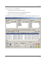
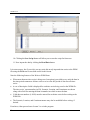
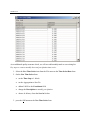
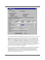
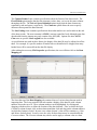
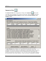
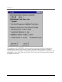
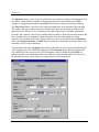
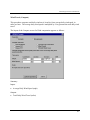
Lesson 1: Introduction, WDM Open, and Time-Series Selection
In this lesson, WDMUtil will be started and a WDM file opened. The main WDMUtil form will
be explored along with the help system. Exercises will then show different methods for selecting
time-series data of interest for further review and analysis. Upon starting WDMUtil, the main
form appears:
The main WDMUtil form is divided into a menu bar and six frames including Scenarios,
Locations, Constituents, Time Series, Dates, and Tools. Each of the six frames is named in the
upper left corner.
At any time when WDMUtil is being run, the complete manual is available online. To access the
manual, simply press the F1 key. This command brings up the WDMUtil online manual open to
a section appropriate to the current situation.
10
Tutorial
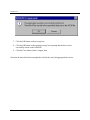
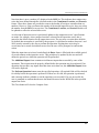
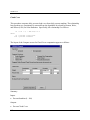
Key Steps to Open an existing WDM file:
1. Select the Open menu item from the File menu.
2. Select the Sample folder to move to the sample data directory.
3. Select sample.wdm to open the sample WDM file.
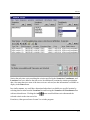
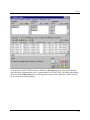
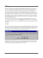
The WDM file is read and the main WDMUtil form is updated with the sample data as shown:
11
WDMUtil 2.0
The Scenarios, Locations, and Constituents frames contain lists of all scenarios, locations, and
constituents found on the time series in the WDM file. When a WDM file is first opened, all of
the time series on the WDM file are added to the list in the Time Series frame. This list displays
information about the time series that meet the criteria in the Scenarios, Locations, and
Constituents lists. This frame also contains a toolbar for managing the contents of the timeseries list.
The Dates frame contains information about the range of dates available that is common to the
currently selected time series. For our selected time series, data are available from January 1,
1980, to December 31, 1982.
The Tools frame contains a toolbar that operates WDMUtil’s analysis and computational tools.
Later lessons will describe how to use these tools.
Between the Scenarios, Locations, and Constituents lists and the Time Series list, there is an
invisible line, which may be used to resize these lists. This line is indicated by the mouse pointer
changing to an up/down arrow when the pointer passes over the line. Resizing is performed by
clicking on the line and dragging it up or down to adjust the list sizes as desired. Additionally,
the entire main form of WDMUtil may be resized by dragging the edges of the form.
Resume this lesson by clearing the time-series list. This is done by clicking on the Clear
button in the Time Series frame. The filtering capability of the Scenarios, Locations, and
Constituents lists will now be demonstrated.
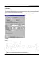
Key steps to find which locations have precipitation data:
1. If the time-series list is populated, clear it by clicking the Clear
button.
2. Click on the PREC item in the Constituents list.
3. Leave the Scenarios and Locations lists with no selections (this is equivalent to selecting
all items in those lists).
4. Click on the Add
12
button in the Time Series frame.
Tutorial
Notice that only time series matching the criteria specified in the Scenarios, Constituents, and
Locations lists were added to the time-series list and that all locations do contain precipitation
data. Also note that since none of the time series are selected, no date information is available to
display in the Dates frame.
In a similar manner, we could have determined what data is available at a specific location by
selecting that location from the Locations list and leaving the Scenarios and Constituents lists
with no selected items. Clicking the Add
selected criteria to the time-series list.
button would add time series that match the
From here, either proceed on to Lesson 2 or exit the program.
13
WDMUtil 2.0
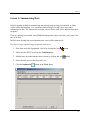
Lesson 2: Importing External Data to a WDM File
This lesson will demonstrate the most fundamental need addressed by WDMUtil, that is, taking
data not on a BASINS WDM file and adding it to that WDM file for use in BASINS. How to
import data into WDMUtil and store it on a WDM file will be demonstrated. If you haven’t
already, begin this lesson by opening the sample.wdm file.
All time series are read into WDMUtil using a data import scripting language. A user interface,
or wizard, for developing data import scripts is included in WDMUtil and will be shown later in
this lesson. When a file is specified to be imported, a list of available scripts is displayed. If the
user knows that a specific script will properly process the data being imported, as is usually
indicated with a green highlight, they may select that script and run it to read the data. If no
script exists for the data being imported, the wizard may be used to develop a new script or the
user may develop the script with a text editor. Examples of importing data with an existing
script and by developing a new script are shown here.
A common need in applying BASINS is to update existing WDM data with more recent values.
For this example, we will import precipitation data and append it to an existing time series, ID
number 201.
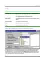
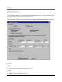
Key steps to Import a time series for which a data import script exists:
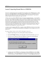
1. Begin the importing process by selecting the File:Import menu item.
2. From the File Import dialogue, select the NCDC export file named ithaca_prec.ncd.
3. If you have yet to import any data into WDMUtil, a message box will be displayed
informing you of the need to load scripts into the system.
4. Loading scripts into WDMUtil is performed by clicking the Find button on the Script
Selection form. Scripts distributed with WDMUtil can be found in the /scripts directory
below the directory in which WDMUtil was installed. Click the Find button and in the
14
Tutorial
File Open dialogue move to the /scripts directory. For this exercise, we will be using the
script in the file HPCP_NCDC_Arch.ws, so select it from the dialogue.
5. From the Script Selection form, note that the HPCP_NCDC_Arch.ws script has a green
background and is selected.
6. Click the Run button.
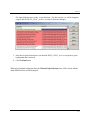
When it has finished reading the data, the Wizard Script Selection form will be closed and the
main WDMUtil form will be displayed.
15
WDMUtil 2.0
Note that the main form has been updated to reflect the newly read time series. Various elements
of the Time Series frame have been updated, such as the counts of available time series and time
series not on the WDM file, and the list of time series. Note that the new time series has a Type
of In-Memory instead of WDM and that it is displayed in a color different from the WDM time
series. This new time series is now available to WDMUtil, in the same manner as existing
WDM time series, for analyses and computations. However, it is not yet saved on the WDM file.
As with any computer work, saving should be performed when significant changes are made. In
this case, we have gone through the effort of importing a time series. If this time series is to be
stored on the WDM file, it is advisable to perform this operation now. If imported time series
are not saved on the WDM file and WDMUtil is exited (or the WDM file is closed), a message
box will be displayed confirming that the user wishes to exit without saving the data.
16
Tutorial
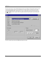
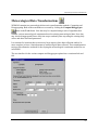
Key steps to Save time series to a WDM file:
1. Select the time series to be saved on the WDM file, in this case the In-Memory time
series just imported.
2. Click the Write
button in the Tools frame.
3. On the Write to WDM form, enter the ID number for the existing time series to which the
newly imported data will be appended, ID number 201.
4. Click the Write button. Since the output time series already exists, a message box will
ask what you would like to do with the data being saved. As we wish to append the new
data to the existing time series, click the Append button.
5. A message box informs you that the data was successfully appended.
There is frequently a need for localized data when a study site is not near a station stored on the
original BASINS WDM file. To continue the example, we will import some evaporation data for
a new location. However, the data being imported is in a format that no existing script can
process. In this case, we will have to develop a new script using the script wizard.
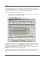
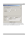
Key steps to Import a time series for which no data import script exists:
1. Begin the importing process by selecting the File:Import menu item.
2. From the File Import dialogue, select the file named Ith_wind.exp.
3. From the Script Selection form, select the Blank Script and then click the Edit button.
17
WDMUtil 2.0
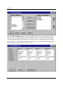
4. On the Input Wizard form, note the Header frame that is used to skip header lines at the
start of a file. In this frame, click the Lines option and specify to skip 1 line.
5. The remaining frames, used to specify the Column Format and Line Ending properties,
are defaulted to Fixed Width and CR/LF or CR, respectively. These are appropriate for
the file being imported. Now click on the Data Mapping tab at the top of the form.
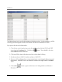
6. The list at the top of the Data Mapping tab contains names of various data elements used
in importing data. On this list, click on Value to begin defining the columns in which the
data values are found. Above the frame displaying the data file is a row of column
numbers. These column numbers can be highlighted, by clicking and dragging with the
mouse, to define the location of the data elements. Now define the location of the data
values by highlighting columns 14 - 24. The Input Column numbers for the Value
element will then be updated in the data elements list.
18
Tutorial
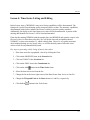
7. In the same manner, define the columns for the Year (1 - 4), Month (6 - 8), and Day (10 12) data elements.
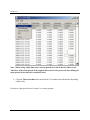
8. Since these are daily data, set the Hour data element to a constant value of 24 by entering
24 under the Constant column.
9. For the Scenario, Location, Constituent, and Description elements, click under the
Constant column and enter text descriptions for these elements (e.g. OBSERVED,
ITHACA, WIND, Daily wind at Ithaca).
19
WDMUtil 2.0
10. Clicking the Save Script button will allow you to store the script for future use.
11. Now import the data by clicking the Read Data button.
It is not necessary, but if you wish, you may write this newly imported time series to the WDM
file using the Write tool as was done earlier in this lesson.
Note the following features of the Write to WDM form:
•
When more than one time series is being saved, an option is provided to save only the data in
the time period common to all time series or to save the full period of data for each time
series.
•
A row of descriptive fields is displayed for each time series being saved to the WDM file.
The time series’ current number (or ID), Scenario, Location, and Constituent are shown
along with a field for entering the data-set number on which to store the data.
•
Valid data-set numbers (1-9999) must be entered for each time series before writing to the
WDM file.
•
The Scenario, Location, and Constituent names may also be modified before writing, if
desired.
From here, either proceed on to Lesson 3 or exit the program.
20
Tutorial
Lesson 3: Summarizing Data
In this lesson the method for summarizing data and reporting missing, accumulated, or faulty
values will be demonstrated. It is common to find missing or invalid values in recorded
meteorological data. The Summarize tool helps a user to locate such values and determine their
frequency.
If you are starting from scratch, start WDMUtil and open the sample.wdm file, (see Lesson 1 for
how to do this).
In this lesson, missing data in precipitation time series will be summarized.
Key steps to begin summarizing precipitation time series:
1. If the time-series list is populated, clear it by clicking the Clear
button.
2. Select only the HPCP item from the Constituent list.
3. Add the time series that matches these criteria by clicking the Add
button.
4. Select the time series in the time-series list.
5. Click the Summarize
button in the Tools frame.
21
WDMUtil 2.0
For the data used in this exercise, it is known that our missing value indicator is -9.99 and our
missing time distribution indicator is -9.98. These are common values for precipitation data. For
other meteorologic data, missing values are often indicated by a value of -999.
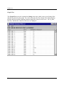
Key Steps to Perform Summary of the time series:
1. Modify the values in the Specifications frame as needed: Miss. Val. = -9.99, Miss. Dist.
= -9.98, Faulty Min = -1, Faulty Max = 10000.
2. Click the Perform Summary button.
The Details frame displays a list of each missing data period, the date and time that it starts, and
the number of time intervals in it. The Summary frame displays total number of periods and
time increments of missing values, missing distributions, and faulty values.
If desired, the Save Summary button may be used to output the contents of the Details and
Summary frames to a file for future viewing or printing.
The following lesson (Time-Series Listing and Editing) will demonstrate how to list time series
with missing values along-side time series with good values and how to edit these missing
values.
22
Tutorial
Lesson 4: Time-Series Listing and Editing
In this lesson, some of WDMUtil’s time-series listing capabilities will be demonstrated. The
listing tool is useful for performing quality assurance checks on data. The summary capabilities,
demonstrated in this lesson, enhance the list tool’s ability to assist in quality assurance.
Additionally, the ability to edit listed time-series values will be demonstrated. A portion of the
missing data identified in Lesson 3 will be listed and amended.
If not already running WDMUtil with the sample data, start WDMUtil and open the sample.wdm
file (see Lesson 1 to learn how to do this). We will list the observed precipitation data at
NY000687, or time-series number 31, which is hourly data. However, as a quality assurance
check without looking at every hourly value, we will list the daily sums of this time series’
values to look for any abnormal daily totals.
Key steps to generating a daily listing of hourly data values:
1. If the time-series list is populated, clear it by clicking the Clear
2. Click on the OBSERVED item in the Scenarios list.
3. Click on NY00687 in the Locations list.
4. Click on the PREC item in the Constituents list.
5. Click on the Add
button in the Time Series frame.
6. Select the lone time series from the list
7. Change the list in the lower right corner of the Dates frame from Native to Sum/Div.
8. Change the TStep and Units in the Dates frame to 1 and Day, respectively.
9. Click the List
button in the Tools frame.
23
WDMUtil 2.0
As an additional quality assurance check, we will now add monthly totals to our existing list.
Key steps to create a monthly observed precipitation time series:
1. Select the New Time Series item from the File menu on the Time Series Data form
2. On the New Time Series form:
•
set the Time Step to 1 Month
•
set the Aggregation to Sum/Div
•
addend -MON to the Constituent field
•
change the Description to monthly precipitation
•
choose In-Memory from the Save in list box
3. press the OK button on the New Time Series form
24
Tutorial
Note that the newly created time series of monthly totals is now listed next to the original
observed precipitation data on the Time Series Data form. Also note that the newly created
monthly time series will be available in WDMUtil even after the list is closed. This new time
series will be “In-Memory”, not on the WDM file, and it need not be saved.
25
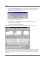
WDMUtil 2.0
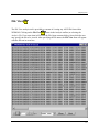
The List tool may also be used to edit missing or faulty data values. For this example we will be
correcting some missing data on time-series number 201 that was identified in Lesson 3.
Key steps to edit time-series data values:
1. Clear all time series from the time-series list and then select both the HPCP and PREC
items from the Constituent list. Click the Add
series added to the time-series list.
button. There should be four time
2. Click on all of the items in the time-series list to select them for listing.
3. Set the start date to 1980/12/1 and the end date to 1980/12/31.
4. Since we will be editing values, we want to make sure we are listing the data at its actual
time interval. Select the Native item from the list in the lower right corner of the Dates
frame.
5. Click the List
December 2nd.
26
button to generate the time-series listing and then scroll down to
Tutorial
6. Note that the first two hours of December 2nd for the ITHACA location contain values of 9.98, which was set as the default value to indicate missing time distributions in Lesson
3. The 3rd hour’s value is 0.05 indicating that the reading measured 0.05 at that hour, but
the event(s) could have occurred any time during the past 3 hours.
7. Based on the values of the nearby stations, it is likely that the event did occur during the
3rd hour. Therefore, the first 2 values on the 2nd can be set to 0 and the 3rd hour’s value
can be left as 0.05.
8. For the purpose of this lesson, it is not necessary to save the edited values. If you did
wish to save the edited valus back to the WDM file, the Save Changed option from the
File menu would be used. WDMUtil would then prompt you for a time-series number to
which the edited values would be saved.
27
WDMUtil 2.0
Note: When saving edited time series, only the period of record in the list will be saved.
Therefore, if the whole period of the original time series is to be preserved after editing, the
entire period of the time series should be listed.
9. Close the Time Series Data form and click the Yes button when asked about discarding
edited values.
From here, either proceed on to Lesson 5 or exit the program.
28
Tutorial
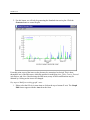
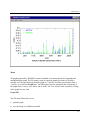
Lesson 5: Time-Series Graphics
In this lesson, some of WDMUtil’s time-series graphics capabilities will be demonstrated. The
Graph tool provides a suite of plots for graphically viewing time-series data. This lesson will use
a standard time-series plot to compare two related time series’ values over time.
If not already running WDMUtil with the sample data, start WDMUtil and open the sample.wdm
file (see Lesson 1 to learn how to do this). We will plot the first two hourly precipitation (PREC)
time series in the Time Series list, numbers 31 and 131. (If these time series are not in the list,
clear the list using the Clear
button, select all items in the Scenario, Location, and
button).
Constituent lists, and then add all the time series using the Add
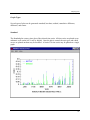
Key steps to Generate a standard time series plot:
1. Select the time series to be plotted from the time-series list. Do so by finding the first
time series (number 31) and clicking on it. Then find the second time series (number
131) and while holding down the Ctrl key, click on it.
2. Since this is hourly data, we will only plot the first three months. So change the change
the starting date to 1/1/1980 and the ending data to 3/31/1980 in the Dates frame.
3. Either set the TUnits list to Hour or set the list in the lower right corner of the Dates
frame to Native.
4. Click the Graph
button in the Tools frame.
29
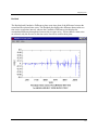
WDMUtil 2.0
5. For this lesson, we will only be generating the Standard time-series plot. Click the
Generate button to create the plot.
From this point, most of the items on the plot may be customized as desired. This is done
through the use of the Edit menu, which has options for modifying Axes, Titles, Curves, General
information, and Lines. Besides using the Edit menu, many of these modifications may be
initiated by clicking on the item to be changed.
Key steps to Modify an existing graph’s axes:
1. Either select the Edit:Axis menu item or click on the top or bottom X-axis. The Graph
Edit form to appear with the Axes tab at the front.
30
Tutorial
2. To have the curves use more of the available plotting space, change the Axis Scale
Range:, Max: value from 0.4 to 0.3. Also change the number of tics from 10 to 6 to have
round numbers on the tic labels.
3. Now click the OK button and the plot will be redrawn with the modified Y-axis scale.
Close the Plot form by clicking the X in the upper right corner (or by selecting the File:Close
menu item). Also close the Graph form by clicking the Cancel button. From here, either
proceed on to Lesson 6 or exit the program.
31
WDMUtil 2.0
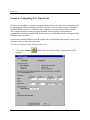
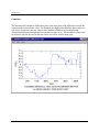
Lesson 6: Computing New Time Series
In this lesson, the ability to compute new meteorological time-series data from existing data will
be demonstrated. When developing a BASINS study for a local area that is not near an existing
BASINS WDM location, it is common to have a limited set of meteorological data available.
The Compute functions provide alternative methods for developing the meteorological
constituents needed for use in BASINS. In this lesson we will demonstrate how to compute Solar
Radiation time-series data.
If not already running WDMUtil with the sample data, start WDMUtil and open the sample.wdm
file (see Lesson 1 to learn how to do this).
Key steps to Compute a Solar Radiation time series:
1. Click on the Compute
displayed.
32
button in the Tools frame and the Compute form will be
Tutorial
2. For each of the six Compute Functions, the Time Series frame prompts for the needed
input and output time series. As indicated, the input data needed to compute Solar
Radiation is Cloud Cover. Leave the input time series’ constituent name as the default,
DCLO.
3. Click on the Constituent list, initially shown as mult. The mult indicates that there is
more than one location that has daily cloud cover data. From the Locations list select the
location NY000687.
4. The combination of Constituent DCLO, Location NY000687, and Scenario OBSERVED
uniquely identifies time series number 42, as is displayed in the DSN (data-set or time
series number) list. As the input time series specifications were made, default values for
the output time series have been supplied. The only remaining item to be specified for the
output time series is its number. Enter 500 in the text field for output DSN.
5. The only required information remaining to be specified is the longitude of the location.
Enter 42, 6, and 0 in the three fields for defining the location’s longitude.
33
WDMUtil 2.0
6. Click the Perform Operation button. A message box will be displayed indicating that
the operation was successful and asking to confirm that the computed data should be
stored on the designated output time series.
7. Click the OK button on this message box.
8. Click the OK button on the ensuing message box reporting that the data set was
successfully stored on the WDM file.
9. Click the Close button on the Compute form.
Note that the main form has been updated to include the newly computed time series.
A second item (COMPUTED) has been added to the Scenarios list since the newly computed
time series’ scenario name was COMPUTED. Scrolling to the bottom of the list in the Time
Series frame will display the new time series. From here, either proceed on to Lesson 7 or exit
the program.
34
Tutorial
Lesson 7: Disaggregating Time Series
In this lesson, the ability to disaggregate existing meteorological time-series data to a new time
series will be demonstrated. When developing a BASINS study for a local area that is not near an
existing BASINS WDM location, it is common to have a limited set of meteorological data
available. Additionally, there is frequently even less available data at the hourly time step
required by BASINS. The Disaggregate functions provide alternative methods for developing
the hourly meteorological data needed for use in BASINS.
If not already running WDMUtil with the sample data, start WDMUtil and open the sample.wdm
file (see Lesson 1 to learn how to do this).
Key steps to Disaggregate daily dewpoint temperature data to hourly dewpoint temperature
data:
1. Click on the Compute
displayed.
button in the Tools frame and the Compute form will be
35
WDMUtil 2.0
2. Select the Disaggregate option in the Operation frame.
3. Select the Dewpoint Temperature option in the Disaggregate Functions frame. The
needed input and output time series are specified in the Time Series frame. The pulldown list next to the Dewpoint Temperature label contains all of the constituent types
from the available time series. Since WDMUtil knows that daily Dewpoint Temperature
data is needed to disaggregate to hourly dewpoint, it has defaulted the list to the DPTP
(daily dewpoint temperature) item.
4. The Locations and Scenarios lists have now been updated to contain only items from
time series that are of daily dewpoint temperature type. The mult displayed in the
Location column indicates that there is more than one location that has daily dewpoint
temperature data. Click on the Locations list and select the first item in the list
NY000687.
36
Tutorial
5. The OBSERVED displayed in the Scenario List indicates that this is the only scenario for
which dewpoint temperature data at location NY000687 exist. The 43 displayed in the
DSN (data-set number) list indicates that a unique time series has been defined by the
selections in the Constituent, Location, and Scenario lists. (If a user knows the number
of the time series needed, they may select it from the DSN first and the Constituent,
Location, and Scenario items will be filled in for that time series.) Note that default
values for the output time series have been supplied as the input time series specifications
were made. The only remaining item to be specified for the output time series is its
number. Enter 501 in the text field for output DSN.
6. The start and end dates, displayed in the Dates frame, reflect the period of available data
in the input time series. Leave the start and end dates as they are and now click the
Perform Operation button. A message box will be displayed indicating that the
operation was successful and asking to confirm that the disaggregated data should be
stored on the designated output time series.
37
WDMUtil 2.0
7. Click the OK button on the message box.
8. Click the OK button on the ensuing message box reporting that the data set was
successfully stored on the WDM file.
9. Click the Close button on the Compute form.
Note that the main form has been updated to include the newly disaggregated time series.
38
Tutorial
A second item (COMPUTED) has been added to the Scenarios list (if it wasn’t there already)
since the newly computed time series’ scenario name was COMPUTED. Scrolling to the bottom
of the list in the Time Series frame will display the new time series. From here, either proceed
on to Lesson 8 or exit the program.
39
WDMUtil 2.0
Lesson 8: Creating a New WDM File
In this lesson, the method for creating a new WDM file will be demonstrated. Creating a new
WDM file allows the user to build a WDM file that contains only the data they desire. The new
WDM file is also likely to be much smaller than existing BASINS WDM files.
Begin by starting WDMUtil (or close the active file if currently running the program) and then
selecting the File:New menu item. A file dialogue form is displayed for specifying the name of
the new WDM file.
Enter NewProj in the text box for the name of the new WDM file. The file dialogue will
automatically add a .wdm extension to the specified file name if the user does not provide it.
Click the Open button to create the new WDM file.
Notice that the caption on the main form displays the base portion of the new WDM file’s name.
The various lists on the main form will be populated as data is read into the system and then
added to the WDM file.
40
Tutorial
End the session by closing WDMUtil. You will notice the new WDM file residing in the
directory in which it was created. You may delete this file after the session is concluded.
41
WDMUtil 2.0
Data Access and Selection
Data accessed by WDMUtil can be grouped into two general categories: WDM data and data in
flat (ASCII text) files. WDMUtil requires a WDM file to be opened (or created) before any
others. Once a WDM file is opened, other flat files containing data external to the WDM file
may then be opened. All data access is initiated through the File menu. Existing WDM files are
opened using the File:Open menu item and flat files are opened using the File:Import menu item.
New WDM files may be created using the File:New menu item.
File
When no WDM file is active, the available menu items under the File menu title are the New,
Open, and Exit items.
42
Data Access and Selection
After a WDM file is open, the available menu items are Import, Close, and Exit.
Once a WDM file is opened, it must be closed in order to open another WDM file or create a
new WDM file.
New
The File:New menu item is used to initiate the process of creating a new WDM file. Creating a
new WDM file allows the user to build a WDM file that contains only the data they desire. The
new WDM file is also likely to be much smaller than existing BASINS WDM files.
Selection of the File:New menu item causes a file open dialogue to appear which allows the user
to enter a name for the new file. The file dialogue will automatically add a .wdm extension to the
specified file name if the user does not provide it. If the file specified already exists, the user will
be instructed to enter the name of a file that does not exist. After specifying the new WDM file
name, the user will be asked to confirm that they want to create the file.
Open
Selection of the File:Open menu item causes a file open dialog box to be opened.
43
WDMUtil 2.0
This dialog box is used to open the desired WDM file. Once the WDM file is opened, the
WDMUtil main form will be refreshed based on the contents of the selected WDM file.
Import
Selection of the File:Import menu item allows the user to access time series data not on the
WDM file and bring it into WDMUtil. From there the imported time series may be saved to the
WDM file and/or analyzed and manipulated in the same manner as WDM time series.
Importing of time series is performed using a scripting language. This language was developed
to handle the wide variety of formats in which time series data are stored. Data import scripts
have been developed to process most of the data formats found to date. However, the system is
dynamic in that new scripts may be created and introduced into WDMUtil.
When the File:Import option is selected, a dialogue prompts the user for the name of the file
containing the data to be imported. Once a file has been specified, the user has the option to
select an existing script from the Script Selection form or to create a new script using the Script
Creation Wizard. Alternatively, the user may also develop a new script by hand using a text
editor and building a script from scratch or modifying an existing script. For other than simple
formats, this method is preferred as the Script Creation Wizard may not be able to successfully
create scripts for complex formats.
44
Data Access and Selection
Details of the Script Selection and Script Creation Wizard forms are presented in the ensuing
sections. Details on the scripting language are presented in the appendix section named
Scripting Language.
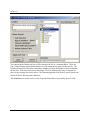
Script Selection
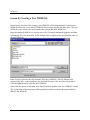
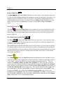
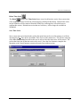
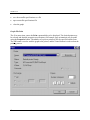
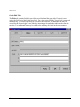
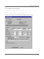
Once a file has been selected for importing, the Script Selection form is displayed.
The form displays all of the data import scripts of which WDMUtil is aware. The list of scripts
contains a column of short descriptions and a column of script file names. Green scripts have
tested the current file and can probably read it. Pink scripts have tested the current file and
probably can’t read it. Red scripts contain errors or cannot be found on disk. Other scripts are
unable to test files for readability.
If a script is green (or you are certain that the script will properly process the data), selecting it
and then clicking the Run button will cause the data to be read and brought into WDMUtil.
If no appropriate script is available, the user has three options:
1. Selecting a script that processes data similar to yours and then clicking the Edit button to
bring up the Script Creation Wizard. From there the script may be modified to process
your data.
2. Selecting the Blank Script item and then clicking the Edit button to bring up the Script
Creation Wizard. From there a new script may be built to process your data.
3. Using a text editor to modify an existing script to process your data.
Note: some complex scripts use features that can not yet be edited in the graphical
interface. These scripts may be edited manually as text files before pressing ‘Run’.
45
WDMUtil 2.0
Clicking the Find button browses your disk for new scripts that are not in the list. The full suite
of scripts distributed with WDMUtil may be found in the /scripts directory under the directory
where WDMUtil was installed.
Clicking the Forget button removes the selected script from the list, but leaves it on disk.
Clicking the Debug button runs the selected script one step at a time. This is a useful tool when
creating new scripts and you want to check each step of the script as it processes the data.
Clicking the Cancel button closes the Script Selection form without importing any data.
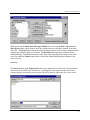
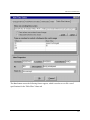
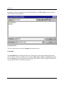
Script Creation Wizard
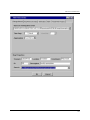
When the Edit button on the Script Selection form is clicked, the Script Creation Wizard is
displayed.
The File Properties tab contains general specifications about the data file being imported. The
name of the file being imported and the name of the script file being edited, along with its
description, are displayed at the top of the form. (If building a new script, the Script File name
will be blank). The Browse buttons to the right of the file names allow different files to be
selected.
The Header frame contains specifications about processing any header lines in the file. If the
Skip check box is checked, there are three options available for skipping header records: None,
lines that Start With a specified character, or a specified number of Lines.
46
Data Access and Selection
The Column Format frame contains specifications about the format of the data records. The
Fixed Width option implies that the data elements (values, dates, etc) are in the same columns
throughout the file. The Tab and Space Delimited options imply that the data elements are
separated by tabs and spaces, respectively. The Character option allows the user to specify
characters that separate the data elements.
The Line Ending frame contains specifications about what markers are used to indicate the end
of the data records. The most common is CR/LF (carriage return/line feed), although some data
downloaded from the internet may only contain a line feed (LF). Options for other ASCII
Characters or specific Line Lenghths are also available.
As specifications are made in these frames, the display of the data file may be adjusted to reflect
them. For example, if a specific number of header lines are identified to be skipped, that many
header lines will be removed from the data file display.
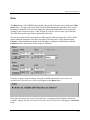
After making the necessary File Properties specifications, the user will then click on the Data
Mapping tab.
The list at the top of the Data Mapping tab contains Names of various data elements used in
importing data. The lower portion of the tab contains a display of the data file with column
numbers across the top of it. These column numbers can be highlighted, by clicking and
dragging with the mouse, to define the location of the data elements. Thus, to define the Input
Column for a data element, click on that element and then click and drag on the column numbers
in which the element is found. In some cases a data element’s value will be constant (e.g. Hour
and Minute for daily data). In such a case, the value for that element may be entered under the
Constant column. The Constant column may also be used to apply a constant value to a data
47
WDMUtil 2.0
element. This is done by inserting the desired mathematical symbol in front of the constant
value. For example, if the year values on a file were only the last two digits, entering +1900 in
the Constant column would add 1900 to the 2-digit year values when processing the data.
Some data elements are general information about the data being processed. These elements
may be stored as attributes of the time series. To indicate a data element as an attribute, a yes is
entered under the Attribute column for that element. The values for these attributes may then be
entered under the Constant column. It is important to enter values for the Scenario, Location,
and Constituent attributes as this will make the new time series more recognizable by WDMUtil
and other BASINS components.
Once the data elements have been defined as desired, the Save Script button may be used to
write the script to a file for future use. The Read Data button is used to try to process the data
using the script defined in the wizard. The Cancel button will close the Wizard and no data will
be imported.
Close/Exit
The File:Close and File:Exit menu items close the currently active WDM file. The File:Exit item
additionally shuts down the WDMUtil system. During the WDM file closing, WDMUtil checks
to see if there was data read in that has not been saved to the WDM file. If there is, the user is
asked whether or not they want to close or exit without saving the data.
Clicking the No button will return the user to the main form so that they may Write the data to
the WDM file. Clicking the Yes button will close the WDM file without saving the data. If the
File:Exit menu item was selected, WDMUtil will be shut down.
48
Data Access and Selection
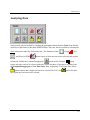
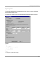
Scenario, Location, Constituent Lists
The Scenarios, Locations, and Constituents frames of the main WDMUtil form display
available and selected items associated with the time series that are known to WDMUtil. The
summary label in the upper left corner of the frames shows a count of the items that are selected
and available. The All button is used to select all available items. The None button deselects all
items. The list of available items is in alphabetical order with selected items highlighted.
49
WDMUtil 2.0
Time Series
The Time Series frame of the WDMUtil form displays a list of the time series selected for
analysis.
For any time series to be available to WDMUtil, three attributes must be present - constituent,
location, and scenario. A toolbar and a corresponding menu title are provided to allow the user to
manipulate the time-series list in a variety of ways. In the top left corner of the frame, the
number of time series in the list is displayed along with the number of time series available in
this project.
Each row in the list contains the attributes of one time series. To select a single time series, click
on the corresponding row. There are two ways to select multiple successive time series in
succession. The first step for both is to select the row representing the first time series. The next
step is to either: 1) continue to hold down the left mouse button from the first selection and drag
the mouse arrow to the row representing the last time series, or 2) hold down the Shift key and
select the row representing the last time series. Multiple time series out of succession can be
selected by holding down the Ctrl key while making the selections. To select all rows, click the
All button in the top right corner of the frame. To deselect all rows, click the None button.
If there are any time series in the list, fields displaying the available dates will automatically
appear in the Dates frame below the Time Series frame. Initially, the Dates frame includes the
starting and ending dates of the period common to all time series in the list. If the Common
button is clicked, then the union of the starting and ending dates for all time series in the list are
displayed.
50
Data Access and Selection
Add Time Series
The Add
button in the Time Series frame is used to add items to the time-series list.
Available time series that meet the selected scenario, constituent, and location selections will be
added. For example, if the user has selected OBSERVED from the Scenarios list, PREC from the
Constituents list, and All from the Locations list, all OBSERVED time series with precipitation
data will be added.
If no items are selected in either the Scenarios, Locations, or Constituents frame when the user
clicks the Add button, then all items in that frame are considered for addition to the time-series
list (i.e., having no items selected from one of these frames is the same as having all items
selected). For Example, if the user has selected OBSERVED from the Scenarios list, PREC from
the Constituents list, and has made no selections from the Locations list, then the same time
series as shown above will be added to the list.
51
WDMUtil 2.0
Remove Time Series
The Remove
button in the Time Series frame is used to remove items from the time-series
list. The text in the left-most column of the list must be selected for that item to be removed. For
example, to remove OBSERVED PREC at NY000687, click on the text WDM in the left-most
column for that list item to select it, and then click on the Remove button. Multiple time series
can be removed at once by highlighting several list items and then clicking on the Remove
button.
Clear Time Series List
The Clear
button in the Time Series frame is another way to remove items from the timeseries list. This button removes all time series from the list if none are selected. If one or more
time series are selected, this button removes the selected time series plus all of the time series
below it on the list.
Move Time Series Up and Down
buttons in the Time Series frame are used to move items in the time-series
The Move
list up or down in the list. The order of the time series in the list is of particular importance for
the Duration and Compare analyses.
These buttons require one item in the time-series list to be selected. A list item may be selected
by clicking on the text for that item in the left-most column. Clicking on the arrow pointing up
will move that item up one place in the list, while clicking on the arrow pointing down will move
that item down one place in the list. Clicking on the first double arrow moves a selected time
series to the top of the list.
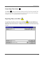
Columns
The Columns
button in the Time Series frame is used to specify which attributes of items
in the time-series list will be displayed as columns in the grid. Clicking on this button produces
a Time-Series Columns form that may be used to manage the columns of the list. The form
contains an Available Columns and Show These Columns list. Individual items are moved
from one list to the other by selecting a list item and then clicking on the Add button or Remove
button. All items can be added to or removed from the Show These Columns list by clicking on
the Add All or Remove All buttons, respectively. There are nine default attributes: Type - file
type as indicated by file name extension File - file name without path or extension DSN - data
set number Scenario - selected item from Scenarios frame Location - selected item from
Locations frame Constituent - item selected from Constituents frame Start - beginning date of
time series End - ending date of time series Nval - number of data values in time series Station
Name - name of the U.S.G.S. meteorological station
52
Data Access and Selection
When an item in the Show the Following Columns list is selected, the Move Up button and
Move Down button can be used to move the column relative to the other columns of the timeseries list. The Reset button returns the selected columns and the order of these columns to their
original state when the form was invoked. The Default button returns the columns to their
default positions. The OK button removes this form while applying these changes to the timeseries list, while the Cancel button removes this form without applying these changes to the
time-series list.
Save List
The Save List item in the Time Series frame on the main menu is used to save the items in the
time-series list to a buffer file for later use. Selecting this menu option invokes the file save
common dialog, from which a user may specify the file name to which this list is to be saved.
53
WDMUtil 2.0
Get Buffer
The Get List item in the Time Series frame on the main menu is used to retrieve items in the
time-series list from a file. Clicking on this button invokes a common dialog that is used to
specify the file name from which this list will be opened.
This feature is designed so that a user might retrieve a list of items for the time-series list saved
previously to a file. The scenario, location, and constituent specifications are read from the file;
and if a time series is available with those attribute values, it will be added to the time-series list.
Edit Time Series Attributes
button in the Time Series frame is used to edit the attributes of items in the timeThe Edit
series list. One or more list items must be selected before clicking on this button.
The Edit Time-Series List form lists the attributes of each selected data series number (DSN).
The Add Attribute button creates an empty row at the bottom of the table. Double-clicking the
Attribute field in this row displays a list box with the attributes that may be added to the DSN.
The OK button removes this form while applying these changes to the time series, while the
Cancel button removes this form without applying these changes to the time series.
54
Data Access and Selection
Delete Time Series
The Delete
button in the Time Series frame is used to delete time series. One or more time
series in the time-series list must be selected before clicking on this button. Deleted time series
on the WDM file will be removed from the WDM file (a message box will ask the user to
confirm this action). Deleted time series that are In-Memory will no longer be available in
WDMUtil.
Save Time Series
One or more time series listed in the grid on the main form can be saved in memory or to file by
choosing the Save Time Series item under Time Series on the main menu. The list box at the top
of the Save Time Series form allows the user to select where the time series will be stored. The
grid on the form lists all the time series to be saved. Press the Save button to complete the
operation or the Cancel button to return to the main form without saving.
55
WDMUtil 2.0
New Time Series
The user can create a new time series by choosing the New Time Series item under Time Series
on the main menu. This function can also be accessed by clicking the Generate Time Series
button on the Analysis toolbar. Either method invokes the New Time Series form shown
below.
The properties of the new time series are specified in the New Properties frame at the bottom of
the tab. The Scenario, Location, Constituent, and Description fields default to the
corresponding properties of the selected time series. If no time series is selected, these fields are
blank. The user may edit any of these fields. The ID field assigns a unique numeric
identification to the time series; therefore, ID values for existing time series in the active project
can not be reused. The ID is equivalent to the Data Set Number (DSN) of a time series stored in
a .wdm file. The Save In list box allows the user to choose whether the new time series will be
stored temporarily in memory or permanently to a WDM file.
56
Data Access and Selection
There are five general processes by which the user may create a new timeseries, and each
process has its own tab at the top of the form.
Tab
Description
Change Interval
Changes the time step interval (i.e., day to month) for a time series
listed in the Time Series frame of the main form.
Add/Remove Dates
Modifies time span and/or time interval of existing time series, or
Creates completely new time series with specified time span and
interval.
Shift Dates
Transposes time series forward or backward in time.
Math
Performs mathematical operations on select arguments, which can
be either manually entered or chosen from existing time series.
Table Filter Values
Modifies values in an existing time series that are within a
specified range.
57
WDMUtil 2.0
Change Interval
In order to change the time-step interval for an existing timeseries, click on the Change Interval
tab on the New Time Series form. The existing time series is selected from the list box at the top
of this tab. The new time-step interval is specified in the Time Step fields. The Aggregation
field determines how values are assigned to the new time series. The values assigned by each
aggregation option depend on whether the new time step has the same, a lower, or a higher
frequency than the native time step.
Aggregation Option
New Time Step Is More Frequent
New Time Step Is Less Frequent
Aver/Same
existing or nearest existing values
assigned to the new time series
the average of existing values in
that time interval are assigned to
the new time series
Sum/Div
nearest existing values are scaled
down by appropriate factor to yield
same total value over period of
existing time step
existing values are summed over
period of new time step
Max
Nearest existing value is assigned
to new time series
Maximum existing value within
corresponding period of existing
time step is assigned to new time
series
Min
Nearest existing value is assigned
to new time series
Minimum existing value within
corresponding period of existing
time step is assigned to new time
series
Edit the New Properties frame then click the Ok button to add a new time series to the Time
Series list on the main form. Click the Cancel button to return to the main form without
completing the operation.
58
Data Access and Selection
59
WDMUtil 2.0
Add or Remove Dates
The Add/Remove Dates tab on the New Time Series form allows the user to create a new time
series with a constant time-step interval over a specific time span. The new time series can either
be based on an existing time series or created entirely from scratch. This determination is made
by selecting one of the two radio buttons at the top of the form.
When the Base on existing time series radio button is selected, the baseline time series is
selected from the list box underneath that radio button. The interval of the new time series is the
same as the existing time series. The New Start and New End date frames determine the period
of the new time series.
When the Specify Interval radio button is selected, the desired interval is set in the fields to the
right of that radio button. There is no need to have a time series selected for this option. Again,
the New Start and New End date frames will determine the period of the new time series.
The four options for inputting values into the new time series are contained in the Added Values
frame. If Specify Interval has been selected, only the Set added values to option is available.
Set added values to
Sets all new time series data to this user-entered value.
Copy nearest existing
value
Sets new time series data to the nearest chronological value in the
existing time series
Interpolate from nearest
value to
Sets new time series data by interpolating between the nearest
chronological value in the existing time series and the user-entered
value.
Clone existing values
starting at
Sets new time series data by transposing values in time from the
existing time series, beginning at the user-specified date, to the
period of the new time series.
Edit the New Properties frame then click the Ok button to add the new time series to the list on
the main form. Click the Cancel button to return to the main form without completing the
operation.
60
Data Access and Selection
61
WDMUtil 2.0
Shift Dates
In order to shift the starting and ending date of an existing time series backward or forward in
time, select the Shift Dates tab on the New Time Series form. Choose the existing time series
from the list box at the top of the form then type in the desired New Start date. Edit the New
Properties frame then click the Ok button to add the new time series to the list on the main form.
The Dates frame may need to be updated by the user to include the range of the new time series.
62
Data Access and Selection
Math
In order to use a mathematical operation to convert data in an existing time series, select the
Math tab on the New Time Series form. Click the radio button of choice from the list of radio
buttons at the top of the form. The resulting computation is summarized in the light gray label
beneath the radio buttons. The actual arguments for the computation are specified in the list at
the bottom of the tab. Double-click the fields next to the arg1, arg2, etc... Existing time series
can be selected as arguments or the user can type in a numeric value.
The final mathematical option in the list of radio buttons is Interpolate. The arguments for this
option have special meanings. At least on time series must be selected as an argument. The
interpolate function looks for missing values in this time series and replaces them by
interpolating between the chronologically nearest values. Numerical arguments are used to
signal missing values in the time series (i.e., a common value for missing data in a time series is 999 so that value would be entered as an argument). If more than one time series is selected, the
63
WDMUtil 2.0
period of the new time series is set equal to the union of the periods of all the time series
excluding the first.
Edit the New Properties frame then click the Ok button to add the new time series to the list on
the main form. Click the Cancel button to return to the main form without completing the
operation.
Table Filter Values
In order to reassign values within defined numeric ranges of an existing time series, select the
Table Filter Values tab. Choose the existing time series from the list box at the top of the form.
Values are reassigned by one of two methods:
•
The New values are constant in each range radio button reassigns values within a defined
range to a single value
•
The Interpolate between new values radio button reassigns values by interpolating between
two values that represent contiguous ranges
Values are entered in the Values <= column of the grid on this tab by clicking a cell then typing
in a value. Values are entered in the New value column by double-clicking a cell then: 1)
selecting either the Delete or Leave Unchanged list item, or 2) typing in a value. The most
orderly way to complete the grid is to begin with the lowest range at the top of the form and add
each successively higher range on the ensuing line. For the grid shown in the picture below, all
values <=5000 are left unchanged and all values up to 999,999 are rounded down to 5,000. Edit
the New Properties frame then click the Ok button to add the new time series to the list on the
main form. Click the Cancel button to return to the main form without completing the operation.
64
Data Access and Selection
The Save button causes the following form to appear, which is used to save to file a set of
specifications for the Table Filter Values tab.
65
WDMUtil 2.0
Text entered in the Header text box will be written to the file as a comment block. There are
four Column Format options that determine how the output data is spaced in the text file. The
Include Column Titles check box determines whether or not the list headers will be included in
the text file. If the user enters text in the Empty Cell Text field then this entry will appear in
place of any missing time series values. The remaining portion of the form is used to specify the
output file drive, directory path, and name.
The Load button is used to retrieve a set of specifications that was previously saved to a file.
66
Data Access and Selection
Dates
The Dates frame of the WDMUtil form displays the period of the time series listed in the Time
Series frame. The upper white date fields represent the Current time span that will be used in
the analysis operations. The user may change the starting and ending dates for the analysis by
clicking in one of these text boxes. After clicking in a text box, the user may type in the date.
The entire date must be specified (no partial dates allowed).
The lower, gray date fields represent the available period of the listed time series. These fields
display either the common or the entire date range of the time series. If the button beneath
Current is labeled All then the union of all date ranges is displayed. If the button is labeled
Common then the intersection all date ranges is displayed.
If no time series are in the list, dates will not be available. Instead, the text No dates are
available until Time Series are Selected will appear in the Dates frame.
If the time series in the time-series list do not have a common period, then dates will not be
available. Instead, the text No Common Period for Selected Time Series will appear in the Dates
frame.
67
WDMUtil 2.0
The default time step for the listed time series is native, meaning every value in the time series is
included, resulting in possibly irregular time steps. The time step can be set to a constant time
interval by selecting any option other than Native. When the time step is set to a constant time
interval, the TStep,Units field is activated, and the user may then select the constant time
interval.
The Reset button changes the values in these fields back to their defaults.
68
Analyzing Data
Analyzing Data
Analysis tools may be invoked by selecting the appropriate button from the Tools frame located
in the lower right corner of the main WDMUtil form. They may also be invoked by selecting one
of the menu items under the Tools menu title. The Summarize Data
, and Write to WDM
, Graph
, List
options require at least one time series to be selected in order
option nor the Generate
option
to function. Neither the Compute/Disaggregate
require any time series to be selected as the time series selections, if necessary, are made from
the Compute/Disaggregate or New Time Series form, respectively. The Export Time Series
option requires that a single time series be selected. The File View
not require any time series to be selected.
option also does
69
WDMUtil 2.0
Summarize Data
The Summarize Data form is displayed by clicking on the Summarize
button in the
Tools frame or by selecting the Tools:Summarize menu item. The form is composed of three
frames (Specifications, Details, Summary) and three buttons (Perform Summary, Save
Summary, Close).
The Specifications frame contains a row of specifications for each time series being
summarized. The first three columns are to help the user in identifying each time series and are
not editable. The next two columns are used for defining missing value and missing time
distribution (accumulated value) indicators. Time series read in using a data import script may
have specified the values of these indicators. In any case, the user is responsible for defining
70
Analyzing Data
them here. The final two fields are used for defining a minimum and maximum range outside of
which values for the given constituent would not be valid.
The Details frame contains a scrollable text box that reports each instance of missing,
accumulated, or faulty data. For each instance, the number of time intervals, the type of problem,
and the date after which it begins are reported. If a time series has no missing data, a message
indicating such is displayed.
The Summary frame contains a row of information for each time series summarized. The first
two fields indicate the data-set number and the total number of time intervals that were
summarized. The next two fields display the total number of periods (or instances) of missing
values and the total number of time intervals in those periods. Similar totals are reported for
missing time distributions and faulty values in the ensuing fields.
The Perform Summary button is used to generate the missing data summary. The time series
selected from the main form will be scanned for missing, accumulated, and faulty data over the
period specified in the Dates frame on the main form.
The Save Summary button is used to output the details and summary information to a file for
printing and long-term storage.
The Close button is used to remove the form.
71
WDMUtil 2.0
List
The Time Series Data form is displayed by clicking on the List
button on the Analysis
toolbar or by selecting the Analysis:List menu item. The initial listing contains values for the
selected time series displayed at the time interval and for the time period specified in the Dates
frame. All lists generated by WDMUtil contain a standard set of menu items for outputting and
manipulating the list. The File menu title is used to:
•
create a new timeseries to add to the list
•
save edits to all or selected timeseries on the form
•
output the listed values to a text file or printer
•
close the Time Series Data form
The Edit menu title is used to:
•
copy and paste all or selected portions of the list
•
edit the date and number format
•
select and edit timeseries attributes that appear in the list header
72
Analyzing Data
List File
New Time Series
Invokes the New Time Series form. The resulting time series is
added to the list once created by the user.
Save Changed
Saves the changes made to all listed time series
Save Selected
Saves the changes made to the time series in the currently selected
column
Save Text to File
Saves the list to an ASCII text file
Print
Sends the list to the a selected printer
Close
Closes the Time Series Data form
When the Save to Text File option is selected, the following form is displayed.
There are four Column Format options that determine how the output data is spaced in the text
file. The Include Column Titles check box determines whether or not the list headers will be
included in the text file. If the user enters text in the Empty Cell Text field then this entry will
appear in place of any missing time series values. The remaining portion of the form is used to
specify the output file drive, directory path, and name.
73
WDMUtil 2.0
The Print menu item causes the Print dialogue form to be displayed. The desired printer may be
selected and detailed properties specifications (for example, page orientation) may be made
using the Properties button. The number of copies to print may also be specified on this form.
The OK button is used to send the list to the printer, and the Cancel button is used to abort the
printing process.
The Close menu item removes the List form from the screen.
74
Analyzing Data
List Edit
Copy
Copies selected portions of the list to the clipboard
Copy All
Copies the entire list to the clipboard
Paste
Pastes the contents of the clipboard onto the selected portion of the
list
Date Format
Sets the format for date fields in the list
Number Format
Sets the format for data fields in the list
Select Attributes
Determines which of the time series attributes will be displayed as
headers for the list
Edit Attributes
Edits the time series attributes to be displayed as headers for the list
When the Date Format option is selected, the Date Format form is displayed. The format
options on this form are self-explanatory and are applied to all listed date values.
75
WDMUtil 2.0
When the Number Format option is selected, the first three lines of each list column are
dedicated to specifying the Number Width, Significant Digits, and Decimal Places to be
displayed for each value in that column.
76
Analyzing Data
When the Select Attributes option is selected, the Time Series Attributes form appears. The
user can select which attributes of the listed time series are to be included in the list header. In
order to select an item from a list, either double-click on the item, or single-click on the item then
click the Add or Remove button. To add all of the Available areas to the Selected list, click the
Add All button. To return all of the areas from the Selected list to the Available list, click the
Remove All button.
77
WDMUtil 2.0
When the Edit Attributes option is selected, the Edit Time Series List form appears. The user
can type in new text descriptions or numeric identifiers for the various timeseries being listed.
The Add Attribute button at the bottom of the form creates a new attribute associated with the
listed time series. A blank line at the bottom of the form is created to facilitate manual entry of
the attribute name and its value for each time series.
78
Analyzing Data
Graph
The Graph tool allows the user to generate a variety of plots for graphically viewing time-series
data. All of the plots are based on time-series data, but only the Standard, Bar Chart, Residual,
and Cumulative Difference, plots are time plots. The Difference and Scatter plots are x-y plots.
The Standard plot will plot a single or multiple time series at one time. The Bar Chart plot will
display two or more time series side by side over time. The remaining comparison plots use only
two time series. If more than two time series are selected for plotting, only the first two will be
used when generating the comparison plots.
Time plots (standard, bar chart, residual, and cumulative difference) can be plotted at time
intervals other than the time series’ native time steps, which includes every value in the time
series despite possibly irregular time steps. The time interval for the plots is specified in the
Tstep,Units fields in the Dates frame. Available time interval aggregation/disaggregation
options include summing, averaging, dividing, reporting the minimum or maximum value, and
native. To view a chart on how the aggregation options control the resulting plot, see the help
section on changing intervals.
The Graph form is displayed by clicking on the Graph
button in the Tools frame or by
selecting the Analysis:Graph menu item. The Graph form shows the suite of graphs that may be
generated. If there is only one time series selected, then only the Standard plot is available as the
remaining plots require multiple time series. The All button selects all of the available plots for
plotting and the None button deselects them. The Generate button causes all of the selected
plots to be created. The Cancel button closes the Graph form, but will not close any existing
plots.
79
WDMUtil 2.0
All graphs generated by WDMUtil contain a standard set of menu options for outputting and
manipulating the graph. The File menu is used to output the graph to a printer or Windows
metafile and to close the graph form. The Edit menu is used to manipulate the components of the
graph (that is, curves, axes, labels, and so forth). The View menu is used to generate a listing of
the graph in a new form.
80
Analyzing Data
Menu
All graphs generated by WDMUtil contain a standard set of menu options for outputting and
manipulating the graph. The File menu is used to output the graph to a printer or Windows
metafile, save the specifications from this graph to a *.grf file, recall the specifications from a
*.grf file, or to close the Graph form. The Edit menu is used to manipulate the components of
the graph (that is, curves, axes, labels, and so forth). The View menu is used to generate a listing
of the graph in a new form.
Graph File
The File menu allows the user to:
•
print the graph
•
save the image as a Windows metafile
81
WDMUtil 2.0
•
save the metafile specifications as a file
•
open a metafile specifications file
•
close the graph
Graph File Print
The Print menu item causes the Print common dialog to be displayed. The desired printer may
be selected and detailed properties specifications (for example, page orientation) may be made
using the Properties button. The number of copies to print may also be specified on this form.
The OK button is used to send the graph to the printer, and the Cancel button is used to abort the
printing process.
82
Analyzing Data
Graph File Save
The Save menu item causes the Windows Graph Save dialog form to be displayed. The Picture
tab of this form allows the user to save the graph as one of four file types or to copy the picture
to the clipboard. The Specifications tab of this form allows the user to save properties of the
current graph so that those properties can later be recalled and applied to other graphs via the
Open Specification item under File on the main menu of the graph form.
The remaining portion of the form serves the same purpose whether the user is saving the graph
as a picture or saving the graph specifications. The list box at the top of the form specifies the
drive in which to save the file. The middle list box illustrates the path to the current directory on
the specified drive. The Files Matching list box lists the files in the current directory that match
the specified file type. Once the user has selected a file, the File Name list box at the bottom of
the screen will display the full path name of that file.
Open Specifications
The Open Specifications menu item causes the Generate Windows Metafile dialog form to be
displayed. This item allows the user to recall a set of saved properties from a graph file (*.grf)
for application to the current graph. The list box on the top portion of the form is used to specify
the directory path to the graph file. The box in the middle portion of the form displays any
83
WDMUtil 2.0
existing files of the specified type in the specified directory. The File Name text box is used to
enter the name of the graph file.
Graph File Close
The Close menu item removes the Graph form from the screen.
Graph Edit
The Graph Edit form is displayed when any of the first five menu items under the Edit menu
title is selected. The form contains five tabs (Axes, Titles, Curves, Lines, and General) with the
tab corresponding to the selected menu item being in the forefront. When a graph is first drawn it
is given default values for all these parameters.
84
Analyzing Data
Graph Edit Axes
The Axes tab contains radio buttons for selecting the type of X-, Left Y-, and Right Y-axes. An
auxiliary axis is a separate graph above the main graph that shares the same X-axis. A field for
specifying the fraction of the available Y space to use for the auxiliary axis (if it is in use) is also
provided. Each axis frame contains fields for specifying the number of tics and the minimum and
maximum value for the axis. To assist in defining the axis scale, the data range for each axis is
also provided. Should values exceed the axis scale range, the curve will be clipped at that point.
85
WDMUtil 2.0
Graph Edit Titles
The Titles tab contains fields for specifying axes labels and the graph title. If an axis is not
active, the field for its label is also not active. For a time-series plot, the X-axis label is generated
automatically. Up to three lines may be entered for the main title. An additional line may be
created for the left and right Y-axes labels by inserting an & symbol that indicates the start of a
new line. Two additional lines may be added to the auxiliary axis label in the same manner.
86
Analyzing Data
Graph Edit Curves
The Curves tab contains six columns for specifying characteristics of each curve on the plot:
Axis, Line Type, Marker, Color, Value Type, and Legend Entry. Curves can be identified by
their current color. Double-click any field to edit selections. The Axis, Line Type, Marker, and
Value Type columns all contain lists with the available options. A palette with the available
colors will appear for the Color column. The Axis field specifies on which axis the curve is to be
plotted (Left Y, Right Y, Auxiliary). Specifications for line type and thickness, marker type,
color, value type (mean over a time span or point at an instant of time), and legend label may
also be made.
87
WDMUtil 2.0
Graph Edit Lines
The Lines tab contains five columns for specifying characteristics of each line on the graph:
Axis, Line Type, Color, Value, and Legend Entry. A line is distinguished from a curve by the fact
that a curve represents data values while lines merely provide a reference marker (i.e., y=0).
Double-click any field to edit selections. The Axis and Line Type columns contain drop-down
lists with the available options. A palette with the available colors will appear for the Color
column. Values are typed in for the Value and Legend Entry columns.
88
Analyzing Data
Graph Edit General
The General tab contains radio buttons and fields for specifying the location of the legend.
Location options include no legend, the upper left corner (default), and a user-specified location.
Three additional text fields are provided to add any additional text to the plot. Location
specifications for both the legend and the additional text are made by entering the fraction of the
X- or Y-axis (for example, X Position=0.5, Y Position=1.0 means half way across the X-axis and
at the top of the Y-axis).
89
WDMUtil 2.0
Graph View
The Graph View menu title contains the Listing menu item, which creates a text listing of the
data that are plotted on the graph. For a time-series plot, the first column of the listing displays
the date and time and the remaining columns display the values for each curve. For x-y plots,
first the y and then the x data for each curve are displayed.
90
Analyzing Data
Graph Types
Several types of plots can be generated: standard, bar chart, residual, cumulative difference,
difference, and scatter.
Standard
The Standard plot creates a time plot of the selected time series. All time series are plotted on an
arithmetic scale on the left Y-axis by default. Once the plot is created, the axis types and which
curves are plotted on them may be modified. A limit of 18 time series may be plotted on a single
graph.
91
WDMUtil 2.0
Bar Chart
The Bar Chart plot creates a time plot that shows the value from each time series side by side for
each time interval. This plot is intended for close examination of values over a short period of
time. The plot will lose any useful resolution for longer time spans (for example, greater than 50
time intervals).
92
Analyzing Data
Residual
The Residual and Cumulative Differences plots create time plots of the difference between the
second and first selected time series. The Residual plot displays the difference between the two
time series at each time interval, whereas the Cumulative Differences plot displays the
accumulated difference through time between the two time series. If more than two time series
are selected, only the first two in the time-series list will be used for these plots.
93
WDMUtil 2.0
Cumulative
The Residual and Cumulative Differences plots create time plots of the difference between the
second and first selected time series. The Residual plot displays the difference between the two
time series at each time interval, whereas the Cumulative Differences plot displays the
accumulated difference through time between the two time series. If more than two time series
are selected, only the first two in the time-series list will be used for these plots.
94
Analyzing Data
Difference
The Difference plot creates x-y plots using the first two selected time series. The difference
between the two time series is plotted against the first time series. If more than two time series
are selected, only the first two in the time-series list will be used for this plot.
95
WDMUtil 2.0
Scatter
The Scatter plot creates x-y plots using the first two selected time series. The second time series
is plotted against the first. There is an option to display the 45-degree and regression lines on the
plot. If more than two time series are selected, only the first two in the time-series list will be
used for this plot.
96
Analyzing Data
File View
The File View analysis tool is provided as a means of viewing any ASCII file from within
WDMUtil. Clicking on the File View
button in the Analysis toolbar (or selecting the
Analysis:File View menu item) will invoke the File Open common dialog, from which the user
may specify the file to be viewed. After specifying the file name, the File View form will appear
with the file text in a text box.
97
WDMUtil 2.0
The File View form displays files one page at a time. At the bottom of the form is a set of
buttons and a text box that are used to move through the file. The buttons are used to move
forward or backward through the file. The text box is used to enter a specific page number to
which to move. The field to the right of the buttons displays the total number of pages in the file.
An additional list at the bottom of the form allows the user to select the format in which to view
the file. The Plain Text option will fill each page with the maximum amount of text without
using vertical scroll bars. The FORTRAN Output option will perform in this manner also with the
exception that a new page will be formed whenever a FORTRAN carriage control character for
new page is encountered. Although options for viewing in Binary and ESRI Shape File format
exist, they are not used in WDMUtil. This file can be printed using the Print button. The Close
button removes this form.
98
Meteorological Data Transformations
Meteorological Data Transformations
WDMUtil contains two meteorological time-series transformation methods: Computing and
Disaggregating. Both of these methods are accessed by clicking the Compute/Disaggregate
button in the Tools frame. New data may be computed using a suite of algorithms that
estimate various meteorological constituents based on existing meteorological data. New data
may also be disaggregated from a daily time step to an hourly time step using the existing daily
values and other associated parameters.
It is common for locations that are not near a large airport (where data collection tends to be
more complete) to have a limited amount of meteorological data collected. These transformation
tools provide alternative methods for developing the meteorological constituents needed for use
in BASINS.
The user interface for the various compute and disaggregate options has a consistent look and
feel.
99
WDMUtil 2.0
The Operation frame is used to specify whether the user wants to Compute or Disaggregate. The
next frame is named either Compute or Disaggregate Functions and contains the available
compute or disaggregate functions, depending on which type of operation is being performed.
The Time Series frame is used to specify input and output time series needed for the operation.
The number and types of input time series needed varies from one operation to another. Each
input time series will have a row containing a descriptive label, lists of available constituents,
locations, and scenarios, and a list of available data-set numbers. With each selection made in the
lists, remaining lists are updated to contain only those time series that match the current
selections. For example, if the DCLO (daily cloud cover) item is selected from the Constituent
frame, the Location, Scenario, and DSN lists are updated to contain only items from time series
which have DCLO as the constituent.
The mult displayed in the Locations frame indicates that there is more than one location that has
a DCLO time series. The OBSERVED displayed in the Scenarios frame indicates that there are
only OBSERVED time series for the DCLO constituent. The mult displayed in the DSN list
indicates that there are still multiple data sets available for the selections made so far. If one of
the available locations is now selected, a unique time series will be defined.
100
Meteorological Data Transformations
Note that there is now a number (42) displayed in the DSN list. This indicates that a unique time
series has been defined through the selections made in the Constituent, Location, and Scenario
frames. These three frames are provided to remove the burden of having to remember data-set
numbers. However, if the user knows the number of the needed input time series, they may select
the number from the DSN list at any time. The Constituent, Location, and Scenario frames will
be updated to reflect the selected time series.
As selection of input time series is performed, updates to the output time series’ specifications
are made. For example, when a unique location is selected for the input time series, this is
entered as the default location for the output time series. The user may overwrite these defaults.
No default data-set number is specified by the program. A valid data-set number (between 1 and
9999) must be entered by the user to perform the operation. Existing time series may be
overwritten, but to assure desired data are not lost, the user will be prompted to confirm this
action.
When the input time series have been defined, the Dates frame is filled with the available period
of record common to the input time series. This period may be updated by the user and will
define the period over which the operation will be performed.
The Additional Inputs frame contains miscellaneous inputs that are needed by some of the
operations. These inputs must be properly defined before the operation may be performed. If an
operation does not have any inputs other than time-series data sets, the Additional Inputs frame
will not be displayed.
The Perform Operation button starts the specified operation. All required fields will be checked
for validity before the operation is performed. If these are all valid, the operation is performed,
and a message indicates whether or not the operation was successful. If it was successful, the
user is prompted to confirm that the new data should be stored on the WDM file in the specified
output time series.
The Close button will close the Compute form.
101
WDMUtil 2.0
Compute
WDMUtil contains algorithms for computing Solar Radiation, Jensen PET, Hamon PET,
Penman Pan Evaporation, Wind Travel, and Cloud Cover data. The suite of algorithms for
computing these data requires varying numbers and types of existing meteoric time series and
associated parameters. The algorithms and data requirements may be found in the following
sections that describe the different computations.
Solar Radiation (Compute)
This procedure computes the total daily solar radiation based on empirical curves of radiation as
a function of latitude (Hamon et al, 1954). The inputs are latitude in degrees and daily cloud
cover in tenths (ranges from 0 to 10). This method is limited to latitudes from 25 degrees N to
50 degrees N, but this limit is not enforced by the program. The output is total daily solar
radiation at the surface in langleys.
The layout of the Compute screen for Solar Radiation computation appears as follows:
102
Meteorological Data Transformations
Summary
Inputs:
•
Latitude (degrees, minutes, seconds)
•
Daily cloud cover time series (tenths, i.e., 0 - 10)
Output:
•
Daily solar radiation (langleys)
103
WDMUtil 2.0
Jensen PET
This procedure generates daily potential evapotranspiration (inches) using a coefficient for the
month, the daily average air temperature (F), a coefficient, and solar radiation (langleys/day).
The computations are based on the Jensen and Haise (1963) formula.
PET = CTS * (TAVF - CTX) * RIN
where
PET
CTS
TAVF
CTX
RIN
=
=
=
=
=
daily potential evapotranspiration (in)
monthly variable coefficient
mean daily air temperature (F or C), computed from max-min
coefficient
daily solar radiation expressed in inches of evaporation
RIN = SWRD/(597.3 - (.57 * TAVC)) * 2.54
where
SWRD = daily solar radiation (langleys)
TAVC = mean daily air temperature (C)
The following is abstracted from the PRMS manual (Leavesley, et al., 1983): As with the
Hamon procedure, the Jensen-Haise procedure tends to underestimate winter PET; therefore,
monthly variable CTS coefficients are included. Values of CTS and CTX for the warmer months
can be estimated using regional air temperature, elevation, vapor pressure, and vegetation data
(Jensen et al. 1969). For aerodynamically rough crops (assumed to include forests), CTS can be
computed for the watershed by:
CTS = 1/[C1 + (13.0 * CH)]
where
C1 = an elevation correction factor
CH = humidity index
C1 = 68.0 - [3.6 * E1/1000]
where
E1 = median elevation of the watershed (ft)
CH = 50/(e2 - e1)
where
e2 = saturation vapor pressure (mb) for the mean maximum
air temperature for the warmest month of the year
e1 = saturation vapor pressure (mb) for the mean minimum
air temperature for the warmest month of the year
104
Meteorological Data Transformations
CTX is computed for each land segment as:
CTX = 27.5 - 0.25 * (e2 - e1) - (E2/1000)
where
E2 = median elevation of the land segment (ft)
The layout of the Compute screen for Jensen PET computation appears as follows:
105
WDMUtil 2.0
Summary
Inputs:
•
Maximum daily air temperature time series (F or C)
•
Minimum daily air temperature time series (F or C)
•
Total daily solar radiation time series (langleys)
•
Monthly variable coefficient - CTS
•
Constant coefficient - CTX
Output:
•
Daily potential evapotranspiration (inches)
106
Meteorological Data Transformations
Hamon PET
This method generates daily potential evapotranspiration (inches) using air temperature, a
monthly variable coefficient, the number of hours of sunshine (computed from latitude), and
absolute humidity (computed from air temperature). The computations are based on the Hamon
(1961) formula.
PET = CTS * DYL * DYL * VDSAT
where
PET = daily potential evapotranspiration (in)
CTS = monthly variable coefficient
DYL = possible hours of sunshine, in units of 12 hours,
computed as a function of latitude and time of year
VDSAT = saturated water vapor density (absolute humidity)
at the daily mean air temperature (g/cm3)
VDSAT = (216.7 * VPSAT)/(TAVC + 273.3)
where
VPSAT = saturated vapor pressure at the air temperature
TAVC = mean daily air temperature,
computed from the daily max-min data (C)
VPSAT = 6.108 * EXP((17.26939 * TAVC)/(TAVC + 237.3))
Hamon (1961) suggests a constant value of 0.0055 for CTS. However, this has been found to
underestimate PET in some areas, especially for winter months. Therefore, monthly values can
be specified.
The layout of the Compute screen for Hamon PET computation appears as follows:
107
WDMUtil 2.0
Summary
Inputs:
•
Maximum daily air temperature time series (F or C)
•
Minimum daily air temperature time series (F or C)
•
Latitude (D,M,S)
•
Monthly variable coefficient
Output:
•
Daily potential evapotranspiration (inches)
108
Meteorological Data Transformations
Penman Pan Evaporation
This procedure estimates daily pan evaporation (inches) using daily average air temperature (F),
dewpoint (F), wind movement (miles/day), and solar radiation (langleys/day). The method is that
of Kohler, Nordensen, and Fox (1955), and it is based on the Penman (1948) formula; the
following description is abstracted from Hydrocomp (1977):
E = (Q*DEL + Ea*GAM)/(DEL + GAM)
(1)
where
E
= pan evaporation
Q
= net radiation exchange
DEL = slope of the saturation vapor pressure
curve at the air temperature
GAM = 0.0105 inches Hg/deg F (defined by Bowen’s Ratio)
Ea = pan evaporation (assuming air temperature equals
water temperature)
To express the above equation in terms of available meteorological data, empirical curve fitting
of data points is used. An empirical expression for Q*DEL, which can be treated as a single
parameter, is
Q*DEL = exp[(Ta -212) (0.1024 - 0.01066 ln R)] - 0.000
(2)
where
Ta = air temperature (F)
R = daily solar radiation (langleys)
An expression for Ea is
Ea
= (0.37 + 0.0041 Up) * (es - ea)**0.88
(3)
where
(es - ea) = vapor pressure deficit between surface
and dewpoint temperature and
Up = total daily wind movement (miles)
The Clausius-Clapeyron equation can be used to express e, the vapor pressure, and DEL, the
slope of the saturation vapor pressure curve at air temperature Ta:
e = exp{[-7482.6/(Ta + 398.36)] + 15.674}
(4)
DEL = [7482.6/Ta+398.36)**2] exp[15.674-7482.6/(Ta+398.36)] (5)
109
WDMUtil 2.0
To calculate evaporation, the procedure uses Eqn 1. Parameters needed for the evaluation of Eqn
1 are found using Eqns 2-5. Air temperature is estimated as the average of maximum and
minimum daily temperature. If dewpoint temperatures are not available, minimum daily
temperatures can be substituted.
The layout of the Compute screen for Penman Pan Evaporation computation appears as follows:
Summary
Inputs:
•
Maximum daily air temperature time series (F)
•
Minimum daily air temperature time series (F)
•
Average daily dewpoint temperature time series (F)
•
Total daily wind movement time series (miles)
•
Total daily solar radiation time series (langleys)
Output:
•
110
Daily pan evaporation (inches)
Meteorological Data Transformations
Wind Travel (Compute)
This procedure computes total daily wind travel, in miles, from average daily wind speed, in
miles per hour. The average daily wind speed is multiplied by 24 to generate the total daily wind
travel.
The layout of the Compute screen for Wind computation appears as follows:
Summary
Inputs:
•
Average Daily Wind Speed (mph)
Outputs:
•
Total Daily Wind Travel (miles)
111
WDMUtil 2.0
Cloud Cover
This procedure computes daily percent cloud cover from daily percent sunshine. The relationship
between these two constituents is extracted from the algorithms developed by Hamon, Weiss,
and Wilson (1954) for Solar Radiation. Specifically, the relationship is as follows:
CC = 100 * (1 - PSS/100)**0.6
where
CC = percent cloud cover
PSS = percent sunshine
The layout of the Compute screen for Cloud Cover computation appears as follows:
Summary
Inputs:
•
Percent Sunshine (0 - 100)
Outputs:
•
112
Percent Cloud Cover
Meteorological Data Transformations
Disaggregate
WDMUtil contains algorithms for disaggregating Solar Radiation, Temperature, Dewpoint
Temperature, Evapotranspiration, Wind, and Precipitation data. The suite of algorithms for
disaggregating these data requires varying types of existing meteorological time series and
associated parameters. The algorithms and data requirements may be found in the following
sections.
Solar Radiation (Disaggregate)
This procedure distributes daily solar radiation to hourly values by assuming an empirical
distribution over daylight hours that are computed from latitude and time of year. It is limited to
latitudes from 25 degrees N to 50 degrees N, but this limit is not enforced by the program. It is
an empirical method based on work by Hamon et al. (1954).
The layout of the Compute screen for Solar Radiation disaggregation appears as follows:
113
WDMUtil 2.0
Summary
Inputs:
•
Daily solar radiation (langleys or any units)
•
Latitude (D,M,S)
Output:
•
114
Hourly solar radiation (same units as input)
Meteorological Data Transformations
Temperature
This procedure distributes daily max-min temperatures to hourly values; it assumes the minimum
occurs at 6 AM and the maximum occurs at 4 PM.
The layout of the Compute screen for Temperature disaggregation appears as follows:
Summary
Inputs:
•
Maximum daily air temperature (F or C)
•
Minimum daily air temperature (F or C)
•
Observation hour (1-24) - This is the hour at which these max and min temperatures are
recorded. If this hour is 17 - 24, then both the input max and min actually occurred on that
day. If the hour is 6 - 16, then the input max actually occurred on the previous day. If the
hour is 1 - 5, then both the input max and min actually occurred on the previous day.
Output:
•
Hourly air temperature (same as input Min/Max Temperatures)
115
WDMUtil 2.0
Dewpoint Temperature
This procedure distributes average daily dewpoint temperature to hourly values. It assumes that
the daily average is constant over the 24 hour period.
The layout of the Compute screen for Dewpoint Temperature disaggregation appears as follows:
Summary
Inputs:
•
Average Daily Dewpoint Temperature (F or C)
Outputs:
•
116
Hourly Dewpoint Temperature (F or C)
Meteorological Data Transformations
Evapotranspiration
This procedure distributes daily evapotranspiration to hourly values; it assumes a distribution
based on latitude and time of year.
The layout of the Compute screen for Evapotranspiration disaggregation appears as follows:
Summary
Inputs:
•
Daily PET (inches or any units)
•
Latitude (D,M,S)
Output:
•
Hourly PET (same units as input)
117
WDMUtil 2.0
Wind Travel (Disaggregation)
This procedure distributes daily wind movement to hourly values; it allows the user to adjust the
default empirical hourly distribution.
The layout of the Compute screen for Wind Travel disaggregation appears as follows:
Summary
Inputs:
•
Daily wind movement (any length units)
•
Hourly distribution fractions (-)
Output:
•
118
Hourly wind movement (same units as input)
Meteorological Data Transformations
Precipitation
This procedure distributes daily precipitation to hourly values based on hourly time series from
nearby stations. The daily precipitation time series must not contain any missing periods as
indicated by negative values. It distributes the data according to one of several secondary hourly
stations, using the one whose daily total is closest to the daily value. If the daily total for the
hourly stations being used are not within a user-specified tolerance of the daily value, the daily
value is distributed using a triangular distribution centered around the middle of the day.
The layout of the Compute screen for Precipitation disaggregation appears as follows:
119
WDMUtil 2.0
Summary
Inputs:
•
Daily precipitation time series to be disaggregated
•
Up to 5 hourly precipitation time series from nearby stations
•
Observation hour of the daily precipitation time series
•
A data tolerance value representing the allowable range of daily totals from the hourly
stations, expressed as the absolute value of the ratio of the total to the daily value being
disaggregated. One hundred percent means that any daily total (from the hourly stations) is
acceptable. Zero percent means that the daily total must match the daily value exactly. Fifty
percent means that the daily total must be between one half and double the daily value.
•
A summary output file reporting what hourly station was used to disaggregate each daily
value or that no hourly station was found to use for disaggregation.
Output:
•
Disaggregated hourly precipitation time series
•
Summary output file of disaggregations
120
Writing to WDM
Writing to WDM
The Write to WDM form is displayed by clicking on the Write to WDM
button in the
Tools frame or by selecting the Analysis:Write menu item. At least one time series must be
selected from the list in the Time Series frame on the main form.
When more than one time series is being saved, an option is provided to save only the data in the
time period common to all time series or to save the full period of data for each time series. For
each selected time series, a row is created on the Write to WDM form. Each row contains fields
that describe the time series. The first column displays the current id number of the time series.
This value may not be modified. The second column is for specifying the time-series number to
which the data will be saved on the WDM file. A valid number (1 to 9999) must be entered in
this field. The remaining columns display the current Scenario, Location, and Constituent names
for the data set. If needed, these values may be modified by selecting an item from the pull-down
list in each field, or by typing a new value.
Clicking the Write button will cause each time series to be saved on the WDM file in the timeseries number specified. If a specified time series already exists, the user will be several options.
These include overwriting the time series, appending the data to the existing time series
(overlapping time spans between the new and existing data is not allowed when appending),
using the next available time-series number, or cancelling the process.
121
WDMUtil 2.0
Clicking the Overwrite button will cause the new data to overwrite any existing data on that
time series. Clicking the Append button will add the new values to the existing time series,
assuming there is no overlapping time period between the existing and new data. Clicking the
Renumber button will write the data to the next available time series as shown. Clicking the
Cancel button will stop the writing process and return the user to the Write to WDM form.
122
Deleting Time Series
Generating Time Series
The Generate
analysis tool is basically a shortcut to the New Time Series item under Time
Series on the main menu. This tool generates new timeseries either from scratch or based upon
existing time series. It is intended primarily for advanced users.
Exporting Time-series Data
To export time-series data to a text file, click on the Export
button in the Tools frame or
select the Analysis:Export menu item. A single time series must be selected from the list in the
Time Series frame on the main form. A dialogue box will prompt the user for the desired export
file name.
123
WDMUtil 2.0
For the selected time series, a column of data values will be output to the specified export file.
Values will be output for the time period and at the time step specified in the Dates frame. A
sample of the export format is shown below:
OBSERVED
NY000687
PREC
hourly precipitation
Date
DSN 31
1980/ 1/ 1 1
0.0000
1980/ 1/ 1 2
0.0000
1980/ 1/ 1 3
0.0000
1980/ 1/ 1 4
0.0000
1980/ 1/ 1 5
0.0000
1980/ 1/ 1 6
0.0000
1980/ 1/ 1 7
0.0000
Deleting Time Series
Deleting of time series is carried out through the Delete
124
button in the Time Series frame.
References
References
Bicknell, B.R., Imhoff, J.C., Kittle, J.L., Jr., Donigian, A.S., Jr. and Johanson, R.C., 1997,
Hydrological Simulation Program -- FORTRAN, User’s manual for version 11: U.S.
Environmental Protection Agency, EPA/600/R-97/080, National Exposure Research Laboratory,
Athens, Ga., 755 p.
Flynn, K.M., Hummel, P.R., Lumb, A.M., and Kittle, J.L., Jr., 1995, User’s manual for ANNIE,
version 2, a computer program for interactive hydrologic data management: U.S. Geological
Survey-Water-Resources Investigations Report 95-4085, 211 p.
France, L., Surface land daily cooperative, summary of the day TD-3200, 1998, National
Climatic Data Center Publication, 32 p.
France, L., Summary of the day first order TD-3210, 1998, National Climatic Data Center
Publication, 33 p.
Hammer, G., Data documentation for hourly precipitation data TD-3260, National Climatic Data
Center Publication, 20 p.
Hammer, G., and Steurer, P., Data documentation for hourly precipitation data TD-3240,
National Climatic Data Center Publication, 17 p.
Hamon, R.W., Weiss, L.L., and Wilson, W.T., 1954, Insolation as an empirical function of daily
sunshine duration, Monthly Weather Review, Vol. 82, No. 6, (June), p 141-146.
Hamon, R.W. 1961, Estimating Potential Evapotranspiration, Proceedings of the American
Society of Civil Engineers, Journal of the Hydraulic Division, Vol. 87, No. HY3, p 107-120.
Hydrocomp, 1977, Hydrocomp Water Quality Operations Manual, Hydrocomp, Palo Alto, CA.
Kittle, J.L., Jr., Lumb, A.M., Hummel, P.R., Duda, P.B., and Gray, M.H., A tool for the
generation and analysis of model simulation scenarios for watersheds (GenScn): U.S. Geological
Survey-Water-Resources Investigations Report 98-4134, 151 p.
Jensen, M.E. and Haise, H.R., 1963, Estimating evapotranspiration from solar radiation:
Proceedings of the American Society of Civil Engineers, Journal of Irrigation and Drainage, Vol.
89, No. IR4, p 15-41.
Jensen, M.E., Rob, D.C.N., and Franzoy, C.E., 1969, Scheduling irrigations using climate-cropsoil data, National Conference on Water Resources Engineering of the American Society of Civil
Engineers, New Orleans, LA, 1969, Proceedings, 20 p.
Kohler, M.A., Nordenson, T.J., and Fox, W.E., 1955, “Evaporation from Pans and Lakes,”
Research Paper No. 38, U.S. Weather Bureau.
125
WDMUtil 2.0
Lahlou, M., Shoemaker, L., Choudhury, S., Elmer, R., Hu, A., Manguerra, H., Parker, A., 1998,
User’s manual for better assessment science integrating point and nonpoint sources, BASINS
version 2.0, EPA-823-B-98-006.
Leavesley, G.H., Lichty, R.W., Troutman, B.M., and Saindon, L.G., 1983, Precipitation Runoff
Modeling System: User’s Manual, Water Resources Investigations 83-4238, U.S. Geological
Survey, Denver, CO.
Lumb, A.M., Kittle, J.L., Jr., and Flynn, K.M., 1990, Users manual for ANNIE, a computer
program for interactive hydrologic analyses and data management: U.S. Geological Survey
Water-Resources Investigations Report 89-4080, 236 p.
Penman, H.L., April 1948, “Natural Evaporation from Open Water, Bare Soil, and Grass,”
Proceedings of the Royal Society of London, Ser. A, Vol. 193, No. 1032, pp. 120-145.
126
Appendices
Appendices
Scripting Language
WDMUtil uses a scripting language to import all time-series data. It uses polish notation
(Operator Argument Argument ...). The best way to learn how they work is to examine the
sample scripts (*.ws), but this reference provides a brief summary of the various scripting
language commands.
Command
Example
And
(And (Not EOF) (< Day 32))
ATCScript
Every scripts starts: (ATCScript “Script Description”
Attribute
(Attribute “Constituent” “PREC”)
ColumnFormat
See below
Comment
(Comment “Author: Mark Gray 8 May 2000”)
Dataset
(Dataset Scenario “OBSERVED”
Location Location
Constituent Constituent
Description “Summary of the Day”)
Date
(Date Year Month Repeat Hour “0”)
EOF
End of File indicator
FatalError
(FatalError “Unknown flag found”)
Fill
(Fill H 1 0 -999 -998)
This fills in any omitted, missing, or accumulated
values to create a constant interval dataset
First arg is first letter of time units:
Century, Year, Month, Hour, minute, second
Next arg is number of time units between values
(default 1)
Next arg is value to fill in for omitted values
(default 0)
Next arg is value to fill in between missing values.
Missing values are those set to -999 by the script
(default -999)
Next arg is value to fill in between accumulated values
Accumulated values are those set to -998
(default -998)
127
WDMUtil 2.0
Flag
(Flag 1) Not used by any application yet
For
(For Repeat = 1 to “31”
(Date Year Month Repeat)
(Value Value))
If
(If (= Value 999999)
(Value -999))
In
(If (In Value 999999 000000)
(Value -999))
Increment
(Increment Repeat)
Sets Repeat = Repeat + 1
IsNumeric
(If (IsNumeric Value)
(Increment Repeat))
LineEnd
(LineEnd CR)
Defines end of line
“31”
Any string enclosed in double quotes is left alone
Literal
+ / * ^ -
(Set Repeat (+ Repeat 1))
(Value (/ Value 100))
Mid
Not yet implemented
NextLine
(NextLine)
Moves to the next line of the input file
Not
(While (Not EOF) ...
Returns logical opposite of its argument (0, 1)
Or
(If (Or EOF (> Repeat 31)) ...
Set
(Set Constituent Col2)
Assigns value of second argument to variable named
by first argument.
Test
(Test (And (< Year 2100) (> Year 1800)))
If the last expression within a Test returns True
(True = 1) then this script will be highlighted.
Trim
(Set Constituent (Trim Col2))
Evaluates to its argument without surrounding spaces
Unset
(Unset Constituent)
Opposite of Set. Remove variable definition.
Value
(Value ValRead)
ValRead is the name of the column from the
column definition. Assigns argument to data
value in current dataset at current date.
Warn
(Warn “Uh, oh!”)
128
Appendices
A message box is opened, then the script proceeds.
While
(While (Not EOF) ... )
The first argument is evaluated for truth (0 or 1).
If true, the other arguments are evaluated (run)
and then the loop repeats.
>
>=
<
<=
<>
=
(If (> Repeats 31) ... )
Comparison operators evaluate to 1 if the comparison
is true, 0 if it is false.
Fixed width ColumnFormat Example and discussion
(ColumnFormat Fixed
61-66:Value
32-35:Year
36-37:Month
59-60:Hour
9-31:Location
55-58:Constituent
1-8:Station
38-42:Latitude
43-48:Longitude
49-54:Elevation
59-66:Repeating)
For fixed width columns, the first argument is “Fixed”. All other arguments are in the format
columns:name. Columns are numbered starting with 1 for the first character. Columns are either
a single number indicating a single character position (perhaps a flag column) or a pair of
numbers indicating a range of columns. 10-12 indicates a column that includes three characters
on each line: 10, 11, and 12. 10+3 indicates the same three characters and is merely an alternate
syntax for convenience.
The name which appears after the colon is how this column is referred to later in the script.
Repeating is a special column name. This is specified if there is more than one value on a line.
The columns specified for Repeating are the first set of character positions that show the pattern.
In the example above, 59-66:Repeating includes the colums for 59-60:Hour and 61-66:Value so
both of these columns repeat. It is important to get the boundaries of Repeating correct - The
character just after the end of Repeating should correspond to the first character of Repeating.
For example, if 50-59:repeating is specified, that range should include the first value on the line
and 60-69 should contain the second value and so on. When reading all the values on a line, the
special variable Repeat is used to determine which position we are looking at.
129
WDMUtil 2.0
For delimited columns, the first argument would be “Tab” or “Space” or a string of characters
which are each to be treated as a delimiter. For an Excel spreadsheet saved as comma-separated
values where one column is a date in the format 6/12/99, the first margument might be ,/ so the
parts of the date will be separated as well as the other columns.
130
Appendices
Data Import Scripts - *.ws
This table summarizes the data import scripts distributed with WDMUtil. Sample data files
listed in the table are also distributed.
Script File Name
Description of Data Format Script Reads
Sample Data File
HPCP_NCDC_Arch.ws
Hourly Precip, Archive Format, TD-3240 Ithaca_prec.ncd,
ncdc.ncd
HPCP_NCDC_OL.ws
Hourly Precip, On-Line Format, NCDC
TD-3240
aberdeen.ncd
IdStMet_DLY.ws
Idaho State Climate Services Daily
Format
fennrs.log
MultiCol7_Wid10_Mon.ws
Multi-Columns (7) of Width 10, Monthly
Values
acpoint.prn
SimpDly_MDY.ws
Simple Daily Value Format-mm/dd/yyyy
usgsfecal.prn
SimpDly_YMD.ws
Simple Daily Value Format-yyyy/mm/dd
SimpHrly_YMDH.ws
txtScriptDesc
SOD_OL.ws
Summary of the Day TD-3210
Bing_SOD.ncd
SOD_OL_Coop.ws
Summary of the Day, On-Line, Coop
Amherst.ncd
SurfAir_Hrly_Arch.ws
Surface Airways Hourly Data, Archive
Format, TD-3280
surface.ncd
UsgsDvWeb_MDY.WS
USGS Daily Web Values (mm/dd/yyyy)
hist_littleyellow.cgi
UsgsDvWeb_YMD.ws
USGS Daily Web Values (yyyy/mm/dd)
tendall.rdb
WDMUtil_Exp_Dly.ws
WDMUtil Export Format - Daily Values
tmax.exp
WDMUtil_Exp_Hrly.ws
WDMUtil Export Format - Hourly
Values
prec.exp
131
WDMUtil 2.0
HPCP_NCDC_Arch
This script reads data from the following HPCP_NCDC_Arch format:
(ATCScript “Hourly Precip, Archive Format, TD-3240”
(Comment “Author: AQUA TERRA, May 2000”)
(LineEnd CR)
(Set MVal -9.99)
(Set MAcc -9.98)
(ColumnFormat Fixed
35-40:ValRead
18-21:Year
22-23:Month
26-27:Day
31-32:Hour
33-34:Minute
28-30:Repeats
1-3:RecType
4-11:Location
4-5:State
12-15:ElementType
16-17:Units
41:Flag1
42:Flag2
31-42:Repeating)
(Attribute Scenario “OBSERVED”)
(Attribute Location Location)
(Attribute Constituent ElementType)
(Attribute Description “Hourly Precip in Inches”)
(Test (And (= RecType “HPD”)
(= ElementType “HPCP”)
(In Units “HI” “HT”)
(IsNumeric ValRead)
(IsNumeric Year)
(IsNumeric Month)
(IsNumeric Day)
(IsNumeric Hour)
(IsNumeric Minute)
(> Year 1700)
(< Month 13)
(> Day “0”)
(< Day 32)
(< Hour 26)
(< Minute 61))
)
(Attribute MVal MVal)
(Attribute MAcc MAcc)
(Set InMissing “0”)
(Set InAccum “0”)
(Set StartMissing “0”)
(While (Not EOF)
(For Repeat = 1 to (- Repeats 1)
(If (And (Not (In ValRead “999999” “99999”))
132
Appendices
(Not (In Flag1 “I”))
)
(Date Year
Month
Day
Hour
Minute)
(Value (/ ValRead 100))
(If (In Flag1 “M” “D”)
(Value MVal)
(If (= 0 InMissing) (Set StartMissing 1))
(If (And (InMissing) (= 0 StartMissing)) (Set InMissing 0))
(Set StartMissing 0)
)
(If (In Flag1 “[” “{”) (Set InMissing 1))
(If InMissing (Value MVal))
(If (In Flag1 “]” “}”) (Set InMissing 0))
(If (= Flag1 “a”) (Set InAccum 1))
(If (And (= Flag1 “A”) (In ValRead “000000” “099999”)) (Set
InAccum 1))
(If (And (= Flag1 “A”) (Not (In ValRead “000000” “099999”)))
(Set InAccum 0))
(If InAccum (Value MAcc))
)
)
(NextLine)
)
(Fill H 1 0 MVal MAcc)
)
The following sample lines from ithaca_prec.ncd demonstrate the format processed by the above
script:
HPD30417400HPCPHI19830100010020100000000
HPD30417400HPCPHI19830100100091700000001
HPD30417400HPCPHI19830100110040100000001
HPD30417400HPCPHI19830100140022400000002
HPD30417400HPCPHI19830100150190100000001
HPD30417400HPCPHI19830100160060200000001
HPD30417400HPCPHI19830100230100200000002
HPD30417400HPCPHI19830100240080100000001
HPD30417400HPCPHI19830100300041700000001
HPD30417400HPCPHI19830100310050100000001
2500000000
1800000001
0200000001
2500000002
0200000001
0400000001
0300000001
0200000004
1800000001
0200000002
1900000002
0300000002
2000000002
2500000004
…
0300000003
0500000001
0900000004
0300000003
2100000001
0300000002
0400000002
1800000002
1000000005
0400000003
2500000003
0400000001
…
…
…
…
…
133
WDMUtil 2.0
HPCP_NCDC_OL
This script reads data from the following HPCP_NCDC_OL format:
(ATCScript “Hourly Precip, On-Line Format, NCDC TD-3240”
(Comment “Author: AQUA TERRA, May 2000”)
(LineEnd CR)
(Set MVal -9.99)
(Set MAcc -9.98)
(NextLine 2) (ColumnFormat Fixed
66-71:ValRead
50-53:Year
55-56:Month
58-59:Day
61-62:Hour
1-6:Location
61-76:Repeating
42-45:ElementType
47-48:Units
73:Flag1
75:Flag2)
(Attribute Scenario “OBSERVED”)
(Attribute Location Location)
(Attribute Constituent ElementType)
(Attribute Description “Hourly Precip in Inches”)
(Attribute MVal MVal)
(Attribute MAcc MAcc)
(Test (And (= ElementType “HPCP”)
(In Units “HI” “HT”)
(IsNumeric ValRead)
(IsNumeric Year)
(IsNumeric Month)
(IsNumeric Day)
(IsNumeric Hour)
(> Year 1700)
(< Month 13)
(> Day “0”)
(< Day 32)
(< Hour 26))
)
(Set InMissing “0”)
(Set InAccum “0”)
(While (Not EOF)
(For Repeat = 1 to “24”
(Date Year
Month
Day
Hour
“0”)
(Value (/ ValRead 100))
(If (In Flag1 “[” “{”) (Set InMissing 1))
(If InMissing (Value MVal))
(If (In Flag1 “]” “}”) (Set InMissing 0))
134
Appendices
(If (= Flag1 “a”) (Set InAccum 1))
(If (And (= Flag1 “A”) (Not (In ValRead “00000” “99999”))) (Set
InAccum 0))
(If InAccum (Value MAcc))
)
(NextLine)
)
(Fill H 1 0 MVal MAcc)
)
The following sample lines from aberdeen.ncd demonstrate the format processed by the above
script:
COOPID,STATION NAME
,CD,ELEM,UN,YEAR,MO,DA,TIME,HOUR01,F,F,TIME,HOUR02,F,F,
------,------------------------------,--,----,--,----,--,--,----,------,-,-,----,------,-,-,
180015,ABERDEEN PHILLIPS FI
,00,HPCP,HT,1984,01,01,0100, 00000,g, ,0200, 00000, , ,
180015,ABERDEEN PHILLIPS FI
,00,HPCP,HT,1984,01,04,0100, 00000, , ,0200, 00000, , ,
180015,ABERDEEN PHILLIPS FI
,00,HPCP,HT,1984,01,10,0100, 00000, , ,0200, 00000, , ,
180015,ABERDEEN PHILLIPS FI
,00,HPCP,HT,1984,01,14,0100, 00000, , ,0200, 00000, , ,
180015,ABERDEEN PHILLIPS FI
,00,HPCP,HT,1984,01,18,0100, 00000, , ,0200, 00000, , ,
180015,ABERDEEN PHILLIPS FI
,00,HPCP,HT,1984,01,19,0100, 00000, , ,0200, 00010, , ,
180015,ABERDEEN PHILLIPS FI
,00,HPCP,HT,1984,01,24,0100, 00000, , ,0200, 00000, , ,
180015,ABERDEEN PHILLIPS FI
,00,HPCP,HT,1984,01,30,0100, 00000, , ,0200, 00000, , ,
…
…
…
…
…
…
…
…
…
…
135
WDMUtil 2.0
IdStMet_DLY
This script reads data from the following IdStMet_DLY format:
(ATCScript “Idaho State Climate Services Daily Format”
(Comment “Author: Mark Gray”)
(LineEnd CR)
(ColumnFormat Fixed
1-11:Label
1-4:DataFlag
12-19:Loc)
(While (And (Not EOF) (Not (= DataFlag “====”)))
(If (In Label “ LOCATION :” “LOCATION : “) (Set LocSave (Trim Loc)))
(NextLine)
)
(ColumnFormat Fixed
9-12:ValIn
1-4:Year
5-6:Month
7-8:Cons
9-12:Repeating)
(NextLine)
(Test (And (IsNumeric ValIn)
(IsNumeric Year)
(IsNumeric Month)
(> Year 1700)
(< Month 13)))
(Set MVal -999)
(Fill D 1 MVal MVal -998)
(While (Not EOF)
(If (Isnumeric Year)
(Dataset Scenario “OBSERVED”
Location LocSave
Constituent Cons
Description “Daily data”)
(For Repeat = 1 to “31”
(Set ValRead (Trim ValIn))
(If (= ValRead “T”) (Set ValRead 0))
(If (Not (= ValRead “M”))
(Date Year
Month
repeat)
(Value ValRead)
(If (= Cons “PR”) (Value (/ ValRead 100)))
)
)
)
(NextLine)
)
)
136
Appendices
The following sample lines from fennrs.log demonstrate the format processed by the above
script:
--- MAX AND MIN TEMPERATURE
--LOCATION : FENN RANGER STN
STATION NUMBER : 103143
START YEAR : 1996
END YEAR : 1999
*** Note *** Provisional Data *** After Year/Month 199905
UNITS : DEGREES FAHRENHEIT
TX-TempMax TN-TempMin TV-TempAve PR-Precip, DD-DegDys, SF-SnowFall, SD-SnowDepth, EV-Evap, WMWindMov, WQ-WatEqu
M - Missing data, T - Trace , S - Value for this day included in the subsequent total
FORTRAN FORMAT : (I4, I2, A2, 31I4)
--> (YEAR, MONTH, ELEMENT, 31 DATA VALUES)
DAY OF THE MONTH
YR MO
1
2
3
4
5
6
7
8
9 10 11 12 13 14 15 16 17 18 19 20 21
====--== --- --- --- --- --- --- --- --- --- --- --- --- --- --- --- --- --- --- --- --- --1996 1TX 35 36 35 49 35 36 38 34 39 36 46 49 40 46 37 37 40 39 32 33 35
1996 1TN 32 32 32 32 28 29 30 31 32 32 31 30 28 28 33 35 30 20 20 29 31
1996 2TX 26 25 26 29 36 38 35 35 38 45 46 51 50 52 52 53 52 44 49 45 55
1996 2TN -2 -5 -5
6 19 24 33 33 34 26 23 27 27 28 28 28 27 33 33 33 31
1996 3TX 47 53 58 37 47 43 43 53 58 58 55 56 53 60 66 48 57 57 64 70 56
1996 3TN 12 12 24 31 33 30 31 33 33 35 38 38 39 36 34 32 40 29 29 30 31
1996 4TX 58 54 53 56 65 76 76 83 88 71 51 57 53 57 68 64 61 59 49 56 46
1996 4TN 38 38 38 35 32 34 41 40 40 42 43 38 36 32 34 41 42 37 38 38 36
1996 5TX 67 56 50 56 58 65 67 67 65 66 70 66 74 62 62 58 63 71 70 57 66
1996 5TN 40 39 35 35 32 33 36 42 33 33 33 50 52 50 49 49 48 46 45 42 41
…
…
…
…
…
…
…
…
…
…
…
…
137
WDMUtil 2.0
MultiCol7_Wid10_Mon
The following sample lines from fennrs.log demostrates the format processed by the above
script:
(ATCScript “Multi-Columns (7) of Width 10, Monthly Values”
(LineEnd CR)
(NextLine)
(ColumnFormat Fixed
9-10:Month
17-20:Year
21-30:Value1
31-40:Value2
41-50:Value3
51-60:Value4
61-70:Value5
71-80:Value6
81-90:Value7)
(Set Con1 GEESE)
(Set Con2 DUCK)
(Set Con3 DUCK-FOR)
(Set Con4 DEER-FOR)
(Set Con5 DEER-OTH)
(Set Con6 RACCOON)
(Set Con7 MUSKRAT)
(While (Not EOF)
(Dataset Scenario “OBSERVED”
Location “ACPOINT”
Constituent Con1
Description Con1)
(Date Year Month 1 0 0)
(Value Value1)
(Dataset Scenario “OBSERVED”
Location “ACPOINT”
Constituent Con2
Description Con2)
(Date Year Month 1 0 0)
(Value Value2)
(Dataset Scenario “OBSERVED”
Location “ACPOINT”
Constituent Con3
Description Con3)
(Date Year Month 1 0 0)
(Value Value3)
(Dataset Scenario “OBSERVED”
Location “ACPOINT”
Constituent Con4
Description Con4)
(Date Year Month 1 0 0)
(Value Value4)
138
Appendices
(Dataset Scenario “OBSERVED”
Location “ACPOINT”
Constituent Con5
Description Con5)
(Date Year Month 1 0 0)
(Value Value5)
(Dataset Scenario “OBSERVED”
Location “ACPOINT”
Constituent Con6
Description Con6)
(Date Year Month 1 0 0)
(Value Value6)
(Dataset Scenario “OBSERVED”
Location “ACPOINT”
Constituent Con7
Description Con7)
(Date Year Month 1 0 0)
(Value Value7)
(NextLine)
)
(Fill M 1 -999)
)
The following sample lines from acpoint.prn demonstrate the format processed by the above
script:
Month
Year
01
02
03
04
05
06
07
08
09
10
Geese
Duck
Duck ForesDeer ForesDeer OtherRaccoon FoMuskrat
19902.8639E+091.0172E+094.3594E+089.2637E+073.0879E+072.4219E+083.8750E+07
19902.5868E+099.1875E+083.9375E+088.3672E+072.7891E+072.1875E+083.5000E+07
19902.4769E+097.2656E+082.9063E+089.2637E+073.0879E+072.4219E+083.8750E+07
19902.3970E+097.0313E+082.8125E+088.9648E+072.9883E+072.3438E+083.7500E+07
19902.4769E+097.2656E+082.9063E+089.2637E+073.0879E+072.4219E+083.8750E+07
19902.3970E+097.0313E+082.8125E+088.9648E+072.9883E+072.3438E+083.7500E+07
19902.4769E+097.2656E+082.9063E+089.2637E+073.0879E+072.4219E+083.8750E+07
19902.4769E+097.2656E+082.9063E+089.2637E+073.0879E+072.4219E+083.8750E+07
19902.3970E+097.0313E+082.8125E+088.9648E+072.9883E+072.3438E+083.7500E+07
19902.4769E+097.2656E+082.9063E+089.2637E+073.0879E+072.4219E+083.8750E+07
139
WDMUtil 2.0
SimpDly_MDY
This script reads data from the following SimpDly_MDY format:
(ATCScript “Simple Daily Value Format-mm/dd/yyyy”
(LineEnd CR)
(ColumnFormat Fixed
11-40:ValRead
7-10:Year
1-2:Month
4-5:Day)
(Attribute Scenario “OBSERVED”)
(Attribute Location “”)
(Attribute Constituent “”)
(Test (And (IsNumeric ValRead)
(IsNumeric Year)
(IsNumeric Month)
(IsNumeric Day)
(> Year 1700)
(< Month 13)
(> Day “0”)
(< Day 32)))
(While (Not EOF)
(Date Year Month Day 24 0 0)
(Value ValRead)
(NextLine)
)
(Fill “D” 1 -999 -999 -998)
)
The following sample lines from usgsfecal.prn demonstrate the format processed by the above
script:
03/18/1999
04/13/1999
05/24/1999
05/27/1999
07/07/1999
07/19/1999
08/01/1999
08/11/1999
08/14/1999
08/17/1999
140
73
430
82000
810
395
800
16000
37
170000
2800
Appendices
SimpDly_YMD
This script reads data from the following SimpDly_YMD format:
(ATCScript “Simple Daily Value Format-yyyy/mm/dd”
(LineEnd CR)
(ColumnFormat Fixed
11-40:ValRead
1-4:Year
6-7:Month
9-10:Day)
(Attribute Scenario “OBSERVED”)
(Attribute Location “”)
(Attribute Constituent “”)
(Test (And (IsNumeric ValRead)
(IsNumeric Year)
(IsNumeric Month)
(IsNumeric Day)
(> Year 1700)
(< Month 13)
(> Day “0”)
(< Day 32)))
(While (Not EOF)
(Date Year Month Day 24 0 0)
(Value ValRead)
(NextLine)
)
(Fill “D” 1 -999 -999 -998)
)
The following sample lines demonstrate the format processed by the above script:
1999/03/18
1999/04/13
1999/05/24
1999/05/27
1999/07/07
1999/07/19
1999/08/01
1999/08/11
1999/08/14
1999/08/17
73
430
82000
810
395
800
16000
37
170000
2800
141
WDMUtil 2.0
SimpHrly_YMDH
This script reads data from the following SimpHrly_YMDH format:
(ATCScript “txtScriptDesc”
(LineEnd CR)
(ColumnFormat Fixed
33-40:ValRead
1-8:Year
9-16:Month
17-24:Day
25-32:Hour)
(Test (And (IsNumeric ValRead)
(IsNumeric Year)
(IsNumeric Month)
(IsNumeric Day)
(IsNumeric Hour)
(> Year 1700)
(< Month 13)
(< Day 32)
(< Hour 26)))
(Attribute Scenario “OBSERVED”)
(Attribute Location “ATLANTA”)
(Attribute Constituent “WIND”)
(Attribute Description “Hourly Wind at Atlanta”)
(While (Not EOF)
(Date Year
Month
Day
Hour
“0”)
(Value ValRead)
(NextLine)
)
(Fill H 1 -999 -999 -999)
)
The following sample lines demonstrate the format processed by the above script:
1980
1980
1980
1980
1980
1980
1980
1980
1980
1980
142
1
1
1
1
1
1
1
1
1
1
1
1
1
1
1
1
1
1
1
1
1
2
3
4
5
6
7
8
9
10
0.0000
0.0000
0.0000
0.0000
0.0000
0.0000
0.0000
0.0000
0.0000
0.0000
Appendices
SOD_OL
This script reads data from the following SOD_OL format:
(ATCScript “Summary of the Day TD-3210”
(LineEnd CR)
(Set MVal -999)
(Set MAcc -998)
(ColumnFormat Fixed
61-66:ValRead
32-35:Year
36-37:Month
59-60:Hour
9-31:Location
55-58:Constituent
1-8:Station
38-42:Latitude
43-48:Longitude
49-54:Elevation
59-66:Repeating)
(Test (And (IsNumeric ValRead)
(IsNumeric Year)
(IsNumeric Month)
(IsNumeric Hour)
(> Year 1700)
(< Month 13)
(< Hour 26)))
(While (Not EOF)
(Dataset Scenario “OBSERVED”
Location Location
Constituent Constituent
Description “Summary of the Day”)
(For Repeat = 1 to “31”
(If (<> ValRead “999999”)
(Set Con Constituent)
(Date Year
Month
Repeat
Hour
“0”)
(Value ValRead)
(If (In Con “AWND” “DPTP” “SNOW”)
(Value (/ ValRead 10)))
(If (In Con “PRCP”)
(Value (/ ValRead 100)))
(If (In Con “PRES”)
(Value (/ ValRead 1000)))
)
)
(NextLine)
)
(Fill D 1 MVal MVal MAcc)
)
143
WDMUtil 2.0
The following sample lines from Bing_SOD.ncd demonstrate the format processed by the above
script:
00004725NY
00004725NY
00004725NY
00004725NY
00004725NY
00004725NY
00004725NY
00004725NY
00004725NY
00004725NY
144
BINGHAMTON
BINGHAMTON
BINGHAMTON
BINGHAMTON
BINGHAMTON
BINGHAMTON
BINGHAMTON
BINGHAMTON
BINGHAMTON
BINGHAMTON
LINK
LINK
LINK
LINK
LINK
LINK
LINK
LINK
LINK
LINK
FLD
FLD
FLD
FLD
FLD
FLD
FLD
FLD
FLD
FLD
1990
1990
1990
1990
1990
1990
1990
1990
1990
1990
14213N07559W
14213N07559W
14213N07559W
14213N07559W
14213N07559W
14213N07559W
14213N07559W
14213N07559W
14213N07559W
14213N07559W
4877AWND24
16924
11624
8524
12024…
4877CLDG24
024
024
024
024…
4877DPNT24
824
624
924
1624…
4877DPTP24
20024
16424
20724
30324…
4877HTDG24
3524
3724
3424
2724…
4877MNRH24
6124
4824
5124
4124…
4877MXRH24
9624
7824
7524
9324…
4877PKGS24 8803724 7702624 5501424 7702524…
4877PRCP24
124
024
024
124…
4877PRES24 2802024 2843024 2844024 2813024…
Appendices
SOD_OL_Coop
This script reads data from the following SOD_OL_Coop format:
(ATCScript “Summary of the Day, On-Line, Coop”
(LineEnd CR)
(Set MVal -999)
(Set MAcc -998)
(NextLine 2)
(ColumnFormat Fixed
73-78:ValRead
61-64:Year
65-66:Month
68-69:Day
6-11:Location
53-56:Constituent
58-59:Units
80:Flag1
67-82:Repeating)
(Test (And (IsNumeric ValRead)
(IsNumeric Year)
(IsNumeric Month)
(IsNumeric Day)
(> Year 1700)
(< Month 13)
(< Day 32)))
(While (Not EOF)
(Dataset Scenario “OBSERVED”
Location Location
Constituent Constituent
Description “Summary of the Day”)
(For Repeat = 1 to “31”
(If (Or (<> ValRead “-99999”) (= Repeat “1”))
(Date Year
Month
Day
“24”
“0”)
(If (= ValRead “-99999”) (Set ValRead MVal))
(Value ValRead)
(If (In Units “TI”)
(Value (/ ValRead 10)))
(If (In Units “HI”)
(Value (/ ValRead 100)))
)
)
(NextLine)
)
(Fill D 1 MVal MVal MAcc)
)
145
WDMUtil 2.0
The following sample lines from Amherst.ncd demonstrate the format processed by the above
script:
DSET
---3200
3200
3200
3200
3200
3200
3200
3200
3200
3200
146
COOPID
-----190120
190120
190120
190120
190120
190120
190120
190120
190120
190120
WBNID
----99999
99999
99999
99999
99999
99999
99999
99999
99999
99999
STATION NAME
-----------------------------AMHERST
AMHERST
AMHERST
AMHERST
AMHERST
AMHERST
AMHERST
AMHERST
AMHERST
AMHERST
CD
-02
02
02
02
02
02
02
02
02
02
ELEM
---DYSW
PRCP
SNOW
SNWD
TMAX
TMIN
TOBS
DYSW
PRCP
SNOW
UN
-NA
HI
TI
I
F
F
F
NA
HI
TI
YEARMO
-----199701
199701
199701
199701
199701
199701
199701
199702
199702
199702
DAHR
---0199
0107
0107
0107
0199
0107
0107
0199
0107
0107
DAY01
------99999
00007
00013
00001
-99999
-00003
-00003
-99999
00023
00025
F F DAHR DAY02
- - ---- -----M
0299 -99999
0 0207 00011
0 0207 00015
0 0207 00003
M
0207 00023
0 0207 -00003
0 0207 00023
M
0299 -99999
0 0207 00000
0 0207 00000
…
…
…
…
…
…
…
…
…
…
…
…
Appendices
SurfAir_Hrly_Arch
This script reads data from the following SurfAir_Hrly_Arch format:
(ATCScript “Surface Airways Hourly Data, Archive Format, TD-3280”
(Comment “Author: AQUA TERRA, Feb 2001”)
(LineEnd CR)
(Set MVal -999)
(Set MAcc -998)
(ColumnFormat Fixed
35-40:ValRead
18-21:Year
22-23:Month
26-27:Day
31-32:Hour
33-34:Minute
28-30:Repeats
1-3:RecType
4-11:Location
12-15:ElementType
16-17:Units
41:Flag1
42:Flag2
31-42:Repeating)
(Attribute MVal MVal)
(Attribute MAcc MAcc)
(Test (And (= RecType “HLY”)
(IsNumeric ValRead)
(IsNumeric Year)
(IsNumeric Month)
(IsNumeric Day)
(IsNumeric Hour)
(IsNumeric Minute)
(> Year 1700)
(< Month 13)
(> Day “0”)
(< Day 32)
(< Hour 25)
(< Minute 61))
)
(Set InMissing “0”)
(Set InAccum “0”)
(While (Not EOF)
(Dataset Scenario “OBSERVED”
Location Location
Constituent ElementType
Description “Hourly Surface Airways Data”)
(For Repeat = 1 to Repeats
(If (<> ValRead “999999”)
(Date Year
Month
Day
(+ 1 Hour)
147
WDMUtil 2.0
Minute)
(Value ValRead)
(If (In Units “HF”) (Value (* ValRead 100)))
(If (In Units “TC” “TF”) (Value (/ ValRead 10)))
)
)
(NextLine)
)
(Fill H 1 0 MVal MAcc)
)
The following sample lines from surface.ncd demonstrate the format processed by the above
script:
HLY00013883DPTPF
HLY00013883DPTPF
HLY00013883DPTPF
HLY00013883DPTPF
HLY00013883DPTPF
HLY00013883DPTPF
HLY00013883DPTPF
HLY00013883DPTPF
HLY00013883DPTPF
HLY00013883DPTPF
148
19950171010240000
19950171020240000
19950171030240000
19950171040240000
19950171050240000
19950171060240000
19950171070240000
19950171080240000
19950171090240000
19950171100240000
00043
00050
00028
00025
00014
00016
00046
00030
00029
00032
00100
00100
00100
00100
00100
00100
00100
00100
00100
00100
00042
00049
00026
00023
00010
00015
00049
00030
00029
00033
00200
00200
00200
00200
00200
00200
00200
00200
00200
00200
00042
00049
00028
00024
00008
00016
00060
00030
00028
00031
00300
00300
00300
00300
00300
00300
00300
00300
00300
00300
00042
00049
00028
00023
00008
00017
00059
00029
00029
00030
00400
00400
00400
00400
00400
00400
00400
00400
00400
00400
00042
00045
00029
00024
00008
00017
00058
00029
00026
00029
00500…
00500…
00500…
00500…
00500…
00500…
00500…
00500…
00500…
00500…
Appendices
UsgsDvWeb_MDY
This script reads data from the following UsgsDvWeb_MDY format:
(ATCScript “USGS Daily Web Values (mm/dd/yyyy)”
(LineEnd CR)
(ColumnFormat FIXED
1:Comment
3-16:StaLabel
19-26:Loc
19-67:Descrip
3-10:Label
50-57:AttVal)
(NextLine)
(Attribute Scenario “OBSERVED”)
(Attribute Constituent “FLOW”)
(Attribute Description “USGS Daily Flow Values”)
(While (And (Not EOF) (= Comment “#”))
(if (= StaLabel “Station number”) (Attribute Location Loc))
(if (= StaLabel “Station name “) (Attribute Description Descrip))
(if (= Label “latitude”) (Attribute LATDMS AttVal))
(if (= Label “longitud”) (Attribute LNGDMS AttVal))
(if (= Label “state co”) (Attribute STFIPS AttVal))
(if (= Label “hydrolog”) (Attribute HUCODE AttVal))
(if (= Label “drainage”) (Attribute DAREA AttVal))
(if (= Label “gage dat”) (Attribute ELEV
AttVal))
(NextLine))
(NextLine)
(NextLine)
(ColumnFormat TAB/
1:Month
2:Day
3:Year
4:ValRead)
(Test (And (IsNumeric ValRead)
(IsNumeric Year)
(IsNumeric Month)
(IsNumeric Day)
(> Year 1700)
(< Month 13)
(< Day 32)))
(While (Not EOF)
(Date Year Month (+ 1 Day) 0 0)
(Value ValRead)
(NextLine)
)
(Fill “D” 1 -999 -999 -998)
)
149
WDMUtil 2.0
The following sample lines from hist_littleyellow.cgi demonstrate the format processed by the
above script:
# US GEOLOGICAL SURVEY
# DAILY MEAN DISCHARGE DATA
#
# Station name : Little Yellow Creek Near Strongstown, Pa. Site 17
# Station number: 03042200
# latitude (ddmmss)............................. 403345
# longitude (dddmmss)........................... 0785644
# state code.................................... 42
# county........................................ Indiana
# hydrologic unit code.......................... 05010007
# basin name.................................... Conemaugh
# drainage area (square miles).................. 7.36
# contributing drainage area (square miles).....
# gage datum (feet above NGVD).................. 1600
# base discharge (cubic ft/sec)................. 180
# WATSTORE parameter code....................... 00060
# WATSTORE statistic code....................... 00003
# Discharge is listed in the table in cubic feet per second.
#
# Daily mean discharge data were retrieved from the
# National Water Information System files called ADAPS.
#
# Format of table is as follows.
# Lines starting with the # character are comment lines describing the data
# included in this file. The next line is a row of tab-delimited column
# names that are Date and Discharge. The next line is a row of tab-delimited
# data type codes that describe a 10-character-wide date (10d) and an
# 8-character-wide numeric value for discharge (8n). All following lines are
# rows of tab-delimited data values of date (year.month.day) and discharge.
# A value of “E” or “e” in the Flags field indicates that the discharge for
# this day was estimated. Any other values shown in this field are irrelevant.
#
# NOTE this file was requested from the NWIS-W software package
# on Mon Oct 23 14:38:55 2000
#
Dates are now in YYYY.MM.DD format.
#
# ----Date Range In File---# 1 09/01/1960-12/06/1978
Date Discharge
Flags
10s
8n
2s
09/01/1960
.50
09/02/1960
.40
09/03/1960
.30
09/04/1960
1.4
09/05/1960
1.7
09/06/1960
.60
09/07/1960
.40
09/08/1960
.40
09/09/1960
.60
09/10/1960
.80
150
Appendices
UsgsDvWeb_YMD
This script reads data from the following UsgsDvWeb_YMD format:
(ATCScript “USGS Daily Web Values (yyyy/mm/dd)”
(LineEnd CR)
(ColumnFormat FIXED
1:Comment
3-16:StaLabel
19-26:Loc
19-67:Descrip
3-10:Label
50-57:AttVal)
(NextLine)
(Attribute Scenario “OBSERVED”)
(Attribute Constituent “FLOW”)
(Attribute Description “USGS Daily Flow Values”)
(While (And (Not EOF) (= Comment “#”))
(if (= StaLabel “Station number”) (Attribute Location Loc))
(if (= StaLabel “Station name “) (Attribute Description Descrip))
(if (= Label “latitude”) (Attribute LATDMS AttVal))
(if (= Label “longitud”) (Attribute LNGDMS AttVal))
(if (= Label “state co”) (Attribute STFIPS AttVal))
(if (= Label “hydrolog”) (Attribute HUCODE AttVal))
(if (= Label “drainage”) (Attribute DAREA AttVal))
(if (= Label “gage dat”) (Attribute ELEV
AttVal))
(NextLine))
(NextLine)
(NextLine)
(ColumnFormat TAB/.
1:Year
2:Month
3:Day
4:ValRead)
(Test (And (IsNumeric ValRead)
(IsNumeric Year)
(IsNumeric Month)
(IsNumeric Day)
(> Year 1700)
(< Month 13)
(< Day 32)))
(While (Not EOF)
(Date Year Month (+ 1 Day) 0 0)
(Value ValRead)
(NextLine)
)
(Fill “D” 1 -999 -999 -998)
)
151
WDMUtil 2.0
The following sample lines from tendall.rdb demonstrate the format processed by the above
script:
# US GEOLOGICAL SURVEY
# DAILY MEAN DISCHARGE DATA
#
# Station name : TENSAS RIVER AT TENDAL, LA
# Station number: 07369500
# latitude (degrees, minutes, and seconds)...... 322555
# longitude (degrees, minutes, and seconds)..... 0912200
# state code.................................... 22
# county code................................... 065
# hydrologic unit code.......................... 08050003
# drainage area (square miles)..................
309.00
# contributing drainage area (square miles).....
# gage datum (feet above NGVD)..................
50.07
# WATSTORE parameter code....................... 00060
# WATSTORE statistic code....................... 00003
# Discharge is listed in the table in cubic feet per second.
#
# Daily mean discharge data were retrieved from the
# National Water Information System files called ADAPS.
# processed into RDB table Thu Mar 9 23:50:29 EST 1995
# filter version 6.1
#
# Format of table is as follows.
# Lines starting with the # character are comment lines describing the data
# included in this file. The next line is a row of tab-delimited column
# names that are Date and Discharge. The next line is a row of tab-delimited
# data type codes that describe a 10-character-wide date (10d) and an
# 8-character-wide numeric value for discharge (8n). All following lines are
# rows of tab-delimited data values of date (year.month.day) and discharge.
#
# NOTE: The header above is from an original file which has
#
has been further processed by IL-SWR web retrieval
#
software on Tue Jun 10 9:15:22 EDT 1997.
#
Dates are now in YYYY.MM.DD format.
#
# ----Date Range In File---# 1 1936.04.01-1993.09.30
Date Discharge
10s
8n
1936.04.01
120.00
1936.04.02
140.00
1936.04.03
130.00
1936.04.04
130.00
1936.04.05
120.00
1936.04.06
120.00
1936.04.07
120.00
1936.04.08
120.00
1936.04.09
130.00
1936.04.10
150.00
152
Appendices
WDMUtil_Exp_Dly
This script reads Daily data from the WDMUtil Export format:
(ATCScript “WDMUtil Export Format - Daily Values”
(LineEnd CR)
(ColumnFormat Fixed
1-80:AttVal)
(Attribute Scenario AttVal)
(NextLine)
(Attribute Location AttVal)
(NextLine)
(Attribute Constituent AttVal)
(NextLine)
(Attribute Description AttVal)
(NextLine)
(NextLine)
(ColumnFormat Fixed
1-4:Year
6-7:Month
9-10:Day
11-40:ValRead)
(Test (And (IsNumeric ValRead)
(IsNumeric Year)
(IsNumeric Month)
(IsNumeric Day)
(> Year 1700)
(< Month 13)
(< Day 32)))
(While (Not EOF)
(Date Year
Month
Day
“24”
“0”)
(Value ValRead)
(NextLine)
)
(Fill D 1 -999 -999 -999)
)
The following sample lines from tmax.exp demonstrate the format processed by the above script:
OBSERVED
NY000687
TMAX
daily maximum temperature
Date
DSN 39
1980/ 1/ 1
33.1000
1980/ 1/ 2
30.9000
1980/ 1/ 3
1980/ 1/ 4
19.9000
153
WDMUtil 2.0
1980/ 1/ 5
154
30.9000
Appendices
WDMUtil_Exp_Hrly
This script reads Hourly data from the WDMUtil Export format:
(ATCScript “WDMUtil Export Format - Hourly Values”
(LineEnd CR)
(ColumnFormat Fixed
1-80:AttVal)
(Attribute Scenario AttVal)
(NextLine)
(Attribute Location AttVal)
(NextLine)
(Attribute Constituent AttVal)
(NextLine)
(Attribute Description AttVal)
(NextLine)
(NextLine)
(ColumnFormat Fixed
1-4:Year
6-7:Month
9-10:Day
12-13:Hour
14-30:ValRead)
(Test (And (IsNumeric ValRead)
(IsNumeric Year)
(IsNumeric Month)
(IsNumeric Day)
(IsNumeric Hour)
(> Year 1700)
(< Month 13)
(< Day 32)
(< Hour 25)))
(While (Not EOF)
(Date Year
Month
Day
Hour
“0”)
(Value ValRead)
(NextLine)
)
(Fill H 1 -999 -999 -999)
)
155
WDMUtil 2.0
The following sample lines from prec.exp demonstrate the format processed by the above script:
OBSERVED
NY000687
PREC
hourly precipitation
Date
DSN 31
1980/ 1/ 1 1
0.0000
1980/ 1/ 1 2
0.0000
1980/ 1/ 1 3
0.0000
1980/ 1/ 1 4
0.0000
1980/ 1/ 1 5
0.0000
1980/ 1/ 1 6
0.0000
1980/ 1/ 1 7
0.0000
1980/ 1/ 1 8
0.0000
1980/ 1/ 1 9
0.0000
1980/ 1/ 1 10
0.0000
156
Appendices
Time-Series Watershed Data Management - *.wdm
The Time-Series WDM file is a binary file designed especially for storing time-series data. A
WDM file is made up of time series containg both data and attributes about the data. In order for
time series to be usable by WDMUtil, they must have non-blank values for three particular
WDM attributes: IDSCEN, IDCONS, and IDLOCN. When a BASINS WDM file is first read
by WDMUtil, it automatically updates the attributes on the time series using information in the
associated BASINS information file.
WDMUtil Message WDM
The Message WDM file is a binary file containing information necessary for the WDM system.
This file contains information regarding available attributes to be associated with time-series
data. For more information about this file see the documentation for the Annie system.
157