Download Conception of Connection of Embedded Processor to Arithmetic

TECHNICAL UNIVERSITY OF KOŠICE
Faculty of Electrical Engineering and Informatics
Department of Electronics and Multimedia Communications
MASTER’S THESIS
Conception of Connection of Embedded
Processor to Arithmetic Coprocessor
in SOPC Altera
Thesis supervisor:
Assoc.Prof. Miloš Drutarovský, PhD.
Saint-Etienne
January-May 2002
Author:
Martin Šimka
Confirmation
Hereby I confirm that I have completed this Master’s thesis by myself and
all literature is cited.
In Košice May 6, 2002
...................
signature
Acknowledgements
This thesis has been prepared and written during my stage as an Erasmus
student at Laboratoire Traitement du Signal et Instrumentation, Unité Mixte de
Recherche CNRS 5516, Université Jean Monnet, Saint-Etienne, France. I would like
to thank the laboratory staff for the perfect work environment.
Thanks to company Micronic s.r.o., Trebejov, Slovakia I have had possibility
to work with Nios development board even before the study stay in France.
Altera development tools and Nios development board have been obtained
thanks to Altera University Program.
I would like to thank Miloš Drutarovský for the very good tutorship, and the
possibility to work in so interesting topic. Special acknowledgement belongs to my
wonderful family for giving me a support during my study.
Abstract
It is widely recognized that security issues will play a crucial role in future computer and communication systems. A central tool for achieving system security are
cryptographic algorithms. For performance as well as for physical security reasons it
is often required to realize cryptographic algorithms in hardware. This contribution
proposes connection of arithmetic architecture – a scalable Montgomery multiplication (MM) coprocessor which is optimized for Altera programmable logic devices
(PLD) to the Nios embedded processor.
We show the procedure of how the coprocessor, and the whole block are synthesized and simulated. Special attention we pay to the description of Nios Avalon
Bus, its features and selected parameters of connection. Various configurations of
the coprocessor together with timing analysis results and area estimations for Altera
devices are presented.
Contents
Abbreviations
vi
Symbols
viii
1 Introduction
1.1 Thesis motivation . . . . . . . . . . . . . . . . . . . . . . . . . . . . .
1.2 Thesis overview . . . . . . . . . . . . . . . . . . . . . . . . . . . . . .
1
1
2
2 Preliminaries: RSA Algorithm
2.1 RSA . . . . . . . . . . . . . . . . . . .
2.2 Montgomery Multiplication Algorithm
2.3 Radix-2 Montgomery Multiplication . .
2.4 High-Radix Montgomery Multiplication
.
.
.
.
3
3
4
4
5
.
.
.
.
.
.
.
.
.
.
.
.
.
.
7
7
7
8
9
10
11
12
12
13
13
14
14
14
15
4 Radix-2 Coprocessor Implementation
4.1 Design considerations . . . . . . . . . . . . . . . . . . . . . . . . . . .
4.1.1 MM coprocessor . . . . . . . . . . . . . . . . . . . . . . . . . .
4.1.2 Interface . . . . . . . . . . . . . . . . . . . . . . . . . . . . . .
17
17
17
18
.
.
.
.
.
.
.
.
.
.
.
.
.
.
.
.
.
.
.
.
.
.
.
.
.
.
.
.
3 Preliminaries: Software&Hardware Tools
3.1 Nios system . . . . . . . . . . . . . . . . . . . . . .
3.1.1 Nios processor . . . . . . . . . . . . . . . . .
3.1.2 Avalon Bus . . . . . . . . . . . . . . . . . .
3.2 SOPC Builder . . . . . . . . . . . . . . . . . . . . .
3.3 Interfacing user-defined peripheral to SOPC builder
3.3.1 PTF File . . . . . . . . . . . . . . . . . . .
3.4 Software tools . . . . . . . . . . . . . . . . . . . . .
3.4.1 Quartus . . . . . . . . . . . . . . . . . . . .
3.4.2 ModelSim . . . . . . . . . . . . . . . . . . .
3.4.3 LeonardoSpectrum . . . . . . . . . . . . . .
3.4.4 GNUPro Software Development Tool . . . .
3.5 Development board . . . . . . . . . . . . . . . . . .
3.5.1 GERMS monitor . . . . . . . . . . . . . . .
3.5.2 APEX 20K200EFC484-2X device . . . . . .
.
.
.
.
.
.
.
.
.
.
.
.
.
.
.
.
.
.
.
.
.
.
.
.
.
.
.
.
.
.
.
.
.
.
.
.
.
.
.
.
.
.
.
.
.
.
.
.
.
.
.
.
.
.
.
.
.
.
.
.
.
.
.
.
.
.
.
.
.
.
.
.
.
.
.
.
.
.
.
.
.
.
.
.
.
.
.
.
.
.
.
.
.
.
.
.
.
.
.
.
.
.
.
.
.
.
.
.
.
.
.
.
.
.
.
.
.
.
.
.
.
.
.
.
.
.
.
.
.
.
.
.
.
.
.
.
.
.
.
.
.
.
.
.
.
.
.
.
.
.
.
.
.
.
.
.
.
.
.
.
.
.
CONTENTS
.
.
.
.
.
.
.
.
.
.
.
.
.
.
.
.
.
.
.
.
.
.
.
.
.
.
.
.
.
.
.
.
.
.
.
.
.
.
.
.
.
.
.
.
.
.
.
.
.
.
.
.
.
.
.
.
.
.
.
.
.
.
.
.
.
.
.
.
.
.
.
.
.
.
.
.
.
.
.
.
.
.
.
.
.
.
.
.
.
.
.
.
.
.
.
.
.
.
.
.
.
.
.
.
.
.
.
.
.
.
.
.
.
.
.
.
.
.
.
.
.
.
.
.
.
.
.
.
.
.
.
.
.
.
.
.
.
.
.
.
.
.
.
.
.
.
.
.
.
.
.
.
.
.
.
.
.
.
.
.
.
.
.
.
.
.
.
.
.
.
.
.
.
.
.
.
.
.
.
.
.
.
.
.
.
.
.
.
.
.
.
.
.
.
.
.
.
.
.
.
.
.
.
.
.
.
.
.
.
.
.
.
.
.
.
.
.
.
.
.
.
.
.
.
.
.
.
.
.
.
.
.
.
.
19
20
21
21
21
22
23
23
24
24
26
27
28
5 Methodology
5.1 Code translation . . . . . . . . . . . .
5.2 Simulation . . . . . . . . . . . . . . . .
5.2.1 The MM coprocessor simulation
5.2.2 The Nios processor simulation .
5.3 Synthesis . . . . . . . . . . . . . . . . .
.
.
.
.
.
.
.
.
.
.
.
.
.
.
.
.
.
.
.
.
.
.
.
.
.
.
.
.
.
.
.
.
.
.
.
.
.
.
.
.
.
.
.
.
.
.
.
.
.
.
.
.
.
.
.
.
.
.
.
.
.
.
.
.
.
.
.
.
.
.
.
.
.
.
.
.
.
.
.
.
.
.
.
.
.
29
29
29
30
31
32
.
.
.
.
.
.
.
.
.
.
.
34
34
36
37
38
39
39
41
41
42
43
44
4.2
4.3
4.4
4.5
4.1.3 Address alignment . .
Multiplier block . . . . . . . .
4.2.1 Design 1 . . . . . . . .
4.2.2 Design 2 . . . . . . . .
4.2.3 Parallel computation .
4.2.4 MM unit . . . . . . . .
4.2.5 State machine . . . . .
4.2.6 Memory control signals
4.2.7 Counters . . . . . . . .
Memory block . . . . . . . . .
Interface block . . . . . . . . .
Testing software . . . . . . . .
4.5.1 RSA . . . . . . . . . .
ii
.
.
.
.
.
.
.
.
.
.
.
.
.
.
.
.
.
.
.
.
.
.
.
.
.
.
.
.
.
.
.
.
.
.
.
.
.
.
.
.
.
.
.
.
.
.
.
.
.
.
.
.
6 Results and comparisons
6.1 Design 1 . . . . . . . . . . . . . . . . .
6.2 Design 1a . . . . . . . . . . . . . . . .
6.3 Comparison of Design 1 and Design 1a
6.4 Design 2 . . . . . . . . . . . . . . . . .
6.5 Design 2a . . . . . . . . . . . . . . . .
6.6 Comparison of Design 2 and Design 2a
6.7 Comparison of Design 1 and Design 2 .
6.8 Computation time . . . . . . . . . . .
6.9 ESB occupation . . . . . . . . . . . . .
6.10 Application to RSA . . . . . . . . . . .
6.11 Comparison to solution with embedded
7 Conclusion
Bibliography
. . . . . . . .
. . . . . . . .
. . . . . . . .
. . . . . . . .
. . . . . . . .
. . . . . . . .
. . . . . . . .
. . . . . . . .
. . . . . . . .
. . . . . . . .
PIC processor
.
.
.
.
.
.
.
.
.
.
.
.
.
.
.
.
.
.
.
.
.
.
.
.
.
.
.
.
.
.
.
.
.
.
.
.
.
.
.
.
.
.
.
.
.
.
.
.
.
.
.
.
.
.
.
.
.
.
.
.
.
.
.
.
.
.
.
.
.
.
.
.
.
.
.
.
.
.
.
.
.
.
.
.
.
.
.
.
46
47
List of Figures
3.1
3.2
Block diagram of the Nios system . . . . . . . . . . . . . . . . . . . . 8
APEX 20K ESB Implementing Dual-Port RAM . . . . . . . . . . . . 16
4.1
4.2
Block diagram of MM coprocessor . . . . .
Block diagram of the interface between the
Nios processor . . . . . . . . . . . . . . . .
Block diagram of multiplier data path . . .
Structure of MM unit for w = 3 (FA – Full
4.3
4.4
. . . . . . . . . . . .
MM coprocessor and
. . . . . . . . . . . .
. . . . . . . . . . . .
Adder) . . . . . . .
. .
the
. .
. .
. .
. 18
. 18
. 21
. 22
List of Tables
3.1
3.2
3.3
Nios CPU architecture . . . . . . . . . . . . . . . . . . . . . . . . . . 8
GERMS monitor commands . . . . . . . . . . . . . . . . . . . . . . . 15
APEX20K200E device features . . . . . . . . . . . . . . . . . . . . . 15
6.1
Design 1 – Area occupation (LEs)/max fclk (MHz) of the MM coprocessor (k = 1024 bits) . . . . . . . . . . . . . . . . . . . . . . . . . .
Design 1 – Area occupation (LEs)/max fclk (MHz) of the MM coprocessor (k = 2048 bits) . . . . . . . . . . . . . . . . . . . . . . . . . .
Design 1 – Area occupation (LEs)/max fclk (MHz) of the MM coprocessor (k = 4096 bits) . . . . . . . . . . . . . . . . . . . . . . . . . .
Design 1a – Area occupation (LEs)/max fclk (MHz) of the MM coprocessor (k = 1024 bits) . . . . . . . . . . . . . . . . . . . . . . . .
Design 1a – Area occupation (LEs)/max fclk (MHz) of the MM coprocessor (k = 2048 bits) . . . . . . . . . . . . . . . . . . . . . . . .
Design 1a – Area occupation (LEs)/max fclk (MHz) of the MM coprocessor (k = 4096 bits) . . . . . . . . . . . . . . . . . . . . . . . .
Comparison of max fclk (MHz) for Design 1 and Design 1a (k = 1024
bits) . . . . . . . . . . . . . . . . . . . . . . . . . . . . . . . . . . .
Comparison of max fclk (MHz) for Design 1 and Design 1a (k = 2048
bits) . . . . . . . . . . . . . . . . . . . . . . . . . . . . . . . . . . .
Comparison of max fclk (MHz) for Design 1 and Design 1a (k = 4096
bits) . . . . . . . . . . . . . . . . . . . . . . . . . . . . . . . . . . .
Design 2 – Area occupation (LEs)/max fclk (MHz) of the MM coprocessor (k = 1024 bits) . . . . . . . . . . . . . . . . . . . . . . . . . .
Design 2 – Area occupation (LEs)/max fclk (MHz) of the MM coprocessor (k = 2048 bits) . . . . . . . . . . . . . . . . . . . . . . . . . .
Design 2 – Area occupation (LEs)/max fclk (MHz) of the MM coprocessor (k = 4096 bits) . . . . . . . . . . . . . . . . . . . . . . . . . .
Design 2a – Area occupation (LEs)/max fclk (MHz) of the MM coprocessor (k = 1024 bits) . . . . . . . . . . . . . . . . . . . . . . . .
Design 2a – Area occupation (LEs)/max fclk (MHz) of the MM coprocessor (k = 2048 bits) . . . . . . . . . . . . . . . . . . . . . . . .
6.2
6.3
6.4
6.5
6.6
6.7
6.8
6.9
6.10
6.11
6.12
6.13
6.14
. 34
. 35
. 35
. 36
. 36
. 36
. 37
. 37
. 37
. 38
. 38
. 38
. 39
. 39
LIST OF TABLES
6.15 Design 2a – Area occupation (LEs)/max fclk (MHz) of the MM coprocessor (k = 4096 bits) . . . . . . . . . . . . . . . . . . . . . . . .
6.16 Comparison of max fclk (MHz) for Design 2 and Design 2a (k = 1024
bits) . . . . . . . . . . . . . . . . . . . . . . . . . . . . . . . . . . .
6.17 Comparison of max fclk (MHz) for Design 2 and Design 2a (k = 2048
bits) . . . . . . . . . . . . . . . . . . . . . . . . . . . . . . . . . . .
6.18 Comparison of max fclk (MHz) for Design 2 and Design 2a (k = 4096
bits) . . . . . . . . . . . . . . . . . . . . . . . . . . . . . . . . . . .
6.19 Comparison of area occupation (LEs)/max fclk (MHz) for Design 1
and Design 2 (k = 1024 bits) . . . . . . . . . . . . . . . . . . . . . .
6.20 Comparison of area occupation (LEs)/max fclk (MHz) for Design 1
and Design 2 (k = 2048 bits) . . . . . . . . . . . . . . . . . . . . . .
6.21 Comparison of area occupation (LEs)/max fclk (MHz) for Design 1
and Design 2 (k = 4096 bits) . . . . . . . . . . . . . . . . . . . . . .
6.22 Speed of MM operation for w = 32 . . . . . . . . . . . . . . . . . .
6.23 Number of used ESBs . . . . . . . . . . . . . . . . . . . . . . . . .
6.24 Application to RSA: encryption and decryption for w = 16, k = 1024,
fclk = 33.333 MHz . . . . . . . . . . . . . . . . . . . . . . . . . . .
6.25 Application to RSA: encryption and decryption for w = 8, k = 1024,
fclk = 33.333 MHz . . . . . . . . . . . . . . . . . . . . . . . . . . .
6.26 Occupied sources by 16-bit Nios processor . . . . . . . . . . . . . .
6.27 Area occupation for EP20K100 device . . . . . . . . . . . . . . . . .
v
. 39
. 40
. 40
. 40
. 41
. 41
. 42
. 42
. 42
. 43
. 43
. 44
. 44
Abbreviations
AHDL
CPU
CR
DSS
DUT
ECC
EDIF
ESB
FA
GCD
GDB
GERMS
GUI
HDL
HDK
HW
IP
ITU
I/O
JTAG
LE
LF
LSB
LSB
MHz
MIF
MM
MSB
MWR2MM
MWR2m MM
N/A
Altera Hardware Description Language
Central Processing Unit
Carriage Return
Digital Signature Standard
Design Under Test
Elliptic curve cryptography
Electronic Design Interchange Format
Embedded System Block
Full Adder
Greatest Common Divisor
GNUPro Debugger
Go, Erase, Relocate, Memory set and dump,
Send monitor
Graphical User Interface
Hardware Description Language
Hardware Development Kit
Hardware
Intellectual Property
International Telecommunications Union
Input/Output
Join Test Action Group
Logic Element
Line Feed
Least Significant Bit
Library of Parameterized Modules
MegaHertz
Memory Initialization File
Montgomery Multiplication
Most Significant Bit
Multiple Word Radix-2 Montgomery Multiplication
Multiple Word High-Radix (2m ) Montgomery
Multiplication
Not Available
ABBREVIATIONS
PBM
PCI
PIO
PLD
PTF
P&R
RAM
RISC
ROM
RSA
SDK
SOPC
SRAM
SREC
SW
UART
VHDL
VHSIC
Peripheral Bus Module
Peripheral Component Interconnect
Parallel Input/Output
Programmable Logic Device
Peripheral Template File
Place&Route
Random Access Memory
Reduced Instruction Set Computer
Read-Only Memory
Rivest, Shamir, and Adleman
Software Development Kit
System On a Programmable Chip
Static RAM
S-Record file format
Software
Universal Asynchronous Receiver/Transmitter
VHSIC Hardware Description Language
Very High Speed Integrated Circuit
vii
Symbols
w
e
k
r
X
Y
M
S
A(x)
by
(A, B)
Ax..y
A(y)
x
xA
dae
a|b
word width
number of words
length of operands
radix of the computation
multiplier
multiplicand
modulus
partial sum
the xth word of vector A
the y th bit of vector B
concatenation of vectors A and B
particular range of bits in a vector A from position x to position y
bit position of the y th word of A
the xth part of vector A
the smallest integer greater than or equal to a (ceiling)
a divides b
Chapter 1
Introduction
While the Internet creates a new cyberspace separate from our physical
world, technological advances will enable ubiquitous networked computing
in our day-to-day lives. The power of this ubiquity will follow from the
embedding of computation and communications in the physical world –
that is, embedded devices with sensing and communication capabilities
that enable distributed computation.[20]
It is widely recognized that security issues will play a crucial role in many
future computer and communication systems. A central tool for achieving system
security is cryptography. For performance as well as for physical security reasons
it is often required to realize cryptographic algorithms in hardware. The ASIC
implementation have the drawback of low flexibility compared to software solutions.
By coming of modern security protocols a high degree of flexibility with respect
to the cryptographic algorithms is desirable. The implementation of cryptographic
algorithms in reconfigurable devices offers high flexibility and physical security of
traditional hardware. In this thesis we deal with implementation of arithmetic
architecture – a scalable MM coprocessor for modular exponentiation with very long
integers and with connection of this coprocessor to the Nios embedded processor.
Several applications, such as RSA algorithm [37], Diffie-Hellman key exchange
algorithm [17], Digital Signature Standard (DSS) [26], and Elliptic curve cryptography (ECC) [30] use modular multiplication and modular exponentiation. The MM
algorithm provides certain advantages in the implementation of modular multiplication with very long integers. The precision varies from 128 and 256 bits for elliptic
curve cryptography to 1024 and 2048 bits or even more for applications based on
exponentiation.
1.1
Thesis motivation
Main reason why the MM coprocessor is implemented is the need for obtaining as
fast solution as possible. When we compare software and hardware implementation,
Chapter 1. Introduction
2
we see that software implementation in embedded systems is very slow and unusable
in real applications [27].
On the other hand many solutions in hardware were presented in publications.
Disadvantage of these implementations is the fixed length of operands [38]. In our
case very flexible solution is implemented and the operands’ length is not limited.
Implementation in PLD allows the designer to prepare application suitable for a
customer in very short time.
The connection of the coprocessor to the Nios processor will make possible to
develop more difficult software application than it has been possible by using the
PIC processor [25].
1.2
Thesis overview
The assignment of this thesis consists of these tasks:
1. Analyze the possibilities of connection of arithmetic coprocessor to Nios embedded processor from Altera.
2. Verify the suggested solution using the existing MM coprocessor for modular
multiplication.
3. Compare obtained results with existing solution based on embedded processor
PIC from Microchip.
Thesis consists of seven chapters. In chapter Introduction the motivation and
overview of thesis is given. Second chapter briefly describes implemented algorithms.
Next chapter is introducing the software and hardware tools used during development and testing. Chapter 4 is describing the MM coprocessor implementation and
connection to the Nios processor in details. In Chapter 5 the methodology of simulation and synthesis is mentioned. In Chapter 6 the results of implementations are
discussed and the last chapter conveys the conclusions of the whole thesis.
Chapter 2
Preliminaries: RSA Algorithm
and Modular Exponentiation
In this chapter we review RSA as one of the public key algorithms. We mention
speed-up methods for Montgomery modular multiplication proposed in the literature, which are well suited for hardware implementations.
2.1
RSA
RSA was proposed by Rivest, Shamir, and Adleman in 1978 [37]. The private key
of a user consists of two large primes p and q and an secret exponent D. The public
key consists of the modulus
M = pq
(2.1)
and an exponent E such that E satisfies:
GCD(E, (p − 1)(q − 1)) = 1
(2.2)
Secret key D is chosen such that:
D = E −1 mod (p − 1)(q − 1)
(2.3)
The security of the system rests in part on the difficulty of factoring the published
divisor, M .
Basic mathematical operation used by RSA to encrypt a message X is modular
exponentiation [33]:
Y = X E mod M
(2.4)
that a binary or general m-nary methods can break into a series of modular multiplications.
Decryption is done by calculating:
X = Y D mod M
(2.5)
Chapter 2. Preliminaries: RSA Algorithm
4
All of these computations have to be performed with large k-bit integers (typical
k ∈ {1024, 2048, . . .}) in order to thwart currently known attacks.
For speeding up encryption the use of a short exponent E has been proposed.
Recommended by the International Telecommunications Union (ITU) is the Fermat
4
prime F4 = 22 + 1. Using F 4, the encryption is executed in only 17 operations.
Obviously the same trick can not be used for decryption, as the decryption
exponent D must be kept secret.
2.2
Montgomery Multiplication Algorithm
The well-known MM algorithm [32] speeds-up modular multiplication and squaring
required for exponentiation (2.4) and (2.5). It computes the MM product for k-bit
integers X, Y
M M (X, Y ) = XY R−1 mod M
(2.6)
where R = 2k and M is an integer in the range 2k−1 < M < 2k such that
GCD(R, M ) = 1.
Basic MM (2.6) can be used for efficient computation of (2.4) and (2.5) by
the standard Montgomery exponentiation algorithm [33] (E = (et−1 , . . . , e0 )2 , with
et−1 = 1, all other variables are k-bit integers).
1:
2:
3:
4:
5:
6:
7:
f = M M (X, R2 mod M ) = XR mod M
X
A = R mod M
for i = t − 1 down to 0 do
A = M M (A, A)
if ei = 1 then
f
A = M M (A, X)
A = M M (A, 1)
Algorithm 2.1: Montgomery exponentiation
The starting point of Algorithm 2.1 is MM. The faster the MM is performed,
the faster the exponentiation process will be accomplished.
2.3
Radix-2 Montgomery Multiplication
In [39] the Multiple Word Radix-2 Montgomery Multiplication (MWR2MM) algorithm with word length w is described. MWR2MM performs bit-level computations,
produces word-level outputs and provides direct support for scalable MM coprocessor design. For operands with a k-bit precision e = dk/we words are required.
MWR2MM algorithm scans word-wise operand Y (multiplicand), and bit-wise
operand X(multiplier), so it uses vectors
M = (M (e−1) , . . . , M (1) , M (0) )
Chapter 2. Preliminaries: RSA Algorithm
Y = (Y (e−1) , . . . , Y (1) , Y (0) )
X = (xk−1 , . . . , x1 , x0 )
5
(2.7)
where words are marked with superscripts and bits are marked with subscripts.
MWR2MM algorithm is described in Algorithm 2.2.
1: S = 0
2: for i = 0 to k − 1 do
3:
C=0
4:
(C, S (0) ) = xi Y (0) + S (0)
5:
6:
7:
8:
9:
10:
11:
12:
13:
14:
15:
(0)
if S0 = 1 then
(C, S (0) ) = C + S (0) + M (0)
for j = 1 to e − 1 do
(C, S (j) ) = C + xi Y (j) + M (j) + S (j)
(j)
(j−1)
S (j−1) = (S0 , Sw−1..1 )
(e−1)
S (e−1) = (C, Sw−1..1 )
else
for j = 1 to e − 1 do
(C, S (j) ) = C + xi Y (j) + S (j)
(j)
(j−1)
S (j−1) = (S0 , Sw−1..1 )
(e−1)
S (e−1) = (C, Sw−1..1 )
Algorithm 2.2: Multiple Word Radix-2 Montgomery Multiplication
The algorithm computes a partial sum S for each bit of X, scanning the words
of Y and M . Once the precision is exhausted, another bit of X is taken, and the
scan is repeated. Thus, the algorithm imposes no constraints to the precision of
operands. What varies is the number of loop iterations e required to accomplish the
MM operation.
By describing the MWR2MM algorithm using the VHDL language we obtain
very flexible parametrizable implementation. Parameters of the algorithm: w (the
word width) and e (the number of words) can be selected concerning the chosen
parameter k (the length of operands), the required speed of MM operation, and the
occupied area in target device.
2.4
High-Radix Montgomery Multiplication
Algorithm 2.3 shows the Multiple-word High-Radix (2m ) Montgomery Multiplication algorithm (MWR2m MM) [40], a generalization of the MWR2MM algorithm
(Algorithm 2.2 presented in subsection 2.3).
The parameter m changes depending on how many bits of the multiplier X are
scanned during each loop, or the Radix of the computation (r = 2m ). Each loop
Chapter 2. Preliminaries: RSA Algorithm
6
iteration (computational loop) scans m-bits of X (a radix-r digit Xi ) and determines
the value qY , according to Booth encoding. Booth encoding is applied to a bit vector
to reduce the complexity of multiple generation in the hardware.
1: S = 0
2: x−1 = 0
3: for i = 0 to k − 1 step m do
4:
qYi = Booth (xi+m..i−1 )
5:
(Ca , S (0) ) = S (0) + (qYi Y )(0)
6:
7:
8:
9:
10:
11:
12:
13:
(0)
(0)−1
qMi = Sm−1..0 (2k − Mm−1..0 ) mod 2m
(Cb , S (0) ) = S (0) + (qMi M )(0)
for j = 1 to e − 1 do
(Ca , S (j) ) = Ca + S (j) + (qYi Y )(j)
(Cb , S (j) ) = Cb + S (j) + (qMi M )(j)
(j)
(j−1)
S (j−1) = (Sm−1..0 , Sw−1..m )
Ca = Ca or Cb
(e−1)
S (e−1) = sign ext (Ca , Sw−1..m )
Algorithm 2.3: Multiple Word High-Radix (Radix-2m ) Montgomery Multiplication
For Radix-2 computation m = 1 and qYj = xj are used, making the Algorithm
2.3 equivalent to the Algorithm 2.2.
The MWR2m MM algorithm offers faster computation of the MM than by using
the MWR2MM. On the other hand the implementation and description in HDL is
more difficult, and the requirements for area are higher. Very important task is a
selection of the optimal Radix of the computation (r = 2m ).
Chapter 3
Preliminaries:
Software&Hardware Tools
In this chapter we describe a Nios system and utilities used during development.
Also we present the features of a target PLD device and a Nios development board.
In section 3.1 we deal with Nios system, and its two main parts: a Nios processor
and an Avalon Bus. For constructing the Nios system a SOPC Builder is used (see
section 3.2). Special part is dedicated for description of the connection of userdefined peripherals (section 3.3). In section Software tools we present the main
reasons for choosing programs for simulation and synthesis, and the features of used
applications. The last section is about Nios development board.
3.1
Nios system
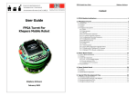
The Nios system showed in Figure 3.1 consists of three blocks:
1. Nios CPU
2. Peripheral Bus Module (PBM) – Avalon Bus
3. Set of peripherals
Detailed description of these blocks is mentioned in Nios documentation. Below
we deal with some important details of the Nios processor and the Avalon Bus.
3.1.1
Nios processor
Nios is a soft-core embedded processor from Altera, that includes a CPU optimized
for programmable logic and system-on-a-programmable chip (SOPC) integration
[3]. This configurable, general-purpose RISC processor can be combined with userdefined logic and programmed into an Altera PLD.
Chapter 3. Preliminaries: Software&Hardware Tools
8
Figure 3.1: Block diagram of the Nios system
The Nios CPU can be configured for a wide range of applications. Using the
SOPC Builder MegaWizard in Quartus software the parameters of the CPU, the
peripherals and the whole system module can configured for required solution.
The Nios family of soft core processors includes 32-bit and 16-bit architecture
variants. For more details about Nios CPU architecture, see Table 3.1 [3].
Table 3.1: Nios CPU architecture
Nios CPU details
Nios CPU
32-bit 16-bit
Data bus size (bits)
32
16
ALU width (bits)
32
16
Internal register width (bits)
32
16
Address bus size (bits)
33
17
Instruction size (bits)
16
16
3.1.2
Avalon Bus
An Avalon Bus included in the Nios is parameterized interface bus used for connecting on-chip processors (Nios) and peripherals into a SOPC. Avalon is an interface that specifies the port connections between master and slave components, and
specifies the timing by which these components communicate [6].
Apart from the simple wiring, the Avalon Bus module contains logic which
performs these major functions:
Chapter 3. Preliminaries: Software&Hardware Tools
9
1. Address-decoding to produce chip-select signals for each peripheral.
2. Data bus multiplexing to transfer data from a selecting peripheral to the master.
3. Wait-state generation to add extra clock-cycles to read- and write-accesses,
when required by the target peripheral.
4. Dynamic bus sizing to automatically execute multiple bus-cycles as required
to fetch (or store) wide data values from (to) narrow peripherals.
5. Interrupt Number Assignment to present the correct, prioritized IRQ number to the master when one or more peripherals is currently requesting an
interrupt.
The Avalon Bus offers a variety of options to tailor the bus-signals and timing
for different types of peripherals. In the case when wide master accessing a narrow
slave port two approaches are available:
Native address alignment A single transfer on the master port corresponds to
one transfer on the slave port, i.e. when a 32-bit master reads from a 16-bit
slave port, the Avalon Bus returns a 32-bit unit of data, but only the least
significant 16 bits contain valid data. The MSBs may be zero or undefined.
Dynamic bus sizing When a master reads from a slave port, while the master’s
wait-request input is asserted, the bus-logic executes so many read transfers
as required to fill the master data width.
3.2
SOPC Builder
SOPC Builder is used to construct embedded microprocessor systems that include
CPUs, memories, and I/O peripherals [10].
SOPC Builder consists of two substantially separate parts:
1. A graphical user interface (GUI) for listing and arranging system components.
Within the GUI, each component may also, itself, provide a graphical user
interface for its own configuration. The GUI creates a description of the system
called the system peripheral template file (PTF).
2. A generator-program that converts the system description (PTF file) into its
hardware implementation. The generator program (among other tasks) creates
an HDL (Hardware Description Language) description of the system and then
synthesizes it for the selected target device.
Chapter 3. Preliminaries: Software&Hardware Tools
10
In the first part we can add or remove the components of system, edit parameters of the Nios CPU, and the peripherals (e.g. value of registers number, base
address, IRQ nuber. . . ). All these settings can be done directly in any text editor
by editing the system PTF file.
In the second part following tasks are performed:
• Software files (header files, libraries) stored in project name sdk directory are
created.
• Every component’s individual generator program is run, for example, to create
an HDL description of the component. If no generator program is set, the
Default generator program performs simple copying HDL-files into the project
directory and arranging that component will be synthesized along with the
rest of the Nios SOPC module.
• The system-level HDL file is generated (in either VHDL or Verilog).
• The entire system module and all its component are synthesized using Altera
version of LeonardoSpectrum. The result is an EDIF1 -file ready for place-androute or as a module in a larger design.
When a new Nios system is going to be constructed the first step after the
Quartus project creating is running the SOPC Builder as Megawizard function [7].
In GUI we set parameters of the system.
The SOPC Buider generator program can be run in GUI or from the command line using a PERL script named generate project. The name of the project is
provided as a command-line argument.
3.3
Interfacing user-defined peripheral to SOPC
builder
When building a system using the SOPC Builder, modules from two sources can be
added:
1. Predefined modules delivered with SOPC builder, which are installed in the
SOPC Builder library (UART, timer, PIO. . . ).
2. User-defined modules.
All valid library components are recognized by the presence of a file named
class.ptf stored in component’s directory. This file declares and defines all the
information about that component: formal name of a component, a description of
1
An industry-standard format for the transmission of design data.
Chapter 3. Preliminaries: Software&Hardware Tools
11
its ports, a complete declaration of all I/O ports on the component, a description
of GUI for configuring the component etc (for more details see section 3.3.1).
A component’s library directory may also contain the logic that implement the
component, the software libraries, documentation and any other component-specific
information.
There are three broad mechanisms for using an SOPC Builder system module
with user-defined logic [10]:
Simple PIO connection: The PIO’s input- and output-pins will appear as I/O
ports at the top level module. After other logic is connected to these pins, the
system-module software can directly control logic level on each pin.
Instatiation inside the system module: A block of user-logic can be incorporated by instantiating it directly within the system module. SOPC Builder
will create bus-logic and connect it to all bus-ports on the user-designed block.
All I/O pins not designated as bus-connections will be promoted to the top
level, and appear as I/O pins on the system module.
Bus interface to external logic: SOPC Builder can add a set of bus-interface
pins customized to fit an external logic block. The bus interface includes
address, data, and control signals (including decoded device-select) suitable
for direct connection to a bus-interface on the device.
3.3.1
PTF File
SOPC Builder uses a system PTF file as a database to store information about an
SOPC System – master, sets of peripherals and Avalon Bus module. In principle,
to recreate a system module is possible by given only its system PTF file (and all
the necessary components in the library).
Each system PTF file contains a SYSTEM section with exactly one section
of type WIZARD SCRIPT ARGUMENTS and an arbitrary number of MODULE type sections [13].
WIZARD SCRIPT ARGUMENTS section describes global system-wide settings (like the system input clock frequency and the target device for synthesis).
The content of MODULE -type sections is initially taken from a module’s
definition in the library. A section of a module’s class.ptf file is copied into the
new MODULE section in the system’s PTF file.
Component’s PTF
Each component’s class.ptf file includes following parts [15]:
ASSOCIATED FILES: Describes programs which the SOPC Builder runs when
component is added (e.g. Java MegaWizard) in a SOPC system and a generator program’s name.
Chapter 3. Preliminaries: Software&Hardware Tools
12
DEFAULT GENERATOR: Sets a top-level module of the peripheral, and a selection, if user-defined logic should be synthesized along with the rest of the
system or will be incorporated as a black-box defined by EDIF-file can be done
in this part of PTF file.
USER INTERFACE: Specifies a text that will be shown up in SOPC builder’s
peripheral list.
MODULE DEFAULTS: Contains important facts about I/O ports, their names,
widths and directions, and parameters avalon role, that tell the SOPC Builder
how ports are to be connected to an Avalon bus. In addition gives a summary
information about connecting module (e.g. address alignment, number of wait
states. . . ).
The most important part of component’s PTF file is the MODULE DEFAULTS
part. In this part designer sets the parameters and signals of an interface between
the master and the slave and defines the conditions of a communication between
these two parts of SOPC system.
3.4
3.4.1
Software tools
Quartus
The Quartus II ver. 1.1 development software provides a complete design environment. The Quartus software offers a spectrum of logic design capabilities:
• Design entry using schematics, block diagrams, AHDL, VHDL, and Verilog
HDL
• Floorplan editing
• Powerful logic synthesis
• Functional and timing simulation
• Timing analysis
• Software source file importing, creation, and linking to produce programming
(configuration) files
• Combined compilation and software projects
• Automatic error location
• Device programming and verification
Chapter 3. Preliminaries: Software&Hardware Tools
13
During our work the Quartus software has been applicated for two important
tasks: a creation and a maintenance of the Nios system using the SOPC Builder
and the second operation is Place&Route, where a file for configuring Altera devices
and information about timing and area occupation have been obtained. For simulation and synthesis the ModelSim and LeonardoSpectrum software tools with better
features have been used.
3.4.2
ModelSim
As a simulation tool ModelSim PE ver. 5.5e has been chosen. This program is
widely used and in addition the Nios vendor Altera recommends ModelSim for Nios
simulation. Altera offers a good support for work with ModelSim: Altera devices’
description and simulation files for Library of Parameterized Modules (LPM) are
available for ModelSim.
Testbench
Testbenches have became the standard medthod to verify high-level language designs. Testbenches perform the following tasks:
• Instantiate the design under test (DUT)
• Stimulate the DUT by applying test vectors to the model
• Optionally compare actual results to expected results
Testbenches can be written in VHDL [11][28] or in Verilog. Since they are
used for simulation only, all behavioral constructs can be used. Testbenches can be
written more generically, making them easier to maintain.
For the DUT stimulating input values are needed. Since they are usually stored
in text file, a conversion from string to obtain std logic vector is needed. In addition the values can be stored in hexadecimal notation, when another conversion is
required [18].
After the output values are obtained, they can be compared to the expected
results. It is done by comparison the text files with actual and expected values.
Second method is the waveform comparison and the third commonly used method
is self-testing testbench [29].
3.4.3
LeonardoSpectrum
For synthesis the LeonardoSpectrum v2001.1 is used for the similar reasons as ModelSim for simulation. This tool is very popular and offers very powerful features for
synthesis.
The tool suite can be configured in three different levels of capability [24]:
Chapter 3. Preliminaries: Software&Hardware Tools
14
Level 1 produces the basic netlist. After input design files and technology are
selected, and optionally global timing constraints are set, a netlist is produced.
Special Altera version of the Level 1 is applied to crypted design files’ synthesis.
Level 2 adds more design capabilities (e.g. hierarchy preservation, advanced constraints etc.).
Level 3 supports scripts writing and running. Incremental optimization is possible,
what means, that a design is optimized at first, and a netlist is generated in
the next step, what is in contrast to Levels 1 and 2, where a netlist after each
optimization is created. In addition an Altera TimeCloser2 simulation flow is
supported.
3.4.4
GNUPro Software Development Tool
The software part of development is powered by GNUPro, a RedHat company. The
GNUPro Toolkit is an industry-standard open-source software development toolkit
optimized for the Nios embedded processor [36]. The toolkit includes a C/C++ compiler, macro-assembler, linker, simulator, debugger and numerous binary utilities,
and libraries.
Two programs from GNUPro have been utilized nios-build and nios-run. The
first one compiles, assembles, and links Nios source code. The output file with the
suffix .srec, is ready for downloading to the GERMS monitor running on the Nios
development board.
The nios-run downloads code to Nios development board and perform terminal
I/O.
3.5
Development board
During development and testing period a Nios development board [2] has been used.
The kit is provided by Altera together with software needed for development.
The board contains an APEX20K200EFC484-2X device, two 1 Mbit (64k × 16)
SRAM devices and one 8 Mbit (512k × 16) of flash memory device, RS-232 serial
port, JTAG connector and others components.
3.5.1
GERMS monitor
The GERMS monitor [4] is a simple monitor program that provides basic development facilities for the Nios development board. GERMS is a mnemonic for the
minimal command set of the monitor program included in the Nios development kit
(see Table 3.2).
2
The Altera TimeCloser flow is a two-pass synthesis flow where actual routing delays from a
first-pass place and route are used as the timing data for a second-pass optimization (see [23]).
Chapter 3. Preliminaries: Software&Hardware Tools
15
Table 3.2: GERMS monitor commands
Syntax
Description
G<base address>
Go (run a program)
E<base address>
Erase flash
R<base address>-<base address> Relocate next download
M<address>
Memory set and dump
S<S-record data>
Send S-records
:<I-hex record data>
Send I-Hex records
<CR>
Display the next 64 bytes of memory
<ESC>
Restart the monitor
3.5.2
APEX 20K200EFC484-2X device
Elementary device features are written in Table 3.3 [1]. A useful Nios system module
(CPU and peripherals) typically occupies between 25% and 35% of the logic on this
device.
Table 3.3: APEX20K200E device features
Maximum System Gates 525,824
LEs
8320
ESBs
52
Maximum RAM bits
106,496
Embedded System Block
To store a data in memory or for CPU registers implementation Embedded System
Blocks (ESBs) are used [5].
The ESB can implement various types of memory blocks, including dual-port
RAM, ROM etc. The ESB includes input and output registers. The input registers
synchronize writes, and the output registers can pipeline designs to improve system
performance. The ESB offers a dual-port mode, which supports simultaneous reads
and writes at two different clock frequencies (see Fig. 3.2).
When implementing memory, each ESB can be configured in one of the following
sizes: 128 × 16, 256 × 8, 512 × 4, 1024 × 2, or 2048 × 1. By combining multiple ESBs,
larger memory blocks can be implemented. Memory performance does not degrade
for memory block up to 2048 words deep.
The ESB implements two forms of dual-port memory: read/write clock mode
and input/output clock mode.
The read/write clock mode contains two clocks. One clock controls all registers
associated with writing: data input, WE, and write address. The other clock controls
Chapter 3. Preliminaries: Software&Hardware Tools
16
Figure 3.2: APEX 20K ESB Implementing Dual-Port RAM
all registers associated with reading: read enable (RE), read address, and data
output.
The input/output clock mode contains two clocks too. One clock controls all
registers for inputs into the ESB: data input, WE, RE, read address, and write
address. The other clock controls the ESB data output registers.
Chapter 4
Radix-2 Coprocessor
Implementation
In this chapter we describe the MM coprocessor implementation. We explain a
function of selected parts of the coprocessor and design considerations.
4.1
4.1.1
Design considerations
MM coprocessor
The main features of multiplier implemented in presented MM coprocessor are:
1. The ability to work on several operand precision.
2. The capability to be adjustable to PLD with different capacity.
3. A use a pipelined organization that reduces the impact on signal loads as a
result of high precision of the operands.
The ability to handle long-precision numbers with small precision operations
has been done using conventional multipliers, and a control algorithm that uses
these multipliers.
The second feature comes from the flexibility of the algorithm and hardware to
be adjusted in both word size and number of processing elements.
The high load on signals broadcast to several hardware components is an important factor to slow down high-precision Montgomery multiplier designs. For this
reason, the use of systolic structures have been considered by other researchers [12].
The organization of multiplier presented in this thesis is not purely systolic, and has
a flavour of serial-parallel implementation of the multiplication algorithm.
Structure of presented MM coprocessor is based on designs presented in [25]
and [19]. The coprocessor has been split in into two blocks: a multiplier block and
memory block (see Fig. 4.1).
Chapter 4. Radix-2 Coprocessor Implementation
18
Figure 4.1: Block diagram of MM coprocessor
A requirement to develop a pipelined version of the MM coprocessor has been
given during working. Design 1 described in section 4.2.1 is based on the version
presented in [19], the structure of basic MM unit is preserved. In Design 2 (section
4.2.1) the output pipeline registers of the MM unit are removed as well as the
registers between the stages to achieve lower area occupation.
4.1.2
Interface
Many decisions have been made during the development the interface between the
MM coprocessor and the Nios processor. In the next part interface-signals are
described, and the reasons for choosing their parameters are discussed.
The Figure 4.2 shows the signals used for communication between the MM
coprocessor and the Nios processor.
Figure 4.2: Block diagram of the interface between the MM coprocessor and the
Nios processor
Chapter 4. Radix-2 Coprocessor Implementation
19
Clock signal
In general, a peripheral connected to processor is wired to the same clock signal
as the processor. In our case, the MM coprocessor is able to run on higher clock
frequency as the master – Nios processor. Therefore we have used the possibility
to promote a signal of instantioned peripheral to the top level. It means that the
Nios system block has two separated input pins for clock signals: the first pin is
dedicated for the Nios processor’s clock, and the second one for the MM processor’s
clock.
Data signals
The width of input and output data signals are equal to the word width w in the
MM coprocessor. Thanks to dynamic address alignment (see section 4.1.3) from the
Nios’ point of view is the data width equal to the inner data bus, i.e. 16 bits for
the 16-bit Nios and 32 bits for the 32-bit Nios. The value of data width is the only
interface parameter that is different for Nios 16- and 32-bit.
Address signal
The way how are data in the coprocessor mapped in its memory is described in part
4.4. The width of address signal varies in dependency on the version of implemented
coprocessor, according to the number of words e.
Other signals
Three additional signals are used in the interface:
Reset signal is provided for all peripherals of the Nios system.
Chip select signal is used by the write process. Input data are stored only when
chip select signal is activ.
Write enable signal is in combination with the chip select signal used to control
the correct data storing to the memory. The signal indicates that the current
bus transaction ia a write-data operation.
4.1.3
Address alignment
In section 3.1.2 two different modes of the address alignment are described. The
dynamic alignment has been chosen. Below are two main reasons for dynamic
alignment selection:
• it enables the Nios to perform data transfers as if the coprocessor have been
always the same width as the processor.
Chapter 4. Radix-2 Coprocessor Implementation
20
• it simplifies software design for the Nios, by eliminating the need for software
to splice together data from the coprocessor.
There is no way for the 32-bit wide processor to read from only 16-bit location
in the coprocessor, but this disadvantage of dynamic memory alignment is not important in our case. All operations in the processor are computed with full data
width.
4.2
Multiplier block
The crucial block of the MM coprocessor is a multiplier block which is based on the
version presented in [19], a unit realizing inner part of the main loop in Algorithm
2.2. Block provides control for basic MM units, and manages a data exchange with
a memory block.
To fulfil these aims, the block contains logic for:
• generating read and write addresses and write enable signal for memories
• counting number of the cycles, the words and the bits in the word
• generating all other supporting signals for basic multiplication unit
A word width w, number of words e, and number of stages n are values, that can
be set as a parameter with arbitrary value with limitations given by target device
and/or by chosen control structure of the coprocessor.
In order to reduce storage and arithmetic hardware complexity, data path of
MM coprocessor uses X, Y and M in a standard non-redundant form. The internal
sum S is received and generated in the redundant Carry-Save form [31]. Therefore
the bit resolution of the sum S is effectively doubled.
Each MM unit propagates the words Y and M and the newly computed words
of 1 S and 2 S to the next MM unit, which performs another computational loop of
the MM algorithm and on its turn propagates the words of Y and M and the newly
computed words of 1 S and 2 S, with a latency of 3 cycles (Design 1) or 2 cycles
(Design 2).
The first stage gets data from memory and the results propagates to the next
stage, the last stage stores data to the memory. When only one stage is implemented,
data are directly stored to the memory.
In the next part two similar design are presented. In Design 1 the MM unit
design from the previous implementation [19] is preserved. In Design 2 we have
removed the output pipeline register, and afterwards also the registers between the
stages. Comparison of both solutions is presented in section 6.
Chapter 4. Radix-2 Coprocessor Implementation
4.2.1
21
Design 1
The data path is organized as a pipeline of MM units (see detailed description in
section 4.2.4) separated by registers (Fig. 4.3). A stage consists of a MM unit and a
register. The MM unit implements one iteration of the inner loop in the MWR2MM
algorithm (Algorithm 2.2 in section 2.3). Each stage gets as inputs one word of Y ,
M , 1 S and 2 S each clock cycle. Depending on the computations progress, one bit
of X is loaded in a different stage every 3 clock cycles.
Figure 4.3: Block diagram of multiplier data path
4.2.2
Design 2
The output pipeline registers in the MM unit and the registers between the stages
have been removed in this version. The results are directly propagated to the next
stage or are stored to the memory in case with one stage.
The motivation for developing of this version is in a possibility to obtain the
design with lower area occupation.
4.2.3
Parallel computation
In previous work [19] the only one MM unit was used, our aim was to implement
solution, where the parallelism of algorithm is utilized. Short analysis of data dependencies [39] shows that the degree of pipelining and parallelism can be very
high.
The dependency between operations within the loop for j restricts their parallel
execution due to dependency on the carry – c. However, parallelism is possible
among instructions in different i loops. Results from one MM unit are not stored in
the memory, but may be passed to the next MM unit.
The maximum degree of pipeline that can be attained with this organization is
found as
Chapter 4. Radix-2 Coprocessor Implementation
(
e
=
x
pmax
x=
22
3 for Design 1
2 for Design 2
(4.1)
To preserve not too much complicated control structure of coprocessor, use of
n, where n | e (i.e. for e = 32, n ∈ {1, 2, 4 . . .}), stages is only possible. The second
limitation is the width of word w, in presented version of the coprocessor n ≤ w has
to be fulfilled. When less than pmax stages are available, the total execution time
will increase, but it is still possible to perform the full precision computation with
smaller circuit.
The total computation time T (in clock cycles) when n ≤ pmax modules (stages)
are used in the pipeline is
k2
we
+ xn =
+ xn
T =e
n
wn
4.2.4
(
x=
3 for Design 1
2 for Design 2
(4.2)
MM unit
The design of data path is based on the structure presented in [39]. MM unit consists
of two layers of carry-save adders and it is shown for w = 3 in Fig. 4.4.
!
" #$% &' #" &
Figure 4.4: Structure of MM unit for w = 3 (FA – Full Adder)
Input c represents latched value t(0) that is the least significant bit of the value
(0)
S (0) + xi Y (0) (c = t(0) = S0 ). This value is computed at the beginning of the main
loop (when j = 0).
Chapter 4. Radix-2 Coprocessor Implementation
23
While computing the word j (step j in the internal loop in algorithm 2.2, the
circuit generates 2(w − 1) bits of S (j) , and two most significant bits of S (j−1) . The
bits of S (j−1) computed at step (j − 1) must be delayed and concatenated with the
most significant bits generated at step j. In Design 1 output data are stored in the
output pipeline register.
The problem with S-value reset (step 1 in Algorithm 2.2) was solved in the
previous version of the coprocessor [19], the reset signal to the input pipeline register
is used (see Fig. 4.4).
Two output signals have been added – the registered values of the operands
Y and M are connected to the next stage’s register in Design 1 (see Fig. 4.3) or
directly to the next stage. The reason why the structure is solved in this way is a
delay between the moment when actual input values are present on the input and
the moment when the results appear on the output of MM unit.
In the first clock cycle data are stored to the input pipeline registers. In the
second cycle they are propagated to the adders, and afterwards thy are presented
on the output of the MM unit in Design 2 or are delayed during the next clock cycle
in the output pipeline registers in Design 1. Thus, together three clock cycles delay
in Design 1, and two clock cycles delay in Design 2 is between the stages, in which
the same values of Y and M operands are used for computing.
4.2.5
State machine
To control the multiplier’s function the state machine with 4 states (wait, prepare,
run, finished) is used.
The initial state is the wait state. In this state the block is ready for new
processing. Loading or storing data to memories is possible.
After the input signal start is set, the state is changed to prepare state. All
needed input signals of MM unit are initialized, also counters’ values are set to zero.
After one clock cycle the state run follows.
During this state the computation process is running. The access from the Nios
processor to the memories with results 1 S and 2 S is forbidden.
After the value of cycle counter reaches the expected value the state is changed
to finished and after one clock cycle back to the initial state wait. Afterwards next
process can start.
4.2.6
Memory control signals
In the multiplier block all needed signals to store data to the memory and to load
data from the memory are generated.
Chapter 4. Radix-2 Coprocessor Implementation
24
Data storing process
All input operands (X, Y , and M ) have to be stored in memory before the multiplication process starts. Multipliers modifies only a content of 1 S and 2 S memories,
where the intermediate values and final values of results are storing.
Write enable signal of S memories is active during the run state of the state
machine. Although the output values from the last stage are not valid from the
beginning, they are stored and afterwards overwritten by valid values after a write
address is initialized.
The write address of S memories is derived from the word counter. When the
first valid values of S operands appear on the output of the last stage, the write
address is initialized.
Data reading process
During multiplication or squaring operation the operands X, Y , M and S have to
be read from the memory in different order.
Intermediate results stored in S memories, and operands Y and M are read
every clock cycle, the read address is equal to the value of the word counter.
The multiplier X value is changed in a different order. The word of X is loaded
from the memory X or Y and temporary stored in a shift register. If the squaring
flag is set, the word from Y memory is read. Once the precision is exhausted,
another word of X is taken. The number of cycles between two read operations
depends on the number of stages and the width of word.
4.2.7
Counters
System of three counters control the computation process: a cycle, a word, and a
bit counter. Values all of them are initialized by start signal. In addition the value
of the word counter is set to zero, when new bit of X word is scanned, and the bit
counter is initialized after the next X word is stored in the shift register.
4.3
Memory block
The most important parameter influencing the overall multiplier speed is the memory access time.
Since during one cycle current result from the last stage has to be written
and previous result has to be read to the first stage from the same memory, we
have chosen to configure the memory block as a dual port RAM. An Altera-specific
function lpm ram dp() from the LPM is used. List of variables, which have to be
store consists of:
• X – input value, multiplier
Chapter 4. Radix-2 Coprocessor Implementation
25
• Y – input value, multiplicand
• M – input value, modulus
• 1 S and 2 S – input/output value, intermediate and final result
Thus we operate together with five memory blocks, which are implemented in
ESBs of APEX device (see details in section 3.5.2). In previous solution the sixth
memory block was used as a work memory because of lack of the memory in the
PIC processor.
The memory block is shared by both the Nios processor and the MM coprocessor. Therefore special attention has been paid to connection of this block in correct
way. It means, that the lpm ram dp() function’s parameters are set to be suitable
as for the processor as well as for the coprocessor.
To achieve this goal the following procedure has been applied.
1. Vendor-defined on-chip RAM has been connected as a peripheral to the Nios
processor.
2. After the project has been generated, the PTF and the Verilog1 file of connected memory have been obtained. Verilog file describes the memory as the
lpm ram dp() function, the PTF provides information about the interface to
Nios.
3. For functional verification of implemented memory a very simple code for
reading and writing to memory have been written in C language.
4. The parameters from the PTF and from the Verilog file have been utilized to
create new similar files (in VHDL) with parameters of our peripheral (different
size of memory. . . ).
5. A new user-defined peripheral has been used following the procedure mentioned in SOPC Cookbook [15] by using the files generated in the previous
steps.
6. After new project generation and compilation and after device programming
the simple code to test connected peripheral have been run.
We consider this method as very useful and quite quick way how to find out
correct connection parameters of the user-defined peripherals, which are similar to
the vendor-defined peripherals.
After applying the procedure mentioned above the following parameters for
lpm ram dp() function have been set in the memory block of the MM coprocessor:
1
Although the VHDL has been selected for our project all output files are in Verilog, only files
for simulation are translated to VHDL by SOPC Builder.
Chapter 4. Radix-2 Coprocessor Implementation
LPM_INDATA
LPM_WRADDRESS_CONTROL
LPM_RDADDRESS_CONTROL
LPM_OUTDATA
=>
=>
=>
=>
26
"REGISTERED",
"REGISTERED",
"UNREGISTERED",
"UNREGISTERED"
Output data for reading are available immediately after receiving the read address therefore no additional wait state for the Nios processor is needed. Input
data and write address are registered what assures error-free synchronized writing
process.
4.4
Interface block
The third part of coprocessor represents the interface between the Nios processor
and the MM coprocessor. The block is very simple thanks to features of the Avalon
Bus.
Input address is already decoded by the Avalon Bus (see section 3.1.2), therefore only elementary mapping operation is required. First 3 bits of address signal
indicates the memory block implemented in EMB, the remaining bits are equal to
the address used within the coprocessor and represents the address of words in the
coprocessor’s memory.
Write enable and chip select signals control the writing process to the memory
block of the coprocessor. After the address decoding, chip select signal of the coprocessor is asserted and write enable signal is active to indicate the write operation to
the memory. Afterwards data from the processor presented on the write data input
are valid, and can be stored to the coprocessor’s memory according to the write
address.
The reading process is much more easily. Data available on the read data output
are read by the Nios processor only in that case when the read address of the MM
coprocessor is valid. Then the Avalon Bus connects the coprocessor’s data output
to the Nios processor’s data input using the Data in multiplexer (see picture 3.1).
Write enable signal for specific memory block is generated as a logical AND of
input write enable signal and chip select signal and of the memory block’s address.
During the development process all memory blocks have been accessible as for
reading as well as for writing. This is not necessary in the final version, where the
processor is able to write to X, Y and M memory and can read from the memories
1 S and 2 S.
To control the coprocessor and to check its status two registers are implemented
in the coprocessor as a part of the interface. The length of registers is the same as
the input and output data width.
The first register is called control register and aims for sending simple commands
to the coprocessor. In presented version only two LSB bits of register are used with
next functions:
Chapter 4. Radix-2 Coprocessor Implementation
27
0. bit controlling the multiplication/squaring process (set 1 to run computation)
1. bit switching between the multiplication and squaring (set 0 to multiply input
values, set 1 to square value stored in memory Y )
When other address than address of 1 S or 2 S memory is on the input of coprocessor the content of the second status register is presented on the data output.
Only one bit (LSB) is used for the coprocessor status indication in this register.
When the coprocessor is running (states prepare or run) the value of the 0.bit is 1,
else 0.
4.5
Testing software
After the synthesis, the Place&Route procedure, and the programming the target
device, a correct function of the system has been tested.
For simple reading from and writing to the coprocessor’s memory the commands
of the GERMS monitor have been utilized. To verify the results of the multiply
operation, simple programs in C have been written. In the last step we have applied
the MM coprocessor to RSA. Short description of RSA code is mentioned in the last
part of this section.
Simple program for the coprocessor testing executes the following procedures:
1. Starts the timer.
2. Writes data to X, Y , and M memories.
3. Changes the contents of the control register – starts the multiplication process.
4. Checks the status register and waits for the results.
5. Stops the timer.
6. Prints the results from the MM coprocessor, and the value of time taken for
writing to the memories, and for multiplication.
For the operations with timer a function nr timer milliseconds() is used. Writing to the control register is solved using a function in assembler:
MOVI
ST
NOP
MOVI
ST
NOP
%g0,1
[%i4],%g0
;Value for the MM control register
;Write MM control register
%g0,0
[%i4],%g0
;Value for control register
;Write MM control register
Similarly for reading from the status register a function in assembler is used:
Chapter 4. Radix-2 Coprocessor Implementation
TEST:
LD
%g0,[%i4]
SKP0
%g0, 0
BR TEST
NOP
4.5.1
28
;Test the MM status register
;Load status
;Check if zero
;If not, jump to TEST
RSA
For testing of the MM coprocessor and for obtaining the timing results of application the coprocessor to RSA the code realising the Montgomery multiplication
(Algorithm 2.1) has been used. Code is prepared for 16-bit version of Nios, and
executes the RSA algorithm with k = 1024-bits operands.
Precomputed input values R2 mod M and R mod M are stored in the Nios’s
memory, and are not computed. The encryption time is obtained for the F4 exponent. For decryption we apply the 1024-bit exponent including 528 ones, i.e.
the multiplication process is executed 528 times (step 6 in Algorithm 2.1), and the
squaring process 1024 times (step 4 in Algorithm 2.1).
Chapter 5
Methodology
In this chapter we describe a work made during the development and testing MM
coprocessor and its connection to the NIOS processor.
5.1
Code translation
Since all source files of previous coprocessor’s implementation have been written in
AHDL, the first aim has been the translation to VHDL or to Verilog language.
Both the simulation tool ModelSim and the synthesis tool LeonardoSpectrum
[22] are not able to work with AHDL, programs support only designs described by
VHDL or Verilog language. Because we have had some experiences with VHDL
during working on other projects and the ModelSim license has been available for
VHDL only, the VHDL has been selected as a language for design description.
5.2
Simulation
The simulation has been necessary as during the translation the source code to
VHDL as well as later during the interface and control software development.
Very useful feature is a possibility to simulate the system as a whole, i.e. MM
coprocessor connected to the Nios processor with the executable code stored in onchip memory and simulated input of UART [9].
Since the system is embedded in PLD, sometimes the simulation has been the
only possibility of how to verify correct function of system or to find sources of
errors.
In comparasion to the simulation process using Altera MaxPlus II development
tool, in ModelSim all design signals’ names stay preserved and can be easily added
to the list of simulated signals.
Next part describes three ways how the input signals can be stimulated:
• For simple designs with small amount of signals the GUI can be used to
force/unforced signals’ values. All steps in GUI are translated to commands,
Chapter 5. Methodology
30
which are executed in command line. ModelSim commands written in text file
form so called “do” file [35].
• Very often a need for using the same settings and/or values of input signals
is actual. In “do” file all of ModelSim commands [34] can be stored and used
for different projects.
• To make the simulation process even more comfortable a self-testing testbench
– one that automates the comparison of actual to expected testbench results,
can be applied. For more details see section 3.4.2 or [29], [18].
All these method can be combined to achieve a required behavior of input or
internal signals of design.
Many times used feature of ModelSim simulator is a possibility to divide signals
in several groups or to change a wave color. When the multiplier block was simulated,
we needed to check both the I/O signals of the module and the internal and MM
unit’s signals. If all signals are situated in one window, checking is difficult and
is getting long-winded. To keep all signals ordered, one group of signals has been
added in the wave window, afterwards new window pane has been open and the
second group of signals has been added. It is a very good way how to keep a bunch
of signals sorted and readable.
5.2.1
The MM coprocessor simulation
In the first period of the development, when particular blocks of the coprocessor
has been translated to VHDL, mainly “do” files has been applied to set the initial
values of input signals.
For testing the MM unit and also the multiplier block test vectors from previous
project has been utilized. The results has been checked in the waveform window of
simulator. After the connection of the memory block to the multiplier block, the
MM coprocessor has been tested using the self-checking testbench.
The input file containing the hexadecimal values of input operands X, Y , and
M , and the expected values of result 1 S and 2 S, have been read by testbench. Also
clock signal, start signal and signals controlling the write process to the memory
have been generated by testbench. Afterwards, during the results storing in the
memory, the values have been compared to the results written in the input file. If
the values have not been the same a error message set in testbench has been quoted
to the command line of the simulator.
After the features and design of the interface block has been stated, we have
written another testbench file to simulate the communication between the processor
and the coprocessor. In this way all output signals of the Nios processor have been
generated by testbench. Also the output values have not been checked during their
storing in the memory, but the read process from the processor’s memory has been
simulated and values obtained from the coprocessor have been compared with correct
values.
Chapter 5. Methodology
5.2.2
31
The Nios processor simulation
Before a design has been downloaded to the development board, the simulation has
been executed to verify correct function of the block. Since the simulation without
running program code is not useful, problem how to simulate an executable code
had to be solved.
The easiest way is to store the code in the on-chip memory and run it with
GERMS monitor’s commands. But there is a bug in how Nios ver. 1.1.1 reads srec
files and stores them in internal memory. Basically, the vector table is not taken into
account and the first 64 words of the srec file are not overwritten by the vector table.
We have received1 a PERL script srec2mif that converts a SREC file into a MIF file
and pads the first 64 locations of the mif file with 0’s. During the VHDL simulation
files generation process mif files are converted to dat files, and the content of all
memories is initialized from dat directly in VHDL code.
After this correction the executable code in the on-chip memory works properly
and can be started by Gxxxx command in GERMS monitor shell (xxxx have to be
rewritten by a start address of the main program memory, in which the code is
stored).
UART input simulation
A method how the monitor’s command can be simulated is quite simple. Below is
showed an example of character stream.dat file stored in project name sim directory.
@0000
0A 47 31 30 30 30 0A 0D
00
In simulation, the Nios UART will read this file as a source of simulated
character-input. This example “types” the string:
<LF> G1000 <CR>
Which is a command to the monitor telling it to start executing code at address
1000. Changes of the file have to be done before the simulation files are generated.
Simulation flow
In the next part a simulation flow is shortly described [16]. We suppose that the
Nios system project is created, the MM coprocessor is connected, and a source file
with program is written.
1. Use nios-build script to generate executable code.
1
This bug has been fixed by Altera applications engineer via mySupport system [14].
Chapter 5. Methodology
32
2. Use srec2mif script to convert obtained srec file into a mif file.
3. In the System Builder menu create a new on-chip ROM memory and set the
generated mif file as a content. In the next Builder’s window select newcreated on-chip memory as the main program and data memory, and in the
third window specify interrupt vector table location in on-chip memory. Finally generate the project and close the Quartus II.
4. Repeat steps 1 and 2 to generate the code with new libraries and header files.
5. Edit the character stream.dat file if it is necessary.
6. Use generate project script to generate the project.
7. Make a correction (add “.txt”) in the project name test bench.v file at the line,
where the name of the user-defined peripheral top entity’s name is mentioned
to
‘include "../top_entity_name.vbb.txt"
and save it.
8. Run vhdl simulation script to generate the simulation files in the directory
project name sim.
After this procedure VHDL simulation files are created and ready to be used
in the simulation tool.
5.3
Synthesis
In many cases the LeonardoSpectrum synthesis tool has been applied.
Basically LeonardoSpectrum is used for synthesis of the Nios system by System
Builder. The source code of the Nios processor is encrypted, therefore Altera version
of LeonardoSpectrum Level 1 is required.
The best way of how to implement the MM coprocessor is to synthesize it
along with the Nios system what is due to problem with a license2 impossible.
Therefore the coprocessor is connected as a black box component, what means that
the peripheral is synthesized as a separated block and afterwards it is implemented
in the Nios system.
Mostly the Level 2 has been used for synthesis of the MM coprocessor. The
input design files have been selected, and the top level design has been marked.
Afterwards the following optimization settings have been set:
2
The Nios source code is written in Verilog, MM coprocessor is described by VHDL. Problem
with VHDL/Verilog license is fixed only in version Nios 2.0.
Chapter 5. Methodology
33
• Extended optimization effort: pass 1-4
• Optimize for: Auto
• Hierarchy: Auto
• Add I/O pads: Disabled
The last item is very important. The I/O pads must not to be added, since the
coprocessor is later connected to the Nios processor, and is incorporated in the Nios
top-level design.
After the synthesis flow is done, the EDIF-file (.edf ) is generated, and ready for
using in the next procedure (for place-and-route or as a module in a larger design).
The results presented in chapter 6 have been obtained after a Place&Route (P&R)
process in Quartus II development tool.
If the obtained maximal clock frequency is not sufficient, a procedure described
in [21] can be followed. In this case, the required clock frequency is given, and the
LeonardoSpectrum tries to reach this value.
Chapter 6
Results and comparisons
Presented implementation results are generated after the synthesis in LeonardoSpectrum v2001.1 and following Place&Route procedure in Altera Quartus II, ver. 1.1
development system. Area occupation expressed in Logic Elements (LEs) and maximal possible PLD clock frequency (fclk ) for Altera PLD APEX 20K200EFC484-2X
are given in tables for several versions of the MM coprocessor and for selected combinations of the coprocessor’s parameters: word width w, number of words e, and
number of stages n. In addition tables with comparison of implemented versions are
presented.
6.1
Design 1
In Tables 6.1-6.3 we show the results of Design 1 mapping. Description of Design 1
is given in section 4.2.1.
Table 6.1: Design 1 – Area occupation (LEs)/max fclk (MHz) of the MM coprocessor
(k = 1024 bits)
n=1
n=2
n=4
n=8
w=8
w = 16
w = 32
LEs fclk
LEs
fclk
LEs
fclk
281 69.98 429 70.01 776 67.14
439 65.73 743 69.01 1394 62.56
757 62.8 1365 70.69 2618 67.2
N/A
2609 65.63 5125 66.35
Chapter 6. Results and comparisons
35
Table 6.2: Design 1 – Area occupation (LEs)/max fclk (MHz) of the MM coprocessor
(k = 2048 bits)
n=1
n=2
n=4
n=8
w=8
w = 16
w = 32
LEs fclk
LEs
fclk
LEs
fclk
292 70.18 446 55.91 786 62.24
446 65.93 752 64.64 1404 67.08
765 52.44 1378 56.31 2635 57.52
N/A
2619 65.45 5137 64.57
Table 6.3: Design 1 – Area occupation (LEs)/max fclk (MHz) of the MM coprocessor
(k = 4096 bits)
n=1
n=2
n=4
n=8
w=8
w = 16
w = 32
LEs fclk
LEs
fclk
LEs
fclk
302 68.32 455 61.64 832 59.44
461 64.3 763 63.61 1413 54.92
779 63.51 1386 65.41 2695 60.61
N/A
2632 61.49 5151 60.41
Chapter 6. Results and comparisons
6.2
36
Design 1a
To make possible the comparison of two types of coprocessor structure, we have
changed the coprocessor design. In following design named Design 1a, the coprocessor is not split in two parts (the multiplier block, and the memory block), but
in three parts (multiplier, memory, and interface block), where the interface logic is
removed from the top-level design to the new-created interface block. This structure is recommended in Advanced synthesis training [21] to obtain better results of
mapping.
Table 6.4: Design 1a – Area occupation (LEs)/max fclk (MHz) of the MM coprocessor (k = 1024 bits)
n=1
n=2
n=4
n=8
w=8
w = 16
w = 32
LEs fclk
LEs
fclk
LEs
fclk
273 69.37 413 63.28 744 62.24
429 64.11 727 62.24 1362 70.09
749 65.58 1349 71.51 2586 67.64
N/A
2593 64.89 5093 63.19
Table 6.5: Design 1a – Area occupation (LEs)/max fclk (MHz) of the MM coprocessor (k = 2048 bits)
n=1
n=2
n=4
n=8
w=8
w = 16
w = 32
LEs fclk
LEs
fclk
LEs
fclk
284 64.6 430 63.12 754 61.93
438 64.48 736 62.05 1372 67.53
757 65.57 1362 71.8 2603 49.84
N/A
2603 65.86 5105 65.16
Table 6.6: Design 1a – Area occupation (LEs)/max fclk (MHz) of the MM coprocessor (k = 4096 bits)
n=1
n=2
n=4
n=8
w=8
w = 16
w = 32
LEs fclk
LEs
fclk
LEs
fclk
294 66.31 439 62.91 803 59.1
453 62.17 747 63.55 1381 61.65
771 65.81 1370 64.5 2663 60.76
N/A
2616 64.04 5119 60.46
Chapter 6. Results and comparisons
6.3
37
Comparison of Design 1 and Design 1a
In the following tables (6.7-6.9) we compare the results of mapping for Design 1
and for Design 1a. While differences in area occupation are small, and are not
presented in tables, the values of maximal clock frequency are significantly different
for some combinations of the coprocessor’s parameters. The difference of maximal
clock frequency for Design 1a and for Design 1 is expressed as
∆fclk = fclk1a − fclk1
(6.1)
Table 6.7: Comparison of max fclk (MHz) for Design 1 and Design 1a (k = 1024
bits)
n=1
n=2
n=4
n=8
w = 8 w = 16 w = 32
∆fclk
∆fclk
∆fclk
-0.61
-6.73
-5.0
-1.62
-6.77
+7.53
-2.78 +0.82
+0.44
N/A
-0.74
-3.16
Table 6.8: Comparison of max fclk (MHz) for Design 1 and Design 1a (k = 2048
bits)
n=1
n=2
n=4
n=8
w = 8 w = 16 w = 32
∆fclk
∆fclk
∆fclk
-5.58
+7.21
-0.31
-1.47
-2.59
+0.45
+13.13 +15.49 -7.68
N/A
+0.41
+0.59
Table 6.9: Comparison of max fclk (MHz) for Design 1 and Design 1a (k = 4096
bits)
n=1
n=2
n=4
n=8
w = 8 w = 16 w = 32
∆fclk
∆fclk
∆fclk
-2.01 +1.27
-0.34
-2.13
-0.06
+6.73
+2.3
-0.91
+0.15
N/A
+2.55
+0.05
The most important difference of clock frequency has been obtained for k =
2048, where for n = 4 and w = 16 the maximal frequency of Design 1a is 65.57
MHz, and frequency of Design 1 is 52.44 MHz.
Chapter 6. Results and comparisons
38
We can say that for some combinations of coprocessor parameters better results
have been reached when the coprocessor is split in three blocks. On the other
hand for other combinations the clock frequency is lower. It means that optimal
coprocessor organisation depends on chosen parameters.
6.4
Design 2
In Tables 6.10-6.12 the results of Design 2 mapping are presented. Description of
Design 2 is given in section 4.2.2.
Table 6.10: Design 2 – Area occupation (LEs)/max fclk (MHz) of the MM coprocessor (k = 1024 bits)
n=1
n=2
n=4
n=8
w=8
w = 16
w = 32
LEs fclk
LEs
fclk
LEs
fclk
264 71.28 396 62.74 711 68.46
387 60.95 643 71.49 1196 61.73
637 71.05 1139 60.86 2168 61.68
N/A
2123 61.26 4113 61.45
Table 6.11: Design 2 – Area occupation (LEs)/max fclk (MHz) of the MM coprocessor (k = 2048 bits)
n=1
n=2
n=4
n=8
w=8
w = 16
w = 32
LEs fclk
LEs
fclk
LEs
fclk
274 62.57 413 64.48 721 63.03
396 62.29 655 62.88 1208 61.52
648 70.81 1142 71.73 2180 61.80
N/A
2135 71.55 4125 59.41
Table 6.12: Design 2 – Area occupation (LEs)/max fclk (MHz) of the MM coprocessor (k = 4096 bits)
n=1
n=2
n=4
n=8
w=8
w = 16
w = 32
LEs fclk
LEs
fclk
LEs
fclk
284 69.34 422 61.82 770 57.48
408 63.33 666 62.07 1159 63.35
663 65.83 1159 63.35 2186 61.84
N/A
2145 67.51 4138 60.45
Chapter 6. Results and comparisons
6.5
39
Design 2a
From the same reason as for creation Design 1a we have prepared Design 2a, and in
Tables 6.13-6.15 we present the results of area occupation and maximal fclk of the
MM coprocessor.
Table 6.13: Design 2a – Area occupation (LEs)/max fclk (MHz) of the MM coprocessor (k = 1024 bits)
n=1
n=2
n=4
n=8
w=8
w = 16
w = 32
LEs fclk
LEs
fclk
LEs
fclk
256 57.24 380 61.75 679 62.67
379 60.35 627 64.77 1164 62.74
629 67.59 1123 71.01 2136 58.18
N/A
2107 69.95 4081 64.55
Table 6.14: Design 2a – Area occupation (LEs)/max fclk (MHz) of the MM coprocessor (k = 2048 bits)
n=1
n=2
n=4
n=8
w=8
w = 16
w = 32
LEs fclk
LEs
fclk
LEs
fclk
266 55.22 397 66.49 689 62.38
388 64.56 639 55.07 1176 61.68
640 64.61 1126 70.16 2148 61.36
N/A
2119 62.03 4093 66.62
Table 6.15: Design 2a – Area occupation (LEs)/max fclk (MHz) of the MM coprocessor (k = 4096 bits)
n=1
n=2
n=4
n=8
6.6
w=8
w = 16
w = 32
LEs fclk
LEs
fclk
LEs
fclk
276 68.99 406 66.46 738 54.58
400 63.08 650 63.46 1190 62.85
655 62.63 1143 64.23 2154 58.93
N/A
2129 64.22 4106 63.72
Comparison of Design 2 and Design 2a
In this subsection we compare the clock frequency for Design 2 and for Design 2a
(Tables 6.16-6.18 ). Like for comparison of Design 1 and Design 1a only differences of
Chapter 6. Results and comparisons
40
clock frequency are showed, since the results of area occupation are similar for both
designs. The difference of maximal clock frequency for Design 2a and for Design 2
is expressed as
∆fclk = fclk2a − fclk2
(6.2)
Table 6.16: Comparison of max fclk (MHz) for Design 2 and Design 2a (k = 1024
bits)
n=1
n=2
n=4
n=8
w = 8 w = 16 w = 32
∆fclk
∆fclk
∆fclk
-14.04 -0.99
-5.79
-0.6
-6.72
+1.01
-3.46 +10.15
-3.5
N/A
+8.69
+3.1
Table 6.17: Comparison of max fclk (MHz) for Design 2 and Design 2a (k = 2048
bits)
n=1
n=2
n=4
n=8
w = 8 w = 16 w = 32
∆fclk
∆fclk
∆fclk
-7.35 +2.01
-0.65
+2.27 -7.81
+0.16
-6.2
-1.57
-0.44
N/A
-9.52
+7.21
Table 6.18: Comparison of max fclk (MHz) for Design 2 and Design 2a (k = 4096
bits)
n=1
n=2
n=4
n=8
w = 8 w = 16 w = 32
∆fclk
∆fclk
∆fclk
-0.35 +4.64
-2.9
-0.25 +1.39
-3.64
-3.2
+0.88
-2.91
N/A
-3.29
+3.27
Likewise for the comparison of Designs 1 and 1a, for the comparison of Design 2
and Design 2a we can say that splitting the coprocessor in three parts, and removing
logic from the top-design module does not automatically bring better results of
maximal clock frequency, and this rule is not valid in general.
Chapter 6. Results and comparisons
6.7
41
Comparison of Design 1 and Design 2
In Tables 6.19-6.21 an impact of removing the output pipeline register and the register between the stages in Design 2 is presented. The difference between the maximal
clock frequencies is not so significant, but we can say that Design 2 reaches lower
frequencies than Design 1, what has been expected (see [19], where by adding the
pipeline registers in MM unit better results for clock frequency have been obtained.)
An advantage of Design 2 is lower area occupation. For example for w = 32 and
n = 8 more than 1000 LEs can be saved in the target device. The differences of
maximal clock frequency and area occupation for Design 1a and for Design 1 are
expressed as
∆fclk = fclk2 − fclk1
∆LEs = LEs2 − LEs1
(6.3)
Table 6.19: Comparison of area occupation (LEs)/max fclk (MHz) for Design 1 and
Design 2 (k = 1024 bits)
n=1
n=2
n=4
n=8
w=8
w = 16
w = 32
∆ LEs ∆fclk ∆ LEs ∆fclk ∆ LEs ∆fclk
-17
+1.3
-33
-7.27
-62
-1.32
-50
-4.78
-100
+2.48
-198
-0.83
-120
+8.25
-226
-9.83
-450
-5.52
N/A
-486
-4.37 -1012 -4.87
Table 6.20: Comparison of area occupation (LEs)/max fclk (MHz) for Design 1 and
Design 2 (k = 2048 bits)
n=1
n=2
n=4
n=8
6.8
w=8
w = 16
w = 32
∆ LEs ∆fclk ∆ LEs ∆fclk ∆ LEs ∆fclk
-18
-10.57
-33
+8.57
-65
+0.79
-50
-3.66
-97
-1.76
-196
-5.56
-117
+18.37
-236
+15.42
-455
+4.28
N/A
-484
+6.1
-1012 -5.16
Computation time
The total computation time of MM operation TM M (according to the equation 4.2)
is:
(
1 k2
3 for Design 1
TM M =
+ xn
x=
(6.4)
2 for Design 2
fclk wn
Chapter 6. Results and comparisons
42
Table 6.21: Comparison of area occupation (LEs)/max fclk (MHz) for Design 1 and
Design 2 (k = 4096 bits)
n=1
n=2
n=4
n=8
w=8
w = 16
w = 32
∆ LEs ∆fclk ∆ LEs ∆fclk ∆ LEs ∆fclk
-18
+1.02
-33
+0.18
-65
-1.96
-53
-0.97
-97
-1.54
-191
+11.77
-116
+2.32
-227
-2.06
-509
-1.23
N/A
-487
-6.02 -1013
+0.04
Performance of implemented MM coprocessor for word length w = 32 and for
Design 1 (x = 3 in equation 6.4) is presented in Table 6.22 (frequency value of clock
signals is identical and equal to 33.333 MHz for both the MM coprocessor and the
Nios processor).
Table 6.22: Speed of MM operation for w = 32
n=1
n=2
n=3
n=4
6.9
1024 bits
(ms)
1.013
0.492
0.246
0.124
2048 bits
(ms)
3.932
1.966
0.983
0.492
ESB occupation
Number of ESBs required for the memory block of different configurations of the
MM coprocessor is shown in Table 6.23.
Table 6.23: Number of used
precision/ 1024 2048
word length bits bits
w=8
4
5
w = 16
5
w = 32
10
ESBs
4096
bits
10
10
Chapter 6. Results and comparisons
6.10
43
Application to RSA
For RSA operation time presented in Tables 6.24 and 6.25 is needed. The encryption
time is calculated for the F 4 exponent (t = 17), the decryption time is obtained for
exponent with 528 ones (t = 1024, see Algorithm 2.1).
Since the results 1 S and 2 S are stored in the redundant Carry-Save form, the
program has to add 1 S and 2 S, and performs the following correction of result:
S = 1 S +2 S
if S ≥ M then S = S − M
(6.5)
Table 6.24: Application to RSA: encryption and decryption for w = 16, k = 1024,
fclk = 33.333 MHz
n=1
n=2
n=4
n=8
external memory
EncrT DecrT
(ms)
(ms)
44
3251
23
1696
13
920
7
533
on-chip memory
EncrT DecrT
(ms)
(ms)
43
3229
23
1680
12
899
7
507
Table 6.25: Application to RSA: encryption and decryption for w = 8, k = 1024,
fclk = 33.333 MHz
external memory
EncrT DecrT
(ms)
(ms)
n=1
85
6380
n=2
44
3272
n=4
23
1721
on-chip memory
EncrT DecrT
(ms)
(ms)
85
6365
44
3257
23
1705
As we can see from the tables, time needed for RSA is different for configuration
with external memory, and with on-chip memory. If the executable code is stored
in external memory, for every read or write instruction 4 clock cycles are required.
For reading and writing from on-chip memory the intruction is executed in 2 clock
cycles.
For example a difference between the times for on-chip and external memory
in the case with w = 16, e = 64 and n = 1 is 22 ms, what is equal to 773333 clock
cycles for fclk = 33.333 MHz. Program for RSA application executes approximately
5 × e × k = 5 × 64 × 1024 = 327680 operations with memory. In the case when
on-chip memory is used, 2 clock cycles for every operation are saved, i.e. about
655360 clock cycles, what is comparable to the value presented above.
Chapter 6. Results and comparisons
6.11
44
Comparison to solution with embedded PIC
processor
One of aim of this thesis is the comparison to existing implementation of RSA
processor with Microchip’s PIC processor [25]. Since the conception of our MM
coprocessor is not the same but very similar to RSA processor including the PIC
processor (RSA processor contains vector adder unit, which is not included in our
implementation), presented differences in implementation results are not absolute.
More attention has been paid to the comparison of ways of connection, and to the
features of the processors.
Minimal Nios processor configuration for RSA application includes 16-bit CPU
(128 register window, 8kB address range), 4k on-chip memory (3k data and program
memory, 1k boot memory with GERMS monitor) and UART peripheral. In Table
6.26 results of this configuration mapping in 20K200EFC484-2X are shown.
Table 6.26: Occupied sources by 16-bit Nios processor
LEs (%)
1700 (20%)
ESBs (%) 26 (50%)
fclk
40.06 MHz
Area estimations for Altera APEX device of both implementations are given in
Table 6.27. In both configurations the MM unit with w = 32, and n = 1 is included.
For configuration with the Nios processor Design 2a has been selected due to the
smallest number of LEs.
Table 6.27: Area occupation for EP20K100 device
processor LEs ESBs
PIC
2165
20
Nios
2404
36
From the informations in table we can say that the number of LEs is comparable,
on the other hand the number of ESBs is significantly higher for configuration with
the Nios processor.
Reason is, that the number of internal 8-bit registers of PIC processor can be
from 8 to 32, the minimal number of Nios 16-bit registers is 128. In addition in Nios
we have used GERMS monitor stored in 1k ROM memory, and UART peripheral
for communication, in configuration with PIC processor a PCI is used.
By connecting the MM coprocessor to the PIC processor modifications of PIC
internal registers have been needed. The coprocessor is controlled by data, address,
control and status registers mapped to the PIC register area by modifying VHDL
code.
Chapter 6. Results and comparisons
45
By connecting the MM coprocessor to the Nios processor the standard procedure for connecting the user-defined peripherals has been used. The Avalon Bus and
its features makes possible to connect the coprocessor without any changes of the
Nios processor. In addition the connection by bus is more flexible (the width of connection varies in dependency on word width w) than the connection by fixed-length
internal register of PIC processor.
Chapter 7
Conclusion
The goals set in thesis assignment were fulfilled. The thesis presented the possibilities of connection of the MM coprocessor to the Nios embedded processor. The
implemented architecture is highly flexible, the parametrizable number of stages
provides possibility to prepare design suitable for a target device, with a priority in
the speed or in the area occupation.
We described the methodology of the coprocessor developing, the simulation
process, and the synthesis of our peripheral. Special attention was paid for description of connection the coprocessor to the Nios processor. We compared the features
of implemented design to existing solution with PIC processor.
By connecting the MM coprocessor to the Nios processor we obtained very
powerful system. Nios processor offers the possibility to perform more complex
program code and implement more difficult computations than the PIC processor.
In addition the Nios processor is still in development, and new features are added.
Since the MM coprocessor’s input operand precision is parametrizable, it can be
utilized in several cryptography standards (e.g. ECC, RSA, DSS). There is also space
for further development of the MM coprocessor by implementation of MWR2m MM
algorithm.
Bibliography
[1] Altera Corporation. Nios Embedded Processor Development Board, March 2001.
ver. 1.1.
[2] Altera Corporation. Nios Embedded Processor, Getting Strarted, User Guide,
March 2001. ver. 1.1.
[3] Altera Corporation. Nios Embedded Processor, Programmer’s Reference Manual, July 2001. ver. 1.1.1.
[4] Altera Corporation. Nios Embedded Processor, Software Development Reference, March 2001. ver. 1.1.
[5] Altera Corporation. APEX 20K Programmable Logic Device Family, Data
Sheet, February 2002. ver. 4.3.
[6] Altera Corporation. Avalon Bus Specification, Reference Manual, January 2002.
ver. 2.0.
[7] Altera Corporation. Nios Embedded Processor, System Builder Tutorial, February 2002. ver. 1.1.
[8] Altera Corporation. Nios Glossary, January 2002. ver. 0.2.
[9] Altera Corporation. Simulating Nios Embedded Processor Designs, Application
Note 189, January 2002. ver. 1.0.
[10] Altera Corporation. SOPC Builder, Data Sheet, January 2002. ver. 1.0.
[11] P. J. Ashenden. The VHDL Cookbook. Department of Computer Science,
University of Adelaide, first edition, July 1990.
[12] T. Blum. Modular exponentiation on reconfigurable hardware. Master’s thesis,
Worcester Polytechnic Institute, May 1999.
[13] Altera Corporation.
Avalon,
Bus specification.
altera/excalibur/nios documentation/avalon.txt.
text
file
BIBLIOGRAPHY
48
[14] Altera Corporation. mySupport. Altera’s technical on-line support system.
http://mysupport.altera.com.
[15] Altera Corporation.
SOPC cookbook.
compressed
altera/excalibur/nios documentation/adding sopc components.zip.
file
[16] Altera Corporation. Nios 1.1, Simulation flow. Powerpoint presentation, 2001.
http://www.lirmm.fr/˜lepinay/CNFM/fomation Nios 08 01/.
[17] W. Diffie and M. E. Hellman. New directions in cryptography. IEEE Transactions on Information Theory, IT-22(6):644–654, November 1976.
[18] S.
Doll.
VHDL
verification
course.
http://www.i2.i-2000.com/˜stefan/vcourse/html/index.html.
web
page.
[19] M. Drutarovský and V. Fischer. Implementation of scalable montgomery multiplication coprocessor in Altera reconfigurable hardware. In International Conference on Signal Processing and Telecommunications, pages 132–135, Košice,
Slovakia, November 2001.
[20] D. Estrin, R. Govindan, and J. Heidemann. Embedding the internet: Introduction. Communications of the ACM, 43(5):38–42, May 2000.
[21] Exemplar. Advanced synthesis training. Powerpoint presentation, 2001.
http://www.mentor.com/synthesis/leonardospectrum/app-notes/.
[22] Exemplar – A Mentor Graphics company. LeonardoSpectrum HDL synthesis
manual, August 2001. ver. 2001.1.
[23] Exemplar – A Mentor Graphics company. LeonardoSpectrum Synthesis and
Technology Manual, August 2001. ver. 2001.1.
[24] Exemplar – A Mentor Graphics company. LeonardoSpectrum user’s manual,
August 2001. ver. 2001.1.
[25] V. Fischer and M. Drutarovský. Scalable RSA processor in reconfigurable hardware – a SoC building block. In DCIS 2001 Conference, pages 327–332, Porto,
November 2001.
[26] National Institut for Standards and Technology. Digital signature standard
(DSS). Federal Register, 56:169, August 1991.
[27] V. Frolek. Implementation of asymmetric encryption algorithms in reconfigurable circuits. Master’s thesis, Technical University of Košice, Department of
Electronics and Multimedia Communications, January-May 2002.
[28] W. H. Glauert. VHDL tutorial. web page. http://www.vhdl-online.de.
BIBLIOGRAPHY
49
[29] M. Hamid. Writing efficient testbenches, Application note. Xilinx, June 2001.
ver. 1.0, www.xilinx.com.
[30] N. Koblitz. Elliptic curve cryptosystems.
48(177):203–209, January 1987.
Mathematics of Computation,
[31] C. K. Koc. RSA hardware implementation.
www.rsa.com.
pages 1–28, August 1995.
[32] C. K. Koc, T. Acar, and B. S. Kaliski Jr. Analyzing and comparing Montgomery
multiplication algorithms. IEEE Micro, 16(3):26–33, June 1996.
[33] J. A. Menezes, P. C. Oorschot, and S. A. Vanstone. Applied Cryptography. CRC
Press, New York, 1997.
[34] Model Technology Incorporated. ModelSim PE, Command reference, September 2001. ver. 5.5e.
[35] Model Technology Incorporated. ModelSim PE, Tutorial, August 2001. ver.
5.5e.
[36] Red Hat. User’s Guide for Altera Nios, June 2002. ver. 1.0.
[37] R. L. Rivest, A. Shamir, and L. Adleman. A method for obtaining digital signatures and public key cryptosystems. Communications of the ACM, 21(2):120–
126, February 1978.
[38] A. Royo, J. Moran, and J. C. Lopez. Design and implementation of a coprocessor for cryptography applications. European Design and Test Conference,
pages 213–217, Paris, France, March 1997.
[39] A. F. Tenca and C. K. Koc. A scalable architecture for Montgomery multiplication. In C.K. Koc and C. Paar, editors, Cryptographic Hardware and Embedded
Systems, number 1717 in Computer Science, pages 94–108, Berlin, Germany,
1999. Springer Verlag.
[40] A. F. Tenca, G. Todorov, and C. K. Koc. High-radix design of a scalable modular multiplier. In C. K. Koc, D. Naccache, and C. Paar, editors, Cryptographic
Hardware and Embedded Systems – CHES 2001, number 2162 in Computer
Science, pages 189–205, Berlin, Germany, May 2001. Springer Verlag.
[41] M. Šimka. The Nios development board. Semestral project, Technical University of Košice, Department of Electronics and Multimedia Communications,
November 2001. ver. 1.0.