1
Generic Pipelined Processor Modeling and
High Performance Cycle-Accurate Simulator Generation
Mehrdad Reshadi, Nikil Dutt
Center for Embedded Computer Systems (CECS),
Donald Bren School of Information and Computer Science,
University of California Irvine, CA 92697, USA.
{reshadi, dutt}@cecs.uci.edu
Abstract
Detailed modeling of processors and high performance cycleaccurate simulators are essential for today’s hardware and software
design. These problems are challenging enough by themselves and
have seen many previous research efforts. Addressing both
simultaneously is even more challenging, with many existing
approaches focusing on one over another. In this paper, we propose
the Reduced Colored Petri Net (RCPN) model that has two
advantages: first, it offers a very simple and intuitive way of modeling
pipelined processors; second, it can generate high performance cycleaccurate simulators. RCPN benefits from all the useful features of
Colored Petri Nets without suffering from their exponential growth in
complexity. RCPN processor models are very intuitive since they are a
mirror image of the processor pipeline block diagram. Furthermore, in
our experiments on the generated cycle-accurate simulators for XScale
and StrongArm processor models, we achieved an order of magnitude
(~15 times) speedup over the popular SimpleScalar ARM simulator.
1. Introduction
Efficient and intuitive modeling of processors and fast simulation
are critical tasks in the development of both hardware and software
during the design of new processors or processor based SoCs. While
the increasing complexity of processors has improved their
performance, it has had the opposite effect on the simulator speed.
Instruction Set Simulators simulate only the functionality of a program
and hence, enjoy simpler models and well established high
performance simulation techniques such as compiled simulation and
binary translation. On the other hand, cycle-accurate simulators
simulate the functionality and provide performance metrics such as
cycle counts, cache hit ratios and different resource utilization
statistics. Existing techniques for improving the performance of cycleaccurate simulators are usually very complex and sometimes domain
or architecture specific. Due to the complexity of these techniques and
the complexity of the architecture, generating retargetable high
performance cycle-accurate simulators has become a very difficult
task.
To avoid redevelopment of new simulators for new or modified
architectures, a retargetable framework uses an architecture model to
automatically modify an existing simulator or generate a customized
simulator for that architecture. Flexibility and complexity of the
modeling approach as well as the simulation speed of generated
simulators are important quality measures for a retargetable simulation
framework. Simple models are usually limited and inflexible while
generic and complex models are less productive and generate slow
simulators. A reasonable tradeoff between complexity, flexibility and
simulation speed of the modeling techniques has been seldom achieved
in the past. Therefore, automatically generated cycle-accurate
1530-1591/05 $20.00 © 2005 IEEE
simulators were more limited or slower than their manually generated
counterparts.
Colored Petri Net (CPN) [1] is a very powerful and flexible
modeling technique and has been successfully used for describing
parallelism, resource sharing and synchronization. It can naturally
capture most of the behavioral elements of instruction flow in a
processor. However, CPN models of realistic processors are very
complex mostly due to incompatibility of a token-based mechanism for
capturing data hazards. Such complexity reduces the productivity and
results in very slow simulators. In this paper, we present Reduced
Colored Petri Net (RCPN), a generic modeling approach for
generating fast cycle-accurate simulators for pipelined processors.
RCPN is based on CPN and reduces the modeling complexity by
redefining some of CPN concepts and also using an alternative
approach for describing data hazards. Therefore, it is as flexible as
CPN but far less complex and can support a wide range of
architectures. Figure 1 illustrates the advantages of our approach using
an example pipeline block diagram and its corresponding RCPN and
CPN models. It is possible to convert an RCPN to a CPN and hence
reuse the rich varieties of analysis, verification and synthesis
techniques that have been proposed for CPN. The RCPN is intuitive
and closely mirrors the processor pipeline structure. RCPN provides
necessary information for generating fast and efficient cycle-accurate
simulators. For instance, our XScale [3] processor cycle-accurate
simulator runs an order of magnitude (~15 times) faster than the
popular SimpleScalar simulator for ARM [2].
processor
block
diagram
complex
•
•
•
Analysis
Verification
Synthesis
…
•
•••
Intuitive
and
Simple
Fast
Cycle-Accurate
Simulator
Figure 1- Advantages of RCPN: Intuitive, Fast Simulation
In this paper, Section 2 summarizes the related works. Section 3
describes the RCPN model and illustrates the details of the pipeline
example of Figure 1. Section 4 explains the simulation engine and
optimizations that are possible because of RCPN. Section 5 shows the
experimental results and Section 6 concludes the paper.
2. Related Work
Detailed micro-architectural simulation has been the subject of
active research for many years and several models and techniques have
been proposed to automate the process and improve the performance
of the simulators.
ADL based approaches such as ISDL [7], nML [6], and
EXPRESSION [8] take an operation-centric approach and automate
the generation of code generators. These ADLs describe instruction
behaviors in terms of basic operations, but do not explicitly support
detailed pipeline control-path specification which limits their flexibility
for generating micro-architecture simulators. The Sim-nML [9]
language is an extension to nML to enable cycle-accurate modeling of
pipelined processors. It generates slow simulators and cannot describe
processors with complex pipeline control mechanisms due to the
simplicity of the underlying instruction sequencer.
Hardware centric approaches, such as BUILDABONG [11] and
MIMOLA [10], model the architectures at the register transfer level
and lower levels of abstraction. This level of abstraction is not suitable
for complex microprocessor modeling and results in very slow cycleaccurate simulators. Similarly, ASim [12] and Liberty [13] model the
architectures by connecting hardware modules through their interfaces.
Emphasizing reuse, they use explicit port-based communication which
increases the complexity of these models and have a negative effect on
the simulation speed.
SimpleScalar [2] is a tool-set with significant usage in the computer
architecture research community and its cycle-accurate simulators have
good performance. It uses a fixed architectural model with limited
flexibility through parameterization. Babel [14] was originally
designed for retargeting the binary tools and has been recently used for
retargeting the SimpleScalar simulator. Running as fast as
SimpleScalar, UPFAST [15] takes a hardware centric approach and
requires explicit resolution of all pipeline hazards. Chang et al [16]
have proposed a hardware centric approach that implicitly resolves
pipeline hazards in the cost of an order of magnitude slow down in
simulation performance. FastSim [17] uses the Fast-Forwarding
technique to perform an order of magnitude (5-12 times) faster than
SimpleScalar. Fast-Forwarding is one of very few techniques with
such a high performance; however, generating simulators based on this
technique is very complex. To decrease this complexity, Facile [18]
has been proposed to automate the process. But the automatically
generated simulators suffer significant loss of performance compared
to FastSim and run only 1.5 times faster than SimpleScalar. Besides,
modeling in Facile requires more understanding of the FastForwarding technique rather than the actual hardware being modeled.
LISA [19] uses the L-chart formalism to model the operation flow
in the pipeline and simplifies the handling of structural hazards. It has
been used to generate fast retargetable compiled simulators. The
flexibility of LISA is limited by the L-chart formalism and handling
behaviors, such as data hazards, requires explicit coding in C language.
Operation State Machine (OSM) [20] models a processor in two
layers: hardware layer and operation layer. The hardware layer
captures the functionality and connectivity of hardware components,
simulated by a discrete event simulator. The operation layer captures
the flow of operations in the hardware using Finite State Machines
(FSMs). The FSMs communicate with the underlying hardware
components by exchanging tokens (events) through Token Manager
Interfaces (TMI), which define the meaning of these tokens. The
generated simulators in this model run as fast as SimpleScalar.
Petri Nets have also been used for modeling processors [22]. They
are very flexible and powerful and additionally, allow several formal
analyses to be performed. Simple Petri Net models are also easy to
visualize. Colored Petri Nets [1] simplify the Petri Nets by allowing the
tokens to carry data values. However, for complex designs, as that of
processor pipeline, their complexity grows exponentially which makes
modeling very difficult and significantly reduces simulation
performance. In this paper, we propose the Reduced Colored Petri Net
(RCPN) model which benefit from Petri Net features while being
simple and capable of deriving high performance cycle-accurate
simulators. It is an instruction-centric approach and captures the
behavior of instructions in each pipeline stage at every clock cycle via
modified and enhanced Colored Petri Net concepts.
3. Reduced Coloured Petri Net
To describe the behavior of a pipelined processor, operation
latencies and data, control and structural hazards must be captured
properly. A token based mechanism, such as CPN, can easily model
variable operation latencies and basic structural and control hazards.
Because of architectural features such as register overlapping, register
renaming and feedback paths, capturing data hazards using a token
based mechanism is very complex and difficult. In RCPN, we redefine
the concepts of CPN to make it more suitable for processor modeling
and fast simulation. As for the data hazards, we use a separate
mechanism that is explained in Section 3.1.
Figure 2(a) shows a very simple pipeline structure with two latches
and four units and Figure 2(b) shows the CPN model that captures its
structural hazards. In this figure, circles show places (states), boxes
show transitions (functions) and black dots represent tokens. In CPN, a
transition is enabled when it has one token of proper type on each of its
input arcs. An enabled transition can fire and remove tokens from its
input places and generate tokens for its output places. In this pipeline,
if latch L2 is available and a proper instruction is in latch L1, then the
functionality of unit U2 is executed, L2 is occupied and L1 becomes
available for next instruction. This behavior is represented by the
availability of tokens in Figure 2(b). Here, whenever U1 is enabled, it
removes the token of L1 and puts it in P1. Then, if L2 has a token, U2
can fire and move a token from P1 to L1 and from L2 to P2. In other
words, whenever a token is in place L1, it means that latch L1 in Figure
2(a) is available and unit U1 can send a new instruction into it; and
whenever a token is in place P1, it means that an instruction is available
in latch L1 and unit U2 or U4 can use it. The back-edges (dotted lines)
create circular loops. The number and complexity of these loops in the
CPN of a typical pipeline grows very rapidly with its size. These loops
not only make the CPN models very complex, they are also the main
obstacle in generating high performance simulators.
U1
U1
•L1
L1
U2
U4
U4
end
U3
••
(b)
L1
U2
L2
•L2
U3
(a)
L1
U4
P2
L2
U3
P1
U2
U1 S1
S2
S3
end
(c)
Figure 2- An Example Pipeline structure(a) and its CPN(b) and
RCPN(c) models
The RCPN model is based on the same concept as CPN; i.e. when a
transition is enabled, it fires and removes tokens from the input places
and generates tokens for the output places. In RCPN processor models,
structural hazards, control hazards and variable operation latencies are
naturally modeled by tokens, places, transitions and delays. To
simplify processor models, we redefine these concepts in RCPN as
follows:
Places: A place shows the state of an instruction. To each place a
pipeline stage is assigned. A pipeline stage is a latch, reservation
station or any other storage element in the pipeline that an instruction
can reside in. For each pipeline stage that an instruction may go
through, there will be at least one place in the model. Each pipeline
stage has a capacity parameter that determines how many tokens
(instructions) can reside in it at any time. We assume when instructions
finish they go to a final virtual pipeline stage, called end, with
unlimited capacity. The places to which this virtual final stage is
assigned represent the final state of the corresponding instructions. In
RCPN, each place is shown with a circle in which the name of the
corresponding pipeline stage is written. Places with similar name share
the capacity of their pipeline stage. The tokens of a place are stored in
its pipeline stage.
Transition: A transition represents the functionality that must be
executed when the instruction changes its state (place). This
functionality is executed (fired) when the transition is enabled. A
transition is enabled if its guard condition is true and there are enough
tokens of proper types on its input arcs AND the pipeline stages of the
output places have enough capacity to accept new tokens. A transition
can directly reference non-pipeline units such as branch predictor,
memory, cache etc. The transition may use the functionality of these
units to determine the type, value and delay of tokens that it sends to its
output places.
Arc: An arc is a directed connection between a place and a
transition. An arc may have an expression that converts the set of
tokens that pass through the arc. For deterministic execution, each
output arc of a place has a priority that shows the order at which the
corresponding transitions can consume the tokens and become enabled.
Token: There are two groups of tokens: reservation tokens that
carry no data and their presence in a place indicates the occupancy of
the place’s corresponding pipeline stage; and instruction tokens that
carry complex data depending on the type of the instruction.
Instruction tokens are the main focus of the model since each
instruction token represents an instruction being executed in the
pipeline. In other words, RCPN describes how an individual
instruction flows through stages of the pipeline. In any RCPN, there is
one instruction independent sub-net that generates the instruction
tokens, and for each instruction type, there is a corresponding sub-net
that distinctively describes the behavior of instruction tokens of that
type. Figure 2(c) shows the RCPN model of the simple pipeline shown
in Figure 2(a). The model is divided into three sub-nets: S1, S2 and S3.
S1 describes the instruction independent portion that generates two
types of instruction tokens. Note that as long as state L1 has room for a
new token, transition U1 can fire. In fact, because of our new definition
of “transition enable”, an RCPN model can start with a transition as
well as a place. Any sub-net can generate an instruction token and send
it to its corresponding sub-net. This is equivalent with instructions that
generate multiple micro operations in a pipeline (e.g. Multiple
LoadStore instruction in XScale). As in real processor, instruction
tokens never go through circular paths1.
A delay may be assigned to a place, a transition or a token. These
delays have default values and can be changed at run time based on
data values, etc. The delay of a place determines how long a token
should reside in that place before it can be considered for enabling an
output transition. The delay of a transition expresses the execution
delay of the functionality of that transition. The delay of a token
overwrites the delay of its containing place and has the same effect. By
changing the delay of a token, a transition can indirectly change the
delay of its output place.
Usually in microprocessors, the instructions that flow through a
similar pipeline path have similar binary format as well. In other
words, the instructions that go through the same functional units have
similar fields in their binary format. Therefore, a single decoding
scheme and behavior description can be used for such group of
instructions which we refer to as an Operation Class. An operation
class describes the corresponding instructions by using symbols to
refer to different fields in their binary code. A symbol can refer to a
Constant, a µ-operation or a Register. Using these symbols, for each
operation class an RCPN sub-net describes the behavior of the
corresponding instructions. During instruction decode, the actual
values of these symbols are determined. Therefore, by replacing the
symbols with their values, a customized version of the corresponding
RCPN sub-net is generated for individual instances of instructions.
Figure 4(b) shows examples of such operation classes. The details of
using symbols and the decode algorithm are described in [4].
3.1 Capturing Data Hazards
To capture data hazards, we need to know when registers can be
read or updated and if an instruction is going to update a register, what
its state is at any time. In many processors, registers may overlap2 and
hence modifying one may affect the others. On the other hand,
generally instructions use different pipeline stages to read source
operands, calculate results, or update destination operands. Therefore,
instructions must be able to hold register values after reading or before
updating registers.
Register
File
data
writers
Register
s
Register
Reference
Figure 3- Register structure
Addressing all the above issues with a token based mechanism is
very complicated and hence, in RCPN we use an alternative approach
that explicitly supports a lock/unlock (semaphore) mechanism for
accessing registers, temporary locations for register values, and
registers with overlapping storage for data. As Figure 3 shows, we
model registers at three levels:
Register File: It defines the actual storages for data, register
renaming and pointer to instructions that will write to a register. There
may be multiple register files in a design.
Register: Each register has an index and points to proper storages
of the register file. Multiple registers, can point to the same storage
areas to represent overlapping.
Register Reference (RegRef): Each RegRef points to a register
and has an internal storage for storing the register value. A symbol in
an operation class that points to a register is replaced by a proper
RegRef during decode. In fact, RegRefs represent the pipeline latches
that carry instruction data in real hardware. During simulation, this is
almost equivalent with renaming registers for each individual
instruction. RegRefs’ internal values are used in the computations and
the instructions access and update registers through RegRefs’
interfaces. The interface is fixed and includes: canRead(), true if
register is ready for reading; canRead(s), true if the instruction that is
going to update the corresponding register is in state s at the time of
call; read(), reads the values of corresponding register and stores it in
the internal storage of RegRef; canWrite(), true if the register can be
written; reserveWrite(), assigns the current RegRef pointer and its
containing instruction as the writers of the corresponding register;
writeback(), writes the internal value of the RegRef to the
corresponding register and may reset its writer pointers; and read(s),
instead of reading the value of the corresponding register, it reads the
internal value of the writer RegRef whose containing instruction is in
state s at the time of call. The read(s) interface provides a simple and
1
A token may stay in one stage and produce multiple tokens to go through the
same path and repeat a set of behaviors.
2
E.g. overlapping register-banks in ARM or register windows in SPARC.
generic means of modeling data forwarding through feedback or
bypass paths.
In RCPN, data hazards are explicitly captured by using Boolean
interfaces, such as canRead, in the arcs’ guard conditions; and using
normal interfaces, such as read, in the transitions. These pairs of
interfaces must be used properly to ensure correctness of the model.
Whenever read(), reserveWrite() or read(s) appears in a transition,
canRead(), canWrite() or canRead(s) must appear in the guard
condition of its input arc, respectively.
The implementation of these interfaces may vary based on
architectural features such as register renaming. For example, in a
typical implementation of these interfaces, transition T1 first checks
r.canWrite() to check write-after-write and write-after-read hazards for
accessing register r. Then it calls r.reserveWrite() to prevent future
reads or writes. After calling r.writeback()in another transition, register
r can be safely read or written. In RCPN, a symbol in an operation
class that points to a constant is replaced by a Const object during
decode. The Const object provides the same interface as of RegRef
with proper implementation. For example, its canRead() always
returns true; its writeback() does nothing and so on. In this way, data
hazards can be uniformly captured using symbols in the operation
class.
The next section demonstrates most of the RCPN modeling
capabilities via an example.
3.2 Example RCPN Processor Model
and disabling the fetch transition. In the next cycle, this token is
consumed and the fetch unit is un-stalled. An alternative
implementation is flushing L1 and L2 latches in transition B instead of
using reservation tokens.
The LoadStore instruction sub-net demonstrates the use of token
delay in transition M to model the variable delay of memory (cache). It
also shows how data dependent delays can be modeled in RCPN. The
component mem, referenced in this transition, can be used from a
library or reused from other designs.
[t.type = ALU,
t.s1.canRead(L3),
t.s2.canRead(),
t.d.canWrite()]
t.s1.read(L3);
t.s2.read();
t.d.reserveWrite();
F
L1
D
L2
B
E
M
L3
L4
We
Wm
(a)
Branch {
offset: {Register | Constant}
};
ALU {
op: {Add | Sub | Mul | Div | …}
d, s1: {Register}
s2 : {Register | Constant}
};
LoadStore {
L: {true | false}
r: {Register}
addr: {Register | Constant}
};
(b)
Figure 4- Representative out-of-order processor
Figure 5 shows the complete RCPN model of the above processor.
It contains one instruction independent sub-net and three instruction
specific sub-nets. The boxes show the functionality of transitions and
the codes above them show their guard conditions. The guard
conditions are written in the form of [cond1, cond2 …] which is
equivalent with: cond1 ∧ cond2 ∧ …
To model the feedback path, two arcs with different priorities come
out of place L1 and enter the ALU instruction sub-net. If the first arc,
with priority 0, cannot read the value of first source operand, then the
second arc, with priority 1, verifies that the writer instruction of
operand s1 is in the state L3 and then reads it. Otherwise, the instruction
is stalled in L1. After reading the source operand and reserving the
destination for writing, the result is calculated in transition E and stored
in the internal value of the destination d. This value is finally written
back in transition We.
In Branch instruction sub-net, the dotted arcs represent reservation
tokens. Therefore in this example, when a branch instruction is issued,
it stalls the fetch unit by occupying latch L1 with a reservation token
1
0
[t.type = ALU,
t.s1.canRead(),
t.s2.canRead(),
t.d.canWrite()]
t.s1.read();
t.s2.read();
t.d.reserveWrite();
L1
[t.type = Branch,
t.offset.canRead()]
t.offset.read();
D
L2
L2
t.d = t.op(t.s1,t.s2); E
L3
pc = pc + offset
B
end
Branch Instructions
t.d.writeback(); We
end
Figure 4(a) shows the block diagram of a representative out-oforder completion processor with a feedback path. Figure 4(b) shows
three types of instructions (operation classes) in this processor. Each
instruction consists of symbols whose actual value is determined
during instruction decode. For example, the L symbol in LoadStore is a
Boolean symbol and is true for loads and false for store instructions. To
show the flexibility of the model, we assume that the feedback path is
used only for the first source operand of ALU instructions (s1).
Instruction Independent
F
ALU Instructions
[t.type = LoadStore,
!t.L || t.r.canWrite(),
t.L || t.r.canRead(),
t.addr.canRead()]
t.addr.read();
if (t.L) t.r.reserveWrite();
else t.r.read();
L2
if (t.L) t.r=mem[addr];
else mem[addr]=t.r;
t.delay=mem.delay(addr);
M
L4
if (t.L) t.r.writeback();
Wm
end
LoadStore Instructions
Figure 5- RCPN sub-nets
Processor RCPN models can be converted to standard CPN and use
all the tools and algorithms that is available for CPN. Details of this
conversion and more complex examples capturing VLIW and multiissue machines as well as RCPN model of the Tomasulo algorithm are
detailed in our technical report [5].
4. Cycle-accurate Simulation
RCPN can generate very fast cycle-accurate simulators. Like any
other Petri Net model, an RCPN model can be simulated by locating
the enabled transitions and executing them concurrently. Searching for
enabled transitions and handling concurrency can be very time
consuming in generic Petri Net models especially if there are too many
places and transitions in the design. However, a more careful look at
the RCPN model reveals some of its properties that can be utilized to
simplify these two tasks and speed up the simulation significantly.
Of the two groups of tokens in RCPN, reservation tokens carry no
data and are used only to show unavailability of resources. Since
transitions represent the functionality of an instruction between two
pipeline stages, reservation tokens alone can not enable them.
Therefore, only places that have an instruction token may have an
enabled output transition. While a place may be connected to many
transitions in different sub-nets, an instruction token only goes through
transitions of the sub-net corresponding to its type. In other words,
based on the type of an instruction token, only a subset of output
transitions of a place may be enabled. Since the structure of RCPN
model is fixed during simulation, for every place and instruction type
the list of transitions that may be enabled can be statically extracted
from the model before simulation begins. This list is sorted based on
the priorities of output arcs of the place and processed accordingly.
Figure 6 shows the pseudo code that extracts this list for each place in
RCPN and each instruction type in the ISA and stores it in
sorted_transitions table. This code is called before program simulation
begins and hence has no runtime overhead for simulation.
Figure 6-Extracting and sorting transition subsets
Figure 7 shows the pseudo code for processing the output
transitions of a place. It is called in each clock cycle to process the
instructions that are in a particular state (place p). For each instruction,
it finds the first transition that can be executed and move the instruction
to its next state. The corresponding transitions list is looked up from
the sorted_transitions table.
Process(place p){
foreach instruction token inst in p
foreach transition t in sorted_transitions[p, inst.type]
if enabled(t)
remove tokens from input places of t;
execute transition function of t;
add tokens to output places of t;
break; //process next instruction token
endif
endfor
endfor
}
Figure 7-Processing places with instruction tokens
In RCPN, enabled transitions execute in parallel; tokens are
simultaneously read from input places at the beginning of a processor
cycle, and then, in parallel, written to the output places at the end of the
cycle. Therefore, the simulator must ensure that the variables
representing such places are all read before being written during a
cycle. The usual, and computationally expensive solution, is to model
such places using a two-list algorithm (similar to master/slave latches).
This approach uses two token storages per place- one of them is read
from, and the other written to in the course of a cycle. At the end of the
cycle, the tokens in the written-to storage are copied to the read-from
storage.
In general, we can ensure that all tokens from the previous cycle are
read-from before being written-to by evaluating all places (or their
corresponding pipeline stages) in reverse topological order. Therefore,
only very few places that are referenced in a circular way, usually
because of feedback paths like state L3 in Figure 5, need to implement
a two-list algorithm. The resulting code is considerably faster since it
avoids the overheads of managing two storages in the two-list
algorithm. Note that in CPN, this well-known optimization is not
applicable because all resource sharings are modeled with circular
loops of places.
CalculatingSortedTransitions();
P = list of places in reverse topological order;
while program not finished
foreach place p in {places that implement two-list algorithm}
mark written tokens as available for read in p;
endfor
foreach place p in P
Process(p);
endfor
execute the instruction independent sub-net of RCPN;
increment cycle count;
endwhile
Figure 8-Main body of simulation engine
Figure 8 shows the main body of our simulation engine. In the main
loop, after updating the places that implement the two-list algorithm,
all places are processed in reverse topological order. At the end of each
iteration, the instruction independent sub-net of the model, which is
responsible for generating the instruction tokens, is executed.
5. Experiments
To evaluate the RCPN model, we modeled both StrongArm [21]
and XScale [3] processors using the ARM7 instruction set. StrongArm
has a simple five stage pipeline. XScale is an in-order execution, outof-order completion processor with a relatively complex pipeline
structure shown in Figure 9. The ARM instruction set was
implemented using six operation-classes [4]. Using these operation
classes, it took only one man-day for StrongArm and only three mandays for XScale to develop both the RCPN models and the simulators.
Figure 9-XScale pipeline
To evaluate the performance of the simulators we chose
benchmarks from MiBench [23] (blowfish, crc), MediaBench [24]
(adpcm, g721) and SPEC95 [25] (compress, go) suites. These
benchmarks were selected because they use very few simple system
calls (mainly for IO) that should be translated into host operating
system calls in the simulator. We used arm-linux-gcc to generate the
binary code of the benchmarks. The compiler only uses ARM7
instruction-set and therefore we only needed to model those
instructions. The simulators were run on a Pentium 4/1.8 GHz/512 MB
RAM.
Figure 10 compares the performance of the simulators generated
from RCPN model with that of SimpleScalarArm. The first bar for
each benchmark shows the performance of SimpleScalarArm
simulator. This simulator implements StrongArm architecture and we
disabled all checkings and used simplest parameter values to improve
simulation performance. On the average this simulator executes 600k
cycles/sec. The second and third bar for each benchmark shows the
performance of our simulator for XScale and StrongArm processor
models respectively. These simulators execute 8.2M cycles/sec and
12.2M cycles/sec on the average. SimpleScalar uses a fixed
architecture for any processor model. Therefore, the complexity and
performance of the simulator is similar across different models. On the
other hand, RCPN models are true to the modeled processor and hence
the complexity of generated simulators depends on the complexity of
the processor that they simulate. Due to its simpler pipeline, the
StrongArm simulator performs better that that of XScale.
SimpleScalar-Arm
12.0
Million Cycle/sec
CalculateSortedTransitions(){
Arcs = {(p, t), (t, p)| p∈ Places and t ∈ Transitions};
foreach place p in P
foreach InstrutionType IType in Instruction-Set
sorted_transitions[p, IType]=(t0, t1, ...) such that
(p, ti) ∈ Arcs, ti ∈ subnet(IType),
i < j => priority( (p, ti) ) < priority( (p, tj) );
endfor
endfor
}
10.0
RCPN-XScale
RCPN-StrongArm
11.2
9.1
9.1
7.5
8.0
8.3
8.4
7.7
8.2
8.5
9.1
9.1
8.9
8.0
8.2
6.0
4.0
2.0
0.5
0.6
0.6
0.6
0.5
0.6
0.6
0.0
adpcm
blow fish
compress
crc
g721
go
Average
Figure 10-Simulation performance (Million cycle/second)
Figure 11 compares the CPI values of SimpleScalarArm and our
StrongArm simulator. This figure shows that although our simulator
runs significantly faster than SimpleScalar, the CPI values of the two
simulators are almost similar. The ~10% difference is due to the
accuracy of the information in the model used for generating the
simulator. The RCPN based modeling approach does not impose any
limitation on capturing instruction schedules. Therefore, by providing
accurate models, the results of generated simulators can be fairly
accurate. Such models are usually obtained by comparing the
simulation results against either a base simulator or the actual
hardware, and then refining the model information.
SimpleScalar-A rm
RCPN-StrongA rm
2.5
2.1
2.0
2.0
1.7
1.9
2.0
1.7
mechanism in addition to the structure of RCPN can be used to extract
the necessary information for deriving retargetable compilers. The
future direction of our research is to address these issues as well as
extracting fast functional simulators from the same detailed RCPN
models.
2.0
1.9
2.1
2.3
2.0
7. Acknowledgement
1.8
1.7
This work was partially supported by NSF grants: CCR-0203813
and CCR-0205712.
1.6
CPI
1.5
1.0
8. Reference
0.5
0.0
adpcm
blow f ish
c ompres s
crc
g721
go
A verage
[1] K. Jensen. Coloured Petri Nets: Basic Concepts, Analysis Methods
and Practical Use, Springer, 1997.
Figure 11-Clocks per instruction (CPI)
From modeling capability point of view, RCPN and OSM are
comparable. However, OSM uses very few FSMs, e.g. only one FSM
for StrongARM, and captures the pipeline through these FSMs and
TMI software components. RCPN uses multiple sub-nets, each
equivalent with an OSM, to explicitly capture the pipeline control. For
example, there are six RCPN sub-nets in the StrongArm model. Only
for capturing data hazards, RCPN relies on the fixed interface software
components. Therefore, a larger part of processor behavior is captured
formally in RCPN than in OSM. In other words, the non-formal part of
OSM model (TMIs) is large enough that it needs a separate eventdriven simulation engine; but the non-formal part of RCPN model is a
set of very simple functions for accessing registers. Nevertheless,
RCPN based simulators run an order of magnitude faster than OSM
based ones. Our simulators are as fast as FastSim while we use two
simple optimizations and FastSim uses the very complex FastForwarding technique. We can summarize the reasons of this high
performance as follows:
• Because of RCPN features, we can reduce the overheads of
supporting concurrency and searching for enabled transitions.
• We apply partial evaluation optimization to customize the
instruction dependent sub-nets for each instruction instance and
hence improve their performance.
• In RCPN, when an instruction token is generated, the corresponding
instruction is decoded and stored in the token. Since the token
carries this information, we do not need to re-decode the instruction
in different pipeline stages to access its data. Furthermore, the
tokens are cached for later reuse in the simulator.
Since the simulator is generated automatically, debugging of the
implementation of the simulator is (eventually) eliminated. Only the
model itself must be debugged/verified. As [4] describes, using
operation-classes and templates make debugging much simpler. Since
RCPN is formal and can be converted to standard CPN, formal
methods also can be used for analyzing the models.
[2] SimpleScalar Homepage: http://www.simplescalar.com
[3] Intel® XScale Microarchitecture for the PXA250 and PXA210
Applications Processors, User’s Manual, February, 2002
[4] M. Reshadi et al. An Efficient Retargetable Framework for
[5]
[6]
[7]
[8]
[9]
[10]
[11]
[12]
[13]
[14]
[15]
[16]
[17]
6. Conclusion
In this paper, we presented the RCPN model for capturing pipelined
processors. RCPN benefits from the same concepts as other Petri Net
models and has two advantages: first, it provides an efficient way for
modeling architectures; and second, it generates high performance
cycle accurate simulators. RCPN models are very intuitive to generate
because they are very similar to the pipeline block diagram of the
processor. Our cycle-accurate simulators, for both StrongArm and
XScale processors, run about 15 times on average faster than
SimpleScalar for ARM, although XScale has a relatively complex
pipeline.
The use of Colored Petri Net concepts in RCPN makes it very
suitable for different design analysis and verification purposes. The
clean distinction between different types of tokens and data hazard
[18]
[19]
[20]
[21]
[22]
[23]
[24]
[25]
Instruction-Set Simulation, International Symposium on
Hardware/Software
Codesign
and
System
Synthesis
(CODES+ISSS), pages 13-18, October, 2003.
M. Reshadi et al. RCPN: Reduced Colored Petri Nets for Efficient
Modeling of Pipelined Processors and Generation of Very Fast
Cycle-Accurate Simulators. CECS technical report TR03-48, 2003.
A. Fauth et al. Describing instructions set processors using nML.
DATE, 1995.
G. Hadjiyiannis et al. ISDL: An instruction set description language
for retargetability. DAC, 1997.
A. Halambi et al. EXPRESSION: A Language for Architecture
Exploration through Compiler/Simulator Retargetability. DATE,
1999.
V. Rajesh et al. Processor modeling for hardware software
codesign. VLSI Design, 1999.
G. Zimmerman. The MIMOLA design system: A computer-aided
processor design method. DAC, pages 53–58, 1979.
J. Teich et al. A joined architecture/compiler environment for
ASIPs. CASES, 2000.
J. Emer et al. Asim: A performance model framework. IEEE
Computer, 2002.
M. Vachharajani et al. Microarchitectural exploration with Liberty.
International Symposium on Microarchitecture, 2002.
W. Mong et al. A Retargetable Micro-architecture Simulator. DAC,
2003.
S. Onder et al. Automatic generation of microarchitecture
simulators. In Proceedings of the IEEE International Conference on
Computer Languages, pages 80–89, 1998.
F. S. Chang. Fast Specification of Cycle-Accurate Processor
Models. International Conf. Computer Design (ICCD), 2001.
E. Schnarr et al. Fast Out-Of-Order Processor Simulation Using
Memoization. In Proc. 8th Int. Conf. on Architectural Support for
Programming Languages and Operating Systems, 1998.
E. Schnarr et al. Facile: A language and compiler for highperformance processor simulators. PLDI, 2001.
S. Pees et al. LISA–machine description language for cycleaccurate models of programmable DSP architectures. DAC, 1999.
W. Qin et al. Flexible and Formal Modeling of Microprocessors
with Application to Retargetable Simulation, DATE, 2002.
Digital Equipment Corporation, Maynard, Digital Semiconductor
SA-110 Microprocessor Technical Reference Manual, 1996.
R. Razouk, The use of Petri Nets for modeling pipelined processors,
DAC, 1988
Available at http://www.eecs.umich.edu/mibench
C. Lee et al. Mediabench: A tool for evaluating and synthesizing
multimedia and communications systems. Micro, 1997
Available at http://www.specbench.org