1
Evans Visual Sky Photometer
User Manual
Revision 1.4
3 / 1 / 2004
Table of Contents
Overview……………………………………..3
Setup Procedure………………………………4
Operation Procedure………………………….5
Technical Details……………………………..7
Alignment Procedure…………………………8
Calibration Procedure……………………..…10
Theory of Calibration………………………..14
Polar Alignment…………………………...…23
VSP Calibration Data………………….……..25
2
Overview
The Evans Visual Sky Photometer uses dual optical paths to
compare the sky brightness of the solar disc through a calibrated
neutral density wedge. The Sun is occulted in one path and has a
field of view of about four and a half solar diameters as viewed
through the eyepiece. A neutral density wedge is moved in front of
the disc to obtain equal shade of color for both the Sun and
background sky images. The values are read directly from the
wedge and referenced to a calibration curve to obtain sky
brightness values in millionths of the solar disc.
3
Setup Procedure
1. Remove the Visual Sky Photometer from the shipping case.
The VSP was shipped assembled as a unit to insure the same
alignment is maintained.
2. Assemble the Losmandy GM-8 mount and tripod as per the
manufacturers instructions. Refer to www.losmandy.com for
additional detailed information on this mount and its
operation.
3. Attach the assembled Visual Sky Photometer to the
Losmandy GM-8 mount by tightening the setscrews on the
custom mounting block.
4. Align the GM-8 to celestial north using the mount’s built in
polar scope. Refer to the Polar Alignment section of this
manual for detailed information on this procedure.
5. Place the ‘Desert Storm’ protective storage cover over the
instrument and mount to protect them from the elements
when not in use.
4
Operation Procedure
1.
Remove the protective cover from the Visual Sky Photometer and
mounting.
2.
Point the Visual Sky Photometer at the Sun by observing the
shadow of the beam arm’s occulting disc. This shadow position
should be adjusted until it is concentric with the Main Beam
aperture A1. (reference Fig.1)
3.
Insert the wedge (Wf) into the S2 Comparison Beam photometer
slide mount. (reference Fig. 1)
4.
Look into aperture A2. Observe and note the brightness of the
central disc compared to the surrounding sky.
5.
Slide the wedge inward or outward to vary the brightness of the
central disc.
6.
Adjust the Losmandy mount’s RA or Dec if necessary so that the
sun is completely occulted by the central disc.
7.
Carefully adjust the wedge position so that the central disc
brightness closely matches the sky background brightness in the
area just outside of the central disc.
8.
Read the position of the wedge by observing the numerical scale
value with respect to the datum line. Interpolate this position to the
nearest tenth.
9.
The sky brightness value is obtained from a calibrated table of
scale values and corresponding sky brightness values.
5
10. The wedge must not be exposed to direct sunlight for extended
periods or it will be damaged. Remove the wedge when the
observation is completed and place it in the storage container.
11. Replace the protective cover over the sky brightness instrument
and mount.
Figure 1
6
Technical Details
Figure 1 illustrates the essential optical elements of the Visual Sky
Photometer (VSP). D1 is an occulting disc that shades aperture A1 from
direct sunlight. Lens L1 images a location between D1 and infinity onto a
second occulting disc D2, by reflection from the black-glass mirror M. The
white upper surface of D2 is illuminated by direct sunlight through density
wedge Wf and lens L3 (the sun is not focused on D2). Disk D2 is at the
focus of lens L2, which images aperture A1 onto exit aperture A2 through a
green filter F (Wratten 58). The filter permits more consistent visual
brightness judgments than are possible without it.
By this arrangement, direct photospheric light diffracted at D1, is
occulted at D2, and that portion of diffracted light that is further diffracted
into the system at A1 is occulted at A2, which is slightly smaller than the
image of A1. Thus the sky field around the sun, free of diffracted light, is
viewed trough A2 as an illuminated field around the disk D2, which itself
is illuminated directly through wedge Wf and lens L3. Adjustment of Wf
matches the brightness of D2 to that of the sky field around it. The position
of Wf is read from its attached scale, and converted by a calibration chart to
sky brightness in millionths of the solar disk.
7
Alignment Procedure
In use, the VSP is pointed at the sun and visually aligned so that the image
of the sun seen through the exit aperture A2 is occulted approximately
centrally by disk D2. Wedge Wf is then adjusted for brightness match
between D2 and the field around it. No other routine adjustment is
necessary. However, the central alignment of the image of A1 on A2 is
quite critical to insure that the edge of the image is occulted. This
alignment should be checked occasionally by the procedure described
below (2). The long exit tube is vulnerable to bumps and other stresses that
may disturb its alignment. It should never be used as a handle.
Adjustment of L1 and L2 is quite painful due to the poor mechanical design
of the lens mounts. This instrument should be handled with great care to
avoid shocks that may lead to misalignment.
Ordinarily, no other adjustment should be necessary unless the instrument
has been damaged. However the full procedure for aligning is given here.
1.
Remove D1, D2, L1 and L2, leaving in place the threaded holes
that support D1 and D2. See that the D2 support is centered in the
aperture surrounding it, which defines the sky field. View the sky
or other bright field through A2 (filter F may be removed for better
visibility). Adjust the M and D1 mounts so that the D1 mounting
hole, aperture A1 and D2 mounting holes appear concentric. This
adjustment generally requires both tilt and longitudinal adjustment
of M. If the axes of D1–A1 and D2–A2 do not intersect, a lateral
correction can be made by lightly rapping sidewise on the D1
mounting stem. Do not move the mirror M after the initial
adjustment.
This alignment is not optically essential, but it avoids excessive decentering of L1 and L2 to bring the system into final alignment.
8
2.
Replace L2, with F and A2 removed, check whether the image of
A1 is located in the plane of A2. This is best done by pointing A1
towards a bright field and viewing its image through a magnifier.
No appreciable discrepancy is likely to appear unless L2 is
changed.
Use the lateral adjustments on L2 to approximately center the
image of A1 in the exit tube. Then replace A2 and F and carefully
center the image in the aperture so that its edge is uniformly
occulted. This is best done by placing a centering reference over
aperture A1( a hole punched with a divider point in Mylar film, for
example). This is centered in A1 while the image is viewed
through a magnifier, with A2 removed. Then A2 and F are
replaced and tightened. L2 is now adjusted to locate the centering
reference in A2. This step is very critical. Even a slight
misalignment of A2, D2, M and A1 will introduce errors into the
instrument of large magnitude.
L2 should be adjusted to maximize the sky intensity. It’s helpful to
block the disk image for this step.
3.
Replace L1 and use its lateral adjustments to align the mounting
holes for D1 and D2 concentrically, as viewed through A2 and L2.
This is best done after replacing D1 and viewing the sun; then
make the final adjustment of L1 for concentric occulting. Check
location of focus at D2 of an object between D1 and infinity
(perhaps 100ft. away – not critical).
To verify the alignment of L1, look into the eyepiece. If L1 is out
of adjustment a double image of D1 will appear. Adjust L1 to
move the D1 image under D2.
4.
Replace disks D1 and D2.
9
Calibration Procedure
Calibration of the VSP requires the use of a second density wedge or
equivalent attenuator. If the lenses, mirror, wedge and surface of disk D2
are kept clean, little shift of calibration should occur. In time, deterioration
of the wedge and of the white surface of D2 may alter the calibration.
The instrumental constant is obtained by placing the instruments own
wedge in the main beam (S1), then matching the disc of the sun. The
instrument must be clean and properly aligned prior to calibration.
Otherwise, the sky readings will be grossly inaccurate. The sky conditions
must be stable during the calibration procedure to ensure accurate
comparison.
Materials needed:
1.
2.
3.
4.
5.
6.
1.
Wedge to be calibrated (Wf).
Intermediate wedge (Wi).
ND filter to be used in conjunction with the intermediate wedge.
This increases the effective range of the intermediate wedge.
Rotating sector assembly.
Blank MS Word Cal Data Form to record data.
Excel spreadsheet file : ‘VSP XXX Cal.xls’ for data reduction.
Obtain the instrumental constant by placing the instruments own
wedge (Wf) in the main beam (S1) and matching the internal
occulting disk with the sun’s image. Do so by tilting the instrument
so that the sun is halfway visible adjacent to the internal occulting
disk (refer to Figure 2).
10
Figure 2
Record the wedge scale reading, and then remove the wedge.
Carefully repeat this step three times and record the average of the
three readings on the Cal Data Form.
2.
Place the Wi wedge in the main beam (S1) and match the disk and
sun. To avoid having to adjust this wedge to a very high initial
density, the ND filter may have to be used also. Place this filter
directly under the wedge so that it remains fixed in position
directly over aperture A1. Record the intermediate wedges scale
position on the Cal Data Form.
3.
Use the rotating sector to cut the main beams light by ½. This will
cause the sun and disk to become unmatched. Place the Wf wedge
to be calibrated in the comparison beam (S2) and rematch the disk
and sun. Record the scale reading on the Cal Data Form.
11
4.
Turn off sector and adjust Wi to restore the balance of the sun and
disk value.
5.
Turn on the sector and adjust Wf. Record the value.
6.
Repeat step 4 and 5 alternating sector on and off and adjusting both
wedges until the upper density limits of the wedges are reached or
the sun and the disk become to faint to see.
7.
Remove both wedges and repeat step one. If the day has been
stable, the instrumental constants obtained at the beginning and
end of the calibration procedure should match. If not, wait for
better conditions and try again.
8.
Plot the values obtained graphically with the ‘X’ axis showing the
wedge scale and the ‘Y’ axis the log 1/n (n being the sector value
1, ½, ¼, 1/8…) , (log 1/n = 0, .001, 002…). This is done
automatically if the data is entered in the above mentioned Excel
spreadsheet file.
9.
Find the instrumental constant along this curve and obtain its
value. For log 1/n (y axis value) this value, Tw = log 1/n. To find
(a), take the antilog of the ‘Y’ axis value. Express in terms of
millionth (a x 10^-6). This will be the sky brightness value when
the wedge to be calibrated is at complete transmission. This is done
automatically if the data is entered in the mentioned Excel
spreadsheet file.
10. Plot a sky brightness curve ( x axis = wedge scale ) (y axis = Sky
Brightness x n) with the ‘Y’ axis on a log scale. This is done
automatically if the data is entered in the mentioned Excel
spreadsheet file.
12
11. Connect the points with a straight line. This curve gives the wedge
scale conversion to sky brightness. For ease of conversion, a table
of wedge scale values with corresponding sky brightness values
may be derived. This is done automatically if the data is entered in
the mentioned Excel spreadsheet file.
13
Theory of Calibration
In Figure 1 are shown the optical paths of the two beams. The lower beam or main beam consists
of light from the sky at a small angle from the sun. Its surface brightness as viewed in the
instrument is B1. The upper or comparison beam consists of sunlight falling upon the wedge Wf
and the diffusely reflecting occulting disk D2. The surface brightness of this reflecting occulting
surface for any given setting of wedge Wf is B2.
If we let
B = surface brightness of the sky at a small angle from the sun.
B0 = average surface brightness of the sun
ξ = mean angular radius of sun (0.0047 radian)
t1 = transmission of lens L1
t2 = transmission of lens L2
t3 = transmission of lens L3
Rm = reflectivity of mirror M
k = concentration factor of L3, which concentrates the reflective beam on the reflecting
surface of the occulting disk
r2 = diffuse reflectivity of the white surface of occulting disk D2
β = angle of incidence of sunlight occulting disk D2
tw = transmission of the wedge, Wf, for any given setting
Tw = scale reading in cm indicating the position of the wedge
Then, if we look from eye aperture, A2 at occulting disk, D2, we see
B1 = B t1 t2 Rm
And applying Lambert’s Law we find
B2 = B0 ξ² tw t3 k r2 cos(β) t2
14
When the brightness of the two beams are matched, B1 = B2. Equating the two expressions we have
B = [ ξ² t3 k r2 cos(β) ]
________________
B0tw
(1)
t1 Rm
For our purpose, ξ can be assumed to be constant, at its mean value. The other quantities in
the bracket are also constant for each instrument.
Let this constant [ ξ² t3 k r2 cos(β) ]
_________________ = α
t1 Rm
(2)
which can be determined collectively by observation with the instrument, as we shall describe latter.
Substituting (2) in (1), we have
B = α B0 tw
(3)
Sky = k (sun ) wedge transmission
Thus the brightness of the sky B, is expressed in terms of the sun’s average brightness B0,
when tw and α are known. We shall first calibrate the wedge, getting tw, and then shall go on to
evaluate α.
In calibrating a wedge of unknown density distribution with any instrument, it is sufficient to
provide two beams of light in the instrument originating from the same source, and to allow one of
these to pass through the wedge, while the intensity of the other is varied in some way by known
amounts. The intensities of these two beams are then balanced in each instance by shifting the
position of the wedge. A smooth curve is drawn through the observed points therefore gives the
desired calibration. In our instrument we have the required conditions for such a calibration. In
equation (3) in the main beam instead of skylight, B, we substitute the sun itself, B0, (as substitute
we must, in order that we can obtain two comparing beams from the same source) and control its
intensity at will by means of rotating sectors. The sector disks are made of steel plates 1 mm in
thickness and 9 cm. in diameter. They are of the symmetrical self-balancing type, one of which, N1
for ½ reduction is shown in Figure 3. The sector is rotated by a small motor of high rpm, which is
attached to the handle of the instrument. The sectors cut down the main beam in steps of two.
15
Ideally 12 sectors in steps of ½ would be required to cover the range of about 4000 to 1
desired in our photometer. They would be expensive and inconvenient. Moreover, the openings of
the higher order ones are so small that they are extremely difficult to make properly and accurately.
Fortunately this is not necessary, for it is clear that with the aid of an intermediate wedge, Wi (this
wedge is also required to make the first balance for n = 1) placed in the main beam in front of the
aperture, A1, to serve as a link to tie over from one step to another, a ½ reduction sector is all that is
needed. This procedure of extrapolation was used, with the aid of a second sector of 1/16.9 reduction
to check the cumulative errors of measurement.
Any accumulation of errors was corrected to conform this guide. It is true that similar errors
though small still exist in this case, but accumulations are fewer and far between. We have therefore
assumed them to be negligible. Table 1 shows a sample of observational data, from which some idea
of the operation may be gained.
In this table, we list sector observations taken with the photometer. Column 2 represents the
density values computed from log 1/n, where n, the sector reduction factors chosen, are entered in
column 1. Column 3 denotes the scale readings (in cm.) of the intermediate wedge Wi, which
indicate the positions of the wedge. Column 4 denotes the scale readings of instrument’s wedge,
corresponding to the D values listed in column 2.
For sector ½., an observation was first made without the instruments wedge and also with the
sector out of operation. We obtained a match of the occulting disk with the sun by placing and
adjusting the intermediate wedge Wi over A1 and noted its position to be 2.12 in its scale. This
corresponds to n = 1 and D = 0.000 for complete transmission of instrument wedge. Now with this
position of Wi firmly fixed, we put the sector into operation. This balance was thereby disturbed. In
fact, the intensity of the main beam was reduced by ½. The balance was then restored by putting in
the instruments wedge in the comparison beam and adjusting its position to match. We noted its
reading to be 2.10. Next we stopped the sector and the balance was off again. This time the intensity
of the main beam was increased by ½. But it was immediately compensated and cut down by
shifting the intermediate wedge Wi giving a new reading of 3.21. With this new starting position, the
whole process was repeated for each of the subsequent steps. Thus by alternately putting the sector
in and out of operation and by stepping up the intermediate wedge over A1 in the main beam, a
series of positions of the instruments wedge as used in the comparison beam was obtained,
corresponding to the various values of n and D. Similar observations were made with the 1/16.9
sector for checking purposes already noted.
The sectors were used to calibrate the first two of seven wedges intended for use with our
first batch of seven photometers. During these runs, the positions of the intermediate wedge were
also noted as mentioned above. This procedure yielded simultaneous calibrations of the intermediate
wedge, Wi, as well as the wedge Wf. It soon became evident that is easier, quicker, and more
consistent, to accurately calibrate the intermediate wedge with the sector first, for use later to
calibrate all the other wedges, than to run the sectors each time with the wedge to be measured. It
was in this manner that all the remaining wedges were calibrated.
The calibration curve thus derived is an absolute scale (complete transmission = 1). For the
instruments wedge, the curve is represented in Figure 4. The abscissa represents the density D (=log
17
1/n), and ordinates are the scale readings (in cm) which indicate the position of the wedge. It should
be pointed out here that the datum position of the curve (d in Figure 4), when no wedge is used and
therefore at which n = 1, is obtained only through extrapolation, since it is outside the effective range
of the wedge. This point, however, is useful later in the conversion of this density curve into the
intensity curve for any instrument. It will be noted that its exact position is immaterial since it does
not affect the main part of the curve with which we are chiefly concerned.
Having obtained the calibration curve, it remains for us to determine observationally, the
quantity α, in equation (3), which, as we have noted, is the instrumental constant. This can be readily
accomplished by one matching observation of the sun with the wedge Wf, just calibrated, transferred
from the comparison beam to the main beam i.e., over aperture A1. In this instance we use again the
sample instrument. Here by analogy from (4) we have
n tw = α
In this observation, n = 1, since no sector is used,
Therefore tw = α
(We shall call it tw1)
which is the quantity required. This is equal to the transmission of the wedge at scale reading
Tw1. If we let the density of the wedge at this point to be D1, then D1 = log 1/α. This step
not only ties the calibration curve to the instrument concerned, but also gives us the desired
relationship between the fully illuminated disk, D2, (which is the zero datum line of the
calibrated wedge) and the sun’s brightness. For this instrument VSP #5, with wedge ‘C’,
tw1 = 1 / 2922 = 342 x 10 ^-6 = α
Therefore from (3)
B = 342 x 10 ^-6 B0 tw
This is the expression for our conversion curve which, as derived from Figure 4 and
produced in Figure 5 gives us a direct relation between the wedge scale and the brightness of
the sky in terms of the millionth (10^-6) of the sun’s brightness B0.
As previously mentioned, all of our wedges have been calibrated with them
functioning in their usual place in beam S2, by means of calibrating photometer VSP #3. We
first took the calibrated wedge 2A of this instrument, and by using another similar
photometer (VSP #6) as a densitometer, re-determined its density distribution in beam S1
from another calibrated wedge 1A used in its normal position in beam S2. We next compared
the newly derived values of D, with those originally obtained, by plotting the new data
(represented by crosses) in Figure 2, which is the original calibrated curve of wedge 2A. It
will be seen that the two sets of points, derived independently in beam S1 and S2
respectively, agree almost perfectly along the entire curve. Judging at the outset from the
apparent nonconformity of S1 and S2, this good agreement seems rather surprising.
However, it simply shows that as far as our instrument and method are concerned, beams S1
18
and S2 are essentially similar in specularity. We are therefore justified in using the wedge in
beam S1, which is normally employed in beam S2, for the derivation of α, the constant of the
instrument.
The determination of α for each instrument should be checked from time to time by
the observer. This may yield information in the long run whether any constant in the equation
(2) has changed, for example whether r2, the reflectivity of the white surface disk has altered
with age.
19
Wf Wedge Calibration Curve
4.00000
3.50000
D = Log 1/n
3.00000
2.50000
2.00000
1.50000
1.00000
y = 0.2839x - 0.2818
0.50000
0.00000
0. 1. 2. 3. 4. 5. 6. 7. 8. 9. 10 11 12 13 14 15
0 0 0 0 0 0 0 0 0 0 .0 .0 .0 .0 .0 .0
Wf Wedge Scale
Figure 4
20
Conversion Chart
1000.0
171.12
100.0
85.56
42.78
Sky Brightness
21.39
10.69
10.0
5.35
2.67
1.34
1.0
0.67
0.33
0.1
y = 654.87e-0.6538x
0.17
0.08
0.0
0.0 1.0 2.0 3.0 4.0 5.0 6.0 7.0 8.0 9.0 10. 11. 12. 13. 14.
0
0
0
0
0
Wedge Scale
Figure 5
21
N
1.000000000000
0.500000000000
0.250000000000
0.125000000000
0.062500000000
0.031250000000
0.015625000000
0.007812500000
0.003906250000
0.001953125000
0.000976562500
0.000488281250
0.000244140625
D Log 1/n
Wi
Wf
0.00000
0.30103
0.60206
0.90309
1.20412
1.50515
1.80618
2.10721
2.40824
2.70927
3.01030
3.31133
3.61236
2.12
3.21
4.32
5.31
6.05
7.46
8.20
9.15
9.85
10.80
11.90
12.95
13.85
OUT
2.10
2.90
4.13
5.12
6.30
7.60
8.70
9.51
10.55
11.60
12.75
13.35
Table 1
22
Polar Alignment
Losmandy GM8 Polar Finder
Polar Finder Instructions
Shown below is a diagram of the reticle view which has been annotated to make things clearer:
Fig. 1. Polar finder reticle.
The first thing to note is that the finder is meant to do double-duty. There are markings applicable to
the Northern Hemisphere (red arrows in figure 1), and there are markings for the Southern
Hemisphere (blue arrows). In some finders, the lines are actually labeled with "N.H." and "S.H." The
important thing is to ignore the set that isn't relevant to you
Northern Hemisphere Alignment
The second thing to note is that the constellations shown (Cassiopeia and the Big Dipper) will not be
visible in the finder itself. These are used in the first step, which is to rotate the reticle until the
23
constellation references approximately match the current sky orientation. This should be done after
first orienting the mount well enough to at least place Polaris in the view of the finder.
Once the coarse rotation has been set, you can then place Polaris in the gap (indicated in figure 2)
using the azimuth and elevation adjustments of the mount. In some polar finders, the words "Place
Polaris Here") are also etched on the reticle. Note that as shown in figure 2, the exact position of
Polaris changes, depending on epoch.
Fig. 2. Northern hemisphere star placement.
Then, using a combination of the azimuth and altitude adjustment and fine tuning of the reticle
rotation, place the second brightest star (Delta Ursa Minor) in the gap indicated. The three sets of
lines/gaps are for the epochs 1990, 2000, and 2010. In the diagram above, the red dot in the middle
position indicates the epoch 2000 position. These may be marked cryptically with "90", "00", and
"10" in some finders as shown in figure 1.
If you have a dark observing location, you may also be able to see a faint third star. Place this in the
third (unlabeled) set of lines/gaps, again using the altitude, azimuth, and possibly rotation of the
reticle.
24