Download Reactive Systems: How to use the Concurrency Workbench (CWB-NC)

Reactive Systems: How to use the Concurrency Workbench
(CWB-NC)
Matthew Hennessy
October 11, 2008
Contents
1 Before you start
2
2 Starting the Workbench
2
3 Loading files
2
4 Checking for process equivalence
3
5 Using the simulator
4
6 More on workbench syntax
6
7 Checking modal properties
7
8 Using scripts
8
1
1
Before you start
Before starting on this worksheet you MUST have read at least Chapters 1 and 3 of the user manual of the
CWB, available from CWB homepage.
To follow this worksheet you must be logged on to your laptop, or your favourite machine in the Lab,
with at least two windows open:
• In one window you should have your favourite editor running in a directory where you are going to
keep all your CWB related files.
• In the second window you should have CWB running in the same directory.
• It will also be convenient to have either a print out of the list of CWB commands, or third window open
with a browser displaying the top-level CWB commands, again available from the CWB homepage.
2
Starting the Workbench
Easy. In linux/unix simply type cwb ccs at the system prompt in your second window. On a PC start the
CWB for ccs program running. You should get the CWB prompt
cwb-nc>
There are various interface languages to the CWB. We are using one called ccs. Hence the command.
On page 14 of the manual there is an example where the user types directly into the CWB. It is much
better to write your code into a file using your favourite editor and then to load the file into the CWB.
But one word of warning. The system assumes the files to be loaded are all in the same directory as the
CWB. In a standard implementation this is a directory called CWB-NC. So your files should be kept in that
directory, or else use the CWB command cd (a unix like command for changing directories) to change the
directory in which the CWB runs.
3
Loading files
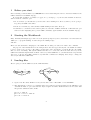
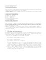
We are going to tell the CWB about the drink machines:
coffee
10p
D
10p
10p
c1
c2
Dalt
b1
10p
b2
tea
10p
coffee
tea
b3
1. Open a new file called drinks.ccs in your favourite editor. The suffix .ccs is essential.
2. The diagrams above have to be translated into the required (ccs) input syntax for the CWB. Process
declarations must be preceded with the keyword proc and since channel names can not start with
integers the definition will look like:
proc D = tenP.C1
proc C1 = tea.D + tenP.C2
proc C2 = coffee.D
2
proc
proc
proc
proc
Dalt
B1 =
B2 =
B3 =
= tenP.B1 + tenP.B3
tenP.B2
coffee.Dalt
tea.Dalt
Type this text into your file drinks.ccs and save it.
3. In the CWB window type the load command
load drinks.ccs
You should get a response like
Execution time (user,system,gc,real):(0.006,0.000,0.000,0.013)
cwb-nc>
which means that the CWB has accepted your definitions.
To see what identifiers the CWB knows about you can use the ls command.
To see the current meaning of an identifier you can use the cat command. For example executing
cat Dalt
you should get the response
===Agent===
tenP.B1 + tenP.B3
Execution time (user,system,gc,real):(0.001,0.000,0.000,0.001)
cwb-nc>
4
Checking for process equivalence
This is done with the command eq which takes different parameters, depending on what kind of equivalence
you want to consider. Here we will consider three.
Trace equivalence This is discussed in Section 3.2 of the textbook, and is sometimes called language
equivalence in the literature. The command for checking trace equivalence is eq -S trace. So, assuming
you have loaded the file drinks.ccs, type into the CWB window
eq -S trace D Dalt
After various messages it will come back with the result
TRUE
No pain involved.
Bisimulation equivalence This corresponds to what the textbook calls strong bisimulation equivalence;
see Section 3.3. The relevant command is eq -S bisim. So type
3
10p
10p
Dralt
Dr
d1
i1
reset
reset
coffee
coffee
reset
i2
d2
dead
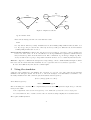
Figure 1: Explicit deadlocks
eq -S bisim D Dalt
After various messages it will come back with the result
False
Not only that it will tell you why! D satisfies the modal formula [tenP]<tenP>tt whereas Dalt does
not. If you type the processes in the other way around you will get a different reason; Dalt satisfies
<tenP>[tenP]ff whereas D does not.
Observational equivalence: This is also known as weak bisimulation equivalence, and is explained in
Section 3.4 of the textbook. It is a modification of strong bisimulation equivalence which abstracts
away as much as possible from internal actions. The command is eq -S obseq or simply eq. Try it
out if you wish. It is not going to help with D and Dalt as these do not contain any internal actions.
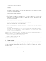
Exercise: Type into a different file descriptions corresponding to the two drink machines in Figure 1, which
have reset actions. Check that these machines are trace equivalent but not bisimulation equivalent.
2
To leave the CWB at any time use the command quit.
5
Using the simulator
Using the sim command we can simulate the execution of a process. Not quite game-arcade standard
simulation but still quite useful. Let us use it to follow the attempts of an unfortunate tea drinker to use
the faulty machine Dalt. The combined system in standard CCS is given by
(T user | T Sys)\{tenP, tea, coffee}
where Tuser is given by
def
Tuser = tenP.tea.happy.0
Here I am using the convention a for complementary actions; that is a represents output along a. Unfortunately in the CWB
• the complement of the action act is given by ’act; make sure you use the correct single quote.
• local declarations, here of tenP, tea and coffee are described using a slightly more useful notation.
The required CWB syntax is:
4
proc Tuser = ’tenP.’tea.happy.nil
set Internals = { tenP, tea, coffee}
proc TSys = (Dalt | Tuser) \ Internals
proc Dalt = tenP.B1 + tenP.B3
1. Type this syntax into your file drinks.ccs and load it once again.
2. To start the simulation execute the command sim TSys. You should get the response
TSys
1. -- t --> (B3 | ’tea.happy.nil) \ Internals
2: -- t --> (B1 | ’tea.happy.nil) \ Internals
cwb-nc-sim>
giving the two possible ways of proceeding from TSys. The CWB notation for the internal move τ is
t. Notice the special simulation prompt cwb-nc-sim. This means the CWB is in simulation mode. To
leave this mode execute quit.
3. Which track will we follow? Say the first. So execute 1. The systems responds with the next possible
moves:
(B3 | ’tea.happy.nil) \ Internals
1. -- t --> (Dalt | happy.nil) \ Internals
cwb-nc-sim>
There is only one possible way forward, again by a τ move.
4. If we follow it, by typing 1, we again get only one possible choice:
(Dalt | happy.nil) \ Internals
1. -- happy --> (Dalt | nil) \ Internals
cwb-nc-sim>
5. Trying to go further leads nowhere. Executing 1 gives
(Dalt | nil) \ Internals
The agent has no transitions
cwb-nc-sim>
We have successfully carried out the execution
τ
τ
happy
TSys −→
· −→
·−
−−→
in which the tea drinker successfully gets a cup of tea.
6. To backtrack and try other paths we can execute the command back any number of times. When we
get lost we can execute current to see the current process. For example executing back three times
and then current we should get back to:
5
TSys
1. -- t --> (B3 | ’tea.happy.nil) \ Internals
2: -- t --> (B1 | ’tea.happy.nil) \ Internals
cwb-nc-sim>
From here we can start investigating the second branch. This does not lead far. Executing 2 leads to
(B3 | ’tea.happy.nil) \ Internals
The agent has no transitions
cwb-nc-sim>
This represents a deadlocked state. The user can never get around to executing happy.
Exercise: Design a coffee-drinking process, similar to Tuser, and use the simulator to check how it fares
with the faulty Dalt.
2
Another useful command which helps in figuring out the transition system is compile. Executing
compile TSys generates the LTS and attempts to display it textually. Try it out. You will get a four
state machine. Can you understand the CWB way of describing an LTS? Draw it out on a piece of paper.
For many systems the LTS will be enormous. The command min minimises it with respect to an equivalence. The default is observational equivalence, which abstracts away from internal actions. For example
executing min TSys minTSys minimises TSys with respect to observational equivalence and assigns the resulting lts to minTSys. Try it out. Then execute compile minTSys. You should get a three state machine
which is observationally equivalent to TSys. Again draw it out on a sheet of paper.
6
More on workbench syntax
We have already seen that the input syntax for the CWB is a little different than the syntax of CCS as it
appears in the textbook, and in the literature. But it does support relabelling, as explained in the textbook,
and so does allow a modest form of parametrised definitions. For example suppose we are interested in the
system
def
T B = (Bic | Bco)\{c}
where the components are given by
def
Bic = in.c.Bic
def
Bco = c.out.Bco
Here is what the contents of an input file might look like:
*************************
* Two Buffers
**************************
proc B1 = in.’c.B1
proc B2 = c.’out.B2
*************************
* Placed together
6
****************************
proc TB = (B1 | B2) \ {c}
****************************
****************************
Here we have spelled out the definitions of the individual buffers directly as definitions B1 and B2 and then
constructed the composite system from these two components.
But we could use relabelling to emphasise that the two components share the same structure. In CWB
syntax we could write:
*******************************
****Two Buffers ***************
*** Defined by relabelling *****
proc Bgen = in.’out.Bgen
proc Bic = Bgen[c/out]
proc Bco = Bgen[c/in]
*******************************
** Placed together ***
proc TBr
= (Bic | Bco) \ {c}
*******************************
******************************
Here we have given one definition of a general buffer, and defined two instances of it, by relabelling the
actions. Note that the CWB syntax for relabelling is [acta/actb] where acta,actb are two action names;
that is complements ’act can not appear in relabellings. And of course more than one relabelling can be
made at a time, as in [a/b,c/d,e/f].
Exercise: Use the CWB to show that the two versions of a two place buffer TB and TBr are bisimilar. 2
It is a question of style as to which approach should be used in general; explicit definitions, or parametrised
definitions via relabelling.
7
Checking modal properties
The CWB also allows you to check if a process has a certain property. These properties can be written in a
large number of different logics but here we look at the simple modal logic discussed in the lectures. These
properties must be written into files whose suffix is .mu. This is essential.
1. Type into a file called drinks.mu the following list of properties:
prop cofftea1 = <tenP>(<tenP>tt /\ <tea>tt)
prop cofftea2 = [tenP](<tenP>tt)
prop cofftea3 = [tenP]([tea]ff \/ [tenP]ff)
A property definition must start with the keyword prop. Here we define three different properties,
cofftea1, cofftea2 and cofftea3. Note the ASCII syntax for the logical connectives. For example
true and false is rendered as tt and ff respectively, while the Boolean connectives are constructed
using the forward and backward clash operators / and \. Negation is rendered using the keyword not.
2. Load the file into the CWB by executing the command load drinks.mu. If it is accepted the CWB
now knows about three process properties. Again you can check what the CWB knows about by
executing ls. Do this. The list should now include
7
===Mu-Calculus and CTL Formula===
cofftea1
cofftea2
cofftea3
The definitions associated with a property name can be checked with the cat command. For example
executing cat cofftea2 will result in
===Mu-Calculus and CTL Formula===
[tenP]<tenP>tt
3. The command for checking a process with respect to a property is chk. So to see if the process D
satisfies the property cofftea1 you execute the command chk D cofftea1. The system responds,
after various messages, with
TRUE, the agent satisfies the formula.
If on the other hand chk Dalt cofftea1 is executed it responds with
FALSE, the agent does not satisfy the formula.
4. There are many languages for defining process properties. So the general form of the chk command is
chk -L lang
The default lang is mu (standing for the mu calculus) and therefore the command chk is equivalent to
chk -L mu. Some of the other languages, or features of them, will be covered in the lectures. Details
may also be found in the CWB manual.
Exercise: Find out which of the formulae cofftea2 and cofftea3 the processes D and Dalt satisfy.
2
Exercise: Referring to the reset drink machines given in Figure 1:
• Find a formula which is satisfied by D and not Dalt
• Find one satisfied by Dalt and not D.
Check your answers with the CWB.
8
2
Using scripts
When using the CWB it is often necessary to execute the same list of commands over and over again. This
occurs when you are developing a specification or perhaps investigating some implementation description.
Scripts are a convenient way of organising this activity. A list of CWB commands is placed in a file called
foo.cws and then the command es foo.cws executes all the commands in the file foo.cws. Let us go
through an example.
1. In a file called drinks.cws type in the commands
8
load drinks.ccs
load drinks.mu
eq -S trace D Dalt
eq -S bisim D Dalt
chk D cofftea1
chk Dalt cofftea1
Again the suffix .cws is essential.
2. Execute the command es drinks.cws. If the files mentioned, drinks.ccs and drinks.mu exist, that
is are in the current directory, they are loaded and the four commands are executed in turn. Try it!
3. It is often useful to keep the outcome of processing a script. This is catered for by the more general
form of the es command.
Execute the command es drinks.cws drinks.cws.output. This requests the output from running
the commands in drinks.cws to be placed in the file drinks.cws.output.
4. Now bring up the file drinks.cws.output in your favourite editor. It should contain an trace of all
the output from the CWB, while executing the commands.
When working on non-trivial examples you should always use scripts, in order to keep track of what you
are doing.
9