Download MLAB Beginner`s Guide Manual

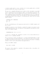
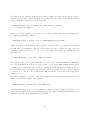
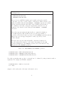
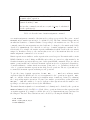
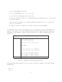
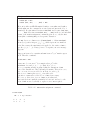
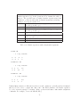
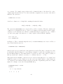
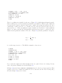
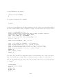
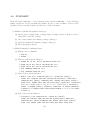
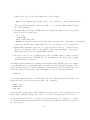
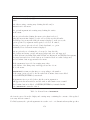
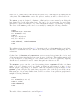
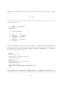
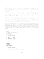
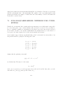
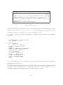
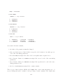
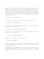
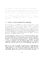
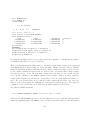
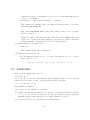
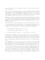
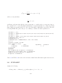
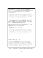
* FUNCTION LP(X,Y,Z) = (X^P+Y^P+Z^P)^(1/P)
with arguments X, Y, Z and the single parameter P. In these examples, parameters in the functional
form are represented by MLAB identifiers. When the FUNCTION command is executed, these
MLAB identifiers may be unknown or correspond to any MLAB data. However, all the parameter
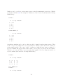
identifiers must be made into MLAB scalars before curve-fitting. For example, the commands:
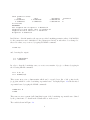
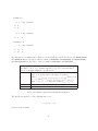
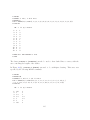
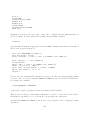
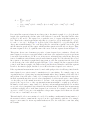
* C1 = 1; C2 = -1; A = -.07; B = -2.16
would accomplish the second step of the model setup for the functional form F above by assigning
numerical values to all the parameters of F. Similarly, P must be made an MLAB scalar before
curve-fitting the LP model above. Failure to assign numerical values to parameters in a functional
form is a common error. Some guesses must be made no matter how ill-prepared one is to do so.
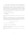
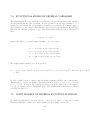
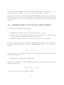
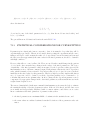
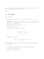
For formulating models having several functional forms to be fit simultaneously, the first step
is accomplished by transcribing each functional form into an MLAB FUNCTION command. For
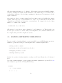
example, the model in Section 7.5 is set up as shown in the commands:
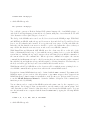
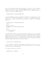
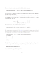
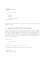
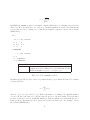
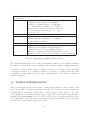
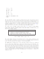
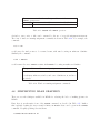
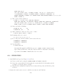
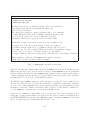
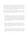
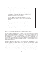
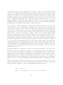
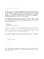
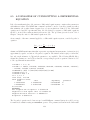
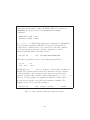
* FUNCTION X(T) = (A0*K1/(K2-K1))*(EXP(-K1*T)-EXP(-K2*T))
* FUNCTION B(T) = A0*(1.0-EXP(-K1*T)) - X(T)
with the argument symbol T, unknown parameters K1 and K2, and the fixed parameter A0. The
second step is accomplished by assigning appropriate numerical values to A0, K1, and K2. For
example:
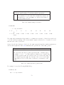
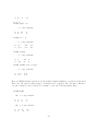
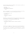
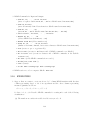
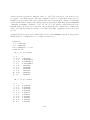
* A0 = 200; K1 = .05; K2 = .0001
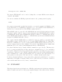
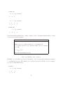
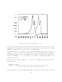
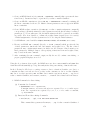
The third step is accomplished, if necessary, by creating a constraint set. For example:
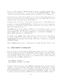
* CONSTRAINTS CS = {K1 > 0,K2 > 0}
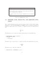
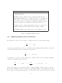
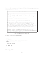
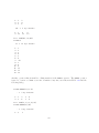
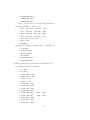
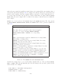
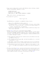
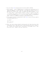
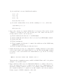
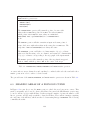
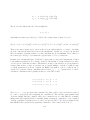
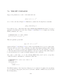
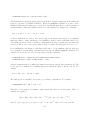
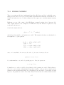
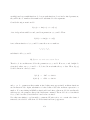
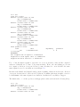
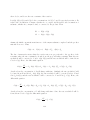
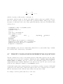
Using the correct strategy in defining complex functional forms is very important. Take, for
example, the equation:
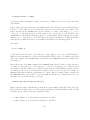
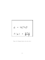
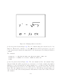
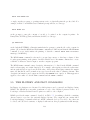
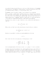
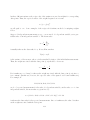
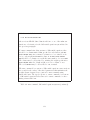
B(t) = [S(R − B0 ) − R(S − B0 ) · e−d·K1 ·t ]/[R − B0 − (S − B0 ) · e−d·K1 ·t ]
where R = (A + d)/2, S = (A − d)/2, d = (A2 − 4 · F0 · G0 )1/2 , and A = F0 + G0 + K2 /K1 .
254