Download User Manual Dracula

User Manual
Dracula
Revision : 1.6
graph masters
Bernd
Stefan
Jochen
Stefan
Matthias
Tim
Albert
Dudzik
Einhorn
Göller
Hub
Schönleber
5th December 2003
Contents
1. Getting started
7
1.1. What is Dracula? . . . . . . . . . . . . . . . . . . . . . . . . . . . . . . .
7
1.2. Starting Dracula . . . . . . . . . . . . . . . . . . . . . . . . . . . . . . . .
7
1.2.1. Command line options . . . . . . . . . . . . . . . . . . . . . . . .
8
2. Installation
9
2.1. System requirements . . . . . . . . . . . . . . . . . . . . . . . . . . . . .
9
2.2. Install from binary package . . . . . . . . . . . . . . . . . . . . . . . . .
9
2.3. Install from source code . . . . . . . . . . . . . . . . . . . . . . . . . . .
10
3. The Dracula user interface
11
3.1. The Main Console . . . . . . . . . . . . . . . . . . . . . . . . . . . . . . .
12
3.2. The Graph Box . . . . . . . . . . . . . . . . . . . . . . . . . . . . . . . . .
12
3.3. The Analyzer . . . . . . . . . . . . . . . . . . . . . . . . . . . . . . . . .
12
3.4. The Graph Windows . . . . . . . . . . . . . . . . . . . . . . . . . . . . .
13
4. Working with projects
15
4.1. Creating a new project . . . . . . . . . . . . . . . . . . . . . . . . . . . .
15
4.2. Loading a project . . . . . . . . . . . . . . . . . . . . . . . . . . . . . . .
15
4.3. Saving a project . . . . . . . . . . . . . . . . . . . . . . . . . . . . . . . .
16
5. Working with graphs
17
5.1. The Default Graph . . . . . . . . . . . . . . . . . . . . . . . . . . . . . .
17
5.2. Creating new graphs . . . . . . . . . . . . . . . . . . . . . . . . . . . . .
17
5.3. Renaming and deleting graphs . . . . . . . . . . . . . . . . . . . . . . .
18
5.4. Exploring graphs . . . . . . . . . . . . . . . . . . . . . . . . . . . . . . .
18
5.4.1. Scrolling . . . . . . . . . . . . . . . . . . . . . . . . . . . . . . . .
19
5.4.2. Zooming . . . . . . . . . . . . . . . . . . . . . . . . . . . . . . . .
19
5.4.3. The Minimap . . . . . . . . . . . . . . . . . . . . . . . . . . . . .
19
5th December 2003: 8:48
3
5.5. Changing graph layout . . . . . . . . . . . . . . . . . . . . . . . . . . . .
20
5.5.1. Manual layout . . . . . . . . . . . . . . . . . . . . . . . . . . . . .
20
5.5.2. Builtin layouts . . . . . . . . . . . . . . . . . . . . . . . . . . . . .
20
5.5.3. Custom layouts . . . . . . . . . . . . . . . . . . . . . . . . . . . .
21
5.6. Getting information about nodes . . . . . . . . . . . . . . . . . . . . . .
21
5.6.1. Showing attributes . . . . . . . . . . . . . . . . . . . . . . . . . .
21
5.6.2. The Info cursor . . . . . . . . . . . . . . . . . . . . . . . . . . . .
22
5.6.3. Showing the sourcecode . . . . . . . . . . . . . . . . . . . . . . .
22
5.7. Selections . . . . . . . . . . . . . . . . . . . . . . . . . . . . . . . . . . . .
22
5.7.1. The Working Selection . . . . . . . . . . . . . . . . . . . . . . . .
22
5.7.2. Selecting and deselecting nodes . . . . . . . . . . . . . . . . . .
22
5.7.3. Stored Selections . . . . . . . . . . . . . . . . . . . . . . . . . . .
23
5.7.4. Creating new Stored Selections . . . . . . . . . . . . . . . . . . .
23
5.7.5. Editing and deleting Stored Selections . . . . . . . . . . . . . . .
23
5.7.6. Transforming Stored Selections . . . . . . . . . . . . . . . . . . .
24
5.8. Markings . . . . . . . . . . . . . . . . . . . . . . . . . . . . . . . . . . . .
24
5.8.1. Marking and unmarking nodes . . . . . . . . . . . . . . . . . . .
24
5.9. Modifying a graph . . . . . . . . . . . . . . . . . . . . . . . . . . . . . .
24
5.9.1. Showing & hiding nodes . . . . . . . . . . . . . . . . . . . . . . .
25
5.9.2. Deleting nodes . . . . . . . . . . . . . . . . . . . . . . . . . . . .
25
5.9.3. Predecessors & successors . . . . . . . . . . . . . . . . . . . . . .
25
6. Advanced graph operations
6.1. Building new graphs from existing ones . . . . . . . . . . . . . . . . . .
27
6.1.1. Merging graphs – union, intersection, difference . . . . . . . . .
27
6.1.2. Cloning Working Selections . . . . . . . . . . . . . . . . . . . . .
28
6.2. Controlling edge visibility . . . . . . . . . . . . . . . . . . . . . . . . . .
28
6.3. Using filters . . . . . . . . . . . . . . . . . . . . . . . . . . . . . . . . . .
29
6.3.1. Simple Filters . . . . . . . . . . . . . . . . . . . . . . . . . . . . .
29
6.3.2. Predefined Filters . . . . . . . . . . . . . . . . . . . . . . . . . . .
30
6.4. Annotations . . . . . . . . . . . . . . . . . . . . . . . . . . . . . . . . . .
30
6.5. Exporting graphs . . . . . . . . . . . . . . . . . . . . . . . . . . . . . . .
31
7. Usage of the Dracula Scripting Language (DSL)
4
27
33
7.1. Loading a scripting file and how it is parsed . . . . . . . . . . . . . . .
33
7.2. Composition and syntax of DSL . . . . . . . . . . . . . . . . . . . . . . .
33
5th December 2003: 8:48
7.2.1. Key Words . . . . . . . . . . . . . . . . . . . . . . . . . . . . . . .
33
7.3. The commands and examples for them . . . . . . . . . . . . . . . . . .
34
7.4. The node sets . . . . . . . . . . . . . . . . . . . . . . . . . . . . . . . . .
37
7.4.1. Constraints for node sets
. . . . . . . . . . . . . . . . . . . . . .
8. Customizing Dracula
38
39
8.1. Program Configuration . . . . . . . . . . . . . . . . . . . . . . . . . . . .
39
8.1.1. Structure of the Program Configuration file . . . . . . . . . . . .
39
8.2. Node Type Configuration . . . . . . . . . . . . . . . . . . . . . . . . . .
43
8.2.1. Structure of the Node Type Configuration file . . . . . . . . . .
43
8.3. Edge Group Configuration . . . . . . . . . . . . . . . . . . . . . . . . . .
44
8.3.1. Structure of the Edge Group Configuration file . . . . . . . . . .
45
A. Custom layouts Howto
47
A.1. How the mechanism works . . . . . . . . . . . . . . . . . . . . . . . . .
47
A.2. Design guidelines for layouters . . . . . . . . . . . . . . . . . . . . . . .
47
A.3. Notes on the structure of the input and output files . . . . . . . . . . .
48
A.4. Example . . . . . . . . . . . . . . . . . . . . . . . . . . . . . . . . . . . .
48
5th December 2003: 8:48
5
6
5th December 2003: 8:48
1. Getting started
In this chapter you will learn what Dracula is and what it is used for and how you
begin working with it. First we will discuss what Dracula allows you to do. Then we
show you how Dracula is started and which options you have when starting it.
1.1. What is Dracula?
As of the name “Dracula” you may expect that this program must have something to
do with vampires. It does not. Maybe it would sometimes be a horror to work with
it, but hopefully not. So what is Dracula then?
Dracula is a system to visualize an IML-graph which was created using the tools from
the Bauhaus Project developed at the University of Stuttgart. Such an IML-graph is
an intermediate representation of the sourcecode of a certain software system. Here
is a short overview of the functions Dracula provides:
• creating subgraphs (called “graphs”) of an IML-graph which can be viewed on
screen
• many tools to explore those graphs (like scrolling, zooming etc.) and manipulating them (e.g. hiding or adding certain nodes etc.)
• full control over the layout and the appearance of nodes and edges in the graphs
• a powerful scripting language (the DSL) for executing all functions of the system by script commands
• and much more. . .
You may ask how the hell did they come to this strange name “Dracula”? Ok, let us
try to explain it. The word “graph” which Dracula is all about as you know already
sounds very similar to the german word “Graf”. And “Graf” is the german word for
“count”. Now, one of the most famous counts is of course count “Dracula”, so this
name was chosen for the system.
1.2. Starting Dracula
You may think that starting Dracula should be a simple task and indeed it is. Just
change into the directory where Dracula was installed to and type
5th December 2003: 8:48
7
./dracula
into your console and you should see some windows appearing on the screen (provided that Dracula was correctly installed and your system meets the minimum requirements). Besides simply starting Dracula this way, you may also provide some
command line options which will be described in the following section.
1.2.1. Command line options
There are four optional command line parameters you may specify when starting
Dracula:
./dracula [config-file] [project-file] [scripting-file] [-v(0-4)]
• Paramter “config-file”
If you do not want the default Program Configuration to be used, you may
provide the path and filename to another one here (Important note: the suffix
of the configuration file must be “.dcf” or it will not be correctly recognized as
a Program Configuration file by Dracula). More about configuration files and
customization of Dracula can be found in chapter 8.
• Parameter “project-file” You can directly load a previously saved project when
starting dracula by specifying the path and filename of the project file on the
command line. (Important note: the suffix of the configuration file must be
“.dpf” or it will not be correctly recognized as a project file by Dracula). You
will learn more about projects in chapter 4.
• Parameter “scripting-file” Most of the functionality of Dracula can be invoked
by script commands denoted in the Dracula Scripting Language (DSL). When
starting Dracula you can specify the path and name of a file containing one or
more of these scripting commands. All the commands in the file are then executed directly after Dracula has been started. More information about scripting,
scripting files and the DSL can be found in chapter 7.
• Parameter “-v” This parameter defines the level of verbosity (or debug level)
for debug messages written to the console. “-v0” for example means that there
should be no messages at all. “-v1” only shows critical messages. “-v2” shows
critical and warning messages. “-v3” and “-v4” give even more messages. As
you can see a higher debug level includes all messages that are written at lower
levels, too.
8
5th December 2003: 8:48
2. Installation
This chapter describes how to install Dracula on your system. First we will give some
hints about the system requirements Dracula needs to work. Then you will learn how
to install Dracula from a binary package. The last section is about compiling and
installing Dracula dircectly from source code.
2.1. System requirements
Dracula is written in Ada 95 and uses the Gimp Toolkit (GTK) for its graphical user
interface. So it is able to run on a variety of platforms from which actually Linux and
Sun Solaris systems are supported (other platforms will maybe need some changes
to the source code).
Recommended system:
• CPU: fast processor (1GHz or more)
• RAM: 512Mb or more (the bigger the graphs are you want to work with, the
more RAM you should have, because swapping is soooo sloooow)
• HDD: around 15Mb (for Dracula only)
• GTK+ 2.2.0 (or higher) libraries installed
2.2. Install from binary package
Installing Dracula from a binary package is a simple task. First check that you have
got the right package for your platform and that your platform meets the requirements. Move the file “dracula-<platform>.tar.gz” into the directory you want Dracula install to. Change to this directory and type
tar xzvf dracula-<platform>.tar.gz
to unpack it. This will create a subdirectory “dracula” in the current directory, including all the needed files. All you have to do then is starting Dracula like described
in chapter 1. Maybe you should also change the configuration files to your needs (see
chapter 8 for details).
5th December 2003: 8:48
9
2.3. Install from source code
To compile the source code you need the following tools:
• Gnat 3.15
• Aflex & Ayacc
• GtkAda 2.2.0
Note that these tools should be found in path. The sourcecode is deployed in a .tar.gzfile. First unpack it with
tar xzvf dracula-src.tar.gz
Then change into the newly created “dracula-src” directory and type
make
This will compile the source code. If done, type
make install
which will create a new directory called “dracula” inside the current directory, which
contains all necessary files and directory structure for Dracula.
10
5th December 2003: 8:48
3. The Dracula user interface
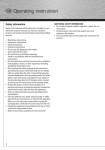
Dracula provides a graphical user interface consisting of multiple windows. After
starting Dracula at least three windows appear on the screen like shown in figure
3.1. These are the “Main Console”, the “Graph Box” and the “Analyzer”, which will
be briefly discussed in the following sections. The “Graph Window” which finally
displays a graph on screen is also explained. What we leave out here are various
dialog windows. These will be described later in conjunction with the operations
they are used for. It is assumed here that you (the reader) have basic knowledge about
computers and know how to work with graphical window-based user interfaces. So
we will not discuss here how to turn on your computer or what a mouse is.
Figure 3.1.: After Dracula has been started
5th December 2003: 8:48
11
3.1. The Main Console
The Main Console is one of the most important windows in Dracula. It is used to
create new projects, save them or load previously saved ones. More about projects
can be found in the next chapter. The window contains a main menu where various
actions can be triggered and a toolbar below it which provides buttons to serve as
shortcuts to the most important functions. Below the toolbar you will find a scrollable
list where all actions you have done so far are logged. In the titlebar of the Main
Console the filename of the current project is shown.
To exit Dracula click on the menu “Project” and choose the item “Exit”. If you want
to show the online help click on “Help|Manual...”. This will open the web browser
defined in the Program Config (see chapter 8 for details) showing this manual. The
other menu-items and the functions of the other buttons will be explained later.
Figure 3.2.: The Main Console
3.2. The Graph Box
The Graph Box gives an overview of all the graphs that are part of the current project
and allows executing differen operations on them. The listbox in the the Graph Box
contains these graphs (or better: their names) as items. The eye symbol before a
graph name indicates whether the graph is currently displayed on screen in a Graph
Window. If it is crossed then the graph is currently not shown. A click with the left
mouse button on the eye symbol switches between the two states. If there are Stored
Selections defined for a graph their names and colors will be displayed in the listbox
too. They are shown as second level items below the items that represent the graphs.
To hide them in the listbox click on the “-”-sign before the graph name or on the “+”sign to show them if they are currently hidden.
Below the listbox is a toolbar containing some buttons to execute various operations
on graphs or selections. Their functions will be described later.
3.3. The Analyzer
The Analyzer is used to display the attributes of a certain node in conjunction with
their values, when using the Info Cursor. It contains a scrollable listbox with two
columns. In the first column the name of the attributes is displayed, while the second
one includes the value of the corresponing attribute in the first column. More on the
Analyzer and the Info Cursor can be found in chapter 5.
12
5th December 2003: 8:48
Figure 3.3.: The Graph Box
Figure 3.4.: The Analyzer
3.4.
The Graph Windows
The Graph Windows display the graphs on screen and therefore will be the windows
you work with most of the time. Each Graph window displays exactly one graph. The
name of the graph is displayed in the titlebar of the Graph Window. A Graph Window
contains a toolbar on the left side of the window and a statusbar on the bottom. The
rest of the window is used by a drawing area where the graph is visualized. Left and
below this area are two scrollbars that allow to scroll the contents of the drawing area
(since the whole graph may be greater than what fits into the visible area).
A click with the right mouse-button into the drawing area will display a popup-menu
which allows you to perform different actions on the graph. If the mouse cursor is
above a node another popup-menu will be displayed with items that perform actions
on this node only.
The button “Show/Hide Toolbar” allows you to hide the toolbar to leave more space
for the drawing area which will be automatically resized. If the toolbar is hidden a
click on this button will show it again.
The statusbar at the bottom of the window shows you some important information
like how many nodes there are in the graph, how many of them are currently visible,
how many nodes are in the Working Selection and how many are currently marked.
Details about the functions of the toolbuttons and menu-items and the possibilities
5th December 2003: 8:48
13
the drawing area provides are explained in later chapters.
Figure 3.5.: A Graph Window
Figure 3.6.: The toolbar of a Graph Window
14
5th December 2003: 8:48
4. Working with projects
In this chapter you will learn more about projects and graphs. A project in Dracula
includes a certain IML-graph together with one or more subgraphs of this IML-graph.
These subgraphs are simply called “graphs” in Dracula and they are the objects you
work with most of the time in Dracula. More on graphs you will find in chapter 5.
But before you can start working with graphs you will first have to create or load a
project.
4.1. Creating a new project
To create a new project (i.e. load a new IML-graph) you can either click on the item
“Project” of the main menu in the Main Console and choose the item “New...” or
you can use the toolbutton “New Project” instead. Afterwards a file-chooser dialog is
displayed where you can choose the IML-file, where the IML-graph is contained in.
A click on the button “Ok” will then load the IML-graph. While loading a window
is displayed which shows you the progress (i.e. how many nodes have been read so
far). Depending on the graph’s size this may take a while, so be patient. After the
IML-graph was successfully loaded a Graph Window is opened showing the Default
Graph. If something goes wrong while loading the IML-graph (e.g. the file you have
chosen is not a valid IML-File), Dracula while give you an error message telling you
what the problem is. Please note also that there can only be one project openend at
any time in Dracula. So if you create a new one without saving an already existing
one you will loose all changes made so far in the existing project.
4.2. Loading a project
If you want to load a previously saved project either choose the menu-item “Project|Open...”
of the main menu in the Main Console or click the button “Open Project” in the toolbar instead. Then a file-chooser dialog is displayed where you may specify the filename of the project file. A click on the button “Ok” will then load the project. Note
that the corresponding IML-file must also be reloaded. Dracula searches for the IMLfile on the same position, where it was as the project was created. If Dracula cannot
find the IML-file or the project file was not a valid Dracula Project file, you will get an
error message. Another important fact is, that Dracula Project files always must have
the suffix “.dpf” or they will not be recognized as a project file.
5th December 2003: 8:48
15
4.3. Saving a project
After hours of hard work hand-tuning your graph’s layout you may want to save all
your work done so far and get some sleep. Of course Dracula allows you to do this.
To save a project (including all graphs, selections etc.) choose the item “Save” under
the menu “Project” in the Main Console or use the toolbutton “Save Project” instead.
If the project was previously saved or opened, then the project will be saved under
the same filename. Otherwise if you created a new project, Dracula will ask you for
a filename by opening a file-chooser dialog, where you can enter the filename. If you
want to save a project under another name than the current one you have to choose
the item “Project|Save As...”. Dracula will then display a file-chooser dialog where
you can specify the name and place of the new file and after clicking the button “Ok”
the project will be saved under the given filename. Note: since Dracula is software
and software is never entirely bug-free you should keep to the simple rule “Save
often, save much.” to minimize the risk of loosing all your work done so far.
16
5th December 2003: 8:48
5. Working with graphs
As you may already know, graphs are possibly the most important objects in Dracula.
A graph is simply a user-defined subset of all the nodes and edges of the IML-graph
in the current project. You can define as many different graphs as you wish (you are
only limited by your system’s memory). Each graph has its own unique name and
is displayed in its own Graph Window where you can explore or manipulate it in
many ways. In this chapter you will learn the basic operations on graphs, you will
need most of the time when working with Dracula. More advanced (which does not
necessarily mean more complex) operations that you may not need in your all-day
work are described in the next chapter.
5.1. The Default Graph
After creating a new project Dracula automatically creates a graph called the “Default
Graph”. The Default Graph contains exactly one node of type “System”. You can
immediately start work with this basic graph.
5.2. Creating new graphs
Maybe you do not want to work with the Default Graph Dracula automatically creates for you, but instead you want to create your own graphs (possibly with other
nodes). There are different ways in Dracula to do this. Some of them work on the basis of existing graphs, like creating differences, unions or intersections of two graphs
or creating a new graph out of a selection of nodes of another graph. These possibilities will be discussed later. Here we will focus on creating graphs from scratch.
This is a bit more complex task since it involves writing script commands in the Dracula Scripting Language (which is described in more detail in chapter 7). First, open
the Graph Box and click on the button “New Graph”. A dialog is shown with a
textfield, where you can type in the script command needed to create the graph you
want. If you wish to create a graph that contains all nodes of the current IML-graph
then type the following command into the textfield:
create graph “MyGraph” with imlnodes;
After a click on the button “Ok” and some seconds or hours later (depending on the
size of the IML-graph) a new Graph Window is shown containing the newly created
graph. There will also be a new item “MyGraph” in the listbox of the Graph Box. It
5th December 2003: 8:48
17
is important that each graph has its own unique name, so when you try to create a
graph with a name that already exists you will get an error message. Also, be careful
not to use the command as shown above together with big IML-graphs or you will
have to wait a very long time before the graph is finally displayed. Dracula is not
intended to work this way and of course you will be completly lost in a graph with
millions of nodes and even more edges. So always try to restrict the “create graph”
command to a small subset of the nodes of the original IML-graph. Chapter 7 describes how you can do this.
When creating a graph this way you also have the option to choose a Node Configuration to be used with the new graph. If you do not explicitly specify a Node
Configuration for the graph, Dracula uses a default one. The Node Configuration
tells Dracula how to draw the nodes of that graph in the Graph Window. To be more
specific it sets the colors of the nodes, their icons and the attributes to be displayed
inside the nodes. For more details about the Node Configuration refer to chapter 8.
To create a graph with your own Node Configuration you have to tell Dracula which
Node Configuration file it should use, like in the following command:
create graph “MyGraph” with imlnodes using “mynodeconfig.ncf”;
This command would create a graph named “MyGraph” which contains all nodes
of the current IML-graph. Moreover it would use the Node Configuration stored in
the file “mynodeconfig.ncf” in the current path, instead the default Node Configuration as in the example above. Please notify, that once you have created a graph you
cannot change its Node Configuration afterwards.
5.3. Renaming and deleting graphs
After a graph has been created you can change its name in the following way: select
the graph to rename in the listbox of the Graph Box and then click the button “Rename
Graph”. A dialog with an edit-field appears where you can type in the new name.
After you press the “Ok” button the graph will be renamed to the name you specified,
except when there is already another graph with the same name in which case you
get an error message.
When the time comes that you no longer need a particular graph you may delete it.
To do that, select the graph in the listbox of the Graph Box and click on the button
“Delete Graph/Selection”. Be careful, because Dracula will not ask you to confirm,
but delete the selected graph immediately.
5.4. Exploring graphs
Graphs could get very big, although you should limit their size as discussed before.
This means that a graph normally cannot be displayed completely in the drawing
area of its Graph Window. Most of the graph will lie outside of the visible area. To
see the other parts of the graph you may scroll the drawing area. Or you may zoom
into or out of the graph too see more details or to get a better overview of it.
18
5th December 2003: 8:48
5.4.1.
Scrolling
Scrolling can be done in three different ways. The first one is by using the scrollbars
next to and below the drawing area in the graph window. The vertical bar will scroll
the drawing area vertically while the horizontal bar will scroll it horizontally (as you
may have already guessed). The indicators in the bars show you how much of the
graph is currently displayed in the drawing area and which position you currently
look at. To scroll you can either drag&drop the indicators to a new position or click
on the arrows in the scrollbars to move a step into the desired direction.
Another way to scroll the graph is the Hand Cursor. To activate it either use the
button “Hand Cursor” in the toolbar of the Graph Window or press the key “h”.
Then move the mouse cursor above the drawing area (you will notice that it changes
to a little hand) and press the left mouse button and hold it. Now when you drag
the mouse around the drawing area will be scrolled into the direction you move the
mouse to. To leave the Hand Cursor mode press the “Standard Cursor” button or
press the key “d”.
The third possibility to scroll is the Minimap which will be explained below.
5.4.2.
Zooming
Sometimes you want to get a better overview of the graph, or you want to see more
details. This can be achieved by zooming out of or into the graph. To zoom into it
click the button “Zoom in” in the toolbar of the Graph Window or right-click into
the drawing area (be sure that the mouse cursor is not above a node) and choose the
menu-item “Zoom|Zoom In” in the popup-menu.
To zoom out of the graph instead click the button “Zoom out” in the toolbar or rightclick into the drawing area (again the mouse cursor must not be above a node) and
choose the menu-item “Zoom|Zoom out” in the popup-menu.
If you have zoomed to much into or out of the graph and now you want to get back
to the normal zoom level you can click either on the button “Zoom 1:1” in the toolbar
or choose the popup menu-item “Zoom|Zoom 1:1”.
5.4.3.
The Minimap
The Minimap on the left side of the Graph Window (right above the “Zoom” buttons)
gives you an overview of the size of the current graph. The white area symbolizes the
total area the graph takes up. The black rectangle inside the minimap symbolizes
which part of the graph is currently visible in the drawing area and how big it is in
relation to the whole graph. Please note, that this rectangle may look distorted, e.g.
like a line or simply a point, if the graph is distorted in some way (e.g. a hundred
times as long as high) or if it is very big in size.
Besides showing an overview of the graph, the Minimap can also be used to scroll
the drawing area. Just click into the Minimap with the left mouse button and hold it.
Then move the mouse, and you will see the rectangle in the Minimap following your
moves. At the same time the contents of the drawing area (i.e. the graph) are scrolled
to the new position, that is symbolized by the rectangle in the Minimap.
5th December 2003: 8:48
19
5.5. Changing graph layout
After a new graph is created it is displayed inside the Graph Window in a grid-like
manner (i.e. the nodes are ordered in columns and lines). Most often this standard
layout is not a good one, because important edges lie beneath nodes and it is not easy
to find structures in the graph. So you want to change the positions of the nodes to
better reflect these structures. Dracula gives you three different options to do this,
which will be described here. Note that only the positions of nodes can be changed,
the edges on the other hand will alway go straight from one node to another.
5.5.1. Manual layout
The most flexible way to change the layout of a graph is – of course – the manual
way. This means, that you change the positions of the nodes by hand. To do that, first
check that you currently use the Standard Cursor (if not press the key “d” or click on
the button “Standard Cursor” in the toolbox of the Graph Window). Then left-click
on the node in the drawing area and move the mouse while holding the left mouse
button down. The node will follow your movements. As soon as the node is in the
desired position release the mouse button and the node will be placed there.
If you want to change the position of a group of nodes, instead of moving each single
node seperately you will first have to create a Working Selection including these desired nodes. Then, if you move one of the nodes like described above, all the nodes
in the selection will be moved together while retaining their relative positions to each
other. Informations about selections and creating a Working Selection can be found
later in this chapter.
5.5.2. Builtin layouts
Creating a manual layout by moving single nodes is a time-consuming task, especially with greater graphs. Therefore Dracula provides a way to automatically position all the nodes in a graph at once. Three such layouts (called “builtin layouts”) are
integrated in Dracula: the Grid Layout, the Circle Layout and the Tree Layout.
The Grid Layout is the standard layout a graph has after it is created. The nodes are
aligned in columns and edges. To apply the Grid Layout to a graph simply click on
the button “Grid Layout” in the toolbox of the Graph Window or right-click (the cursor must not be above a node) into the drawing area and select “Layout|Grid” from
the popup-menu.
The Circle Layout positions all nodes on a circular path. The size of the circle depends
on the amount of nodes and their size. So it is only useful for smaller graphs. To apply the Circle Layout click on the button “Circle Layout” in the toolbox of the Graph
Window or click with the right mouse button into the drawing area and choose the
menu-item “Layout|Circle” from the popup-menu.
The third builtin layout is the Tree Layout. It positions the nodes of the graph in a
tree-like manner. Normally this layout would work best with graphs that are in fact
trees. But it will work also with other graphs, that contain circles for example. To
apply the Tree Layout just click the button “Tree Layout” in the toolbox of the Graph
Window or instead right-click the drawing area (while not above a node) and choose
20
5th December 2003: 8:48
the item “Layout|Tree” from the popup-menu that appears.
Always be careful when applying a builtin layout because the original layout will be
destroyed and Dracula will not ask you to confirm your choice. And unfortunately
there is no undo-function in Dracula. . .
5.5.3.
Custom layouts
Although the builtin layouts are powerful ones, they may not be exactly what you
want. In this case Dracula provides you another option: you can write your own layout algorithms (we call them “custom layouts”) and use them as a plugin in Dracula.
Basically these algorithms are provided in the form of external executable programs
which are able to interface with Dracula. When applying a custom layout Dracula
sends information about which nodes and edges exist to the external program. Then
the external program calculates the new node positions and returns them back to
Dracula. Finally Dracula layouts the graph according to this information. How exactly this mechanism works and to which conventions the external program has to
comply to is described in appendix A.
Now, to apply a custom layout to a graph either click on the button “Custom Layout” in the toolbox of the Graph Window or choose the item “Layout|Custom” in
the popup-menu, which appears when clicking with the right mouse button in the
drawing area. Then a dialog is shown, which allows you to choose one of the available custom layouts (which custom layouts exist is defined in the Program Config see chapter ?? for details). Choose the desired layout by selecting it in the combobox
of the dialog and click on the button “Ok”. After a short while the graph is updated
to the new layout. Otherwise, if something goes wrong you will get an error message.
5.6.
Getting information about nodes
As you may already know, the nodes in Dracula are not just simply nodes but represent some part of the sourcecode of a particular software system. Each node normally
has attributes attached to it, which provide some additional information (besides the
type of the node). Some of these attributes may be displayed right inside the node’s
body in the Graph Window. Dracula provides some facilities to view the attributes of
a node all at once and to show the sourcecode corresponding to a node.
5.6.1.
Showing attributes
To show the attributes of a certain node in a separate window right-click on the node
and choose the item “Attributes...” from the popup-menu. A new window similar
to the Analyzer will appear, which shows you all attributes of the node and their
values. Note that this window will stay on screen until you click the “x” button in the
window’s titlebar. This allows you to easily compare the attributes of different nodes.
5th December 2003: 8:48
21
5.6.2. The Info cursor
Another way to get the attributes of nodes is the Info Cursor which works a bit different than the former method. To use it click the button “Info Cursor” in the toolbar
of the Graph Window or press the key “i”. When you move the mouse above the
drawing area you will notice the mouse cursor changing to some king of question
mark. If you left-click on a node with the Info Cursor the attributes of that node are
displayed in the Analyzer and stay there until you click on another node. To leave
the Info Cursor mode again click the button “Standard Cursor” or press the key “d”.
5.6.3. Showing the sourcecode
You are also able to view the sourcecode corresponding to a particular node, provided that the node has a corresponding line in the sourcecode (i.e. it is not artificial)
and the sourcecode can be located. Since the filename of the sourcecode file is got
from an attribute “Filename” of a node, the sourcecode must be in the same place as
it was when the IML-graph was created. To show the sourcecode of a node right-click
on it and choose the item “Show sourcecode...” from the popup-menu. If the above
preconditions are met then an editor (which one, is controlled by the Program Config - see chapter 8) is started showing the exact position in the sourcecode file that
corresponds to the node.
5.7. Selections
Selections allow you to define groups of nodes, either to execute some special function on all nodes of the group (like moving all together as shown earlier in this chapter) or just to indicate that they belong together. Dracula distinguishes between two
types of selections - the Working Selection and the Stored Selections. Selections are
defined graph-wide, which means that different graphs have different independent
selections.
5.7.1. The Working Selection
In each graph exists at most one so-called Working Selection. A node that belongs to
the Working Selection is highlighted with a red border around it. There are also some
functions in Dracula which operate exclusively on the Working Selection.
5.7.2. Selecting and deselecting nodes
To define the Working Selection and to add or remove nodes from it, you may use
the Select Cursor. To get it click on the button “Select Cursor” in the toolbar of the
Graph Window or press the key “s” instead. If you left-click on a node with the
Select Cursor enabled the node will be added to the Working Selection. If it already
belongs to the Working Selection it will be excluded from it. Another possibility is
selecting nodes by drawing up a rectangle with the Select Cursor. Just left-click on the
22
5th December 2003: 8:48
space between the nodes and hold the mouse button. Then move the mouse to draw
up the rectangle. When you release the mouse button all nodes that are completely
contained in the rectangle are added to the Working Selection.
A fast way to select or deselect all nodes of a graph at once is right-clicking in the
drawing area (not on a node) and choosing the menu-items “Select all” or “Deselect
all” from the popup-menu.
5.7.3.
Stored Selections
Stored Selections are different from the Working Selection in that there can be more
than one Stored Selection per graph and you normally do not operate on them directly. Think of them as a kind of saved Working Selection, because you can create
a Stored Selection out of the Working Selection. Then you may modify the Working
Selection and if you want to get the original Working Selection back you may transform the Stored Selection back to the Working Selection. Since you can assign each
Stored Selection its own color and name it is a great tool for building groups of nodes
to show that they belong together. If a node belongs to a Stored Selection it gets highlighted with a border around it in the color defined for the selection. Of course a node
can belong to as many Stored Selections as you wish. Which Stored Selections there
are defined in a graph can be seen in the listbox of the Graph Box, where the Stored
Selections are displayed with their name and color as subitems beneath the graphs.
5.7.4.
Creating new Stored Selections
To create a Stored Selection you need a Working Selection first, because the Stored
Selection is formed out of the Working Selection. Click on the button “New Selection”
in the toolbar of the Graph Window or right-click in the drawing area and choose the
menu-item “New Selection...” from the popup-menu to open the “Specify Selection”
dialog. In this dialog enter the name of the new selection into the textfield and choose
the desired color for the selection in the color-chooser. Be sure to use a name different
from the names of the other Stored Selections of the same graph, or you will get an
error message. When you have finished click on the button “Ok” to create the new
Stored Selection.
5.7.5.
Editing and deleting Stored Selections
If you want to change the name and/or color of a Stored Selection select the desired
Stored Selection in the listbox of the Graph Box and click the button “Edit Selection”.
The “Specify Selection” dialog appears with the current values for name and color of
the selection. Change it as you wish and click the button “Ok” to apply your changes
to the Stored Selection.
A Stored Selection that is not used any more can be deleted by selecting it in the
Graph Box and clicking on the button “Delete Graph/Selection”. This will delete the
selection immediately, so be careful.
5th December 2003: 8:48
23
5.7.6. Transforming Stored Selections
You can transform a Stored Selection into the Working Selection which means that
the Working Selection includes all the nodes of the Stored Selection and only them
afterwards. This works as follows: choose the appropriate Stored Selection in the
Graph Box and click the button “Transform Selection”. The transformation will not
destroy the Stored Selection.
5.8. Markings
Markings are another way to group and highlight nodes. What distinguishes them
from selections is, that there are no operations that work specifically on them but
more important that they are defined project-wide instead of graph-wide. That means
that if a node is marked in one graph, the same node is automatically marked in all
other graphs of the project too. So we can say that there is always at most one marking
in a project. Marked nodes are decorated by a little green flag above the upper right
corner.
5.8.1. Marking and unmarking nodes
Marking or unmarking nodes is normally done with the Mark Cursor. To use it click
the button “Mark Cursor” in the toolbox of the Graph Window or press the key “m”
instead. A left-click on a node will then add it to the marking or remove it, if it is
already marked. You can also draw up a rectangle to add more than one node at
once to the marking. Just press the left mouse button when the cursor is over the
space between the nodes and hold it. Then move the mouse to draw up the rectangle
around the nodes you wish to mark. As soon as you release the mouse button all
nodes that lie completely inside the rectangle will be added to the marking.
To mark or unmark all nodes at once right-click into the drawing area and choose the
item “Mark all” or “Unmark all” from the popup-menu.
5.9. Modifying a graph
Until now we did only change the graphical representation of the graph, but we never
changed the graph’s contents itself after it was created. Which facilities Dracula provides to change the contents of the graph are discussed here. In general you are able
to hide or show certain nodes in the graph or to add or delete nodes. Note that this
distinguishment is more a formal one. Whether you just hide a node or delete it will
have the same visual effects: in both cases the node will not be displayed in the Graph
Window any more. The usage of filters to show and hide nodes is explained in the
next chapter.
24
5th December 2003: 8:48
5.9.1.
Showing & hiding nodes
To hide a node click on it with the right mouse button. In the popup-menu appearing
choose the item “Hide Node”, to make the node and all edges attached to it invisible.
Remember, that a hidden node still belongs to the graph, you just can not see it. This
can be realized easily when applying one of the builtin layouts for example. You will
notice that you get “holes” in these layouts where the hidden nodes would normally
been placed.
To make all hidden nodes visible again right-click into the drawing area of the Graph
Window and select the item “Show All” from the popup-menu.
5.9.2.
Deleting nodes
Instead of just hiding a node it can also be completely removed from the graph. This
can be achieved by right-clicking on the node and choosing the menu-item “Delete
Node” from the popup-menu.
It is also possible to remove all the nodes in the current Working Selection at once,
by either right-clicking in the drawing area of the Graph Window and choosing the
item “Delete Selected Nodes” in the popup-menu or by clicking the button “Delete
Selected Nodes” in the toolbar.
Deleted nodes cannot be reintroduced into the graph by the “Show All” operation
explained before.
5.9.3.
Predecessors & successors
Dracula allows you to show or hide all predecessors or successors of a node at once.
Click on the node with the right mouse button and choose the item “Predecessors /
Successors” from the popup-menu that appears. This will open the “Predecessors /
Successors” dialog. There you first have to specify how many edges to follow to get
the predecessors or successors. Enter the desired number into the textfield “Layer”.
Now you choose the operation you want to carry out. When you want to show predecessors click the button “Show Predecessor”, else if you want to hide predecessors
click the button “Hide Predecessor”. The same works for successors by clicking on
the button “Show successor” or “Hide successor” buttons. Two important remarks:
first, if the successors or predecessors to be shown are not already part of the graph,
they will first be added to it. But if they are hidden again, they will not be removed
automatically. Second, the node which you clicked on will never be hidden by these
operations, even if there is a cycle in the graph which leads back to the node (i.e. the
node is its own predecessor and successor at the same time).
5th December 2003: 8:48
25
26
5th December 2003: 8:48
6. Advanced graph operations
In this chapter we will discuss some other operations that can be carried out on
graphs.
6.1. Building new graphs from existing ones
Sometimes it is useful to not create a graph from scratch using a script command but
instead build a new graph on the basis of one or more existing graphs. Dracula provides different methods for fulfilling this task. You may merge two graphs together
and build the union, intersection or difference of the nodes in both graphs. Moreover
you can take a subset of the nodes of one graph and build a new graph including
exactly those nodes.
6.1.1.
Merging graphs – union, intersection, difference
Two graphs can be merged together to form a new graph in the following ways:
• Union: The new graph will include all the nodes of the first graph and all the
nodes of the second graph. The nodes that both graphs have in common will of
cource only be included once in the new graph.
• Intersection: The new graph will include exactly the nodes that the first and
second graph have in common and nothing else.
• Difference: The new graph will include all the nodes of the first graph except
those that are also in the second graph.
Note that these so-called set operations only affect the nodes. There are always all
edges of the IML-graph in the graphs, even if you build the difference for example
(maybe they are not all visible but we will come back to this case soon).
Now to build the union, intersection or difference of two graphs click on the button
“Set Operation” in the Graph Box. The dialog “Set Operation on Graphs” will be displayed. Here you have to define the name the new graph should get and which two
graphs should be merged together and in what way to form the new graph. First type
the new name into the textfield labeled “New Graph Name”. Then choose the first
and the second graph in the two comboboxes “1. Graph” and “2. Graph”. Optionally
you can also specify the Node Configuration to be used in the new graph. To do this
type the name of the Node Configuration file (with full path) into the textfield “Node
5th December 2003: 8:48
27
Configuration”. If you want to use the default Node Configuration just make sure
that the textfield is empty. Finally press one of the three buttons “Union”, “Intersection” or “Difference” according to the operation you want to carry out.
Figure 6.1.: The Set Operation on Graphs dialog
6.1.2.
Cloning Working Selections
If you want to build a new graph on the basis of a subset of nodes from an already
existing graph, do the following: first, select the nodes you want to form the new
graph as described in the last chapter. When all the desired nodes are in the Working
Selection click on the button “Clone Selection” in the toolbar of the Graph Window.
Or alternatively right-click into the drawing area and choose the item “Clone Selection...” from the popup-menu. A dialog will appear where you can specify the name
of the new graph by typing it into the textfield there. After you finished click on the
button “Ok” and the new graph will be created.
6.2.
Controlling edge visibility
As we mentioned before, there are always all the edges between the nodes in a graphs,
that are in the IML-graph, too. But they can either be visible or invisible (i.e. displayed in the Graph Window or not). Which edges are visible and which not can be
controlled by you, of course. Unlike with nodes you are not able to show or hide single edges, but instead you define the visibility in terms of edge groups. Such an edge
group is a set of various edge types. You can define your own edge groups, what is
described in more detail in chapter 8.
Now, to make certain edge groups visible or invisible in a graph click the button
“Edge Visibility” in the toolbox of the Graph Window or use the menu-item “Edge
Visibility...” from the popup-menu which appears when you click with the right
mouse button into the drawing area (while the mouse cursor is not above a node).
This will open the “Edge Group Visibility” dialog. There are two listboxes “Visible
Edge Groups” and “Available Edge Groups”. Only those edge groups that are in the
“visible” list are shown in the Graph Window. The “available” list shows all edge
groups that are defined in the current Edge Configuration. You can add groups from
the “available” list to the “visible” list to make these edge groups visible too. To
28
5th December 2003: 8:48
do that select the desired edge groups in the “available” list and click on the button
“Add”. If you want groups to become invisible you can remove them from the “visible” list by first selecting them there and clicking the button “Remove” afterwards.
After you made your changes click on the button “Ok”.
Figure 6.2.: The Edge Group Visibility dialog
6.3.
Using filters
Filters are a powerful tool in Dracula. They allow you to carry out operations on
nodes dependent on which type they are of or which values one or more of their
attributes have. Therefore a filter describes a subset of nodes that are of a certain type
and/or have specific attributes with specific values. Operations which can be use in
conjunction with filters are showing and hiding, selecting and deselecting or marking
and unmarking nodes. Two types of filters are to be distinguished in Dracula: Simple
Filters and Predefined Filters.
6.3.1.
Simple Filters
A Simple Filter is a combination of a node type an attribute and a value for that attribute. The filter therefore covers all nodes that are of the defined type and have the
given attribute with the given value.
To execute an operation based on a Simple Filter click the button “Filter” in the toolbox of the Graph Window or choose the item “Filter...” from the popup-menu that
is displayed when right-clicking in the drawing area. The “Filter” dialog will be
opened. Be sure to choose the page “Simple Filter”. To define the filter first choose the
node type the nodes should have by selecting it from the combobox “Type”. The item
“<ALL>” in the combobox is a special one which means “all nodes independent of
5th December 2003: 8:48
29
Figure 6.3.: The Filter dialog
their type”. Next, choose the desired attribute from the combobox “Attribute Name”,
again the item “<ALL>” here means that the concrete type of the attribute is unimportant. Finally type the value the selected attribute should have into the textfield.
Now execute the desired operation by clicking on one of the buttons “Show”, “Hide”,
“Select”, “Deselect”, “Mark” or “Unmark”. Note that the dialog stays open after executing the operation, so you can directly execute another one with the same filter. If
you have finished click the button “Close” to close the dialog.
6.3.2.
Predefined Filters
A Predefined Filter – as the name suggests – is a filter that is not defined at runtime
like a Simple Filter. It is rather defined as part of the Program Config (refer to chapter
8 for details) and allows you to use this filter as often as you wish without always have
to define the characteristics of the filter again . Predefined Filters can also be more
complex than Simple Filters since they are denoted in the DSL (see next chapter).
Predefined Filters can be used similar to Simple Filters: first, click the button “Filter”
in the toolbar of the Graph Window or right-click in the drawing area and choose
the item “Filter...” from the popup-menu. In the upcoming “Filter” dialog choose
the page “Predefined Filter”. On this page there is a combobox “Name” where you
choose which of the Predefined Filters to use (hopefully the name will give you a
clue what the filter does). Next click on one of the buttons “Show”, “Hide”, “Select”,
“Deselect”, “Mark” or “Unmark” to carry out the desired operation based on the
chosen Predefined Filter. To finally close the dialog click on the button “Close”.
6.4. Annotations
Dracula allows you to add your own information to a graph in the form of node
annotations. This can be useful for example to clarify the function of certain nodes.
An annotation is simply a short piece of text assigned to a node. To define or show
an annotation for a node right-click on it and choose the item “Annotation...”. This
will open a dialog with a multiline textfield. Type whatever you want in here and
click on the button “Ok”. If the node is already annotated the comment is shown in
30
5th December 2003: 8:48
the textfield when the dialog is opened. To indicate that a node has an annotation
attached to it, a little “A” symbol is drawn in the upper right corner of the node.
6.5. Exporting graphs
Imagine that you want to send a certain graph to a colleague of yours who does not
own Dracula. So sending him the project file would be of no use to him. Or you want
to print a graph on paper, but Dracula does not provide a direct printing function.
Instead, to handle these tasks Dracula provides exporting facilities for graphs. At the
moment only the postscript format is supported. To export a graph into a postscript
file click the button “Postscript Export” in the toolbar of the Graph Window or choose
the item “Postscript Export” in the popup-menu that is displayed when clicking with
the right mouse button into the drawing area. In the file-chooser dialog that is shown
then, define the desired filename and click the button “Ok” to export the graph into
the file. Note, that the graph is exported as it is currently displayed on screen (except
for highlightings from selections and markings and annotation symbols).
5th December 2003: 8:48
31
32
5th December 2003: 8:48
7. Usage of the Dracula Scripting
Language (DSL)
This section describes the Dracula Scripting Language (DSL) and shows several example queries and is a less formal description of the grammar which can found in the
ayacc-file src/cou/parser/dsl.y.
7.1. Loading a scripting file and how it is parsed
When starting Dracula a scripting file can be executed optionally. In order to do so,
simply run ./dracula <path of the scripting file>. Note that the name of the scripting
file must possess the suffix .dsl.
For more information concerning parameters of ./dracula, please take a look at section
1.2.1. If you specify a scripting file that does not exist or is corrupt (or contains a
syntax error) an appropriate error message will be shown.
As a query consists of several commands, each command is executed one after the
other. What Dracula does is fetching each line telling the parser to parse the current
line (which must exactly refers to one command). The parser takes the current string
(a line) and saves it into a temporary file of which is specified in
src/configs/dracula_constants.ads
7.2. Composition and syntax of DSL
A query is a set of lines, where each line must represent a single command. So there
cannot be more than two commands per line. Each command must end with the
character ’;’. When a syntax error occurs the user will be informed of this fact and
the command where the error occured will not be executed as well as any following
command.
7.2.1.
Key Words
DSL contains several key words which can be specified in the lexer file
src/cou/parser/dsl_lex.l.
Nevertheless the current key words are listed and explained.
5th December 2003: 8:48
33
The current key words are the following:
annotation, all, apply, attribute, attributelist, aclone, close,
custom, delete, deselect, difference, edges, exit, export, false,
from, graph, graphname, hide, imlnodes, in, intersection, mark,
move, maxdepth, nodes, layout, of, open, predecessors, program,
project, redraw, save, set, scroll, select, selectednodes, selection, selectionname, selectioncolor, show, source, successors, true,
to, unmark, union, using, where, window, with, workingselection,
zoom
Too, the following characters represent key words:
*,(,),’,’,=,<,>,;,|,&,!,{,}
Furthermore a string literal (from now on abbreviated by SL) is described by the
following regular expression: ( ¨([A-Za-z0-9 .;/#_-])*¨)
The following list is a
7.3. The commands and examples for them
This section lists every command DSL currently supplies. Note that key words are
written in bold and optional parts are written in angular paranthesis. At least key
words do not have to be case sensitive, but paths of files. imlnodes can always
be replaced by a different query string that represents a set of nodes. You can restrict a set of nodes by using the where-clause. For further details simply regard
src/cou/parser/dsl.y
• apply layout "Tree" to "Imlgraph" ;
applies the layout "Tree" to the graph with name "Imlgraph".
• clone selected nodes from "Testgraph" to "Mygraph" ;
Creates a new graph with name "Mygraph"which contains all nodes in the
working selection and all induced visible graph edges.
• close window of "Testgraph" ;
closes the window of the graph with name "Testgraph"
• create project from "../iml_doc/src/a.out"
[ using "configs/default-program-settings.dcf"] ;
creates a new project using the iml file a.out which is situated in path "../iml_doc/src"
and optionally uses the Dracula config file "default-program-settings.dcf"which
can be found in "configs".
• create selection "MySel" in "Testgraph" with imlnodes where
( attribute ("Is_Mutable") = "FALSE" | attribute("Line") > "5")
"AA52C2";
34
5th December 2003: 8:48
creates a new selection with name "MySel"and color "AA52C"containing those
nodes of graph "Testgraph" which have as attribute "Is_Mutable" and as value
of this existing attribute type "FALSE" or have a the attribute "Line" and as a
correspondig value a value that is greater than 5. Note that currently only the
attribute type "Line" has the following comparison types besides "=", "<", "<=",
">", ">=".
• create union of "GraphOne" and "GraphTwo" "NewGraphName"
[ using "configfile"] ;
creates a new graph with name "NewGraphName" which is the union of "GraphOne" and "GraphTwo". Optionally a config file "configfile"can be used.
• create difference of "GraphOne" and "GraphTwo" "NewGraphName"
[ using "configfile"] ;
creates a new graph with name "NewGraphName" which is the difference of
"GraphOne" and "GraphTwo". Optionally a config file "configfile"can be used.
• create intersection of "GraphOne" and "GraphTwo" "NewGraphName" [ using "configfile"] ;
creates a new graph with name "NewGraphName" which is the intersection of
"GraphOne" and "GraphTwo". Optionally a config file "configfile"can be used.
• create graph "NewGraph" with imlnodes
[ using "configfile" ] ;
creates a new graph with name "NewGraph"containing all IML nodes. Optionally uses the config file "configfile".
• delete nodes in "MyGraph" {1,2,4,5} ;
deletes nodes with ids 1,2,4 and 5 if they occur in the graph with name "MyGraph".
• delete graph "Testgraph";
deletes the graph with name "Testgraph".
• delete selection "MySel" in "MyGraph";
deletes selection with name "MySel"of graph with name "MyGraph"
• delete selectednodes in "MyGraph" ;
deletes all nodes of graph "MyGraph" which are currently selected
• deselect nodes in "MyGraph" imlnodes where ...
;
deselects all those nodes in "MyGraph" that match the constraint after where.
• exit;
exits Dracula
• export graph "MyGraph" to "MyPsFile";
exports the graph with name "MyGraph"to postscript file "MyPsFile".
5th December 2003: 8:48
35
• hide nodes in "MyGraph" {1,2,4343,432,777} ;
hides nodes with iml node id 1,2,4343,432,777 of graph "MyGraph".
• hide all nodes in "MyGraph";
hides all nodes of graph "MyGraph".
• hide all pres in "MyGraph" of 23 with maxdepth = 10 ;
hides all predecessors of node with IML node id 23 of graph "MyGraph" of
maximum depth 10
• hide all succs in "MyGraph" of 23 with maxdepth = 10 ;
hides all successors of node with IML node id 23 of graph "MyGraph" of maximum depth 10
• mark nodes in "MyGraph" {617,619} where attribute ("Line") =
"11";
mark the two nodes which have as IML node id the two primes 617 and 619 and
only if they have the attribute type "Line"and as value "11".
• mark all nodes;
globally marks all IML nodes
• open project "projects/tough_project.dpf";
Opens a project file "tough_project" which is found in "projects
• open window of "Testgraph" ;
opens the window of the graph with name "Testgraph"
• save project;
overwrites the project file the project was loaded resp. saved before
• save project "file.dpf";
saves the currently opened project into the file with name "file"
• select nodes in "MyGraph" imlnodes;
selects all nodes in graph "MyGraph"
• set graphname from "OldName" to "NewName";
changes the graph name from "OldName" to "NewName"
• set selectionname in "Mygraph" from "OldSelection" to
"NewSelection";
changes the name of selection "OldSelection"of graph "MyGraph"to "NewSelection"
• set selectioncolor in "Mygraph" of "MySelection" to
"456789";
changes the color of selection "MySelection"of graph "MyGraph"to "456789";
36
5th December 2003: 8:48
• set annotation "This node is so nice." of 23 ;
sets the annotation of node 23 to "This node is so nice."
• set workingselection in "MyGraph" to "MySel";
sets the selection "MySel" as the working selection of graph "MyGraph".
• show nodes in "MyGraph" imlnodes;
shows all nodes of "MyGraph"
• show source of 23 ;
opens an editor and shows the corresponding source code of the nodes with
IML node id 23
• show all nodes in "MyGraph" ;
shows all nodes of graph "MyGraph"
• show all pres in "MyGraph" of 23 with maxdepth = 10 ;
shows all predecessors of node with IML node id 23 of graph "MyGraph" of
maximum depth 10
• show all succs in "MyGraph" of 23 with maxdepth = 10 ;
shows all successors of node with IML node id 23 of graph "MyGraph" of maximum depth 10
• unmark nodes in "MyGraph" imlnodes where ...;
unmarks nodes in graph "MyGraph" for which the constraint where matches.
• umark all nodes;
globally unmarks all nodes
7.4.
The node sets
Generally there are 2 ways of specifying node sets.
The first one is the enumeration of node ids.
show nodes in "OurGraph" {2,3,5,7,11,13};
The second type is using the key word imlnodes.
mark nodes in "MyGraph" imlnodes; (globally marks all nodes which are in
"MyGraph".
Any node set can once be limited by the key work where and a following constraint.
For further information simply regard 7.4.1.
As mentioned in the examples above imlnodes stands for all nodes of the currently
loaded project. Whenever specifying graph nodes (a certain subset of nodes of a certain graph) only nodes of the graph regarded. I.e. nodes also having certain attributes
which are not nodes of a specific graph are not considered. E.g. the query (delete
5th December 2003: 8:48
37
nodes in "MyGraph" {1,2,3}) does not consider the node with ID 3 if graph
"MyGraph" does not contain this node.
7.4.1. Constraints for node sets
You can filter a given node set by certain constraints.
mark nodes in "MyGraph" {1,2,3,4,5,6,7,8}
where ((attribute ("Is_Mutable") = "false"| ! id = 7) & attribute
("Node Type") = "Routine");
marks those nodes you intuitively expect to be marked. Too, you can put the where
clause after a set {123,3,777} for instance.
A predicate can be of the forms
1. attribute ("<attribute_type>") = "<attribute_value>"
2. id = <id_value>
In addition to equality DSL also supports the < and > relations only for attribute
predicates if it is reasonable. If the relation is not supported the relation is empty (i.e.
the value is always false). E.g. the attribute type "Sloc"supports < and >.
38
5th December 2003: 8:48
8. Customizing Dracula
Dracula is a highly customizable tool. You may adjust the appearance of nodes and
edges, define edge groups, add your own filters, create predefined DSL-scripts attached to popup menu-items and much more. This flexible behavior of Dracula is
controlled by a set of three different configuration files, which will be described in
detail in this chapter. The configuration files have a XML-based format, so be careful
to always keep them consistent with the rules of the XML standard and the structure
described here or Dracula will fail to start. The element descriptions in this chapter
always consist of four parts. “Tag” specifies the tags which form the element, “Level”
describes inside which other element the element is allowed, “Optional” indicates,
whether the element has to be included or not and “Description” tells you what attributes the element has and which part of the configuration it controls.
8.1. Program Configuration
The program configuration covers all the things that are not related to the graphical
appearance of nodes and edges, like
• the default edge configuration to be used
• filters
• popup menu-items with an associated DSL-script
• the background color of the drawing area in a Graph Window
• external custom layouts
• other external programs (like the text-editor for viewing the sourcecode)
The program configuration is controlled by the Program Configuration file (extension
“.dcf”) which is loaded once when Dracula is started. If no such file is explicitly
specified as command-line parameter, Dracula uses a default one.
8.1.1.
Structure of the Program Configuration file
The body of the Program Configuration File has to be enclosed in <PROGRAM_SETTINGS>
. . . <PROGRAM_SETTINGS>, which is the topmost element. The following other elements are used inside the Program Configuration file:
5th December 2003: 8:48
39
<BACKGROUND>
Tag:
<BACKGROUND> . . . </BACKGROUND>
Level:
Inside <PROGRAM_SETTINGS>
Optional:
No
Description: Sets the background color of the Graph Window. The
color itself is defined in a <COLOR> element, which
must be included inside <BACKGROUND>.
<COLOR>
Tag:
Level:
Optional:
Description:
<COLOR RED=”FF” GREEN=”FF” BLUE=”FF”/>
Inside <BACKGOUND>
No
Defines a color. The color is described by its red,
green and blue components which are given by the
three attributes “RED”, “GREEN” and “BLUE”. Each
attribute takes a two-digit hexadecimal number (00FF).
<COMMAND>
Tag:
Level:
Optional:
Description:
<COMMAND> . . . </COMMAND>
Inside <ITEM>
No
Defines a script command. The command itself is
given by the text between the start and the end tag.
<CUSTOM_LAYOUTS>
Tag:
Level:
Optional:
Description:
<CUSTOM_LAYOUTS> . . . </CUSTOM_LAYOUTS>
Inside <PROGRAM_SETTINGS>
No
Defines external custom layouts. The different layouts
itself are defined by the <LAYOUT> elements, which
are included inside <CUSTOM_LAYOUTS>.
<EDGE_GROUP_CONFIG_FILE>
Tag:
Level:
Optional:
Description:
40
<EDGE_GROUP_CONFIG_FILE NAME=”./myedge-groups.ecf”/>
Inside <PROGRAM_SETTINGS>
No
Defines the filename of the Edge Group Config file.
The path (which must be specified relative to the path
of the Program Configuration file) and filename is
specified by the attribute“NAME”.
5th December 2003: 8:48
<EDITOR>
Tag:
Level:
Optional:
Description:
<EDITOR EXECUTE=”/usr/bin/emacs
+%linenr %infile”/>
Inside <EXTERNAL_PROGRAMS>
No
Defines the sourcecode editor to be invoked, when
you want to show the sourcecode of a node. The attribute “EXECUTE” specifies the command to start
the editor. Inside the command you may use two
special variables to define where the filename of the
sourcecode file and the line number should be placed
in the command. For the filename insert “%infile” and
for the line number use “%linenr”. All occurences of
these special variables are substituted by their correct
values before the command is executed.
<EXTERNAL_PROGRAMS>
Tag:
Level:
Optional:
Description:
<EXTERNAL_PROGRAMS>
. . . </EXTERNAL_PROGRAMS>
Inside <PROGRAM_SETTINGS>
No
Defines external programs to be used with Dracula,
like the sourcecode editor which is specified by the
<EDITOR> element.
<FILTER>
Tag:
Level:
Optional:
Description:
<FILTER NAME=”MyFilter”> . . . </FILTER>
Inside <FILTERS>
Yes
Defines a certain filter. The attribute “NAME” specifies the name of the filter as shown in the Filter Dialog. The text enclosed between <FILTER
NAME=”MyFilter”> and </FILTER> is the filter denoted in DSL syntax.
<FILTERS>
Tag:
Level:
Optional:
Description:
<FILTERS> . . . </FILTERS>
Inside <PROGRAM_SETTINGS>
No
Defines filters for filtering operations. The filters itself
are described by <FILTER> elements inside <FILTERS>.
5th December 2003: 8:48
41
<HELPBROWSER>
Tag:
<HELPBROWSER EXECUTE=”/usr/bin/mozilla
%helpfile”/>
Level:
Inside <EXTERNAL_PROGRAMS>
Optional:
No
Description: Defines the WWW-browser to be invoked, when you
want to show the online manual of Dracula. The attribute “EXECUTE” specifies the command to start
the browser. Inside the command you may use the
special variable “%helpfile” to define where the filename of the HTML help file should be placed in the
command. All occurences of this special variable are
substituted by the correct value before the command
is executed.
<ITEM>
Tag:
Level:
Optional:
Description:
<ITEM NAME=”MyItem”> . . . </ITEM>
Inside <POPUP_MENU>
Yes
Defines a certain menu-item. The attribute “NAME”
specifies the title of the menu-item. The command
which should be executed when the menu-item is chosen must be described in a <COMMAND> element between <ITEM NAME=”MyItem”> and </ITEM>.
<LAYOUT>
Tag:
Level:
Optional:
Description:
<LAYOUT NAME=”MyLayout” EXECUTE=”/usr/bin/mylayout”/>
Inside <CUSTOM_LAYOUTS>
Yes
Defines a certain custom layout. The attribute “EXECUTE” specifies the command to start the external
layout program. Inside the command you must use
two special variables to define where the filename of
the input file and the output file should be placed in
the command. For the input file’s name insert “%infile” and for the output file’s name use “%outfile”. All
occurences of these special variables are substituted
by their correct values before the command is executed.
<POPUP_MENUS>
42
5th December 2003: 8:48
Tag:
Level:
Optional:
Description:
<POPUP_MENUS> . . . </POPUP_MENUS>
Inside <PROGRAM_SETTINGS>
No
Defines custom popup menu-items for the popup
menu of the Graph Window. The menu-items itself are defined by <ITEM> elements included inside
<POPUP_MENUS>.
8.2. Node Type Configuration
The node type configuration includes all parameters related to the graphical appearance of nodes. These parameters are defined for each node type, thus the appearance
of a node in Dracula is controlled by its type. Among these parameters that can be
adjusted are:
• the node’s color
• the node’s icon
• and the list of attributes which should be displayed inside the node
The node type configuration is controlled by a Node Type Configuration file (extension “.ncf”) which is loaded as soon as a new graph is created in Dracula. If no such
file is explicitly specified when creating a graph, Dracula uses a default one.
8.2.1.
Structure of the Node Type Configuration file
The body of the Node Configuration File has to be enclosed in <NODE_SETTINGS>
. . . <NODE_SETTINGS>, which is the topmost element. It is important that there is
always an element <NODE> with its attribute “TYPE” set to “Default” included in the
body. This element describes the settings for all node types that do not have their
own <NODE> element in the Node Type Configuration file. The following elements
are used inside the Node Configuration file:
<ATTR>
Tag:
Level:
Optional:
Description:
<ATTR NAME=”Line”>
Inside <VISIBLE_ATTRIBUTES>
Yes
Defines a certain attribute of a node. The name of the
node attribute is given by the attribute “NAME” of the
element.
<COLOR>
5th December 2003: 8:48
43
Tag:
Level:
Optional:
Description:
<COLOR RED=”FF” GREEN=”FF” BLUE=”FF”/>
Inside <NODE>
No
Defines a color. The color is described by its red,
green and blue components which are given by the
three attributes “RED”, “GREEN” and “BLUE”. Each
attribute takes a two-digit hexadecimal number (00FF).
<ICON>
Tag:
Level:
Optional:
Description:
<ICON FILE=”../icons/ic_dracula.xpm”/
Inside <NODE>
No
Defines an icon. The attribute “FILE” specifies the
path (which must be specified relative to the path of
the Node Configuration file) and filename of the icon
file. Note: The icon file must be a pixmap in the XPM
format.
<NODE>
Tag:
Level:
Optional:
Description:
<NODE TYPE=”Default”> . . . </NODE>
Inside <NODE_SETTINGS>
Yes
Defines the graphical appearance of all nodes
of the type defined by the attribute “TYPE”.
The settings itself are specified in the <ICON>
(node’s icon), <COLOR> (node’s color) and <VISIBLE_ATTRIBUTES> (attributes, which should be
shown inside the node) elements.
<VISIBLE_ATTRIBUTES>
Tag:
Level:
Optional:
Description:
<VISIBLE_ATTRIBUTES>
. . . </VISIBLE_ATTRIBUTES>
Inside <NODE>
No
Defines the visible attributes of a node. Each <ATTR>
included inside <VISIBLE_ATTRIBUTES> specifies
such an attribute.
8.3. Edge Group Configuration
The edge group configuration covers the definition of edge groups consisting of various edge types, as well as the graphical appearance of the edges in such a group.
Among the parameters that can be modified for each group are:
44
5th December 2003: 8:48
• the name of the group
• the edges that belong to the group
• the color of edges
• the line style for an edge
The edge type configuration is controlled by a Edge Type Configuration file (extension “.ecf”) which is loaded once when Dracula is started. The path and name of the
file are specified in the Program Config file.
8.3.1.
Structure of the Edge Group Configuration file
The body of the Edge Group Configuration File has to be enclosed in <EDGE_GROUPS>
. . . <EDGE_GROUPS>, which is the topmost element. It is important that there is always an element <GROUP> with its attribute “TYPE” set to “Default” included in the
body. This element describes the settings for all edges that are not included in another
<GROUP> element in the Edge Group Configuration file. The following elements are
used inside the Edge Group Configuration file:
<COLOR>
Tag:
Level:
Optional:
Description:
<COLOR RED=”FF” GREEN=”00” BLUE=”00”/>
Inside <GROUP>
No
Defines a color. The color is described by its red,
green and blue components which are given by the
three attributes “RED”, “GREEN” and “BLUE”. Each
attribute takes a two-digit hexadecimal number (00FF).
<EDGE>
Tag:
Level:
Optional:
Description:
<EDGE TYPE=”Assignment.LHS”/>
Inside <EDGE_TYPES>
Yes
Defines an edge type. The attribute “TYPE” specifies
the name of the edge type as used in the IML.
<EDGE_TYPES>
Tag:
Level:
Optional:
Description:
<EDGE_TYPES> . . . </EDGE_TYPES>
Inside <GROUP>
No
Defines a set of edge types. Each <EDGE> element included inside <EDGE_TYPES> specifies such an edge
type.
5th December 2003: 8:48
45
<GROUP>
Tag:
<GROUP NAME=”Default”> . . . </GROUP>
Level:
Inside <EDGE_GROUPS>
Optional:
Yes
Description: Defines an edge group. The attribute “NAME” specifies the name as shown in the Edge Visibility dialog. The visual settings for the group are specified
in <LINE> (edge’s line style) and <COLOR> (edge’s
color) elements. The grouped edge types are defined
inside a <EDGE_TYPES> element.
46
5th December 2003: 8:48
A. Custom layouts Howto
A.1.
How the mechanism works
When the user applies a custom layout to a graph the following steps are carried out:
1. Dracula writes the contents of the graph (i.e. the nodes and edges) into a file in
the Dot-format (called the “input file”).
2. Dracula executes the command defined in the Program Config for the desired
custom layout.
3. The executed external program (called the “layouter” from now on) reads the
input file given as a command-line parameter and interprets it to know how the
graph looks like.
4. The layouter then calculates an appropriate layout (i.e. positions for the nodes)
for the graph.
5. The layouter writes the graph together with the layout information back into
a file (called the “output file”) whose name is also given as command-line parameter. The format for the file is again the Dot-format. Then the layouter is
closed.
6. Dracula parses the output file and adjusts the node positions of all the nodes in
the graph according to the information in the file
A.2.
Design guidelines for layouters
Now that you know how the mechanism works, it is easy to understand which conventions a layouter has to comply to, to work together with Dracula.
• It must be fully controllable by command-line parameters (no graphical user
interface) and may not ask for user input while executing. It must provide at
least two parameters, one for the name and path of the input file and one for the
name and path of the ouput file.
• It must be able to read and write files in the Dot-Format. And of course, it must
be able to parse the Dot-Format. (See also the next section for more details about
how the input and output files should look like).
5th December 2003: 8:48
47
• If an error occurs during operation it must return an error code to the operating
system, so that Dracula can realize, that the layout could not be generated.
A.3. Notes on the structure of the input and output
files
Dracula includes a full-featured parser for the Dot-format. But for the custom layouts
function only few of these features are really needed. The input files Dracula generates contain node and edge definitions.
The node definitions are composed of a node identifier and an attributes list. The
node identifiers are composed of the letter “N” and the node id the node has in Dracula attached to it (e.g. “N107”). The layouter has to use the same identifiers in the
output file and must not change it or Dracula will not be able to find the relation
between the node definitions in the ouptut file and the nodes in the graph. The attributes list of a node definition in the input file contains three attributes: the width
and height of the node in inches (or 72 pixels) and the coordinates of the node’s center in pixels. Since the normal Dot coordinate system is oriented differently than the
coordinate system in Dracula (the Dot coordinate system has its origin in the lower
left corner and the y-values grow from bottom to top, while in Dracula the origin lies
in the upper left corner and the y-values grow from top to bottom) the y-values are
all less than or equal to 0. Here is an example for a node definition in an input file:
N18 [width="1.80556E+00", height="1.16667E+00", pos="1477,-242"];
The edge definitions are composed of the node identfiers of the nodes that form the
edge and an attribute list that contains the attribute “pos” which contains the start
and end point of the edge in pixels. An edge definition would look like in this example:
N18 -> N20 [pos="1477,-242 1477,-242 2877,-447 2877,-447"];
In the output file Dracula searches for the node definitions and only reads the value
of the “pos” attribute. All other attributes are ignored. Edge definitions are also
completely ignored because in Dracula edges are always layouted straight from the
center of the start node to the center of the target node. So the layouter must create a
correct Dot-File that includes node definitions with the identifiers from the nodes of
the input file and the “pos” attribute in the attribute list, with the new node position
(based on Draculas coordinate system) for the node. All other contents are ignored
by Dracula.
A.4. Example
This example shows how to use the graph layout program “Dot” which is part of the
“Graphviz” package as a layouter for a custom layout in Dracula. “Dot” produces
very nice and clear layouts and uses a sophisticated layout algorithm. For more in48
5th December 2003: 8:48
formation about “Graphviz” and “Dot” go to
http://www.research.att.com/sw/tools/graphviz/.
We assume here that you have already installed “Dot” on your system. To use it
in conjunction with Dracula you only have to modify your Program Configuration.
Insert the following entry in the <CUSTOM_LAYOUTS> section of the Program Configuration file:
<LAYOUT NAME="Dot-Layout"EXECUTE="dot -y -o %outfile %infile"/>
Then if you start Dracula with this Program Configuration you may choose “DotLayout” as a custom layout (see chapter 6 for details).
Two important remarks: First, in the above example entry it is assumed that the program “dot” can be found in the system’s path. If not you have to provide the full
path where it can be found. Second, do not try to use “dot” with big graphs, because
it does not work well with thousands of nodes. This will most certainly result in a
long waiting time followed by the error message that the layout could not be applied.
5th December 2003: 8:48
49