1
B2M: A Semantic Based Tool
for BLIF Hardware Descriptions
David Basin, Stefan Friedrich, and Sebastian Mödersheim
Institute for Computer Science, University of Freiburg, Germany
{basin,friedric,moedersh}@informatik.uni-freiburg.de
Abstract. BLIF is a hardware description language designed for the
hierarchical description of sequential circuits. We give a denotational semantics for BLIF-MV, a popular dialect of BLIF, that interprets hardware descriptions in WS1S, the weak monadic second-order logic of one
successor. We show how, using a decision procedure for WS1S, our semantics provides a simple but effective basis for diverse kinds of symbolic
reasoning about circuit descriptions, including simulation, equivalence
testing, and the automatic verification of safety properties. We illustrate
these ideas with the B2M tool, which compiles circuit descriptions down
to WS1S formulae and analyzes them using the MONA system.
1
Introduction
BLIF (Berkeley Logic Interchange Format) is a hardware description language
designed for the hierarchical description of sequential circuits, which serves as
an interchange format for synthesis and verification tools. To better support
verification, BLIF was later modified and extended to BLIF-MV (BLIF multivalue [7]), which we will consider in this article.
For building simulation, synthesis, and verification tools that interpret BLIFMV, it is important that the language has a well-defined semantics. The currently defined semantics [10, 13] are operational: The latches define a state that
is continually updated by the combinational logic. In this paper we give an alternative, denotational, semantics for BLIF-MV that provides a formal basis for
automating analysis of BLIF-MV circuit specifications using “off-the-shelf” decision procedures. We interpret BLIF-MV specifications as formulae in WS1S,
the weak monadic second-order logic of one successor. This logic is decidable and
the MONA-system [6] implements a decision procedure for it. We have built a
compiler, B2M, that translates BLIF-MV specifications into the input language
of MONA and provide in this way a powerful environment for different kinds of
symbolic reasoning about BLIF-MV.
Our intention here is not to compete with state-of-the-art verification systems
like VIS [14], which incorporate many specialized and highly tuned algorithms
for building automata from BLIF-MV specifications. Instead, we see our contributions at the level of semantics for hardware description languages; our goal is
to provide semantic based methodologies for prototyping and building analysis
tools for these languages. We expand on these points below.
On the semantic side, we interpret circuit descriptions logically in the monadic logics S1S and WS1S as statements about the evolution of signals over time.
We use two logics for pragmatic reasons: S1S gives a simple reading of circuits
operating over signals over infinite time intervals, which we then recast in WS1S,
where signals range over finite time intervals, in order to use existing decision
procedures.
This approach is interesting for several reasons. First, the semantic explanations we give are denotational: the meaning of a circuit is built from the meaning
of its parts. As these monadic logics have simple set-theoretic semantics, so do
our denotations. This provides simple alternative accounts of BLIF-MV (over
both infinite and finite time intervals) that are helpful in the same way that a
declarative semantics of a language (e.g., the least fixedpoint semantics of Prolog) complements an operational one (SLD-resolution). Second, our semantics
also have an operational side, which comes at no extra cost. Monadic logics
like WS1S are decided using automata-theoretic techniques: every formula is
equivalent to an automaton that describes the models of the formula. Hence,
the decision procedure for WS1S, which builds automata from formulae, guarantees that there is an agreement between these two semantics. Finally, our use
of monadic logic has some generality in that it can be used to formalize (regular
fragments of) other hardware description languages in a way suitable for prototyping them and for experimenting with existing automated reasoning tools.
For instance, a large subset of Verilog can be translated to BLIF-MV.
On the tool side, we show how our semantics can be used to automate reasoning about BLIF-MV specifications.1 Namely, the formulae output by our
compiler can be input to the MONA system and subjected to various kinds of
analysis. For example, we use MONA to produce a minimal finite-state representation of the circuits, which can be used for simulation. Alternatively, we
can automatically verify (or find counter-examples for) equivalence between circuits, or check safety properties. For simulation and formal analysis, the close
connection between the logical and the operational side makes our approach
particularly flexible since both inputs and outputs of the circuit can easily be
restricted to cases of interest by formulating appropriate constraints in WS1S.
Although we do use a general purpose system for these tasks, MONA is
highly optimized and uses BDD-based algorithms to represent and manipulate
automata. However the cost of this generality is that the conversion from a
BLIF-MV description to an automaton is slower than state-of-the art synthesis systems like VIS; still our approach produces acceptable run-times on many
realistic examples. Moreover, by avoiding specialized algorithms and using general purpose tools, alternative symbolic manipulation procedures developed for
WS1S, for example SAT-based approaches to counter-example generation [2],
can easily be integrated in our work.
1
Note that our denotational approach also supports interactive reasoning. We can
directly reason about the formulae interpreting BLIF-MV circuits in an appropriate
theory; see [3] for examples of such reasoning.
Organization. The remainder of this article is organized as follows: In Section 2,
we summarize BLIF-MV and the logics S1S and WS1S. For the sake of simplicity, we restrict ourselves to the essential constructs of BLIF-MV, contained
in the sublanguage Core-BLIF. In Section 3, we formalize the semantics for
Core-BLIF in terms of S1S and explain how to interpret the result in WS1S.
In Section 4, we show how to use the MONA system to perform different kinds
of analysis on our translations. In the final section, we draw conclusions and
discuss future work.
2
Background
2.1
BLIF-MV
BLIF-MV is a kind of hardware assembly language where circuits are described
as directed graphs of combinational gates and sequential elements. It was developed as an extension of BLIF (dropping timing-related constructs) to serve as
an interchange format for verification and simulation tools like VIS [14].
Core-BLIF. In this article we will restrict ourselves to a fragment of BLIFMV, which we refer to as Core-BLIF. The fragment simplifies our presentation,
but all constructs of BLIF-MV can be expressed in it.2 The syntax is summarized in Figure 1 in an extended BNF-like notation and is explained on a simple
example.
Consider a traffic light system for a pedestrian crossing that consists of two
traffic lights (for pedestrians and for cars) and a button. By default, the cars
have green. If a pedestrian presses the button, his light turns green (and the car’s
light turns red) after one time unit. If the pedestrian’s light is already green then
pressing the button has no effect.
In Figure 2 we give the Core-BLIF specification of the system. A system
specification consists of multiple model definitions. For this system, we have two:
one for the control logic and one for the lights. Let us begin with the control
logic, which computes a function of the present signal for the cars (which is either
0 for red or 1 for green) and the state of the button; the result is the signal for
the cars in the next time unit.
The control logic is given by a model definition, which has five arguments: the
first argument names the circuit; the second is the list of input signals; the third
is the list of output signals; the fourth (here empty) denotes the local signals
(which are neither input nor output); and the fifth is the list of components
from which the circuit is built. In our example, the circuit consists of only one
component, a combinational gate. The combinational gate consists of an input
list, an output list, an optional default output row (here 1), and a table that
describes a relation between inputs and outputs. In the abstract syntax, the
2
For example, multi-value signals of BLIF-MV can be encoded in Core-BLIF using
binary-valued signals, since any signal over a domain of size n can be encoded by
d log2 ne binary signals.
start = model∗
model = identifier × identifier∗ × identifier∗ × identifier∗ × component∗
component = Comb(comb gate) | Latch(latch) | Subckt(subcircuit) | Reset(comb gate)
comb gate = identifier∗ × identifier∗ × [row] × table
table = (row × row)∗
row = literal∗
literal = 0 | 1 | DontCare
latch = identifier × identifier
subcircuit = identifier × form act
form act = (identifier × identifier)∗
Fig. 1. The abstract syntax of Core-BLIF.
table rows are split into two parts, the input and the output pattern (e.g. the
lists [1, 1] and [0] in the single table row of the example). The table is to be read
as the disjunction of the row pairs, which themselves denote the conjunction of
their literals. The default output is chosen if none of the input rows match the
present value of the input signals. Hence, the given example describes the nand
relation
{(0, 0, 1), (0, 1, 1), (1, 0, 1), (1, 1, 0)} .
The traffic light is constructed by using the control logic model as a subcircuit
along with a latch and another combinational gate that computes the pedestrian
signal from the car signal. The subcircuit call consists of the name of the called
circuit along with a mapping from formal parameters (the input/output signals
of the called circuit) to actual ones (the signals in the calling circuit). The latch
has only a single input and output. The initial value of a latch can be specified
by reset tables. With a reset table, one specifies which combinations of initial
values for the latches of the circuit are allowed. Reset tables are identical to
normal tables, except for the fact that the relation holds only for the initial time
point. For instance, assume we have two latches with outputs A and B and we
want to specify that the initial value of the latches is either both 0 or both 1.
We can specify this by the following reset table:
.reset A B
1 1
0 0
There are additional restrictions on circuits that are straightforwardly formalized outside of the grammar given. For example, each table row pair must
have exactly (n, m) elements if the gate has n inputs and m outputs. Moreover, every signal (except inputs) must be the output of one unique component.
.model ControlLogic
.inputs PresentSig Button
.outputs NextSig
.names PresentSig Button -> NextSig
.def 1
1 1 0
.end
.model Lights
.inputs Button
.outputs CarSig PedestSig
.subckt ControlLogic PresentSig=CarSig
Button=Button NextSig=Tmp
.latch Tmp CarSig
.names CarSig -> PedestSig
0 1
1 0
.end
(a) Concrete Syntax
(ControlLogic,
[P resentSig, Button],
[N extSig], [],
[Comb([P resentSig, Button], [N extSig],
[1],
[([1, 1], [0])])]
)
(Lights
[Button],
[CarSig, P edestSig], [T mp],
[Subckt(ControlLogic, [(P resentSig, CarSig),
(Button, Button), (N extSig, T mp)]),
Latch(T mp, CarSig),
Comb([CarSig], [P edSig], −,
[([0], [1]),
([1], [0])])]
)
(b) Abstract Syntax
Fig. 2. A simple traffic light system.
Finally, there must be no combinational cycles (i.e., a cycle in the componentgraph, where all components in the cycle are combinational gates) and no cycles
in the dependency graph that results from the subcircuit calls.
A circuit specification has the following operational semantics. Assume the
existence of a global system clock. At each clock tick the latches update their
values, i.e., they take the value of the incoming signal. The new values appear
at the latch outputs immediately and are propagated through all combinational
parts of the circuit (i.e., the propagation stops when it reaches another latch)
until a stable condition is reached. This whole propagation process happens
immediately, as if all combinational gates switched without any time delay [13].
2.2
Second-Order Monadic Logics of One Successor
We now briefly describe the syntax and semantics of the second-order monadic
logic of one successor S1S and its “weak” restriction WS1S. For more on these
logics, see [11, 12].
Syntax. Let x and X range over disjoint sets V1 and V2 of first and secondorder variables. The language of both S1S and WS1S is described by the following
grammar.
T
::= x | 0 | s(T )
φ ::= X(T ) | φ ∧ φ | ¬φ | ∃1 x. φ | ∃2 X. φ
Hence terms are built from first-order variables, the constant 0, and the
successor symbol. Formulae are built from atoms X(t) and are closed under
conjunction, negation, and quantification over first and second-order variables.
Other connectives and quantifiers can be defined using standard classical equivalences, e.g., ∀1 x. φ ≡ ¬∃1 x. ¬φ. We will also make use of various other kinds of
definitional sugaring, e.g. writing 1 for s(0) and using definable operators like =
and <.
Semantics. S1S formulae are interpreted in N. 0 and s denote zero and the
successor function, and X(t) is true if the number denoted by t is in the set of
numbers denoted by X. First-order quantification is quantification over natural numbers, whereas second-order quantification is quantification over sets of
natural numbers. The semantics of WS1S is identical, except for the fact that
second-order variables are interpreted over finite sets of natural numbers. Hence
the formula ∀1 t. X(t) is satisfiable in S1S, but unsatisfiable in WS1S, as there is
no finite set containing all natural numbers.
Although these are logics of numbers and sets, they can be viewed as logics
over strings: For WS1S, any finite string b(0)b(1) . . . b(m) over B encodes a finite
set of positions, namely {p ∈ {0, . . . , m} | b(p) = 1}. More generally, we can
encode n strings over B as a single string over Bn . Hence, if φ(X) is a WS1S
formula whose free second-order variables are X ≡ X1 , . . . , Xn , a WS1S interpretation can be encoded by a finite string over the alphabet Bn . The same holds
for S1S, except that strings are infinite.
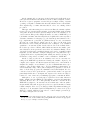
As a simple example, the formula φ given by ∀1 t. X(t) ↔ Y (s(t)) states
that every number in the set Y that is greater than 0 is the successor of a
number in the set X and vice versa. A WS1S interpretation for this formula can
be encoded by a string b(0)b(1) . . . b(m), where each b(i) is a letter in B2 . To
visualize this, we write letters (b1 , b2 ) vertically; the first track encoded in the
string determines an interpretation for X, and the second an interpretation for
Y . Two such interpretations for WS1S are
I1 =
X 101000
Y 110100
and I2 =
X 01000
.
Y 00000
The first interpretation, for example, interprets X as {0, 2} and Y as {0, 1, 3}.
φ is satisfied for WS1S in the first interpretation (i.e., it is a model of φ) and
not satisfied in the second, which we write as I1 |=WS1S φ and, respectively,
I2 6|=WS1S φ. The same applies to S1S, if the strings are infinitely extended with
0s. Interpreted over (bit) strings, φ says that Y is the string X right-shifted one
position, with the initial bit arbitrarily filled.
Tool support There are several implementations of decision procedures for
WS1S [6, 9]. These are based on the fact that WS1S captures precisely the regular languages: the language associated with each WS1S formula φ (i.e., the
set of all strings that encode a model) is regular, and vice versa. Hence, using
automata theoretic techniques, given a formula φ, the systems construct an automaton that recognizes the models of φ. A formula φ(X) is a tautology iff the
corresponding automaton accepts the universal language on Bn . To decide S1S
a similar procedure based on Büchi automata can be used.
The decision problem for both logics is non-elementary [8]. In the case of
WS1S, despite such a poor worst-case complexity, the implemented decision
procedures work surprisingly well on many non-trivial problems. In particular,
the MONA system has been highly optimized and can quickly process many large
formulae (e.g., formulae with hundreds of thousands of symbols). The system has
been used to formalize and reason about sequential hardware [4] and protocols
[6], where a finite string encodes values of signals or the evolution of the system
state over time. In contrast to WS1S, there is no satisfactory tool support for S1S
and due to technical difficulties (concerning minimization and complementation)
it seems unlikely that similarly effective tools are possible for this logic.
3
A Semantics of Core-BLIF
3.1
An S1S Semantics
In Section 2.1 we explained the informal “synchronous hardware” semantics for
Core-BLIF: Combinational gates switch without delay and latches load in the
current value of the input signal at every tick of the global system clock. This
semantics is equivalent to stating that latches delay the incoming signal for one
time unit, if we take the time between two clock ticks to be one time unit. As
this delay is the only time-relevant issue that must be modeled, the natural
numbers can serve as the set of time points, which can be modeled using firstorder variables in S1S. Further, since a signal in Core-BLIF is a binary valued
function of time, a signal can be modeled in S1S by a second-order variable, used
to formalize the set of time points at which the signal has the value 1.
We now define the semantics of Core-BLIF as a family of functions [[·]]NT
S1S ,
where each function maps the language associated with a non-terminal symbol
N T of the Core-BLIF abstract syntax (see Figure 1) to an S1S formula. The
semantics is summarized in Figure 3 and we describe below the main semantic
functions.3 Figure 4 gives the S1S formulae resulting from this translation for
the traffic lights example.
The function [[·]]model
translates a circuit into a predicate definition in S1S.4
S1S
This way of modeling circuits as predicates (semantically, relations) is standard
3
4
Note that in Figure 3, quantification over a list of variables represents quantification
over all members of the list.
Predicate definitions are not part of the monadic logics we defined. We can simply
view them as extra-logical definitions or macros. Our use of them has a practical
advantage: The MONA system supports predicate definitions and predicates are
compiled individually, only once, into automata. Hence, these definitions support not
only a compositional semantics, but also the hierarchical construction of automata.
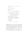
Types: (T is the set of S1S terms, cf. grammar in Section 2.2)
[[·]]model
: model → φ
S1S
[[·]]comp
: component → T → φ
S1S
[[·]]row
S1S
: row → identifier∗ → T → φ
[[·]]literal
: literal → identifier → T → φ
S1S
Definitions:
[[(name, Ins, Outs, Locals, [comp1 , . . . , compn ])]]model
=
S1S
Vn
2
1
name(Ins, Outs) ≡ ∃ Locals. i=1 ∀ t. [[compi ]]comp
S1S (t)
[[Comb(Ins, Outs, −, [(In1 , Out1 ), . . . , (Inn , Outn )])]]comp
S1S (t) =
Wn
row
row
i=1 ([[Ini ]]S1S (Ins)(t) ∧ [[Outi ]]S1S (Outs)(t))
[[Comb(Ins, Outs, default, [(In1 , Out1 ), . . . , (Inn , Outn )])]]comp
S1S (t) =
Wn
row
row
i=1 ([[Ini ]]S1S (Ins)(t) ∧ [[Outi ]]S1S (Outs)(t))
Vn
row
∨ i=1 ¬[[Ini ]]row
S1S (Ins)(t) ∧ [[default]]S1S (Outs)(t)
[[Latch(In, Out)]]comp
S1S (t) = In(t) ↔ Out(s(t))
[[Subckt(name, form act)]]comp
S1S (t) = name([form act])
comp
[[Reset(comb gate)]]comp
S1S (t) = [[Comb(comb gate)]]S1S (0)
V
n
literal
[[(lit1 , . . . , litn )]]row
S1S (Id1 , . . . , Idn )(t) =
i=1 [[liti ]]S1S (Idi )(t)
[[0]]literal
S1S (Id)(t) = ¬Id(t)
[[1]]literal
S1S (Id)(t) = Id(t)
[[−]]literal
S1S (Id)(t) = true
Fig. 3. The S1S semantics of Core-BLIF.
in higher-order logics [5]. A predicate describes a relation between input and
output signals. Components of the circuit are modeled as constraints on the
signals of the circuit and are conjoined together. Internal signals are hidden
by existential quantification, which asserts the existence of intermediate values,
consistent with the constraints. The formula that models the complete circuit
therefore states that all these constraints must be met at every time point. The
time point is an additional parameter for the semantics of component, row, and
literal; it can be any value of T , which denotes the set of all first-order S1S
terms given by the grammar in Section 2.2.
The function [[·]]comp
S1S is used to translate combinational gates, latches, and resets. Because combinational gates have no delay and no internal state, they can
be modeled as a relation that has to hold of the corresponding signals at each
ControlLogic(P resentSig, Button, N extSig) ≡
∀1 t. (P resentSig(t) ∧ Button(t) ∧ ¬N extSig(t)) ∨
(¬(P resentSig(t) ∧ Button(t)) ∧ N extSig(t))
Lights(Button, CarSig, P edestSig) ≡
∃2 T mp. ControlLogic(CarSig, Button, T mp, end) ∧
∀1 t. (T mp(t) ↔ CarSig(s(t))) ∧
∀1 t. (¬CarSig(t) ∧ P edestSig(t)) ∨
(CarSig(t) ∧ ¬P edestSig(t))
Fig. 4. The S1S translation of the traffic light example from section 2.1.
time point. If no default output is given, this relation is simply the disjunction
of the row pairs in the table; otherwise the relation additionally contains each
input pattern that is not covered by the table together with the default value
for the outputs. For the translation of rows and literals, the names of the respective signals are additional parameters of the semantic functions. Latches, as
mentioned previously, delay the input by one time unit. The initial value can
be given by a reset table. Syntactically and semantically, reset tables are like
combinational gates, except that they formalize a relation over just the initial
time point.
3.2
Restriction to WS1S
The above translation models Core-BLIF circuit descriptions by modeling the
evolution of the system state over infinitely many time points. Although this
is a simple, appealing, semantics, the lack of tool support for S1S means we
cannot directly use it for automated reasoning. In this section we show how the
semantics can be recast in WS1S, whereby we can automate reasoning using the
MONA system.
Modeling infinite behavior is not generally possible in WS1S since all sets
are finite and hence any signal modeled must constantly take the value 0 after
some time point. However, for verifying safety properties it is sufficient to model
all the finite prefixes of a circuit’s behavior, which we can do by modeling its
behavior from time 0 up to some point end, which is finite, but unbounded.
We do this as follows. We formalize end as a first-order variable in WS1S,
given as an additional parameter to every predicate. As explained previously,
components are modeled in S1S by constraints on the signals that have to be
met at every time point. We now restrict this use of universal first-order quantification to time points up to end (so the values of the signal after end are not
constrained). For latches we restrict the universal quantification to time points
[[(name, Ins, Outs, Locals, [comp1 , . . . , compn ])]]model
WS1S =
Vn
2
1
name(Ins, Outs, end) ≡ ∃ Locals. i=1 ∀ t ≤ end. [[compi ]]comp
WS1S (t)
[[Latch(In, Out)]]comp
WS1S (t) = t < end → (In(t) ↔ Out(s(t)))
[[Subckt(name, form act)]]comp
WS1S (t) = name([form act], end)
Fig. 5. The modifications of the semantics necessary for WS1S
strictly before end since this constrains all successive time points up to end in the
output signal. We summarize these modifications to the semantics in Figure 5
and give the WS1S translation of the traffic light example in Figure 6.
This restriction of the S1S semantics to finite interpretations is sensible.
Under our translations, an infinite string is a model of the S1S semantics of a
BLIF-MV circuit C iff all finite non-empty prefixes of the string are models of
the WS1S semantics of C. We sketch the reasons for this below.
Proof Sketch. Observe that, since we do not constrain the time points after
end, two finite interpretations of the signals of C are equivalent, if they are equal
up to end. Hence, we introduce the following notation: For a formula φ, with
free second-order variables X = (X1 , . . . , Xn ) and a first-order variable end, we
say w ∈ ({0, 1}n )+ models φ in the WS1S semantics, relative to end, written
w |≡WS1S φ, iff w encodes a model for φ, where Xi is interpreted as the ith track
of w and end is interpreted as |w| − 1.
Now let pre(w) be the finite non-empty prefixes of w. Formally we will show
that w|=S1S [[C]]S1S iff for all w0 ∈ pre(w), w0 |≡WS1S [[C]]WS1S .
To begin with, the (W)S1S translation of a circuit C can be rewritten into
the form
[[C]]S1S (X) ≡ ∃2 L. ∀1 t. φ(X, L, t)
[[C]]WS1S (X, end) ≡ ∃2 L. ∀1 t ≤ end. φ(X, L, t) ,
where L represents the local signals of the overall circuit and φ is a quantifier-free
formula that accesses only the signals at time points 0, t − 1, and t.
The left-to-right direction of the claim is straightforward. For the converse,
assume we are given an infinite word w such that all non-empty finite prefixes
satisfy [[C]]WS1S relative to end. We have to show w|=S1S [[C]]S1S . If there are no
local signals, this is also straightforward by induction on the structure of the
components. Otherwise, for every w0 ∈ pre(w) there is an instance of L where φ
is satisfied for all points up to the last position of w0 . Let N ⊆ ({0, 1}|L| )∗ be the
set that contains all such instances for L and, additionally, contains the empty
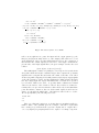
word. Let E be the relation (u, v) ∈ E iff u·x = v for some x ∈ {0, 1}|L| . (Figure 7
shows the graph for the example φ(L, end) ≡ ∀1 t. ( t > 0 ∧ t ≤ end ) → ¬L(t−1).)
ControlLogic(P resentSig, Button, N extSig, end) ≡
∀1 t ≤ end. (P resentSig(t) ∧ Button(t) ∧ ¬N extSig(t)) ∨
(¬(P resentSig(t) ∧ Button(t)) ∧ N extSig(t))
Lights(Button, CarSig, P edestSig, end) ≡
∃2 T mp. ControlLogic(CarSig, Button, T mp, end) ∧
∀1 t < end. (T mp(t) ↔ CarSig(s(t))) ∧
∀1 t ≤ end. (¬ CarSig(t) ∧ P edestSig(t)) ∨
(CarSig(t) ∧ ¬P edestSig(t))
Fig. 6. The WS1S translation of the traffic light example from Section 2.1.
From the fact that N is prefix-closed, it follows that the graph (N, E) is a
tree (with the empty word as root). Moreover it is finitely branching (since the
alphabet is finite) and for every depth there must be at least one node at this
depth (since for every prefix of w there is a satisfying instance for L of the same
length). From König’s lemma the tree must contain an infinite path, i.e. there
must be an infinite string S, such that all strings on the path are finite prefixes
of S. Thus S satisfies the constraints given by φ for all points up to an arbitrary
bound end and, relying on the case without local signals, we can conclude that
it does so for all points. Hence w|=S1S [[C]]S1S .
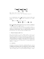
t
u
Unfortunately, for certain kinds of circuit descriptions, the WS1S semantics
allows more models than intended: if a string encodes a model under the WS1S
semantics of the circuit up to end, it is not always the case that this is a prefix
of a string under the S1S semantics. Consider the following example:
.names K L
0 0
0 1
.latch L K
This has exactly one model in the S1S semantics: K and L are constantly 0.
However, in the WS1S semantics, for end = 0 (i.e., the string of length 1), we
also have the model K(0) = 0 and L(0) = 1. The problem is that combinational
tables define relations that need not be total on the input side, i.e. the gate
can “refuse” certain inputs. Hence, a behavior that is consistent with the circuit
description up to a given time point can later be “ruled out”. The graph of all
models of this circuit, if we consider L as output, is the same as in Figure 7. The
undesired models are those that are not on an infinitely long path and therefore
cannot be extended arbitrarily far.
To eliminate these undesired models, we add to our specification the constraint that a finite behavior is only allowed if it can be extended beyond end
ε
0
0
1
0
00
1
1
0
000
...
1
01
001
Fig. 7. Graph of finite models of the language
φ(L, end) ≡ ∀1 t. ( t > 0 ∧ t ≤ end) → ¬L(t − 1), including the empty word.
up to an arbitrary time point new end such that the extension is still a valid
behavior of the circuit up to new end. It turns out that this is easy to formalize
in WS1S:
C 0 (X, end) ≡ C(X, end) ∧ ∀1 new end > end.
∃2 Y . C(Y , new end) ∧ ∀1 t ≤ end. X(t) ↔ Y (t) .
Here C is the WS1S semantics (as defined above) of a circuit over the list of
signals X. The models of C 0 , relative to end, now have the property that they
are precisely the prefixes of infinite behaviors.
As a consequence of the relation between the S1S and WS1S semantics of a
circuit, we can check safety properties (as defined in [1]) with respect to the S1S
semantics by checking them with respect to our WS1S translation: if MONA
responds that no safety violation occurs in any finite prefix of the behavior of
the circuit, then we can conclude the same for the infinite behavior.
4
Formal Analysis with MONA
Given a system description, we can use our B2M compiler to produce a set of
formulae that express the semantics of the description’s components in WS1S,
in the syntax of MONA. We can then use MONA directly for simulation or for
verification with respect to properties also expressed in WS1S. We now provide
examples that illustrate the flexibility we gain by using a purely logical approach:
by expressing appropriate constraints, we can restrict the set of possible circuit
behaviors to the cases of interest; in this way there is a seamless transition from
simulation to verification.
4.1
Simulation
As mentioned in Section 2.2, the models of a WS1S formula can be encoded
by strings in a regular language. Given a formula, MONA computes a minimal
deterministic finite automaton that accepts exactly the models of the formula
and, from this automaton, MONA extracts minimal strings that are in, and
outside, the language (if there are any). The strings in the language constitute
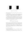
Button 0 0 0 0 0 x
Button 0 1 0 1 0 1
Car
011111
Car
010101
P ed
100000
P ed
101010
end
000001
end
000001
(b) Button pressed every other time unit
(a) Run of length 5
Fig. 8. Runs of the traffic light
simulated runs. The automaton generated constitutes a finite representation of
all possible behaviors.
It is a simple matter to express, logically, constraints on the runs one is interested in. One can specify, for instance, runs of some particular length, or by
expressing constraints on some of the input variables, and existentially quantifying over them, one can simulate outputs in response to certain inputs.
A simulation of the lights for, say, the time interval from 0 to 5 can be
obtained using MONA by the formula Lights(Button, Car, P ed, 5), which yields
the run shown in Figure 8(a). Here x stands for an arbitrary Boolean value. This
run corresponds to a situation in which the button is not pressed during the first
five time units. If we desire, we can further restrict the circuit by providing more
constraints on the input signals. For instance, to simulate the cases where the
button is pressed every other time unit, we can specify
Lights(Button, Car, P ed, end) ∧ end = 5
∧∀1 t < end. Button(t) ↔ ¬Button(s(t)) .
In this case, MONA responds with the simulated run shown in Figure 8(b). The
fact that we can specify arbitrary WS1S constraints on both inputs and outputs
and get a minimal automaton for the set of behaviors consistent with these
constraints makes our approach to simulation quite flexible. For instance, if one
has discovered some non-intended behavior, one can easily specify the property
of the outputs that is violated and obtain the set of inputs that can cause this
bug. Indeed, one can even stipulate the existence of some undesired behavior
and generate a run for it.
4.2
Equivalence Checking
We can also use MONA to check equivalence of a given hardware description
with some other sequential system.
To illustrate this, we have developed a slightly more sophisticated variant of
the traffic light example, called PhaseLight: a new phase of the light, i.e. a time
point where a light can change, is now controlled by an additional timer. When
the pedestrians see red, the control logic stores, in an additional one bit register,
whether the button was pressed at least once during this phase. We omit giving
here the straightforward BLIF-MV description of PhaseLight.
We can now show, for example, that the simple traffic light circuit is a special
case of the new circuit. Namely, if T imer is constantly 1, both circuits are
equivalent.
Lights(Button, Car, P ed, end) ↔
(∃2 T imer. ∀1 t ≤ end. T imer(t) ∧ PhaseLight(T imer, Button, Car, P ed, end))
MONA can verify such formulae in negligible time and provides a counterexample (i.e. a string not in the language) in invalid cases.
4.3
Safety properties
By reasoning about the finite traces of our systems, we can establish safety
properties. For our light example, we can show, for example, that:
(P1) The lights cannot simultaneous be green (or red) for the cars and pedestrians.
(P2) If the cars’ light is red, it turns green in the next phase.
(P3) If the pedestrian’s light is red and they press the button, then their light
turns green in the next phase.
Note that (P2) and (P3) state eventualities, but since we stipulate when they
must occur, they are indeed formalizable in WS1S.
The formalization of (P1)–(P3) is given in Figure 9: the lights are correct
iff every assignment for the signals and end that constitutes a possible behavior
of the PhaseLight circuit also satisfies the properties. For brevity, we define a
predicate NextPhase, which states that, from time point t on, t0 is the next rise
of the timer signal plus one time unit. This unit delay is needed since there is a
latch between inputs and outputs that delays the reaction of the control logic.
(P2) for instance is formulated as follows: for arbitrary time points t and t0 up
to end, if the cars’ light is red at time t and t0 is the next phase after t, then
the cars’ light is green at t0 . (Recall that red is encoded as 0 and green as 1 and
t0 ≤ end is contained in NextPhase). Again MONA verifies this automatically,
requiring negligible time.
4.4
Performance
By using a general logic and a general purpose decision procedure we pay a performance price over more specialized algorithms for automata synthesis. However, for many examples of interest we get acceptable running times, which are
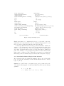
typically around one order of magnitude slower then the running times of the
NextPhase(T imer, t, t0 , end) ≡
t < t0 ∧ t0 ≤ end ∧ T imer(t0 − 1) ∧
∀1 t00 . ((t ≤ t00 ∧ t00 < t0 − 1) → ¬ T imer(t00 ))
LightsCorrect(Button, T imer, Car, P ed, end) ≡
PhaseLight(Button, T imer, Car, P ed, end) →
∀1 t ≤ end. ((Car(t) ↔ ¬P ed(t)) ∧
(∀1 t0 . ((¬Car(t) ∧ NextPhase(T imer, t, t0 , end)) → Car(t0 ))) ∧
(∀1 t0 . ((¬P ed(t) ∧ Button(t) ∧ NextPhase(T imer, t, t0 , end)) → P ed(t0 ))))
Fig. 9. The formulation of the properties of the traffic light example in WS1S
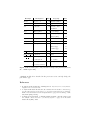
VIS system. In Figure 10 we summarize the times for those circuits of the VIS
example suite [13] that can be handled using our compiler and MONA without
exceeding the physical memory5 .
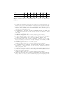
Although run-times and example coverage are worse in our setting, we believe that substantial improvements are possible through compiler optimizations.
Namely, the performance of MONA is quite sensitive to issues such as quantifier
scoping and the way (equivalent) formulae are expressed. To gain some insights
we compared the verification performance of compiler generated versus hand
optimized MONA formulae. As an example, we verified the correctness of the
sequential n-bit von Neumann adder for different values of n (by comparing results with a standard carry-chain adder). The hand optimizations included better
quantifier scoping, constraint propagation and simplifications for combinational
parts of the circuits. The times in Figure 11 show that there is considerable room
for improvement, though there seems to be a general size frontier for the circuits
that can be represented by MONA.
5
Conclusions
We have defined two formal semantics for BLIF-MV using the monadic logics
S1S and WS1S. These provide precise, unambiguous interpretations over finite
and infinite time intervals, and the WS1S semantics can directly be used for
different kinds of symbolic analysis with the MONA system.
Our compiler provides a simple but flexible tool for understanding and experimenting with BLIF-MV specifications. However, the use of a simple highlevel semantics and a general tool partially conflicts with the goal of optimal
performance. As future work, we intend to investigate to what extent compiler
5
Running times are for a Ultra Sparc 2 450MHz workstation with 2,25 GB memory,
typical memory usage for the examples was between 1 and 50 MB.
Example
Description
arbiter
Bus protocol
counter
3 Bit
crd
Crossroads
Size
Property
Time
10 Mutual exclusion
1
1 Approx. Liveness
<1
19 Self test const. 1
1
and Mutex
ctlp3
3 Philosophers
6 Reader unique
1
dcnew
Train-crossing
38 Safety1 (False)
38
Safety2 (True)
32
8 Queens
Setting valid?
31 Exists valid setting
exampleS
req/ack-module
19 req until ack
mult 6x6
4 multipliers
ping pong
Simple game
190
4
each 4 First two equivalent
84
Third buggy
85
Fourth buggy
85
6 Safety
<1
ping pong new ... extension
7 Safety
<1
tbl one bug
1 Equivalence of
<1
Shows bug in
the VIS system
tlc
Traffic light controller
two circuits
13 Safety/Eventualities
<1
by Conway & Mead
Fig. 10. Verification times (in seconds) of standard examples using MONA (size means
size of BLIF input in KB).
optimizations, like those sketched in the previous section, can help bridge the
performance gap.
References
1. B. Alpern and F. B. Schneider. Defining liveness. Information Processing Letters,
21(4):181–185, 7 October 1985.
2. A. Ayari and D. Basin. Bounded model construction for monadic second-order logics. In 12th International Conference on Computer-Aided Verification (CAV’00),
number 1855 in Lecture Notes in Computer Science, pages 99–113, Chicago, USA,
July 2000. Springer-Verlag.
3. D. Basin and S. Friedrich. Combining WS1S and HOL. In D.M. Gabbay and
M. de Rijke, editors, Frontiers of Combining Systems 2, pages 39–56. Research
Studies Press/Wiley, 2000.
n Bit
4
5
6
Compiler-generated
17
211
∞
Hand optimized
<1
<1
1
7
8
9
10
11
6
22
74
239
∞
Fig. 11. Verification times for von Neumann adder; ∞ denotes exceeding memory
resources.
4. D. Basin and N. Klarlund. Automata based symbolic reasoning in hardware verification. The Journal of Formal Methods in Systems Design, 13(3):255–288, 1998.
5. M. Gordon. Why higher-order logic is a good formalism for specifying and verifying
hardware. In G. J. Milne and P. A. Subrahmanyam, editors, Formal Aspects of
VLSI Design. North-Holland, 1986.
6. J.G. Henriksen, J. Jensen, M. Jørgensen, N. Klarlund, B. Paige, T. Rauhe, and
A. Sandholm. Mona: Monadic second-order logic in practice. In TACAS ’95, LNCS
1019, 1996.
7. Y. Kukimoto. BLIF–MV. 1996.
Availlable at http://www-cad.eecs.berkeley.edu/Respep/Research/vis/.
8. A. Meyer. Weak monadic second-order theory of one successor is not elementaryrecursive. In LOGCOLLOQ: Logic Colloquium. LNM 453, Springer, 1975.
9. F. Morawietz and T. Cornell. On the recognizibility of relations over a tree definable in a monadic second-order tree description language. Research Report SFB
340-Report 85, 1997.
10. A methodology for verification of real–time systems.
Availlable at http://www-cad.eecs.berkeley.edu/Respep/Research/hsis/.
11. J. W. Thatcher and J. B. Wright. Generalized finite automata theory with an
application to a decision problem of second-order logic. Mathematical Systems
Theory, 2(1):57–81, 1967.
12. W. Thomas. Automata on infinite objects. In J. van Leeuwen, editor, Handbook
of Theoretical Computer Science, volume B, chapter 4. MIT Press/Elsevier, 1990.
13. VIS Group. VIS user’s manual.
Availlable at http://www-cad.eecs.berkeley.edu/Respep/Research/vis/.
14. VIS Group. VIS: A system for Verification and Synthesis. In R. Alur and T. Henzinger, editors, Proceedings of CAV ’96, LNCS 1102, pages 428–432. Springer, 1996.