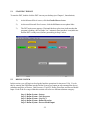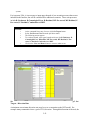
1
United States
Environmental Protection
Agency
Office of Research and
Development
Washington, DC 20460
EPA/R-99/XXXX
December 2000
www.epa.gov
A Decision Support Tool for
Assessing the Cost and
Environmental Burdens of
Integrated Municipal Solid Waste
Management Strategies:
USERS MANUAL
DRAFT
EPA/XXX-R-99-XXX
December 2000
A Decision Support Tool for Assessing
the Cost and Environmental
Performance of Integrated Municipal
Solid Waste Management Strategies:
USERS MANUAL
Prepared By:
Research Triangle Institute
Center for Environmental Analysis
3040 Cornwallis Road
Research Triangle Park, NC 27709
with
North Carolina State University
Department of Civil Engineering
Mann Hall - Stinson Dr.
Raleigh, NC 27695
U.S. Environmental Protection Agency
Cincinnati, OH
Prepared For:
Susan Thorneloe
National Risk Management Research Laboratory
Air Pollution Prevention and Control Division (MD-63)
U.S. Environmental Protection Agency
Research Triangle Park, NC 27711
Notice
This manual has been developed as part of research funded by the U.S. Environmental Protection
Agency and U.S. Department of Energy through EPA Cooperative Agreement No. CR823052
with the Research Triangle Institute. The decision support tool is intended for use in evaluating
the relative cost and environmental burdens of integrated municipal solid waste management
strategies. The information and results from this tool are not intended for use in making
comparative assertions about the environmental preferability of alternative materials or products.
Use of the methods or data presented in this manual does not constitute endorsement or
recommendation for use. This manual is subject to review and modification prior to conclusion
of the research. Mention of trade names or commercial products does not constitute
endorsement or recommendation.
iii
Abstract
Communities throughout the United States are struggling to develop efficient and cost-effective
plans for managing their municipal solid waste (MSW). Today's MSW management systems
often are complex and highly integrated systems that might include separate recyclables
collection, recovery, composting, combustion, and disposal. Communities now must make
complex decisions requiring an analysis of both cost and environmental burdens for these
integrated systems. Despite the movement toward integrated systems, many of the existing
techniques for analyzing the environmental and economic performance of MSW management
systems focuses on the individual operations in isolation rather than as part of an integrated
system.
To properly account for all of the environmental effects associated with integrated MSW
management systems, planners must have tools that allow them to examine factors outside of the
traditional MSW management framework of activities occurring from the point of waste
collection to final disposal. The U.S. Environmental Protection Agency's (EPA’s) Office of
Research and Development, Air Pollution Prevention and Control Division, with cofunding from
the U.S. Department of Energy, worked with solid waste management and life cycle assessment
(LCA) experts from Research Triangle Institute, North Carolina State University, the University
of Wisconsin-Madison, Franklin Associates, and Roy F. Weston to develop a computer based a
tool to assist solid waste practitioners in identifying integrated MSW management strategies that
minimize both cost and environmental burdens.
This user’s manual has been prepared to provide the reader with a general overview of the
computer tool developed through this research as well as more detailed information to assist
users in building scenarios for analysis. Detailed documentation about the data and methods
used for each unit process included in the tool are available as separate documents.
iv
Table of Contents
Notice . . . . . . . . . . . . . . . . . . . . . . . . . . . . . . . . . . . . . . . . . . . . . . . . . . . . . . . . . . . . . . . . . . . . . . ii
Abstract . . . . . . . . . . . . . . . . . . . . . . . . . . . . . . . . . . . . . . . . . . . . . . . . . . . . . . . . . . . . . . . . . . . . iii
List of Figures . . . . . . . . . . . . . . . . . . . . . . . . . . . . . . . . . . . . . . . . . . . . . . . . . . . . . . . . . . . . . . . . v
List of Tables . . . . . . . . . . . . . . . . . . . . . . . . . . . . . . . . . . . . . . . . . . . . . . . . . . . . . . . . . . . . . . . . vi
Abbreviations and Symbols . . . . . . . . . . . . . . . . . . . . . . . . . . . . . . . . . . . . . . . . . . . . . . . . . . . . vii
Key Terms and Definitions . . . . . . . . . . . . . . . . . . . . . . . . . . . . . . . . . . . . . . . . . . . . . . . . . . . . viii
Section 1
Introduction . . . . . . . . . . . . . . . . . . . . . . . . . . . . . . . . . . . . . . . . . . . . . . . . . . . .
1.1
What are Appropriate Uses for the Tool? . . . . . . . . . . . . . . . . . . . . . . .
1.2
What are the Basic Components of the Tool? . . . . . . . . . . . . . . . . . . . .
1.3
What are the Hardware and Software Requirements? . . . . . . . . . . . . . .
1.4
How Do I Get the Tool? . . . . . . . . . . . . . . . . . . . . . . . . . . . . . . . . . . . .
1.5
Is the Tool Complicated to Use? . . . . . . . . . . . . . . . . . . . . . . . . . . . . . .
1.6
How Can I Get Assistance on Using the Tool? . . . . . . . . . . . . . . . . . . .
1.7
What Type of Input Data Will I Need to Run the Tool? . . . . . . . . . . . .
1.8
Organization of this Users Manual . . . . . . . . . . . . . . . . . . . . . . . . . . . .
Section 2
System Definition . . . . . . . . . . . . . . . . . . . . . . . . . . . . . . . . . . . . . . . . . . . . . . . 2-1
2.1
System Boundaries . . . . . . . . . . . . . . . . . . . . . . . . . . . . . . . . . . . . . . . . . 2-1
2.1.1 General Boundaries for LCI . . . . . . . . . . . . . . . . . . . . . . . . . . . 2-4
2.1.2 General Boundaries for Cost Analysis . . . . . . . . . . . . . . . . . . . . 2-4
2.2
Waste Generation . . . . . . . . . . . . . . . . . . . . . . . . . . . . . . . . . . . . . . . . . . 2-5
2.2.1 Source Reduction . . . . . . . . . . . . . . . . . . . . . . . . . . . . . . . . . . . . 2-6
2.2.2 Backyard Composting . . . . . . . . . . . . . . . . . . . . . . . . . . . . . . . . 2-7
2.2.3 In-Home Recyclables Washing and Separation . . . . . . . . . . . . . 2-7
2.3
Waste Composition . . . . . . . . . . . . . . . . . . . . . . . . . . . . . . . . . . . . . . . . 2-7
2.4
Waste Management Processes . . . . . . . . . . . . . . . . . . . . . . . . . . . . . . . . 2-9
2.5
Additional System Processes . . . . . . . . . . . . . . . . . . . . . . . . . . . . . . . . 2-11
2.6
Data Parameters Tracked . . . . . . . . . . . . . . . . . . . . . . . . . . . . . . . . . . . 2-11
v
1-1
1-1
1-2
1-4
1-4
1-5
1-5
1-5
1-6
Table of Contents (Cont.)
Section 3
Process Models Descriptions . . . . . . . . . . . . . . . . . . . . . . . . . . . . . . . . . . . . . . . 3-1
3.1
Collection . . . . . . . . . . . . . . . . . . . . . . . . . . . . . . . . . . . . . . . . . . . . . . . . 3-1
3.2
Transfer Station . . . . . . . . . . . . . . . . . . . . . . . . . . . . . . . . . . . . . . . . . . . 3-7
3.4
Mixed and Yard Waste Composting . . . . . . . . . . . . . . . . . . . . . . . . . . 3-11
3.5
Combustion . . . . . . . . . . . . . . . . . . . . . . . . . . . . . . . . . . . . . . . . . . . . . 3-16
3.6
Refuse Derived Fuel and Processed Refuse Fuel . . . . . . . . . . . . . . . . 3-19
3.7
Landfill . . . . . . . . . . . . . . . . . . . . . . . . . . . . . . . . . . . . . . . . . . . . . . . . . 3-25
3.8
Electrical Energy . . . . . . . . . . . . . . . . . . . . . . . . . . . . . . . . . . . . . . . . . 3-28
3.9
Mixed and Yard Waste Composting . . . . . . . . . . . . . . . . . . . . . . . . . . 3-32
3.10 Remanufacturing . . . . . . . . . . . . . . . . . . . . . . . . . . . . . . . . . . . . . . . . . 3-34
Section 4
Model Capabilities, Uses, and Limitations . . . . . . . . . . . . . . . . . . . . . . . . . . . . 4-1
4.1
General Model Uses and Limitations . . . . . . . . . . . . . . . . . . . . . . . . . . 4-1
4.2
Limitations Associated With The Process Models . . . . . . . . . . . . . . . . 4-8
4.3
Additional Considerations . . . . . . . . . . . . . . . . . . . . . . . . . . . . . . . . . . 4-10
Section 5
Scenario Building Using The Tool . . . . . . . . . . . . . . . . . . . . . . . . . . . . . . . . . . . 38
5.1
Recommended Steps for Scenario Building . . . . . . . . . . . . . . . . . . . . 4-10
APPENDIX
A:
Example Case Study
APPENDIX
B:
FAQs
APPENDIX
C:
Trouble Shooting
APPENDIX
D:
Available Supporting Documentation
vi
List of Figures
Figures
1-1
2-2
2-2
Page
Conceptual Framework for the Decision Support Tool . . . . . . . . . . . . . . . . . . . . . . . . . 1-3
Overall System . . . . . . . . . . . . . . . . . . . . . . . . . . . . . . . . . . . . . . . . . . . . . . . . . . . . . . . . 2-2
Example System Flow for Newsprint . . . . . . . . . . . . . . . . . . . . . . . . . . . . . . . . . . . . . . 2-3
List of Tables
Table
Page
2-1
Components of MSW Considered in the System . . . . . . . . . . . . . . . . . . . . . . . . . . . . . 2-8
3-1
Electric Region Definitions . . . . . . . . . . . . . . . . . . . . . . . . . . . . . . . . . . . . . . . . . . . . . 3-30
3-2
Electric Region Locations . . . . . . . . . . . . . . . . . . . . . . . . . . . . . . . . . . . . . . . . . . . . . . 3-30
vii
Abbreviations and Symbols
BTU
U.S. DOE
DQG
DQI
DST
EIA
FAL
GUI
KWH
LCA
LCI
MRF
MSW
NCSU
NERC
O&M
POTW
RCRA
RDF
RTI
SETAC
TPD
U.S. EPA
UW
WTE
British Thermal Unit
United States Department of Energy
Data Quality Goal
Data Quality Indicator
Decision Support Tool
Energy Information Administration
Franklin Associates, Limited
Graphical User Interface
Kilowatt Hour
Life-Cycle Assessment
Life-Cycle Inventory
Materials Recovery Facility
Municipal Solid Waste
North Carolina State University
North American Electric Reliability Council
Operation and Maintenance
Publicly Owned Treatment Works
Resource Conservation and Recovery Act
Refuse-Derived Fuel
Research Triangle Institute
Society for Environmental Toxicology and Chemistry
Tons Per Day
United States Environmental Protection Agency
University of Wisconsin - Madison
Waste-To-Energy Combustion
viii
Key Terms and Definitions
Allocation: Technique for partitioning multiple inputs and outputs from a system.
Cost: Amount actually incurred for the provision of a product or service. Cost can include
internal cost accrued by an organization, external costs accrued by society.
Data Quality Indicator: Measure which characterizes an attribute(s) of data or data sets.
Function: Performance characteristic of a system.
Functional Unit: Measure of performance of the main functional output of a system.
Integrated Waste Management: Interlinked stages of a system to collect, process, treat, and
dispose of waste.
Life Cycle: Consecutive and interlinked stages of a system that extend from raw materials
acquisition or generation of natural resources to final disposal.
Life Cycle Assessment: Compilation and evaluation, according to a systematic set of
procedures, of the inputs and outputs of materials and energy and the associated environmental
impacts directly attributable to the function of a product throughout its life cycle.
Life Cycle Impact Assessment: Phase of life cycle assessment aimed at understanding and
evaluating the magnitude and significance of environmental impacts based on a life cycle
inventory analysis.
Life Cycle Inventory Analysis: Phase of life cycle assessment that involves compiling and
quantifying the inputs and outputs for a given product system throughout its life cycle.
Municipal Solid Waste: Waste generated in the residential, multifamily, and commercial
sectors. Includes durable goods, nondurable goods, containers and packaging, food waste, and
yard trimmings. Also includes ash from waste combustion. Excludes industrial process waste,
sludge, construction and demolition waste, pathological waste, agricultural waste, mining waste
and hazardous waste.
Price: Amount actually charged/paid for a product or service.
ix
Key Terms and Definitions (Cont.)
Process Model: Mathematical representation of a unit process to calculate cost and
environmental burdens as a function of the quantity and composition of the waste or material
processed.
Raw Material: Primary or secondary recovered or recycled material that is used in a system to
produce a product.
System: Collection of unit processes which, when acting together, perform some defined
function.
Unit Process: Component of the system being studied that is a collection of operations which
transforms inputs into outputs, such as manufacturing, waste collection, materials recovery, etc.
Section 1
Introduction
This manual is designed to provide the user of the Decision Support Tool (DST) with the
essential information required to use the tool to conduct scenario analyses of integrated
municipal solid waste (MSW) management strategies. The overall focus of the DST is to
support the evaluation of cost and environmental burdens associated with alternative strategies
for integrated MSW management in a particular community or region.
The tool is designed to analyze the management of MSW of a given quantity and composition.
It considers all activities required to manage the MSW from the time it is sent out for collection
to its ultimate disposition, whether that be disposal in a landfill, compost applied to the land,
energy recovered from combustion or landfills, or materials recovered and remanufactured into
new products. It can help to answer questions such as how do the cost and environmental
burdens associated with a MSW management system change if clear glass containers are added
to or removed from a community’s recycling program? Or, what are the tradeoffs in cost and
environmental burdens if newspaper is recycled versus combusted or landfilled with energy
recovery?
This user’s manual will first answer some basic questions and, in subsequent chapters, will
summarize the methodologies used in the tool and demonstrate how to use it to conduct scenario
analyses of integrated MSW management options. Upon accessing the DST, you’ll find the help
system especially helpful. To access the help system, simply press the help button on any screen
or from the menu.
1.1
WHAT ARE APPROPRIATE USES FOR THE TOOL?
The DST is a screening level tool designed for use in evaluating community level MSW
management strategies. It allows you to conduct scenario analyses of strategies with the
objective of optimizing cost or environmental performance of the system. The MSW
management system modeled may be an existing system, entirely new systems, or some
combination of both based on user-specified data on MSW generation, requirements, etc. The
processes that can be modeled include waste generation, collection, transfer, separation (material
recovery and drop-off facilities), composting, combustion, refuse-derived fuel, and disposal in a
landfill. Existing facilities and equipment can be incorporated as model constraints to ensure
that previous capital expenditures are not negated by the model solution.
The DST was designed with local governments and solid waste planners in mind as the primary
users of the tool. At the local level, the tool can be used to evaluate, for example, the affects of
1-1
changes in the existing MSW management on cost and environmental burdens, identify least cost
ways to manage recycling and waste diversion, evaluate options for reducing greenhouse gases
or air toxics, or estimate the environmental benefit of recycling. The tool will also be of value to
other user groups such as Federal agencies, environmental and solid waste consultants, industry,
LCA practitioners, and environmental advocacy organizations. These users can use the tool, for
example, to evaluate recycling policies and programs, policies and technologies for reducing
environmental burdens, and strategies for optimizing energy recovery from MSW.
The tool is not a cash flow model and therefore should not be used to set prices for any specific
waste management service. The cost results provided by the tool represent screening level
engineering costs. A more detailed cash flow analysis would be need to determine the
appropriate prices for services and materials.
The tool also should not be used to conduct life cycle comparisons of specific products or
materials. The LCI results for recycling are based on generic process designs for product
manufacturing and remanufacturing operations. To properly compare the preferability of
packaging materials, you would need to do a more in-depth analysis of the production, use, and
pre-consumer recycling of the products or materials.
Future information about the appropriate uses and limitations of the DST is provided in Section
4 of this users manual.
1.2
WHAT ARE THE BASIC COMPONENTS OF THE TOOL?
As illustrated in Figure 1-1, the DST consists of four basic components: process models, waste
flow model, optimization model, and a graphic user interface (GUI). The process models consist
of a set of spreadsheets developed in Microsoft Excel. These spreadsheets use a combination of
default and user supplied data to calculate the cost and life cycle inventory (LCI) coefficients on
a per unit mass basis for each of the 48 MSW components being modeled for each solid waste
management unit process (collection, transfer, etc.). For example, in the electric energy
spreadsheet, the user is asked to specify the fuel mix used to generate electricity in the
geographic region of interest. Based on this design information and the emissions associated
with generating electricity from each fuel type, the spreadsheet calculates coefficients for
emissions related to the use of a kilowatt hour of electricity. These emissions are then assigned
to waste stream components for each facility that uses electricity and through which the mass
flows. For example, material recovery facilities (MRFs) use electricity for conveyors and
lighting. The emissions associated with electricity generation would be assigned to the mass that
flowed through that facility. The user can bypass default data if more site specific data are
available.
1-2
Figure 1-1. Conceptual Framework for Decision Support Tool
The waste flow model essentially provides a mass balance of the system. MSW can be collected
by a variety of different collection alternatives and collection combinations and then can flow
through additional alternatives for transfer, separation, treatment, and disposal. The waste flow
model defines all possible pathways for the MSW. It helps to link the process models and
facilitate optimization. It also helps to prevent infeasible waste flows. For example, aluminum
cans would not go to a yard waste compost facility. Similarly, glass would not be collected and
sent to a MRF if the MRF doesn’t have a glass crusher. The waste flow model communicates
with the optimization module to search for optimal solutions from the large number of possible
MSW management strategies.
The optimization module is implemented using the CPLEX linear programming solver. The
model is constrained by mass flow equations that are based on the quantity and composition of
waste entering each unit process, and that intricately link the different unit processes in the waste
management system (i.e., collection, recycling, treatment, and disposal options). These mass
flow constraints preclude impossible or nonsensical model solutions. For example, these mass
flow constraints will exclude the possibility of removing aluminum from the waste stream via a
mixed waste MRF and then sending the recovered aluminum to a landfill. The user can identify
1-3
the objective as minimizing total cost or life-cycle parameter (e.g., energy consumption, carbon
equivalents, CO, CO2, NOx, particulate matter, and SOx). The optimization module uses linear
programming techniques to determine the optimum solution consistent with the user-specified
objective and mass flow, and user-specified constraints. Examples of user-specified constraints
are the use of existing equipment/facilities, and a minimum recycling percentage requirement.
The GUI consists of Microsoft Visual Basic routines that act to pull all components of the model
together to allow easy user manipulation of the spreadsheet models and the optimization module.
It allows additional user constraints to be specified and provides a graphical representation of the
solid waste management alternatives resulting from the optimization. Results are presented on a
cost or pounds of emission per ton basis and can be viewed at the system level, unit process
level, or MSW component level.
1.3
WHAT ARE THE HARDWARE AND SOFTWARE REQUIREMENTS?
The DST is a large and complex model that requires a high end computer and some special
software to run properly. This section describes the recommended hardware and software needs
for running the DST.
Hardware
To adequately run the DST, users will need a Pentium II PC compatible machine with at least a
16 gigabyte hard drive, 512 of RAM, 400MZ processor, and preferably a 17 inch color monitor.
Machines with less memory or processing capacity may be used but will result in slower run
times for the DST.
Software
Users will need Microsoft Office 97 and a license for a commercial software package called
Cplex to run the DST. Microsoft Office 97 is a standard software package. Cplex is a linear
optimization solver package that is used by the DST to search and find optimal solutions to
MSW management strategies based on a user defined objective (e.g., minimize cost) and any
other user defined constraints (e.g., specified landfill diversion rate). Without Cplex, you will
not be able to use the DST.
Instructions for obtaining a copy of Cplex to be determined. (This will depend on how the tool
is distributed)
1.4
HOW DO I GET THE TOOL?
To be determined.
1.5
IS THE TOOL COMPLICATED TO USE?
1-4
The model is fairly complicated to use, but technically oriented people should be able to
familiarize themselves with it in a short time. Searching for management strategies that optimize
cost or a particular LCI parameter presents a complex problem with many different management
options and possible flows for individual components of MSW. Providing users with sufficient
flexibility to conduct their own analyses leads to a multifaceted model. Once you understand
how the model functions, you will be able to conduct your own analysis on this complex issue.
1.6
HOW CAN I GET ASSISTANCE ON USING THE TOOL?
The DST contains many features to assist you in using the tool. These include notes on
individual cells and an extensive on-line help system. To access the help system, simply press
the help button on any screen or from the menu. Technical support other than the on-line help
available in the tool is to be determined by its commercialization.
1.7
WHAT TYPE OF INPUT DATA WILL I NEED TO RUN THE TOOL?
Although the DST includes default data values for most input parameters, it was designed to
allow the user to tailor the tool to a specific community or region using site-specific information.
Some of the basic types of information that we recommend the user develop when using the DST
include the following:
MSW Generation and Percent Composition
The first area of information that is needed to run a scenario of a MSW management system is
the total amount of waste generated per year. This can be supplied as a total tonnage, or as a
calculation based on generation rates (pounds per person per day) and population totals.
Additionally, we recommend that users determine the percent composition, or the percentage of
the waste which is comprised of each of the 48 constituents listed in Section 2.
Sector Breakdown
The DST can model two residential, two multi-family dwelling, and ten commercial waste
generation sectors. The two residential and multi-family sectors may be broken down into urban
and rural sectors, or some other method that represents sectors with similar waste characteristics.
The ten commercial sectors may be broken down by retail, manufacturing, hospitals, etc.
Because a material flow will be developed for each sector, it is useful to break down the
community in a manner where waste-flow data are available.
Management Options
There are seven management activities that can be modeled by the current version of the DST:
collection, transfer stations, MRFs, combustion, RDF, composting, and landfills. Within each of
these management activities, there are a number different options and designs. For example,
there are 20 possible collection options, 8 types of transfer stations, 5 MRF designs, and 3
1-5
compost facility designs. These management options and designs are listed and described in
Section 3 of the manual. Users should specify which management activities and designs are
applicable to each sector of their community.
Material Flow
To develop a baseline model within the DST it is necessary to determine the material flow of
MSW throughout the community or region under study. This waste flow should consist of the
total tonnage and percent composition of MSW in each management option, for each sector.
More specifically, this means the total tonnage and percent composition of waste generated,
collected by each collection option, recovered by each type of MRF, and discarded by each type
of disposal activity. This waste flow should be determined for each sector, separately. See
Section 5 for a sample material flow.
Additional Input Parameters
There is additional information that, if available, may be used as override values for the default
values of the DST. Some key parameters include:
C
C
C
C
C
C
1.8
Market value of recyclables
Landfill tipping fee
Distance between houses on the residential collection route
Distance between end of route and various disposal facilities
Time to load vehicle at collection location
Time to unload at various disposal facilities
ORGANIZATION OF THIS USERS MANUAL
This manual is designed to provide the user of the DST with the essential information required to
use the tool to operate the model and conduct scenario analyses of integrated municipal solid
waste (MSW) management strategies. A number of supporting documents are available from
EPA if you would like to know more about the methodologies, data, and assumptions behind the
model.
A life-cycle model must begin with a rigorous definition of the system that has been modeled.
The system description for this model is presented in Section 2. The DST includes a number of
components including waste flow equations, an optimization routine, and process models. An
overview of the process models embedded in the DST is presented in Chapter 3. Chapter 4
contains a discussion of appropriate uses of the model and its limitations. The user is cautioned
to study Chapter 4 carefully before using the model to insure that the model is not misused and
the results are interpreted and used correctly. Chapter 5 walks the user through an example case
study.
1-6
Section 2
System Description
This Section describes the overall system and the system boundaries that have been defined and
implemented in the DST and which are used to conduct the life-cycle inventory (LCI) and cost
analysis of municipal solid waste (MSW) management alternatives.
The overall system is divided into a number of distinct MSW management processes linked
together as illustrated in Figure 2-1. These processes include waste generation, collection and
transfer, separation, treatment, and burial. Remanufacturing is considered to the extent that a
specific component of the waste stream is recycled. In this case, the LCI will include energy and
resource consumption and the environmental releases offset by virtue of using recycled versus
virgin materials.
Although Figure 2-1 illustrates the functional elements which comprise the MSW system, the
key unit operations in the system and the manner in which waste can flow between these unit
operations are illustrated in Figure 2-2. As presented in Figure 2-2, there is a lot of
interrelatedness between the individual unit operations. For example, decisions made with
respect to waste collection and separation influence downstream processes such as combustion.
An example of waste management alternatives for one waste component is presented in Figure
2-3. This figure illustrates the possible paths for old newsprint (ONP) through the system.
In defining the MSW management system, the objective was to be as flexible as possible.
However, given the large diversity of settings in which MSW is generated in the United States,
development of a single system definition to address all situations would be overly complicated.
Thus, there are likely to be situations where this system definition cannot be applied. See
Section 4 of this manual for more information about applications and limitations of the tool.
2.1
SYSTEM BOUNDARIES
The system has largely been defined through the description of the functional elements and unit
operations, as presented in this Section, and the manner in which each will be treated. A
summary of the system boundaries are provided below. This explains how and why the
boundaries for the environmental (LCI) analysis are different from the boundaries used for cost
analysis.
2-1
Insert Figure 2-1. Overall System
2-2
Insert Figure 2-2. Example System Flow for Newsprint
2-3
2.1.1
General Boundaries for LCI
In general, the boundaries for the LCI include all data which have a bearing on the system from
materials acquisition through waste disposal or remanufacturing. Where a material is recycled
and a new product is produced, the resources, energy, and environmental releases associated
with production of the new product, as well as those saved by using a recycled material instead
of a virgin material, will be considered. This concept also applies to energy recovery from
combustion and described in more detail in Section 3 of this manual.
In considering remanufacturing, the tool includes LCI parameters from the recovery of a raw
material through its conversion to an intermediate product (e.g., aluminum ingot, plastic pellet).
Where petroleum is a raw material, the analysis includes all activity beginning with recovery of
petroleum from the earth. Where energy is required in a process, the energy associated with
production of the energy (precombustion energy) and the wastes associated with energy
production will be considered. Where trees are utilized, resources associated with growing and
harvesting the tree will be considered.
The functional elements of MSW management include numerous pieces of capital equipment
from refuse collection vehicles to balers to major equipment at paper mills. Resources are
associated with the fabrication of capital equipment as well as the construction of a new facility.
In theory, these resources should be considered in the LCI. This may be particularly relevant in
evaluation of waste management strategies which suggest the construction of a new facility, such
as a MRF, or the purchase of new refuse collection vehicles. Although the inclusion of capital
equipment appears to be theoretically correct, it introduces additional complexity which may not
be necessary. Sensitivity analysis was used as a screen to evaluate the importance of its
inclusion in the LCI and it was determined to not be of significance to the overall LCI results and
thus was excluded from the LCI analysis.
Another system boundary is at the waste treatment and disposal end of the system. Where liquid
wastes are generated which require treatment, the energy associated with their treatment will be
considered. For example, if BOD is treated in an aerobic biological wastewater treatment
facility, then energy is consumed to supply adequate oxygen for waste treatment. If a solid
waste is produced which requires burial, energy will be consumed in the transport of that waste
to a landfill and its burial in the landfill. In the case of compost where the compost product is
applied to the land as a soil amendment, the LCI includes the emissions (leachate) associated
with the land application.
2.1.2
General Boundaries for Cost Analysis
The system boundary for cost analysis differs from that of the LCI in that it focuses on the cost
of waste management as experienced by the public sector. Thus, the cost analysis will include
the cost of waste collection, transfer stations, MRFs, composting facilities, combustion, RDF
plants, and landfills. In addition, where a waste is produced as part of a waste management
facility, the cost of waste treatment will be included in the cost analysis of that facility. For
2-4
example, we will include the cost of leachate treatment in our cost analysis of landfills. The cost
analysis boundary will also include the cost of educational or other materials associated with
source reduction or other aspects of solid waste management.
The boundary for the cost analysis will be drawn at the points where waste is buried and
recyclables are shipped to a downstream processor. For example, if recyclables were shipped
from a MRF, the cost analysis would end where the public sector received revenue (or incurred a
cost) in exchange for recyclables. The same analysis would apply to the sale of RDF or
electricity. The user must be cautioned that there are situations where the revenue realized from
the sale of a recyclable is artificially high. This has occurred in the past where a manufacturer
has taken steps to encourage the recycling of a material by offering an artificially high price.
Such situations may arise when recycling of a waste component not typically recycled begins.
This situation would not be expected to persist for a period of several years.
One cost to be excluded from the cost analysis is the cost of remanufacturing. However, we feel
that this cost is reflected in the price paid to a community for recyclables or electricity. Another
cost to be excluded is the cost associated with the collection and processing of waste generated
in the private sector. We assume that waste generated in the commercial sector is collected by
private haulers at the expense of the waste generator. If this waste is transported to a facility
operated in the public sector, then a tipping fee will be paid to reflect the cost of waste
management at that facility. Thus, the cost of commercial waste disposal is not charged to the
public sector. Nevertheless, it is important to account for commercial waste as its mass is likely
to be a significant component of total waste generation and it will affect the size of various
facilities.
The user has the option to enter costs directly if known, or provide sufficient design information
to estimate costs. Where costs are estimated, we propose to estimate costs in the absence of an
allowance for profit. A profit margin could be specified if the user expects that a waste
management unit operation will not be operated in the public sector. The calculated cost is then
adjusted upwards prior to its use.
In summary, by focusing on costs incurred in the public sector, the analysis will be of most use
to local officials responsible for development of strategies for solid waste management.
2.2
WASTE GENERATION
The system for this project includes a subset of wastes defined as MSW by the U.S.
Environmental Protection Agency (EPA) in their waste characterization studies (see EPA, 1997).
This definition includes waste generated in the residential, commercial, institutional and
industrial sectors but excludes industrial process waste, sludge, construction and demolition
waste, pathological waste, agricultural waste, mining waste and hazardous waste. Ash generated
from the combustion of MSW, however, is included in the system.
The MSW stream has been divided into three waste categories: residential, multifamily
2-5
dwelling, and commercial. The logic for this separation is that different collection and recycling
alternatives apply to each category. The third category of waste defined here is commercial
waste which includes MSW generated in offices, institutions, industries, etc. Arrangements for
the collection of this waste are typically handled by the waste generator and are unlikely to
overlap with the collection of residential and multifamily dwelling waste. However, these
wastes typically enter the same system that handles residential and multifamily dwelling waste at
some point in their management.
The composition of waste from the residential, multifamily and commercial sectors will likely
differ. In developing a scenario for evaluation in the DST, the user has the opportunity to input
the waste generation rate and composition for each of the waste generation sectors. Default data
will be provided for each category. We recognize that such data may be difficult for the user to
obtain for commercial waste. However, the composition and generation rate for commercial
waste is extremely site specific and default data are not likely to be reliable. Ideally, commercial
waste generation factors would be provided by SIC code. However, the development of such
factors was beyond the scope of this project. Should such factors be developed by others, the
commercial waste component of the tool could be modified to incorporate SIC codes.
2.2.1
Source Reduction
Source reduction represents the difference between potential and actual waste generation.
Source reduction are designed to “reduce the volume or toxicity of the waste stream, including
the design and manufacture of products and packaging with minimum toxic content, minimum
volume of material, and/or a longer useful life” (EPA, 1997 - Source Reduction Program
Potential Manual). By virtue of reducing the amount of waste managed by a particular system,
source reduction may will typically lead to reductions in cost and LCI parameters.
There are two components of source reduction that affect the waste management system:
•
LCI aspects of not producing the materials that are source reduced, and
•
Cost and LCI aspects from managing a smaller quantity of waste in the system, e.g.,
collection costs and LCI may be lower due to the smaller quantity of waste being
collected.
LCI data are used in the DST to calculate the potential LCI benefits of recycling. These same
data can also be used to obtain rough estimates of potential LCI benefits resulting from certain
source reduction activities. The waste management cost and LCI aspects of source reduction can
be estimated by recalculating the new waste generation and composition rates (after source
reduction) and then using the DST to estimate the new waste management LCI.
Source reduction activities that can be handled in this manner include:
•
•
Reduction in the use of a specific materials through product redesign or lightweighting.
Substitution of specific materials for others (applies only to those materials for which we
currently have data).
2-6
For reductions in the use of a specific material through product redesign or lightweighting, if the
redesign of an aluminum can reduces the amount of material used, then we would calculate the
LCI benefits associated with the smaller quantity of aluminum used. The quantity of source
reduced aluminum would have to be estimated by the user.
For substitutions, we can only handle materials for which we currently have manufacturing LCI
data (aluminum, glass, paper, plastic, steel). As an example, we have data to calculate the LCI
benefits (or additional burdens) associated with replacing a defined quantity of aluminum with
PET. However, we cannot calculate the LCI benefits (or additional burdens) associated with
replacing a defined quantity of aluminum with a wood-plastic composite because manufacturing
data for this composite material is not currently in our data set.
Source reduction activities that cannot currently be handled by the DST include:
•
•
•
Substitution of specific materials for which we do not have manufacturing LCI data.
Backyard composting (no data to support emissions from backyard compost or
substitutes such as fertilizers and pesticides).
Household reuse of materials (no data to support emissions from household processing of
materials, such as washing).
In addition to the effects that source reduction may have on the LCI component of the DST,
there may also be a cost outlay from the local government to promote and educate others about
source reduction. Therefore costs to communities associated with source reduction should be
added to the total cost of waste management for the modeled community.
To implement source reduction in the DST, a menu option titled “Tools” was added to the DST’s
main interface. When the user selects the Tools menu, and selects Source Reduction from the
menu, an input worksheet will open where the quantities of specific materials source reduced are
entered. The user will then need to appropriately modify the waste generation and composition
input data based on their specified level of source reduction. EPA’s Source Reduction Program
Potential Manual (EPA, 1997) may be used to estimate the quantity of waste reduced through
different source reduction activities. After the quantities of materials that are Source Reduced
are entered, the user can view “savings” in emissions and energy use achieved by source
reduction by clicking on the emission category of interest from the screen.
The DST allows users to generate approximate source reduction benefits and compare source
reduction benefits to the cost and LCI of the waste management system. The approach taken to
evaluate source reduction is consistent with that used in EPA's Waste Reduction Model
(WARM).
To capture the cost and LCI aspects of managing a smaller quantity of waste, the waste
generation and composition input data have to be modified based on the specified level of source
reduction.
2-7
The user should note that the effects of source reduction associated with the design and
manufacturing of products or packaging are unique to specific materials and are not included in
the decision support tool. Collection of data on specific industrial processes for evaluation of
source reduction was beyond the scope of this project. If the user has information about how
design and manufacturing modifications affect the amount of waste generated, that information
can certainly be used to adjust the waste generation data input into the tool to assess the effects
of the source reduction, as described above.
2.2.2
Backyard Composting
Yard waste and food waste that is composted by homeowners in a backyard composting unit
represents waste that is and can be diverted from entering the waste stream. Other methods, such
as grass mulching, can also be used to reduce the amount of organic waste. The front end of the
system boundary is defined to be the point at which MSW is set out at a curbside pickup or
dropoff location. Thus the cost and environmental burdens associated with backyard composting
are not included in the decision support tool.
If a user wishes to assess the affect of backyard composting programs, this can be done in a
similar manner to source reduction. In short, the a user would conduct a runs of the tool with
and without a backyard composting to see the effects on public costs. The affect that home
composting and other home waste reduction activities has on the waste generation rate can be
estimated using guidance from EPA’s Source Reduction Program Potential Manual (EPA, 1997)
The user should note that although this approach may make sense for evaluating cost affects, it
would be difficult to conduct a parallel analysis for environmental burdens unless the user had
reliable emission estimates for backyard composting.
2.2.3
In-Home Recyclables Washing and Separation
The manner in which residential and multifamily dwelling waste are collected will influence
resource consumption (e. g. water, electricity) in households. Several of the collection
alternatives described in the following section include source separation of recyclables. Where a
collection alternative involves the separate setout of recyclables, they may be rinsed for in-home
storage prior to setout at curbside. Again, because the front end of the system boundary is
defined to be the point at which MSW is set out at a curbside pickup or dropoff location, water
and energy use and wastewater production associated with this activity are not included in the
system boundaries.
2.3
WASTE COMPOSITION
MSW has been divided into individual components as listed in Table 2-1. The rationale for the
selected components is described here. The residential and multifamily dwelling waste streams
2-8
have been divided into 39 components. The components were selected to include those items
which are most commonly recycled such as old newsprint (ONP) and HDPE milk and water
containers. In addition, the categories have been selected to allow for flexibility by the addition
of “other” categories. For example, two extra categories are allowed for “other paper.” If the
user wishes to consider the recycling of a paper component(s) not listed in Table 2-1, then the
composition of that waste component can be accounted for in a “paper-other” category.
Similarly, if the user does not wish to consider recycling of a component, such as office paper
from residential waste, then the user simply enters its composition as 0%. Two “other”
categories have been added for plastics, paper and aluminum and a single “other” category was
added for ferrous metal in the residential and multifamily dwelling waste streams.
The waste components listed in Table 2-1 are the same for residential and multifamily dwelling
waste. However, different compositions for each waste component may be used if desired. The
commercial waste stream has been defined to include ten specific components and two
miscellaneous categories. These components include the major recyclables in commercial waste
based on national averages (office paper, old corrugated containers), materials which are
commonly recycled (aluminum cans, phone books, third-class mail, PET beverage bottles,
container glass and newsprint), two “other” categories and non-recyclables.
Although wastes are listed as individual components in Table 2-1, there are cases where wastes
can be grouped together. The system is mathematically defined to allow consideration of mixed
color glass recycling in addition to recycling by individual color. Of course, recycling of mixed
color glass would be dependent on the availability of a market. The user has the option to input
the revenue associated with mixed color glass, as well as the opportunity to remove from
consideration mixed color glass recycling. Similarly, the user can allow consideration of mixed
paper or mixed plastic recycling. In the case of mixed paper and mixed plastic, the user is
required to specify whether the recyclables are used in remanufacturing or as a fuel.
For waste generation, the user can input generation and composition data, as described in this
and the previous section. Default data on physical and chemical characteristics of each waste
component such as density, Btu value, and moisture content are provided in the tool’s default
data set. These data will be used to calculate characteristics of the waste stream, such as
moisture content and Btu value, as a function of waste composition.
2-9
Table 2-1. Components of MSW Considered in the System
Residential Waste
Multifamily Dwelling Waste
Commercial Waste
Yard Waste
Yard Waste
1. office paper
1. grass
1. grass
2. leaves
2. leaves
2. old corrugated containers
3. phone books
3. branches
3. branches
4. third class mail
4. food waste
4. food waste
5. aluminum cans
Ferrous Metal
Ferrous Metal
6. clear glass
5. cans
5. cans
7. brown glass
6. other ferrous metal
6. other ferrous metal
8. green glass
7. non-recyclables
7. non-recyclables
9. PET beverage bottles
Aluminum
Aluminum
10. newspaper
8. cans
8. cans
11-12. other recyclables
9-10. other - aluminum
9-10. other - aluminum
13-15. other non-recyclables
11. non-recyclables
11. non-recyclables
Glass
Glass
12. clear
12. clear
13. brown
13. brown
14. green
14. green
15. non-recyclable, non-container glass
15. non-recyclable
Plastic
Plastic
16. translucent-HDPE
16. translucent-HDPE
17. pigmented-HDPE bottles
17. pigmented-HDPE bottles
18. PET beverage bottles
18. PET beverage bottles
19-24. other plastic
19-24. other plastic
25. non-recyclable plastic
25. non-recyclable plastic
Paper
Paper
26. newspaper
27. office paper
26. newspaper
27. office paper
28. corrugated containers
28. corrugated containers
29. phone books
30. books
29. phone books
30. books
31. magazines
31. magazines
32. third class mail
33-37. other paper
32. third class mail
33-37. other paper
38. paper - non-recyclable
38. paper - non-recyclable
39. miscellaneous
39. miscellaneous
2-10
2.4
WASTE MANAGEMENT PROCESSES
The waste management processes that are included in the system are as follows and are
described in detail in Section 3 of this Manual:
Collection: There are a number of options for the collection of refuse generated in the
residential, multifamily dwelling and commercial sectors. The manner in which refuse is
collected affects the cost, resource utilization, releases and design of both the collection
operation and potential down stream processing facilities such as a materials recovery
facility (MRF). Multifamily dwelling waste may or may not be collected by the city in a
manner similar to residential refuse collection. Whether this waste is collected by the
city or a private contractor should not affect the LCI. We assume that commercial waste
and recyclables are collected by private contractors. However, the energy and resource
consumption, and environmental releases associated with commercial waste and
recyclables collection will be accounted for in the proposed system. The construction of
waste or recyclables collection bins is not included in the system boundaries.
Transfer Stations: Once refuse has been collected, there are a number of facilities to
which it may be transported including a transfer station, MRF, a combustion facility,
RDF plant, composting facility or a landfill.
Material Recovery Facilities: In MSW management strategies where materials
recycling is utilized, recyclables will require processing in a MRF. The design of a MRF
is dependent upon the manner in which refuse is collected and subsequently delivered to
the MRF. Thus, the collection and recycling of MSW are interrelated. This
interrelatedness is captured in the system.
Composting: Composting is the aerobic biodegradation of organic matter and is
considered as a treatment alternative. The compost process model can consider the
composting of yard waste and mixed waste. Yard waste composting may occur in either
a centralized municipal facility or in a generator's backyard. Here, we consider a
centralized composting facility. Backyard composting is not included in the system
boundaries. We propose to consider two alternatives for yard waste composting; a low
medium technology facility. The major difference between these two facilities is the
degradation rate of the yard waste as influenced by the turning frequency. The design of
the mixed waste composting facility can be based on mechanical or static aeration.
Combustion: Combustion represents a treatment alternative in which the volume of
MSW requiring burial is significantly reduced. We consider a waste-to-energy (WTE)
combustion facility in which MSW is burned with subsequent energy recovery in the
form of electricity. Facilities in which energy is not recovered as well as facilities in
which energy is recovered as steam are excluded from the system. The rationale for this
selection is that the majority of combustion facilities constructed today include energy
recovery as electricity.
2-11
Refuse Derived Fuel And Process Refuse Fuel: In addition to combustion as discussed
in the previous section, two alternatives for recovery of the energy value of MSW will be
considered in the solid waste management system, RDF and co-combustion. In the
system described here, RDF production refers to the separation of MSW into a product
stream with a relatively high BTU value and a residual stream with a relatively low BTU
value. Of course, the efficiency of the separation of MSW into these streams will be less
than 100%. There are many variations on the RDF theme including the production of
shredded refuse for direct combustion, and the production of pellets for shipment over
longer distances. The most common RDF processes will be identified in future work so
that one or more generic RDF plant designs can be developed. These designs will be
used as the basis for which cost, energy, and emission factors are developed.
Landfills: Three types of landfills will be considered in the system; one designed as a
traditional mixed waste landfill, one enhanced bioreactor landfill, and a second designed
for the receipt of ash only. The mixed refuse landfill will be designed according to
RCRA Subtitle D and Clean Air Act standards. However, the user will have the
opportunity to specify either a more lenient or stricter design with respect to the liner and
cover systems. The landfill will be operated as a dry landfill. Consideration of the
operation of a landfill with leachate recycle for enhanced decomposition and methane
production was discussed in the previous section. The system will include both gaseous
and liquid releases from the landfill. The user will be required to specify whether gas is
flared, recovered for energy, vented to the atmosphere or allowed to diffuse out of the
landfill. This information, coupled with data on landfill gas production, will be used to
estimate atmospheric emissions. Estimates will also be developed for the amount of
leachate requiring treatment. This leachate will be treated in an offsite treatment facility.
Energy and emissions associated with leachate treatment will be considered in the LCI.
2.5
ADDITIONAL SYSTEM PROCESSES
Remanufacturing: As part of the LCI, we must account for all resources, energy, and
environmental releases associated with the recycling and reprocessing of a waste
component. This section presents the conceptual framework which we propose to use to
account for resource expenditures and potential savings due to the use of recycled
materials. In management strategies where some portion of the MSW is recycled, the
recyclables will ultimately be delivered to a facility for remanufacturing. Separation will
occur during collection, at a MRF, or at another waste management facility. In addition
to recycled materials, an offset will also be required in management strategies where
energy is recovered from either the direct combustion of MSW, RDF, or landfill gas.
The conceptual framework described above may be applied here as well. Energy
recovered from the MSW will be credited to that management strategy. In calculating
emissions reductions associated with energy recovery, we assume that any “saved”
electrical energy resulted from fossil fuel (coal, oil, or natural gas) and not from hydro or
nuclear power.
2-12
Electrical Energy: The electric energy model provides an accounting of the total energy
consumption and emissions resulting from the use of electric energy. Precombustion and
combustion energy consumption and emissions on a per unit fuel basis are used in
conjunction with unit efficiencies, transmission and distribution line losses, and electric
generation fuel usage percentages to allocate energy consumption and emissions to the
usage of an electric kilo-watt hour (kWh) based on the contribution to the generation of
that kwh by each fuel type. Emissions and energy consumption per kwh are calculated for
the national grid fuel mix as well as for the nine major electrical generating regions in the
United States. Default values for parameters used in these calculations are provided with
optional user override capability for the majority of these parameters.
Transportation: Transportation (separate from waste collection) modes included in the
system are rail, heavy-duty diesel (tractor trailers), light-duty diesel vehicles and lightduty gasoline vehicles. Cost and LCI factors for transport of mixed refuse, fuel, and
compost are calculated per ton of aggregate mass flow between nodes. In contrast,
recyclable materials are often shipped separately and have item-specific densities. For
example, loose glass has a density nine to ten times that of plastic. For this reason, itemspecific cost and LCI factors are calculated for recyclables transport. Connections for
which item-specific factors are determined for recyclables include transport from transfer
stations to separation facilities and from separation facilities to remanufacturing.
2.6
DATA PARAMETERS TRACKED
The main categories for cost and environmental parameters tracked as part of the research
included:
Cost Categories:
C Annual capital cost
C Annual operating cost
Environmental (LCI) Categories:
C Energy consumption
C Air emissions
C Waterborne releases
C Solid waste
To compare across alternative MSW management options, we can only use parameters for which
comparable data exists across all unit processes. For example, although data for dioxin/furan
emissions for MSW combustion facilities are readily available, comparable data do not exist for
MRF, composting, and landfill operations. Thus, we cannot directly compare these unit
processes based on dioxin/furan emissions.
A subset of the parameters in the DST for which we currently have consistent data on can be
optimized:
2-13
C
C
C
C
C
C
C
C
C
Annual cost
Carbon monoxide
Carbon dioxide (fossil - resulting from the combustion of fossil fuels)
Carbon dioxide (biomass - resulting from the biodegradation or combustion of
organic material)
Electricity consumption
Greenhouse gas equivalents
Nitrogen oxides
Particulate matter
Sulfur dioxide
These parameters can be optimized on as part of the decision support tool (DST) solution, as
described in Section 5. Additional air and water parameters are tracked and reported in the DST,
but cannot be optimized on at this time. Based on the need of user to optimize on additional
parameters, future versions of the DST can be updated to include an expanded list of optimizable
parameters.
2-14
Section 3
Process Model Descriptions
Of the four main components of the decision support tool -- materials flow model, process
models, optimization routine, and user-interface -- the process models are where the cost and
LCI methodologies are implemented. This Section of the User’s Manual provides a summary for
each process and discusses key input and default parameters for each.
The process models are essentially mathematical representations of each waste management
processes (e.g., mixed MSW collection, yard waste composting, mixed waste combustion with
energy recovery) based on generic design and operating information. Process models have also
been developed for other system processes such as electrical energy generation, transportation,
and remanufacturing of recycled materials. The output of each process model is a set of
coefficients for cost and LCI burdens including energy consumption, air emissions, water
pollutants, and solid waste. These coefficients are presented per individual component of the
MSW stream. By using these models, cost and environmental burdens of managing individual
components of MSW in alternative management strategies can be analyzed.
As illustrated in Figure 1-1, there are multiple places in the decision support tool where the user
can input site-specific information. Each process model has its own set of data which the user
can interact with through the data input manager of the decision support tool, as illustrated in
Figure 3-1. This feature of the tool enables users to access, review, and enter site-specific
information for each process model to tailor an analysis to a particular municipality or region.
The data input manager has been structured using sub-interfaces which are grouped in a
hierarchical manner to allow users to easily access and input data. The highest level interfaces
are grouped by the unit operations (e.g., collection, MRF, composting, and landfill, etc.). The
next level interfaces are grouped by data type (e.g., scheduling, labor, equipment, etc.).
Subsequent levels allow the user to input data on the details of scheduling, labor, and equipment
costs etc. Navigation through these subinterface screens has been made easy through the use of
simple mouse operations and pull-down menus.
3.1
COLLECTION PROCESS MODEL
The collection process model calculates cost and LCI coefficients for the collection and transport
of MSW and recyclable materials from the curbside (or dropoff) to a downstream waste
management operation. There are a large number of different collection options and collection
combinations included in the decision support tool which the user can tailor by inputting site-
3-1
Default data with
reference
information are
provided where
possible. A user
can always
choose to
override defaults
Examples
of data
input
categories
Figure 3-1. Data Entry Through the Input Manager
A user can enter site-specific data, e.g., waste composition, using the Input Manager
3-2
specific data for such parameters as distances between collection points, labor wages, speed of
collection vehicles between stops, and compaction factors for recyclables.
The manner in which MSW and recyclable materials are collected affects the cost, resource
utilization, environmental releases, and design of both the collection operation and potential
downstream processing facilities such as a material recovery facility (MRF). The methodology
used for the collection process model is presented in the following sections as a generic
methodology. The results of the collection process model are used in the decision support tool to
calculate the total system cost and LCI for MSW management alternatives that involving defined
collection options.
Conceptual Designs for Collection
To account for the many different ways in which MSW and recyclable materials are collected
from residential, multifamily dwellings, and commercial sectors, the decision support tool
includes 21 different collection options designated as C0 through C20. Definitions for each
option are as follows:
Collection of Refuse and Recyclables from Residential (single-family dwellings)
Mixed Refuse Collection
C1.
Collection of mixed refuse in a single-compartment truck with no separation of
recyclables.
Recyclables Collection
C2.
Set out of commingled recyclables that are sorted by the collection vehicle crew
at the point of collection into a multicompartment vehicle.
C3.
Collection of recyclables presorted by the generator into a multicompartment
vehicle.
C4.
Collection of commingled recyclables in a vehicle with two compartments: one
for paper recyclables and the other for nonpaper recyclables.
Co-Collection
C5.
Collection of mixed refuse and recyclables in different colored bags for transport
in a single compartment of a vehicle. Paper recyclables are placed in one blue
bag, and nonpaper recyclables are placed in a separate blue bag. Bags are sorted
at a MRF.
C6.
Collection of mixed refuse, paper recyclables, and nonpaper recyclables in three
3-3
separate compartments of the same vehicle. The refuse and recyclables would
then be delivered to a MRF, and the mixed refuse would be delivered to a
combustion facility, composting facility, refuse-derived fuel (RDF) plant, or
landfill.
Residuals Collection
C7.
If recyclables are collected in options 2, 3, or 4, then residual MSW is collected in
a single-compartment vehicle as in option 1.
Recyclables Drop-Off
C8.
This alternative allows for the waste generator to bring recyclables to a
centralized drop-off facility. This could also be a buy-back center.
Yard Waste Collection
C0.
Curbside collection of miscellaneous yard waste (leaves, grass clippings,
branches) in a single-compartment vehicle.
C9.
Curbside collection of leaves only using a leaf vacuum truck.
C10.
Dedicated collection of leaves in a vacuum truck. This alternative allows for the
waste generator to bring yard waste to a centralized composting facility.
Wet/Dry Collection
C11.
Wet/dry collection with recyclables included with the dry portion. The user will
be asked to specify whether various paper types are to be included in the wet or
dry collection compartments.
C12.
Wet/dry collection with recyclables collected in a separate vehicle. The user will
asked if various paper types are to be included in the wet or dry collection
compartments.
Collection of Refuse and Recyclables from Multifamily Dwellings
Mixed Refuse Collection
C13.
Collection of mixed refuse from multifamily dwellings in a single-compartment
truck. The user will be required to specify the use of hauled or stationary
containers.
Recyclables Collection
3-4
C14.
Collection of presorted recyclables into multiple stationary or hauled containers.
C15.
Collection of commingled nonpaper recyclables into a single bin for containers
and a second bin for paper recyclables.
Residuals Collection
C16.
If recyclables are collected in options 12 or 13, then residual MSW is collected in
a single-compartment vehicle as in option 11.
Wet/Dry Collection
C17.
Wet/dry collection with recyclables included with the dry portion. The user will
be asked to specify whether various paper types are to be included in the wet or
dry collection compartments.
C18.
Wet/dry collection with recyclables collected in a separate vehicle. The user will
be asked to specify whether various paper types are to be included in the wet or
dry collection compartments.
Collection of Waste and Recyclables from Commercial Waste
Recyclables Collection
C19.
Collection of presorted recyclables.
Mixed Refuse Collection
C20.
Collection of mixed refuse before or after recycling.
To complete the cost and LCI methods, the number of collection vehicles needed to collect the
waste and recyclable materials is needed. This is calculated by determining the number of
collection locations at which a collection vehicle can stop along a collection route before it is
filled to capacity. This number is multiplied by the amount of time that a vehicle spends stopped
at each location and traveling between locations to yield the length of time that a collection
vehicle takes to travel from the beginning to the end of its collection route. The length of time
that a collection vehicle takes to make a complete collection trip includes the route travel time
plus time spent traveling back and forth from the location where it unloads the material that it
collects (landfill, material recovery facility, composting facility, etc.) and the time spent
unloading at that location.
Next, the number of daily collection vehicle trips is calculated. The number of fully loaded trips
that a collection vehicle can make during one workday is calculated after time is deducted for
3-5
travel to and from the vehicle garage at the end of each day and the beginning of the next day,
for the lunch break, and other break time.
The next step is to divide the total number of collection locations in the area served by a
collection option by the number of collection locations at which a vehicle stops during one
collection trip to determine the number of trips needed to collect all the MSW generated in that
area during one collection cycle. A collection cycle may represent one or more visits to each
collection site per week, with a default value of one visit per week.
Once the numbers of daily collection vehicle trips and total collection trips are known, the
number of trucks is determined by dividing total trips by daily trips and by the number of days
per week that collection vehicles operate. The number of trucks is used to calculate the annual
cost and LCI of the collection system, as described in the following sections.
Cost Methodology for Collection
The annual cost of collection is calculated from the number of trucks required and economic
factors such as a vehicle's annualized capital cost, which is based on the purchase price
amortized over service life; vehicle operating costs; labor costs; overhead costs; and costs for
backup vehicles and collection crew personnel. Labor costs include the wages paid to drivers
and collection workers. Overhead costs, which include administrative costs, are calculated as a
function of the labor costs. Collection costs are divided into capital costs and operation and
maintenance costs.
Capital Cost
Capital cost includes the cost of collection vehicles, backup vehicles, and an administrative rate
that includes the capital cost of the garage and maintenance facilities. Capital cost is expressed
in annual terms using a capital recovery factor that is dependent upon a book lifetime and
discount rate.
Operation and Maintenance Cost
The operation and maintenance cost of the collection process includes the labor, overhead, taxes,
administration, insurance, indirect costs, fuel cost, electricity cost, and maintenance cost.
Overhead costs for labor are calculated as a fraction of labor wages. Overhead includes
overtime, office supplies, fringe benefits, and temporary labor. The overhead rate is flexible and
can be defined by the user to cover their specific labor situation.
LCI Methodology for Collection
The number of collection vehicles and other input parameters such as the miles traveled and fuel
consumed are used in the collection process model to calculate the costs and release rates for
LCI parameters as part of the decision support tool. Default or user inputted values for the speed
that a vehicle travels while performing different tasks and its fuel consumption rate are used to
determine how many miles it travels and how many gallons of fuel it consumes per day. These
3-6
in turn are multiplied by pollutant emission factors to arrive at values for the amounts of air
pollutants, water pollutants, and solid wastes generated per ton of waste collected. The LCI
calculations also include the consumption of electrical energy at the garage where the collection
vehicles are housed and maintained. Resource consumption and environmental releases (air,
water, and solid waste) associated with electricity use are accounted for in the LCI. In addition,
LCI parameters are allocated by weight to individual components of the waste stream.
Energy
Fuel is consumed by collection vehicles to collect waste and recyclable materials. The quantity
of fuel consumed in the collection process is calculated based on the fuel consumption rate of the
vehicle type used and the quantity of waste or recyclables collected. Electrical energy is
consumed as part of the collection process model for heating and lighting of the garage facility.
The amount of electricity consumed is provided by standard consumption rates and is based on
the size (square feet) of the garage.
Air Emissions
Air emissions in the collection process are from combustion of fuel in vehicles and from the
production of energy used in the collection process. Air emissions data from fuel production
processes and fuel combustion in collection vehicles during operation are included in the LCI.
Water Releases
Water releases associated with the collection process are releases from the production of energy
used in the collection process and potentially from the washing of collection vehicles. Although
the data input sheets include cells for waterborne release rates for washing of vehicles, the
defaults are zero because we found this to be an insignificant source of releases.
Solid Waste Releases
Solid wastes due to collection include wastes released due to energy production (collection
vehicle fuel and electricity). No process-related solid wastes are considered in the LCI for the
collection process model.
3.2
TRANSFER STATIONS
Transfer stations are used in some MSW management strategies to more efficiently transport
waste and recyclable materials from collection vehicles to various management options. The
transfer station process model calculates cost and LCI coefficents for MSW and recyclables
transfer stations. Costs and LCI parameters are calculated on the basis of user input and default
facility design information and incorporates both the quantity and composition of the waste
entering transfer stations. The results of the model are used in the decision support tool to
calculate the total system cost and LCI for MSW management alternatives that involve transfer
stations.
Conceptual Designs for Transfer Stations
3-7
The transfer station process model includes five types of roadway vehicle transfer stations and
three types of rail transfer stations:
TR1: Processing mixed MSW. For mixed waste transfer stations, the user selects from
five design options. The major differences between these design options are
single- or multilevel design, the presence or absence of a compactor, and the type
of rolling stock required.
TR2: Processing commingled recyclables. At a commingled recyclables transfer
station, recyclables are loaded from collection vehicles into tractor trailers. As for
TR1, the user can select from the same five transfer station designs. However, in
all TR2 designs, paper recyclables are processed separately.
TR3: Processing separately bagged mixed waste, nonpaper recyclables, and paper
recyclables in a single compartment. Single-compartment co-collection
vehicles have paper recyclables in one bag, nonpaper recyclables in a second bag,
and mixed refuse in a third bag in one compartment of the collection vehicle.
Mixed waste is collected in black bags, and recyclables are collected in blue bags.
The facility area for TR3 consists of a tipping floor for mixed black and blue
bags, a storage area for separated blue bags, and separate loading areas for blue
and black bags.
TR4: Processing separately bagged mixed waste, nonpaper recyclables, and paper
recyclables in separate compartments. Three-compartment collection vehicles
deliver source-separated mixed refuse (in black bags), nonpaper commingled
recyclables (in blue bags), and paper recyclables (in blue bags) to TR4. Nonpaper recyclables are unloaded onto a tipping floor and then paper recyclables are
also loaded into a trailer with front-end loaders. Mixed refuse is directly tipped
into a compactor via a hopper.
TR5: Processing presorted recyclables. A presorted recyclable transfer station is
expected to operate at low capacities relative to other transfer stations. The
facility is a simple design that includes a roof but no walls. Recyclables are
unloaded into separate roll-on/roll-off containers with adequate collection vehicle
maneuvering. A small backhoe is used for material handling. Full containers are
removed from loading areas and stored on site until transported.
RT1: Rail transfer of MSW from collection vehicles. Mixed refuse is transferred
from collection vehicles to a rail car at RT1. The user selects from two design
options for RT1 transfer stations—the first is a one-level design and the second is
a two-level design. For the one-level design, a crane is used to load containers.
For the two-level design, refuse is pushed from the tipping floor into a compactor.
The cost of rail spurs connecting the transfer station to existing local rail lines is
included in the RT1 construction cost.
RT2: Rail transfer of MSW from trains to landfill. At the landfill rail haul transfer
station, a crane unloads incoming containers of MSW into a storage area. Stored
containers are loaded onto tractors, then hauled to the landfill working face.
Tippers unload containers by inclining them greater than 60 degrees from
horizontal.
3-8
RT3: Rail transfer of MSW from trains to enhanced bioreactor landfill. The
design of rail transfer stations receiving containers at an enhanced bioreactor is
the same as the design for RT2.
The following general description applies to all of the transfer station designs. Transfer stations
require a covered structure that houses collection vehicle unloading areas, trailer- loading bays,
refuse tipping floor space, and office space. Collection vehicles enter through a scale house,
then proceed to unloading areas. Therefore, the site is partially paved to accommodate
maneuvering of both collection and transport vehicles and container storage. Facility staff
operate waste handling equipment to load and distribute refuse in hauling containers and to move
refuse on the tipping floor. Office space includes an employee rest area and an administrative
work area. The loading bay area includes a trailer footprint and trailer maneuvering space. The
cost of refuse drop-off areas open to the general public is included in the construction cost for
each design.
Cost Methodology for Transfer Stations
The cost of a transfer station depends on the design of station, the quantity and type of materials
processed, and user input data (e.g., wage rates for transfer station workers). Costs are divided
into capital costs and operation and maintenance costs.
Capital Cost
Capital cost consists of construction, land acquisition, engineering, and equipment cost that can
be expressed in annual terms using a given capital recovery factor that is dependent upon a book
lifetime and discount rate. For example:
!
!
!
!
Construction cost includes the cost of the structure, paving, access roads, fencing,
landscaping, and various other items. For rail transfer stations, the paving and
site work includes the cost of all spurs that connect the facility to local rail lines.
The cost of the structure includes support facilities such as office space and weigh
stations. Construction cost is obtained by multiplying the floor area of the
transfer station by the construction cost rate.
Total area for a transfer station includes the area for the structure, access roads,
fencing, weigh station, landscaping, etc. Total area multiplied with a cost rate
gives the land acquisition cost.
Engineering cost consists of fees paid for consulting and technical services for the
transfer station planning and construction, and is estimated to be a fraction of the
construction cost.
Equipment cost consists of the capital and installation cost of equipment such as
rolling stock and compactors.
Operation and Maintenance Cost
The operating and maintenance cost of the transfer station includes wages, overhead, equipment
and building maintenance, and utilities. For example:
3-9
!
!
!
!
Labor required for the transfer station consists of management, drivers, and
equipment operators. In estimating the labor wages, it is assumed that part-time
services can be hired. Management includes managers, supervisors, and
secretaries. The wages paid for management are assumed to be a fraction of the
wages paid to drivers and equipment operators.
Overhead costs for labor are calculated as a fraction of labor wages. Overhead
includes overtime, office supplies, fringe benefits, and temporary labor. The
overhead rate is flexible and can be defined by the user to cover their specific
labor situation.
The cost of maintenance of equipment and structure is assumed to be proportional
to the weight of materials processed in the transfer station.
The cost of utilities (power, fuel, oil, etc.) is proportional to the weight of material
processed in the transfer station.
LCI Methodology for Transfer Stations
The LCI methodology calculates energy consumption (or production) and environmental
releases (air, water, and solid waste) from a transfer station and allocates these LCI parameters to
individual components of the waste stream.
Energy
Transfer stations consume two main types of energy: fuels for rolling stock and electricity for
equipment, lighting, and heating. The energy calculations for the LCI include both combustion
and precombustion energy consumption. Combustion energy is the fuel or electricity consumed
to operate rolling stock, lighting and heating. Precombustion energy refers to the energy
consumed to produce the fuel and electricity used to operate the transfer station. The transfer
station process model uses default or user-supplied data for fuel consumed by rolling stock, for
heating and lighting purposes, and for processing equipment to calculate the total quantity of
energy consumed per ton of material processed. Default data on the energy required to produce
a unit of electricity, including its precombustion energy, are included in the electrical energy
process model documentation.
Air Emissions
The transfer station process model accounts for airborne releases from two sources: (1) the
pollutants released when fuel is combusted in a vehicle (combustion releases), and (2) the
pollutants emitted when the fuel or electricity was produced (precombustion releases). Data for
fuel and electricity generation production are included in the electrical energy process model
documentation.
Water Releases
The transfer station process model accounts for waterborne pollutant emissions associated with
the process related and precombustion water releases. Although there are placeholder cells in
the input data sheets or process-related water releases as they relate to facility and equipment
wash down but the defaults are currently set at zero. Default values for water releases from
3-10
energy production are provided in the electrical energy process model documentation.
Solid Waste Releases
The transfer station process model uses the energy consumed by equipment and heat and light of
the transfer station building to calculate the solid waste generated. Solid waste generation is
expressed in terms of pounds of pollutant per ton of material processed. Note that the solid
waste referred to in this section pertains to the waste generated when energy is produced.
Default values for solid wastes generated due to energy production are provided in the electrical
energy process model.
3.3
MATERIAL RECOVERY FACILITIES
The materials recovery facility (MRF) process model calculates cost and LCI coefficients for the
recovery of specific waste materials (e.g., aluminum, glass, paper, plastic, steel) from the MSW
stream. The cost and LCI coefficients are calculated as a function of the quantity and
composition of mixed or separated waste processed , user-defined inputs (e.g., number of hand
sorters and their wage rates), and default information on the design of a MRF.
Conceptual Designs for MRFs
MRFs are used to recover recyclable materials from the MSW stream. The process flow in a
MRF depends on the materials processed and the manner in which they are collected (e.g., mixed
waste, mixed recyclable materials, separated recyclable materials). This is achieved by allowing
the user to input a wide range of site-specific data about how waste and recyclable materials are
collected. A critical element of the MRF design is the flexibility to process any composition of
recyclable materials. This is necessary to allow the decision support tool solution to specify the
materials to be recovered for a given objective. For example, the tool solution for a scenario run
that designed to find the lowest cost solution will specify the specific materials and amounts to
be recovered to meet the lowest cost solution.
There are eight possible MRF designs that may be included in the waste management system:
MRF1:
Mixed waste MRF. This MRF processes mixed municipal solid waste.
MRF2:
Presorted recyclables MRF. This MRF processes recyclables collected
either presorted by the resident or sorted at the curbside by the operator of the
collection vehicle.
MRF3:
Commingled recyclables MRF. This MRF receives recyclables from a
commingled recyclables collection program. All paper recyclables are
collected in one compartment and nonpaper recyclables are collected in a
separate compartment on the collection vehicle.
MRF4:
Co-collection MRF (single-compartment truck). This MRF processes
3-11
commingled recyclables and mixed waste collected in a single- compartment
truck. Recyclables are collected in a color-coded bag (blue) with mixed waste
collected in a bag of a different color (black). All paper recyclables are
placed in one bag and all nonpaper recyclables are placed in another bag. The
colors of bags used in a city can be different, but blue and black are the two
colors chosen for the discussions in this document and in the model.
MRF5:
Co-collection MRF (three-compartment truck). This MRF processes
commingled recyclables and mixed waste collected in a three-compartment
truck. All paper recyclables are collected in bags that are placed in one
compartment. Bags containing nonpaper recyclables are placed in the second
compartment, and bags with residual mixed waste are placed in a third
compartment. Recyclables are collected in blue bags and mixed waste is
collected in black bags.
MRF6:
Front-end MRF to a composting facility. This MRF is at the front end of a
mixed waste composting facility (i.e., material recovery operations that
precede composting operations). The MRF is similar to a mixed waste MRF
but includes provisions for additional sorting to remove contaminants from
mixed waste that affect the composting process or product quality.
MRF7:
Front-end MRF to an anaerobic digestion facility. This MRF is at the
front end of an anaerobic digestion facility (i.e., material recovery operations
that precede anaerobic digestion operations). The MRF is similar to a mixed
waste MRF but includes additional sorting to remove contaminants that could
adversely affect the anaerobic digestion process or product quality.
MRF8:
Front-end MRF to a RDF facility. This MRF is at the front end of a RDF
facility (i.e., material recovery operations that precede RDF operations). The
MRF is similar to a mixed waste MRF but does not include a magnet and
eddy current separator for recovery of ferrous cans and aluminum cans. These
waste components are recovered in a RDF facility.
All MRFs are based a the basic design (MRF 1) with minor differences to the other MRF designs
based on the process flows of MRFs, which in turn depend on the type of MRF and the material
being processed. For the basic design, mixed waste or recyclables are collected at curbside.
Waste or recyclables that are collected in bags will pass through a debagging point in the MRF.
The opening of bags can be done manually or mechanically. Loose material from the bag
opening operation is then conveyed into an elevated and enclosed sorting room where the
recyclables are recovered. The elevation of the sort room provides for space underneath for
placement of bins into which separated recyclables are dropped. In a presorted MRF, non-glass
incoming material is baled without sorting, and glass recyclables are loaded into trailers. For
recycling collection options, paper recyclables, collected in separate bags, are conveyed to a
paper sorting line.
3-12
In the sort room, pickers are positioned on both sides of a conveyer. Recyclables picked from
mixed waste on the conveyer are dropped into chutes that lead into bins under the sort room.
When a bin is full, it is replaced with an empty bin. The operation of moving a filled bin and
replacing it with an empty one is done by rolling stock in the MRF. For non-glass recyclables,
after a sufficient quantity of recyclables for making one bale is collected, these bins are emptied
into the hopper of the baler that compacts the recyclables into a bale. The bale is then moved
into a trailer at a loading dock. Storage space for bales is not provided within the MRF to
conserve floor area.
Paper entering the mixed waste MRF as part of mixed waste is wet and contaminated. Thus, it is
assumed that in a mixed waste MRF, only major components like cardboard and newsprint can
be recovered separately. The remaining paper can be recovered only as mixed paper from mixed
waste. In other MRFs, components of paper can be recovered individually from the paper
sorting line. The "other" items for paper, plastic, ferrous, and aluminum allow the user to
include recycling of additional components.
Glass recyclables are crushed as they pass through a crusher in the chute. Crushed glass is
stored in bins. Once a bin is full, it is replaced with an empty bin. The filled bin is emptied into
a trailer.
Metal cans remain in the refuse on the conveyer at the end of the sort room. Here cross belt
arrangements are provided so that metal cans in the residue from all sort lines can be recovered
by the same equipment (magnet for ferrous cans and eddy current separator for aluminum cans).
Separation of aluminum cans can be manual or automated. If automated, an eddy current
separator is used to recover aluminum cans.
The cross belt arrangements (used for metal recovery) can also be adjusted to lead recyclables
directly into the hopper of a baler. This arrangement allows for a second sorting (for better
quality) and baling of a separated recyclable. The second sort of recyclables can be done at the
end of the workday. The user can specify the time required to remove contaminants from
recovered materials.
Please refer to the complete MRF process model document for process flow diagrams and details
for the eight MRF designs.
Cost Methodology for MRFs
The cost of a MRF depends on the type of MRF, the quantity and type of materials processed,
and user input data. Costs are divided into capital costs, operation and maintenance costs, and
revenue from the sale of recyclable materials.
Capital Cost
Capital cost consists of construction, land acquisition, engineering, and equipment cost
expressed as an annual cost using a capital recovery factor that is dependent upon a book lifetime
3-13
and discount rate. For example:
!
!
!
!
Construction cost includes the cost of the structure, access roads, fencing,
landscaping, etc. The cost of the structure includes support facilities such as
office space, a weigh station, and the loading conveyer. Construction cost is
obtained by multiplying the floor area of the MRF by the construction cost rate.
Total area for a MRF includes area for the structure, access roads, fencing, weigh
station, landscaping, etc. Total area multiplied with a cost rate gives the land
acquisition cost.
Engineering cost consists of fees paid for consulting and technical services for the
MRF planning and construction, and is estimated to be a fraction of the
construction cost.
Equipment cost consists of the capital and installation cost of equipment.
Operation and Maintenance Cost
Operating cost of the MRF include wages, overhead, utilities cost, and equipment and building
maintenance. For example:
!
!
!
!
Labor required for the transfer station consists of management, drivers, and
equipment operators. In estimating the labor wages, it is assumed that part-time
services can be hired. Management includes managers, supervisors, and
secretaries. The wages paid for management are assumed to be a fraction of the
wages paid to drivers and equipment operators.
Overhead costs for labor are calculated as a fraction of labor wages. Overhead
includes overtime, office supplies, fringe benefits, and temporary labor. The
overhead rate is flexible and can be defined by the user to cover their specific
labor situation.
Utilities (power, fuel, oil, etc.) cost is proportional to the weight of recyclable
materials processed in the MRF.
The cost of maintenance of equipment and structure is assumed proportional to
the weight of recyclable materials recovered in the MRF.
Residue Disposal Cost
Residue from the MRF is a result of the sorting efficiency being less than 100% and recovery of
less than 100% of a recyclable. The cost of disposal of residue is based on the type of treatment
or disposal facility (e.g., combustion or landfill) used.
Revenue from Sale of Recyclable Materials
Materials recovered in the MRF provide revenue that offset some of the cost of the MRF. The
user can enter the sale price of recyclable materials from different MRFs in their MSW
management system.
LCI Methodology for MRFs
3-14
The LCI methodology calculates energy consumption or production, and environmental releases
(air, water, and solid waste) from a MRF and allocates these LCI parameters to the individual
waste materials that are managed at the MRF.
Energy
MRF operations consume two main types of energy: fuels for rolling stock and electricity for
equipment, lighting, and heating. The energy calculations for the LCI include both combustion
and precombustion energy consumption. Combustion energy is the fuel or electricity consumed
to operate rolling stock, lighting and heating. Precombustion energy refers to the energy
consumed to produce the fuel and electricity used to operate the transfer station. The MRF
process model uses default or user-supplied data for fuel consumed by rolling stock, for heating
and lighting purposes, and for processing equipment to calculate the total quantity of energy
consumed per ton of material processed. Default data on the energy required to produce a unit of
electricity, including its precombustion energy, are included in the electrical energy process
model documentation.
Air Emissions
The MRF process model accounts for airborne releases from two sources: (1) the pollutants
released when fuel is combusted in a vehicle (combustion releases), and (2) the pollutants
emitted when the fuel or electricity was produced (precombustion releases). Data for fuel and
electricity production are included in the electrical energy process model documentation.
Water Releases
The MRF process model accounts for waterborne pollutant emissions associated production of
energy (electricity and fuel) consumed at the MRF. There are no process related water releases.
Default values for water releases from energy production are provided in the Electrical Energy
process model documentation.
Solid Waste Releases
The MRF process model uses the energy consumed by equipment and for heating and lighting
the MRF building to calculate the solid waste generated. Solid waste generation is expressed in
terms of pounds of pollutant per ton of material processed. Note that the solid waste referred to
in this section pertains to the waste generated from energy production processes. Default values
for solid wastes generated due to energy production are provided in the Electrical Energy process
model. Solid waste remaining after recyclables are removed (residue) is routed to a treatment or
disposal facility. The LCI of residue is accounted for in these treatment and disposal facilities.
3.4
COMPOSTING
The composting process model includes both mixed municipal and yard waste composting
operations. Composting using the windrow turner method is used for both types of facilities,
instead of aerated static pile designs and in-vessel systems. The windrow turner design was
selected because it is used by a majority of compost facilities in the United States.
3-15
Conceptual Designs for Composting
The three composting facility designs included in the system are summarized as follows:
COMP 1: MSW compost facility, low quality compost. Processes mixed MSW is
collected and preprocessed at a MRF to remove any recyclable or noncompostable materials. This facility produces low quality compost that is
used for landfill cover or is landfilled.
COMP 2: MSW compost facility, high quality compost. Processes mixed MSW is
collected and preprocessed at a MRF to remove any recyclable or noncompostable materials. This facility produces high quality that is used for soil
amendment.
COMP 3: Yard waste compost facility. Processes yard wastes (e.g., branches, grass,
leaves) is collected and delivered to the compost facility by residents or a yard
waste transfer station. Only one type of yard waste facility is designed; it is
the same general design as the high quality MSW compost facility design.
In the general compost facility design, waste is collected at curbside and transported to a MRF
where recyclables and non-compostable materials are removed. The residual mixed waste is
transported to a compost facility. At the compost facility, waste is deposited onto a tipping floor,
where large items (if any) are removed manually. A front-end loading introduces the waste to a
preprocessing trommel screen. The finer fraction is directed to the composting pad or
hammermill for shredding and then to the composting pad. The oversized fraction is sent to a
landfill for disposal. Moisture is added to the compost to achieve an optimal moisture content.
Turning, mixing, and aeration of the windrows takes place once or twice a week (a user input
value) using self-propelled windrow turner. Curing takes place without any turning of the curing
piles in an uncovered area, while cured compost is distributed for use as cover or sold as soil
amendment. The compost facility is designed to handle MSW tonnage rates from 10 to 10,000
tons per day.
Note that there are some minor differences in the process flows of the different compost facility
designs depending on the type of material being processed and desired quality of the final
product. Refer to Appendix H for complete documentation describing the alternative compost
facility designs.
Cost Methodology for Composting
The cost of a compost facility depends on the type of facility, the quantity and type of material
processed, and user input data. Costs are divided into capital costs, O&M costs, and revenue
from the sale of compost.
Capital Cost
3-16
The capital cost component for composting consists of construction, land acquisition,
engineering, and equipment cost that can be expressed in annual terms using a given capital
recovery factor that is dependent upon a book lifetime and discount rate.
C
Construction cost includes the cost of the structure, access roads, fencing,
landscaping, etc. The cost of the structure includes support facilities such as office
space, a weigh station, and the loading conveyer. Construction cost is obtained by
multiplying the floor area of the compost facility by the construction cost rate. Total
area for the facility includes area for the structure, access roads, fencing, weigh
station, landscaping, etc. Total area multiplied by a cost rate gives the land
acquisition cost.
C
Engineering cost consists of fees paid for consulting and technical services for the
compost facility planning and construction, and is estimated to be a fraction of the
construction cost.
C
Equipment cost consists of the capital and installation cost of equipment.
Operating and Maintenance Cost
The O&M cost for the compost facility includes wages, overhead, equipment and building
maintenance, and utilities.
C
Labor required for the compost facility consists of management, drivers and
equipment operators. In estimating the labor wages, it is assumed that part-time
services can be hired. Management includes managers, supervisors, and secretaries.
The wages paid for management are assumed to be a fraction of the wages paid to
drivers and equipment operators.
C
Overhead costs for labor are calculated as a fraction of labor wages. Overhead
includes overtime, office supplies, insurance, social security, vacation, sick leave, and
other services.
C
The cost of utilities, assumed to be electricity, fuel, oil, etc., is assumed to be
proportional to the weight of incoming MSW or yard waste.
C
The cost of maintenance of equipment and structure is assumed to be proportional to
the weight of incoming MSW or yard waste.
High quality compost that is produced by the high quality MSW compost facility or yard waste
compost facility may be sold as soil amendment and thus provide revenue to help offset the costs
of the compost facility. The user can enter the value of compost.
LCI Methodology for Composting
3-17
The LCI methodology calculates energy consumption or production, and environmental releases
from the compost facility and allocates these LCI parameters to individual components of the
waste stream.
Energy
The composting process model accounts for two types of energy consumption: fuel and
electricity. The energy calculations include:
1.
2.
Combustion energy: the energy used in rolling stock, lighting and heating, and
equipment, and
Precombustion energy: the energy required to manufacture the fuel or electricity
from feed stock.
For electricity, the source of energy depends on the regional energy grid used. Default data on
the energy required to produce a unit of electricity, including its precombustion energy, are
included in the electric energy process model documentation. The composting process model
uses default or user-supplied data on fuel consumed by rolling stock, for heating and lighting
purposes, and for processing equipment to calculate the total quantity of energy consumed per
ton of material processed.
Air Emissions
The composting process model accounts for airborne releases from two sources: (1) the
pollutants released when fuel is combusted in a vehicle (combustion releases), and (2) the
pollutants emitted from the biodegradation of organic material. Data for fuel production and
electricity generation, and associated air emissions, are included in the common process model.
Data for air emissions resulting from the biodegradation of organic material are being developed
through a laboratory experiment being conduct at the University of Wisconsin-Madison. In this
experiment, food, mixed paper, yard waste, and inorganics are biodegraded in lab-scale vessels.
Emissions from the vessels are captured and analyzed and will ultimately be used to develop air
emission factors for all waste components.
Water Releases
The compost process model accounts for waterborne pollutants associated production of energy
(electricity and fuel) consumed at the compost facility. There are no process related water
releases. Default values for water releases from energy production are provided in the common
process model.
Solid Waste Releases
The compost process model uses the fuel consumed and energy consumed by equipment and for
heating and lighting the compost facility to calculate the solid waste generated. Solid waste
generation is expressed in terms of pounds of pollutant per ton of material processed. Note that
the solid waste referred to in this section pertains to the waste generated when energy is
produced. Default values for solid wastes generated due to energy production are provided in
the common process model. Solid waste remaining after non-compostables are removed
3-18
(residue) is routed to a treatment or disposal facility. The LCI of residue is accounted for in
these treatment and disposal facilities.
3.5
COMBUSTION
The MSW combustion process model includes sets of equations that utilize default (or user
input) facility design information to calculate cost and LCI coefficients for combusting waste
components in either an existing or new combustion facility, and with or without electrical
energy recovery. These coefficients are used in the decision support tool to calculate the total
system cost and environmental burdens for solid waste management alternatives that involve
combustion.
Conceptual Designs for Combustion
The user of the decision support tool can choose whether the combustion facility to be included
in the system is an existing facility or would have to be constructed. Default cost estimates for a
new combustion facility are provided and are based on four basic designs of varying capacities.
All designs assume that the facility will be operated to maintain compliance with all applicable
regulations. Based on forecasts of the industry, combustion facilities of smaller capacities are
assumed to be of modular design. Larger facilities are assumed to be of mass burn/waterwall
design. Energy recovery is included for all designs.
Cost assumptions for the four designs are based on a 1989 study to estimate the cost implications
for proposed emission standards [1]. The four design options include:
COMB1:
Modular/starved air facility with a 100-ton-per-day (TPD) capacity.
COMB2:
Modular/excess air facility with a 240 TPD capacity.
COMB3:
Mass burn/waterwall facility with a 800 TPD capacity.
COMB4:
Mass burn/waterwall facility with a 2,250 TPD capacity.
The conceptual design of these four facilities is similar. For the larger mass burn combustors
(800, 2250 TPD), unprocessed waste (after removal of large, bulky items) is delivered by an
overhead crane from a tipping floor to a feed hopper that conveys the waste into a combustion
chamber. Hydraulic rams push the refuse from the fuel chute onto the first of several grates.
The first section, or drying grate, is intended to remove the moisture content of the waste prior to
ignition. The second section, or burning grate, is where the majority of active burning takes
place. The third grate is where remaining combustibles in the waste are burned. Bottom ash is
discharged from the finishing grate into a water-filled ash quench pit or ram discharger. From
there, the moist ash is discharged to a conveyor system and transported to an ash load-out area
prior to disposal. Water-filled tubes located in the walls of the combustor recover the waste heat
that is used to generate electricity.
3-19
Combustion air is added from beneath the grate by way of under-fire air plenums. Typically,
mass burn waterwall combustors are operated with 80 to 100 percent excess air. The flue gas
exits the combustor and passes through additional heat recovery sections to one or more air
pollution control devices.
The air pollution control equipment assumed to be present in a modern combustion facility
includes a spray dryer for acid gas control, injection of activated carbon for mercury control,
ammonia or urea injection for NOx control (by conventional selective noncatalytic reduction),
and a fabric filter for PM control. After the air pollution control equipment, the flue gas is
released to the atmosphere through the plant stack. The fly ash is collected, mixed with the
bottom ash, and sent to a landfill. In addition, air pollution monitoring equipment is installed in
the facility.
The basic design of a modular-starved air combustor includes two separate combustion
chambers, referred to as the "primary" and "secondary" chambers. Waste is batch-fed to the
primary chamber by a hydraulically activated ram. Waste moves through the primary chamber
slowly and retention times are long, lasting up to 12 hours. Auxiliary fuels may be added during
startup or if there are problems. Air is supplied to the primary chamber at substoichiometric
levels, resulting in a flue gas rich in unburned hydrocarbons. Air is mixed with the hot flue gas
before entering the second combustion chamber to complete the burning. Energy is recovered in
a waste heat boiler. The flue gas then passes through air pollution control equipment that is
assumed to include the same processes described above.
Modular excess air combustors are similar to modular-starved air combustors except that the air
is supplied in excess of stoichiometric requirements, and a portion of the flue gas is recirculated
to maintain desired temperatures in the primary and secondary chambers.
Cost Methodology for Combustion
The methodology used to estimate the costs associated with combustion options are described in
the following sections. Default values for new combustion facilities are based on a regression of
the four model plants described above. The regression was performed to derive linear cost
functions. Therefore the cost of the combustion facility is assumed to be proportional to the
facility capacity, though the revenue from energy recovery is a function of the Btu input to the
plant. Costs associated with combustion include capital costs, operation and maintenance costs,
residue disposal costs, ferrous recovery revenue, and electricity generation revenue.
Capital Cost
The plant's capital cost includes the cost of combustors, ash handling system, turbine, and air
pollution control and monitoring devices. The capital cost of a combustion facility is calculated
from a unit capital cost with units of dollars per Btu/yr. feed rate. It is adjusted with a capacity
factor because the plant cannot operate at full capacity at all times. In addition, it can be
expressed in annual terms using a given capital recovery factor that is dependent upon a book
lifetime and discount rate.
3-20
Operation and Maintenance Cost
The operation and maintenance (O&M) costs of a combustion facility include labor, overhead,
taxes, administration, insurance, indirect costs, auxiliary fuel cost, electricity cost, and
maintenance. The O&M cost function depends upon the unit O&M cost, the rate at which waste
enters the plant (expressed in energy per unit time), the capacity factor, and the cost of ash
disposal.
Combustion Residue Disposal Cost
Combustion residue includes residue from flue-gas cleaning and combustion ash (including fly
and bottom ash). An assumption is made that the combustion disposed of at an ash landfill and
the cost for combustion residue disposal is not calculated and reported as part of the combustion
process model but rather as part of the ash landfill model (see Section 8).
Revenue from Electricity Generation
Electricity that is generated by recovery of heat from combustion of waste is sold to an end user.
The recovery of the heat is not perfectly efficient. This inefficiency is represented by the heat
rate of the plant that is an input parameter. The default value for revenue from electricity
generation is set at the national average of per kWh.
Revenue from Recovery of Ferrous Metal
Ferrous metal can be recovered from the bottom ash and can provide some revenue to help offset
the costs of the combustion facility. Based on calculations shown in the combustion process
model documentation, the cost of a magnet to separate the iron from the bottom ash is
sufficiently small in comparison to the imprecise estimate of the ferrous scrap price that it can be
ignored. The default value for revenue from scrap is based on the national market price for
ferrous scrap.
LCI Methodology for Combustion
The LCI methodology calculates energy consumption or production, and environmental releases
(air, water, and solid waste) from the combustion process and allocates these LCI parameters to
individual components of the waste stream.
Energy
Energy recovered by the combustion facility is credited as an energy gain in the LCI inventory,
and it is assumed to displace a similar amount of electricity produced from conventional fuels
(e.g., coal and natural gas). However, the exact mix of the energy that is offset can be specified
by the user if it is known.
Air Emissions
Net emissions from the combustion facility are the post-treatment emissions from the
combustion facility minus the emissions that would have otherwise been produced by the type of
utility generation being displaced.
3-21
Different sets of default emission factors for combustion of MSW are provided in the process
model. Included are sets of defaults based on existing combustors in compliance with standards
for existing facilities. We encourage the users to override these values with values based on the
existing facility because there is considerable variation among individual combustors. In
addition, defaults with emissions corresponding to the regulatory limits for existing combustion
facilities may be selected. Similarly, for new facilities, defaults are provided based on actual
performance of new facilities and a different set corresponding to the regulatory limits for new
combustion facilities. For unregulated pollutants, defaults based on actual performance are
provided.
Although emissions may be based on performance or regulatory limits, the composition of the
waste still impacts emission levels. For example, while a pollutant may be controlled to a
particular emission concentration, the volume of flue gas produced from the combustion of the
waste components will dictate the mass emission rates of the pollutants. Since flue-gas
production per ton varies considerably from component to component, the mass emission rates
per ton of aggregate waste will vary with composition based on this methodology.
Metals content by waste component and the partitioning of metals to the flue gas as observed in
the Burnaby study [2] is used in conjunction with metals removal efficiencies based on multiple
modern combustion facilities to form the basis for the calculations of mass metals emission rates.
For lack of sufficient theory and empirical studies relating metals volatilization to waste
composition, an underlying, albeit crude, assumption is made that metals emissions vary in
proportion to metals input to the combustor. This approach was deemed to be preferable to the
simpler approach that would have metals emissions vary with mass input alone with no
sensitivity to the metals content of the waste.
Water Releases
Water releases associated with the combustion process are post-treatment releases from publicly
operated treatment works of water used in the process and of water offset by generation of
electricity. Net releases from the combustion facility are the releases from water use in the
combustion facility minus the releases that would otherwise have been produced by the type of
utility generation displaced.
Solid Waste Releases
Solid wastes from the combustion process include the solid wastes offset by generation of
electricity. Ash residue is transported to a dedicated ash landfill for disposal.
3.6
RDF AND PRF
The objective of the Refuse Derived Fuel (RDF) and Processed Refuse Fuel (PRF) model is to
calculate the cost and life-cycle inventory (LCI) parameters for converting MSW into fuel that is
combusted in on-site combustors. The user can choose to use either the PRF design or the RDF
design in the design of their integrated solid waste management system. Costs and LCI
parameters are calculated on the basis of user input and default design information. Based on
the cost and LCI design information, coefficients are calculated in the process model to represent
3-22
the cost and environmental burdens associated with a PRF or RDF facility. The coefficients take
into account both the quantity and composition of the waste input to a PRF and RDF facility and
are used in the solid waste management model to calculate the total system cost and LCI
parameters for solid waste management alternatives that involve the PRF and RDF processes.
The mathematical equations used for model development are presented in the WTE document.
Mass balance equations used to estimate the quantity and composition waste moving through the
PRF or RDF process designs are presented in this document. The cost and LCI allocation
methodologies are identical to the WTE process model, and are not presented in this document.
Conceptual Designs for RDF and PRF
Two designs for fuel processed from mixed waste are presented in this document. The
differences between the PRF and RDF lie in steps in the process flow design preceding
combustion of fuel. The following sections present descriptions of the processes involved in a
Processed Refuse Fuel facility and a Refuse Derived Fuel facility.
Processed Refuse Fuel Facility
Figure 1 shows the steps in the process flow of the PRF facility. MSW is conveyed directly into
a shredder to provide a maximum particle size of 6 inches, with most of the materials being less
than 2 inches in size. The shredded material is then passed under a magnet for removal of
approximately 40% to 50% of the ferrous metal. The remaining shredded material now termed
PRF, is blown into specifically designed boilers at a point approximately 2 meters above a
traveling grate. Lighter materials burn in midair while heavier portions of the fuel including
non-combustibles, drop to the rear of the grate. The grate moves from the back to the front of
the furnace to allow for complete burnout of any combustible material at an ash bed depth of 1220 centimeters. The heat liberated by the combustion of the PRF is recovered to produce
superheated steam for the generation of electricity. By forcing most of the combustion air
through the grate, grate temperatures are maintained below the melting point of glass and most
metals, thereby eliminating slagging and producing a granular bottom ash from which
marketable materials can be recovered. From the bottom ash, a substitute for natural aggregate
can also be produced. Bottom ash and fly ash are collected separately in a dry state, allowing for
recovery of ferrous and nonferrous metals and the production of aggregate from the bottom ash
and isolation of the fly ash for conditioning and disposal by landfilling and for future beneficial
reuse.
In the PRF process model design used in the DST, it is assumed that there is no revenue
associated with the sale of building aggregate material or coins and other metals that may be
recovered from the bottom ash. The combustion stoichiometry and emissions allocation are
exactly the same as in the WTE process model. Refer to the WTE process model documentation
for more information.
Refuse Derived Fuel Facility
3-23
In the RDF facility, refuse that is received either unconfined or in bags, is loaded onto a
conveyor system and enters a flail mill. The flail mill opens any unopened bags and reduces the
sizes of some of the breakable materials in the refuse. From the flail mill, the refuse passes
under a magnet that recovers ferrous materials which are a source of revenue. The remainder
then continues into a trommel for removal of material less than 2 inches in diameter. The
trommel removes materials like broken glass, grit, sand, etc. From the trommel, the refuse is
shredded in a shredder to reduce the size of components of the waste. The shredded waste then
passes through an air classifier that separates the "lights," considered to have the high BTU
content, from the "heavies," which have a relatively low BTU content. The "lights" then flow to
an eddy current separator for aluminum removal. The material remaining after aluminum
removal is combusted and the heat energy liberated is converted to electricity.
The combustion stoichiometry and emissions allocation in the RDF process model are exactly
the same as in the combustion process model.
Cost Functions for RDF and PRF
Costs for the PRF and RDF facility designs are divided into six components: capital cost,
operation and maintenance cost, revenue from electricity generation and revenue from ferrous
recovery, and revenue from aluminum recovery. The cost equations for the PRF and RDF
facilities are exactly the same as those in the combustion process model.
LCI Functions for RDF and PRF
The environmental equations for the PRF and RDF facility are exactly the same as for the
combustion process model.
3.7
LANDFILLS
The objective of the landfill process model is to calculate the cost and life-cycle inventory (LCI)
for the burial of one ton of municipal solid waste (MSW) or combustion ash in a landfill. The
model is designed to calculate the cost and LCI for one ton of waste in consideration of userinput and default values for a traditional, enhanced bioreactor, and ash landfill and can also to
specify whether the landfill includes liner, landfill gas collection, and leachate collection
systems. The formats for the three types of landfills are similar and areas of divergence are
addressed in the following section.
Conceptual Designs For Landfills
Three types of landfill designs are considered in the decision support tool:
LF1: Traditional landfill operated to minimize moisture infiltration.
LF2: Bioreactor landfill operated to enhance decomposition.
3-24
LF3: Ash landfill.
These landfills are primarily defined by their physical characteristics and by the waste that they
receive. All landfills are designed and operated in compliance with RCRA Subtitle D
regulations. Bioreactor landfills use leachate recycling to enhance waste decomposition,
leachate stabilization, and gas production. Ash landfills accept MSW incinerator ash.
All three landfill process models contain five different phases in the landfill lifecycle:
!
!
!
!
!
Operations: considers fuel use and equipment emissions associated with landfill
operation.
Closure: considers fuel use and equipment emissions associated with landfill
closure.
Post-closure: This section details the post-closure phase of a modern MSW
landfill including cover maintenance and monitoring.
Landfill Gas: This section describes gas generation, treatment, and utilization.
Landfill Leachate: This section describes leachate generation and treatment.
Contrary to other waste management options, which generally have instantaneous emissions,
landfill emissions occur over time. The emissions associated with disposal of a ton of waste in a
landfill are reported for one of three user selected time horizons beginning from when the waste
is placed in the site:
!
!
!
A short-term time frame (20 years) corresponding roughly to the landfill's period
of active decomposition.
An intermediate-term time frame (100 years) corresponding roughly to the life
span of a given generation.
A long-term time frame (500 years) corresponding to an indefinite time
reference, at which point the emission of any given environmental flow will have
likely reached its theoretical yield.
Emissions are estimated for one time horizon which the user selects.
Cost Methodology For Landfills
The methodology used to estimate the costs associated with the three landfill options are
described in the following sections. Landfill costs fall into four main categories: initial
construction, cell construction, operations, and closure. To calculate the cost for each of these
categories, the size of the landfill is needed. In order to size the landfill, the waste flowing to the
landfill must be known. However, the waste flow to the landfill is specified by the decision
support tool solution. Thus, to use the landfill process model, the size is based on user input
values for the facility life and daily waste flow. As input by the user, these parameters are used
to provide a rough estimate of landfill size which is used to calculate costs.
Landfills represent a unique problem relative to other MSW management unit operations in that
3-25
all other operations have a useful life and assumed replacement cost equal to its original cost.
The same assumption is made for replacing a landfill.
Initial Construction Cost
Included in the initial construction cost are land acquisition; site fencing; building and structures
required to support operation of the landfill and for a flare required for landfill gas treatment;
platform scales; site utilities installation; site access roads; monitoring wells; initial landscaping;
leachate pump and storage (in accordance with 40CFR258.40); site suitability study, planning
and licensing. A multiplier is applied to the overall initial construction cost to account for
engineering costs. The total cost is then amortized over the operating period of the facility and
normalized to the annual volume of waste received.
Cell Construction Cost
The section summarizes the costs applicable to the development and preparation of each
individual cell of the landfill. Cell construction costs include site clearing and excavation; site
berm construction; liner systems (if specified and in accordance with 40CFR258.40); leachate
control materials for traditional and ash landfills; leachate collection and recirculation materials
for bioreactor landfills; and any cell pre-operational costs (e.g., engineering design,
hydrogeologic studies). The total cell construction cost is amortized over the operating period of
the facility and normalized to the annual volume of waste received.
Operation and Maintenance Cost
The operation and maintenance (O&M) costs of a landfill include labor, equipment procurement,
leachate treatment, daily cover overhead, taxes, administration, insurance, indirect costs,
auxiliary fuel cost, utilities, and maintenance. The O&M cost function depends upon the unit
O&M cost, the rate at which waste enters the landfill. There is no amortization of the annual
operation and maintenance because they are annual, recurring costs.
Closure and Postclosure Cost
Closure costs for the landfill model include costs associated with the installation of the final
landfill gas extraction system (in accordance with 40CFR258.23); final cover (can include soil,
geotextile, sand, HDPE, and clay as specified by the user); cost of replacing final cover; and
perpetual care. The total closure cost is amortized over the operating period of the facility and
normalized to the annual volume of waste received.
Revenue from Landfill Gas
If a turbine, boiler, or internal combustion engine is used to treat landfill gas, it may result in a
revenue stream for the landfill. Three gas collection periods are defined in the model. Within
each of the gas collection periods, the user has five options for landfill gas treatment: vent, flare,
turbine, direct use, and internal combustion engine.. The electricity that is generated is assumed
to be sold to an end user. The default value for revenue from electricity generation is set at the
national average per kWh. The yearly revenue generated during each landfill gas treatment
period is converted to the present value and then annualized over the operating life of the
landfill. The amortized revenues are for each period are then summed to obtain the total revenue
3-26
from landfill gas treatment. This total revenue offsets the cost of landfill construction, operation,
and closure.
LCI Methodology For Landfills
The LCI methodology calculates the net energy consumption and environmental releases (air,
water, and solid waste) from the landfill construction, operation, closure and post closure and
allocates these LCI parameters to individual components of the waste stream.
Energy
Energy is consumed during the operation, closure and post-closure phases of the landfill. Energy
that is recovered is credited as an energy gain in the LCI inventory, and it is assumed to displace
a similar amount of electricity produced from conventional fuels (e.g., coal and natural gas).
However, the exact mix of the energy that is offset can be specified by the user if it is known. In
addition, the user can specify whether or not energy is actually recovered.
Air Emissions
Air emissions are associated with equipment use during each phase of the landfill as well as with
decomposition of the buried waste and emissions during leachate treatment. Where energy is
recovered, some air emissions associated with electrical energy production from fossil fuel is
avoided.
Water Releases
Water releases associated with the landfill are post-treatment releases from publicly operated
treatment works (POTW) of leachate. Net releases from the landfill are the releases from the
POTW plus uncontrolled leachate. If energy if recovered from the landfill, then water releases
would net out the releases that would otherwise have been produced by the type of utility
generation displaced.
Solid Waste Releases
Solid wastes from the landfill processes include the solid wastes associated with energy
utilization, treatment of landfill leachate, and production of landfill materials. If energy is
captured at the landfill, then total solid waste is calculated by netting out the solid waste that
would have otherwise been produced by the type of utility generation being displaced.
3.8
ELECTRICAL ENERGY
The electric energy process model provides an accounting of the total energy consumption and
emissions resulting from the generation and use of electric energy. Pre-combustion and
combustion energy consumption and emissions on a per unit fuel basis are used in conjunction
with unit efficiencies, transmission and distribution line losses, and electric generation fuel types
to allocate energy consumption and emissions to the use of a kilo-watt hour (kWh). Emissions
and energy consumption per kWh are calculated for the national grid fuel mix as well as for the
nine major electrical generating regions in the United States (see Tables 2 and 3). The user may
3-27
input a site-specific fuel mix.
The user may also change the default values for fuel mix by region, power generation efficiency,
and other defaults.
The electrical energy process model results are used by spreadsheet models for other unit
operations to obtain the total energy consumption and emissions related to electric energy usage
in those unit operations. For example, energy is consumed and emissions result for each kWh of
electricity used to operate a baler in a MRF. For each kWh consumed, the electrical energy
process model provides the total energy consumed and the resulting emissions (pre-combustion
and combustion).
Conceptual Designs For Energy Conversion
The vast majority of electrical energy in the United Sates is derived from seven major sources:
coal, natural gas, residual oil, distillate oil, uranium, hydroelectric and wood. Therefore, these
seven major fuel types are addressed by the electric energy process model with provision for the
model user to include one “other” fuel type. Key points associated with each of the major fuel
types are as follows:
!
Coal: Pre-combustion energy and emissions for coal are associated with surface
and underground mining operations, size reduction, cleaning and transportation.
Use of coal as a fuel consists of burning it in a boiler to produce steam that is then
used to generate electricity or is used for other process operations.
!
Natural Gas: Pre-combustion energy and emissions for natural gas are
associated with oil well operations, pipeline pumping, transportation, and fugitive
emissions from pumping and production facilities. Use of natural gas as a fuel
consists of combusting it in several types of facilities including gas turbines and
combined cycle units to produce steam that is then used to generate electricity or
is used for other processes.
!
Residual and Distillate Oils: Pre-combustion energy and emissions for residual
and distillate oils are associated with oil well operations, refining (process and
fugitive emissions), and transportation. Use of residual and distillate oils as fuels
consists of combusting them in boilers to produce steam that is then used to
generate electricity or is used for other process operations.
!
Nuclear: Pre-combustion energy and emissions for nuclear fuel are associated
with surface and underground mining operations, refining (process and fugitive
emissions), and transportation. Use of nuclear fuel consists of reacting it in a
nuclear reactor to produce steam that is then used to generate electricity.
!
Hydroelectric: There are no pre-combustion energy and emissions associated
3-28
with hydroelectric power generation, as a default. Use of hydraulic fuel usually
consists of damming a river and using the potential energy of the entrained water
to generate electricity by passing it through a water turbine-generator.
!
Wood: Since wood fuel is usually a by-product of other wood processing
operations and is usually burned on site for self-generated electricity, there are no
pre-combustion emissions associated with wood fuel, as a default. Use of wood
as a fuel consists of combusting it in a boiler to produce steam that is then used to
generate electricity or is used for other process operations.
Insignificant contributions are made by sources such as solar, wind, geothermal, and other
emerging technologies.
To provide the appropriate emissions and energy usage values to the various model components,
it was necessary to define fuel usage by type for national and regional grids. Table 3-1 shows
the regional grid definitions that have been adopted. The geographic locations of these grids are
defined in Table 3-2. These grid definitions were adopted since they represent the vast majority
of the United States, the area to which the model will most likely be applied. However, a
“user-defined” region has been included to allow the model user to define a region with unique
characteristics not available in the Table 3-3 default regions.
3-29
Table 3-1. Electric Region Definitions
Control Area Name
Control Area Description
ECAR
East Central Area Reliability Coordination Agreement
ERCOT
Electric Reliability Council of Texas
MAAC
Mid-Atlantic Area Council
MAIN
Mid-America Interconnected Network
MAAP
Mid-Continent Area Power Pool
NPCC
Northeast Power Coordinating Council
SERC
Southeastern Electric reliability Council
SPP
Southwest Power Pool
WSCC
Western Systems Coordinating Council
User Defined
User Defined Electric Region
Table 3-2. Electric Region Locations
Control Area Name
Location
ECAR
Michigan, Indiana, Ohio, Kentucky, West Virginia
ERCOT
Texas
MAAC
Pennsylvania, New Jersey, Maryland, Delaware
MAIN
Illinois, Missouri (east) Wisconsin (excluding north west)
MAAP
North Dakota, South Dakota, Nebraska, Minnesota, Wisconsin (east)
NPCC
New York, Vermont, Connecticut, Maine, Rhode Island, New Hampshire
SERC
North Carolina, South Carolina, Georgia, Florida, Alabama, Tennessee, Mississippi
SPP
Kansas, Oklahoma, Arkansas, Louisiana, Mississippi (west) Missouri (west)
WSCC
Washington, Oregon, Colorado, California, Nevada, Montana, Idaho, Wyoming,
Utah, Arizona, New Mexico
Cost Methodology for Electrical Energy
Cost for electrical energy generation is not included in the boundaries for cost analysis. The cost
that waste management operations accrue for electricity consumption is accounted for in the
individual waste management process models.
3-30
LCI Methodology for Electrical Energy
Wherever electricity is consumed in the waste management portion of the system, the cost for
electricity accrues to the local government. However, environmental burdens association with
the production and consumption of that electricity affects society as a whole. Therefore, the
global environmental burdens associated with electrical energy production (termed
precombustion emissions) are considered in this research. This section summarizes the approach
used to determine precombustion emissions for different locales.
Electric Generation Fuel Usage
The national generation weighted usage for each fuel type was calculated from North American
Electric Reliability Council (NERC) regional databases submitted to the Energy Information
Administration (EIA) for 1994. These databases include several thousand generating units from
the nine NERC regions in the continental United States and represent the vast majority of the
U.S. generating capacity. The regional generation weighted usage for each generating region
and fuel type were also calculated using EIA data.
Total Fuel Emissions
Pre-combustion and combustion emissions generated per 1000 fuel units combusted (pounds of
coal, cubic feet of natural gas, etc.) on a national and regional basis are included in the
appendices of the electric energy process model documentation. The default emissions data for
all regions have been set to the values for national generation since data for fuel-related
emissions for each of the nine generating regions were not available.
Energy and Emissions Offsets
To account for the energy and emissions savings associated with utility generation that is not
required as a result of generating electricity from combusting MSW, RDF, or gases recovered
from landfill or anaerobic digestion, it is necessary for the model user to specify the type of
utility generation that is being displaced. This would typically be the type of generating unit
being constructed in the region by the utility. The majority of units currently being constructed
are coal and natural gas fueled. However, the type of fuel that would be displaced depends on
the regional base-loaded fuel mix. For example, oil units are often base-loaded in Northeast
states. If a base-loaded MSW combustor with energy recovery came on line in the northeast, the
utility might back down an expensive oil-fired unit. Therefore, the definition of displaced fuel
types is user definable with the default being coal and natural gas.
The default values and calculation methodology discussed in the preceding sections have been
implemented in the electrical energy portion of the overall LCI model to ensure that the LCI
implications of electrical energy consumption in various unit processes are accounted for. The
intent of this implementation is to provide the best available default information. It is also to
provide a model that is responsive to macro-level user input values such as electric generating
3-31
region and generating efficiency by fuel type while allowing for user override of micro-level
inputs such as emissions associated with coal combustion should region-specific data become
available.
3.9
TRANSPORTATION
The transportation process model calculates the cost and LCI coefficients associated with the
transport of materials between the various unit processes included in the decision support tool.
Note that transportation is different and separate from waste collection. Collection and drop-off
processes for MSW, yard waste, and recyclable materials are addressed in the collection process
model. Costs and LCI coefficients for transportation are calculated on the basis of user input and
default design information that is described in this section. The factors take into account the
composition of MSW transported and are used in the overall system to calculate the total system
cost and environmental burdens for solid waste management alternatives as part of the decision
support tool solution.
Conceptual Designs For Transportation
Transportation modes included in the decision support tool are rail, heavy-duty diesel (tractortrailers), light-duty diesel vehicles, and light-duty gasoline vehicles. The type of roadway
transportation mode utilized between any two given nodes is site specific. However, typically
tractor-trailers are utilized for long-distance hauling to economize on transportation costs, while
light-duty vehicles are utilized for shorter distances and more frequent trips.
Cost and LCI coefficients for transport of mixed MSW, fuel, and compost are calculated per ton
of aggregate mass flow between nodes. In contrast, recyclable materials are often shipped
separately and have item-specific densities. For example, loose glass has a density much greater
than plastic. For this reason, item-specific cost and LCI factors are calculated for recyclable
materials transport. Connections for which item-specific factors are determined for recyclable
materials include transport from transfer stations to separation facilities and from separation
facilities to remanufacturing facilities.
For each nodal connection, unique cost and LCI factors are calculated based on user input values
pertaining to transportation modes and connections between facilities. The governing equations
presented in this section fall into three categories:
1.
2.
3.
Rail transport of mixed refuse.
Roadway transport of non-recyclable materials (e.g., mixed refuse, refuse
recovered for fuel, and compost).
Roadway transportation of recyclable materials.
Cost Methodology For Transportation
Costs of mixed refuse rail transport, non-recyclable materials roadway transport, and recyclable
3-32
materials roadway transport are calculated based on the default rate charged for hauling MSW.
Factors contributing to transport cost include fuel consumption, vehicles, vehicle maintenance,
licensing, and taxes. Rail transportation costs also include fees for the use of existing local rail
lines between a community and a landfill. The cost for spurs built to connect existing rail lines
to a transfer station and rail lines within transfer station sites are included in transfer station cost
factors. Costs associated with moving MSW from the landfill rail transfer stations to the
working face of the landfill are accounted for in the transfer station process model.
Rail Transport of Mixed Refuse
Cost factors for rail transportation of mixed MSW are calculated on a per ton basis from the user
input hauling rate in units of dollars per ton per mile and the distances between nodes.
Roadway Transport of Non-Recyclable Materials
Cost factors for roadway transportation of non-recyclable materials are calculated on a per ton
basis from the user input hauling rate in units of dollars per mile, vehicle weight capacity, and
the distances between nodes.
Roadway Transport of Recyclable Materials
Item-specific factors are determined for recyclable materials because their densities vary. To
calculate weight- based factors, volume-based costs for each transportation connection between
nodes are first calculated. Volume-based costs are divided by item-specific densities to give
weight-based factors. Costs per ton are then calculated for each recyclable item.
LCI Methodology For Transportation
LCI coefficients in the transportation process model account for production and combustion of
fuel utilized by transportation vehicles. If the user selects a two-way trip as input for roadway
transport connections, then calculated factors will account for empty vehicles returning to the
origin. The LCI methodology calculates energy consumption and environmental releases (air,
water, and solid waste) from transportation activities and allocates these burdens to individual
MSW components to derive LCI coefficients that are used in the decision support tool.
Energy
Transportation accounts for the consumption of two main types of energy: fuels consumed by
mode of transportation and electricity consumed in the production of fuels. The energy
calculations for the LCI include both combustion and precombustion energy consumption.
Combustion energy is the fuel or electricity consumed to operate rolling stock, lighting and
heating. Precombustion energy refers to the energy consumed to produce the fuel used by the
transportation mode. The transportation process model uses default or user-supplied data on fuel
consumed for rail haul and roadway transport to calculate the total quantity of energy consumed
per ton of material processed. Default data on the energy required to produce a unit of
electricity, including its precombustion energy, are included in the electrical energy process
model documentation.
3-33
Air Emissions
The transportation process model accounts for airborne releases from two sources: (1) the
pollutants released when fuel is combusted in a vehicle (combustion releases) and (2) the
pollutants emitted when the fuel was produced. Default value for air emission resulting from
fuel production are included in the Electrical Energy process model documentation.
Water Releases
The transportation process model accounts for waterborne pollutant emissions associated
production of energy (fuel) consumed during transportation of recyclable materials and waste.
There are no process related water releases. Default values for water releases from energy
production are provided in the Electrical Energy process model documentation.
Solid Waste Releases
Solid waste releases from the transportation process model are from the production of fuel
consumed by vehicles to transport materials. Solid waste generation is expressed in terms of
pounds of pollutant per ton of material transported. Default values for solid wastes generated
due to energy production are provided in the electrical energy process model.
3.10
REMANUFACTURING
In cases where a material is recovered from the MSW stream and recycled, the tool calculates the
environmental benefit (or cost) associated with remanufacturing that material into a new product.
This calculation is an “offset analysis” in which any reductions (or additions) in environmental
burdens associated with the use of recycled materials in place of virgin materials are included in
the overall LCI. This procedure is summarized below.
Conceptual Designs For Remanufacturing
In MSW management strategies where some portion of MSW is recycled, the recyclables will
ultimately be delivered to a facility for remanufacturing. Separation will occur during collection,
at a materials recovery facility (MRF), or at another waste management facility. Energy and
resources will be expended to deliver the recyclables to a remanufacturing facility. At this
facility, additional energy and resources will be expended to convert the recyclables to a new
product. The total amount of energy (or other life-cycle inventory parameter) required to
recover the recyclable from the waste stream and convert it to a new product will be included in
the inventory analysis. This energy is termed Er. In addition, we must include the amount of
energy required to produce a similar amount of product from virgin material; this energy is
termed Ev. The net amount of energy (En) expended (or saved) to recycle a material will then be
calculated as the difference between Er and Ev (En = Er - Ev.)
Although energy has been used here as an example, a similar calculation will be performed for
all LCI parameters involved in the remanufacturing process. This calculation assumes a closedloop for all recycling processes and that the products manufactured using recycled materials is
indistinguishable from the same product manufactured with virgin materials. However, the
3-34
quality of recycled materials is lower than that of virgin materials and thus more of the recycled
material may be required to make the equivalent amount of product. Two key user input for the
remanufacturing process model include the following:
!
Recycled Material Input Ratio: the quantity of recycled material required to
manufacture a product of equivalent quality and performance as virgin material.
!
Substitution Ratio: the quantity of recovered material required to displace a unit
of virgin material.
Use of this analytical framework requires selection of an intermediate product for which it is
possible to compare LCI parameters between the virgin and recycle processes. For example, we
recognize that PET beverage bottles are not typically recycled into new PET beverage bottles.
Thus, although the starting material for the remanufacturing process may be a used PET
beverage bottle, the end product upon which the LCI is based may be a fiber. In this case, we
would want to compare LCI parameters between the virgin and recycle processes for fiber
production. We selected intermediate products (e.g., aluminum ingot, plastic pellet) where
possible as the end point for comparing virgin and recycling processes.
Cost Methodology For Remanufacturing
The costs associated with remanufacturing any given material accrue to the private sector and
not to the public sector waste management entity. Therefore, remanufacturing costs are not
included in the tool.
LCI Methodology For Remanufacturing
The remanufacturing process model provides estimates of net energy usage and emissions
estimates on a per ton basis for products produced using virgin and/or recycled materials. The
approach that has been taken in the remanufacturing process model is “cradle to product” in
which the LCI parameters are compared up to some point in each manufacturing process where a
common product can be identified. For aluminum, this is the point at which aluminum ingots are
produced. For newsprint and corrugated containers, this is the point at which newsprint and
corrugated liner and medium are produced.
Beyond these common points in the manufacturing process, the LCI parameters for each product
are assumed to be identical regardless of what product is ultimately manufactured. Therefore,
downstream items such as staples for corrugated containers and emissions from transporting the
product to the user are not included in the LCI since these items are assumed to be unchanged
regardless of whether the product is made from predominately virgin or recycled resources. This
distinction is important in that it captures the difference between recycled and virgin
manufacturing processes and not the absolute environmental burden.
The remanufacturing process model includes parameters for the following categories:
3-35
C
Material resource energy: the fuel used in manufacturing that is physically
integrated into the product rather that used to produce steam or electricity. Examples
of this type of fuel usage are the use of coal to produce coke, which is then used to
produce aluminum, or the use of petroleum to product plastics.
C
Combustion process energy: the electricity consumed in producing the product and
the energy associated with the amount of fuel combusted in the production process.
An example of this type of fuel combustion is the use of coal in process boilers to
produce process steam.
C
Pre-combustion process energy: the energy consumed in mining and transportation
steps required to produce fuels used in the manufacturing process. Examples of this
type of energy are the use of energy to extract petroleum, transport it to a refinery,
and produce natural gas that is combusted at a manufacturing facility for process
steam.
C
Combustion transportation energy: the energy consumed to transport the various
intermediate products or materials to the next unit process in the system. This
information is estimated by Franklin Associates, Ltd. using national average
transportation distances and modes (truck, ocean freighter, etc.).
C
Pre-combustion transportation energy: the energy consumed in mining and
transportation steps required to produce fuels for transportation. Examples of this
type of energy are the use of energy to extract petroleum, transport it to a refinery,
and produce diesel fuel for truck, ocean freighters, locomotives, etc.
C
Manufacturing emissions: the total air, water, and solid waste emissions associated
with both the production process and transportation energy consumption. This
includes emissions from process, transportation, and pre-combustion activities.
C
Manufacturing energy consumption: the total energy consumed in the
manufacturing process, including combustion and precombustion, as well as process
and transportation related energy consumption.
At this stage of the project, the remanufacturing process model only covers aluminum,
corrugated containers, glass, and newsprint. Data for the virgin and recycled systems was
produced by Franklin Associates, Ltd. and Roy F. Weston using a combination of their in-house
LCI databases and publicly available LCI data.
3-36
Section 4
Model Capabilities, Uses, and Limitations
The objective of this section is to present information on the capabilities and appropriate uses
and limitations of the model. During the development of the DST, considerable effort was
expended to make it user friendly so that model users could obtain information quickly.
Although this is an advantage for the experienced user, it can be problematic for the novice who
innocently enters limited data, accepts the large number of default values provided without some
review, runs the model, obtains results and interprets these results out of context. Similar to
Section 2 – System Definition – this Section is designed to provide sufficient background
information for the model user to understand the appropriate uses and applications of the model
and interpretation of the results.
The DST is a mathematical representation of a highly complex solid waste management system.
Given the complexities of the solid waste management system, it must be recognized that no
model can completely describe an actual system. By necessity, some simplifications are
required. The first level of simplification is described in Chapter 2 – System Description. The
system description notes for example, that MSW is divided into a finite number of components
that includes the major components of MSW and the major recyclables. Nonetheless, there are
hundreds if not thousands of components in MSW and they could not all be itemized in this
model. A second example of the type of simplifications inherent in the model is the use of
sectors. The DST can accommodate up to 2 residential, 2 multifamily and 10 commercial
sectors. In reality, a solid waste management district may include many residential and
multifamily sectors and more than 10 commercial sectors. While there is no one strategy that
will address this limitation for all users, an example of how this limitation was addressed in one
case study should illustrate the types of things that can be done to adopt a community's solid
waste management system to the DST.
In a case study performed for Lucas County, Ohio, it was determined that the solid waste
management system included about 28 separate residential sectors. These sectors included
Toledo, which contained approximately 70% of the total population of the county-wide solid
waste management district, and 27 smaller communities, each with its own collection contract.
For the Lucas County case study, one residential sector in the DST was used to represent Toledo
and a second was used to represent average or typical data for the 27 smaller communities
aggregated as one. This is just one example of the need for some creative use of the DST in
modeling existing solid waste management districts.
The model limitations described in this chapter are divided into sections on 1) general uses of the
model and its limitations, 2) general assumptions for the process models and 3) other
4-1
assumptions and limitations.
4.1
GENERAL MODEL USES AND LIMITATIONS
The DST is a planning and screening tool and not a design tool that can be used to
generate a number of potential solid waste management strategies.
The DST is a screening tool and not a design tool. It is designed to be used to evaluate the entire
solid waste management system, particularly when there is the potential to redesign a substantial
part of the system. The model will identify a solid waste management solution that is optimal
for a user defined objective and user defined constraints.
A suggested use of the model is illustrated as follows. After specifying location-specific
information and accepting or modifying process model inputs, the user may use the optimization
capabilities of the model. For example, the user may run the model with the objective of
identifying a solid waste management alternative that has the least cost (model objective) and
meets a landfill diversion rate of 25% (a constraint). Based on this objective and constraint, the
model will identify the least expensive solid waste management alternative in which 25%
diversion can be accomplished. [Note that diversion can be defined by the user to include or
exclude recycling, yard waste composting and waste-to-energy (WTE)]. Similarly, the model
could be given an objective to identify the solid waste management alternative that minimizes
NOx emissions (objective) while not exceeding a total annualized cost of 25 million dollars
(constraint).
Once an "optimal" solution is identified, the user is encouraged to use the modeling to generate
alternatives (MGA) feature of the DST. Using this feature, the user can start with the optimal
solution and then identify alternate solutions that are only marginally suboptimal and are
different to the maximum extent possible. For example, the user may look at the least cost
solution and have some concern about its political viability. Using the MGA feature, the user
could then ask the DST to search for solutions that are no more than an allowable increase in
cost, for example 10% more expensive than the least cost solution. The DST will then generate
a solution that is different from the "optimal" solution but still attractive with respect to cost.
Similarly, if the objective function is to minimize NOx emissions, then the user can start with
this "optimal" solution and, using the MGA feature, identify solutions that might lower the total
waste management cost by allowing 15% (a user input value) higher NOx emissions.
Note that the DST cannot simultaneously optimize for minimum values of two LCI parameters.
Rather, tradeoffs associated with multiple objectives such as cost and NOx emissions should be
obtained by multiple runs of the model with the appropriate objective functions and constraints.
The DST should be used to identify multiple favorable solutions to a given problem. The user
should then inspect the proposed solid waste management strategies to identify those that appear
viable for a given community in consideration of factors that were not modeled. Such factors
could include political and social considerations, or the divergence between the current solid
4-2
waste management system and that proposed by the model.
Once a series of potentially viable management alternatives is identified, designs and cost
estimates for these alternatives should be developed in detailed engineering studies. Final
decisions on the implementation of a solid waste management system should be based on the
results of these more detailed studies and not on the model results alone. In this respect, the
model is a screening tool that should be used to narrow down the focus of a detailed engineering
study. The model is not a design tool that should be used as the basis for how many collection
vehicles to order or the acres of land to purchase for a solid waste management facility.
There Is Uncertainty Associated with the Model Results
Model results should be interpreted in consideration of the fact that they are not 100% precise.
Two alternatives with slightly different costs or emissions may not be significantly different. It
is not possible to state that cost or LCI are within some percentage as the results represent the
combination of thousands of individual parameters, many of which will vary from scenario to
scenario. With this in mind, the model is best used to identify several potentially favorable
alternatives for detailed analysis that may include assessments of the uncertainty. Note also that
to the extent that the data are imperfect, the model may still generate alternatives in the
appropriate rank order as imprecision will affect all unit operations equally in the system.
While uncertainty estimates of the outputs are not provided by the DST, the user is encouraged
to perform sensitivity analyses on key variables. The DST has been structured to make it easy
for the user to change user-defined inputs and can perform a sensitivity analysis by repeated runs
of the model. For example, if the user knows that labor wage rates may vary by 20% over the
next year, then the model can be run with different wage rates in that range. While the user may
have a reasonable idea of variability in the economics of solid waste management systems, many
users will have little familiarity with variability in the life-cycle data. Some data quality
information on the life-cycle parameters can be obtained from the stand alone database and users
may apply this is in sensitivity analyses of the LCI parameters.
The DST is a Steady-State Model
The DST is strictly a steady-state model. This means that only one value for each model input
parameter can be entered and the model solution assumes that this parameter remains constant
with time over the planning horizon.
A community is likely to experience many changes over the useful life of a solid waste
management system. Potential changes include increased population and community size, labor
rate increases and volatility in the unit revenues for the sale of recyclables and recovered energy.
The sensitivity of model results to these and other changes should be explored by the user by
making multiple runs of the model with varying values for specific input parameters.
4-3
The revenue associated with recyclable sales is perhaps the most volatile input and warrants
some further consideration. In the economic portion of the model, the net cost of a solid waste
management program is the cost after the realization of income from the sale of recyclables.
While accurate, in actuality, a contract for the collection and or separation of recyclables may be
based on the costs for collection and separation, with some agreement to share the associated
revenue. Thus, the cost calculated in the model, which is a net cost, may be lower than the cost
of a contract that separates the collection and separation cost from the revenues from recyclables.
From a business perspective, such separation may be essential given the volatility in recyclable
prices.
The calculated LCI represents global emissions
The calculated value for each LCI parameter represents the total for the entire solid waste
management system. While the amount of a given emission that can be attributed to a specific
unit operation, such as collection, landfill or remanufacturing is presented, the amount of a given
emission that is attributable to sources within and outside of a community is not available. In
actuality, only a fraction of each emission can be attributed to local activities. Some notable
examples are discussed here.
In the case of collection, there are emissions associated with the collection vehicle that are
clearly local. However, there are also emissions associated with the production of the diesel
used to fuel the collection vehicle (precombustion emissions) and these emissions occur at the
sites of petroleum extraction and refining followed by its transport to the local community.
Emissions reported by the DST will simply report the sum of emissions for a particular pollutant.
In addition, electricity is consumed due to activities associated with the administrative office and
maintenance activities for refuse collection. The emissions associated with this power
generation occur over a wide area. As described in the electrical energy process model, the
electrical energy in the power grid is produced from a number of fuels at a number of distinct
production facilities. These facilities are almost certainly not all within the local community.
With respect to recyclable manufacturing, note that the LCI is calculated as the difference
between the value of the LCI parameter for a virgin manufacturing process and that for a
recycled material manufacturing process. In a case where the manufacturing location is different
for the virgin and recycled processes, changes in emissions at the facility handling recycled
materials and at the facility handling virgin materials will be different. For example, as the mass
of a material that is recycled increases, emissions may increase at the facility handling recycled
materials and decrease at the facility manufacturing virgin materials. Therefore, while the global
emissions associated with a unit of material recycling may be negative, the local community
emissions may be positive depending on the geographic location of the associated manufacturing
facilities. Nonetheless, from a global perspective, all emissions are summed to present one
emission value that may be negative if there is a savings attributable to the recycled material
manufacturing process.
The model presents a LCI and not an impact assessment
4-4
LCA includes three stages including the inventory stage, in which all emissions are quantified,
an impact assessment stage in which the environmental impacts of an emission are calculated,
and an improvement assessment stage in which the inventory is studied to identify areas of a
process where some improvement is possible. The DST represents only the first stage, that of a
life-cycle inventory. Efforts have been made to present the data in a manner that will support
environmental impact assessment as appropriate assessment tools become available. In
considering the impact assessment stage, the discussion of local versus global emissions must be
considered.
The solid waste management system that was modeled begins at curbside
The solid waste management system that was modeled is based on the management of waste set
out at curbside or brought to drop off facilities for composting and yard waste. Activities
associated with solid waste management that occur at the site of waste generation are not
considered. Examples of such activities include backyard composting piles and rinsing
recyclables prior to their collection or drop off.
Construction related LCI effects are not included.
A decision to exclude construction from the overall model was made during the system
definition phase of this research. Estimates of the significance of construction have shown that
for most waste management facilities, this assumption is appropriate. However, for landfills, the
total energy consumption for construction were found to represent 25% and 2% of the total
landfill LCI for scenarios without and with energy recovery, respectively. The parallel energy
values for combustion without and with energy recovery were estimated to be 0.2 and 3.2%,
respectively. To the extent that the model solution includes a traditional landfill, the overall
LCI values will be low due to the exclusion of its construction.
The model only allows for one of each type of facility
The overall model that is embedded in the DST only allows for the presence of one of each type
of solid waste management facility. For example, a large solid waste management district might
have two landfills or two MRFs. However, the model would only allow for one of each facility.
Of course, the model does allow for multiple types of the same type of facility. For example, the
model allows for up to five different MRFs, three landfills (traditional, bioreactor, ash), yard
waste and mixed waste composting, etc. This could lead to cost estimates that are somewhat
higher than actual. For example, the optimal solution could include two MRFs, one receiving
commingled recyclables and one receiving mixed refuse. If a solid waste district were to
construct these two MRFs, then it is possible that they would be located at the same site and
would share certain facilities such as a parking area, gatehouse, some rolling stock and personnel
associated with marketing recyclables. The economies of scale associated with locating two
facilities on one site are not accounted for in the model.
The model does not consider how cost savings associated with solid waste management
4-5
might be spent
Solid waste management may be provided as a public sector service financed through property
taxes, through private subscription, or through some combination of the two. Funds not spent on
solid waste management in the public sector may be returned to the taxpayers through a tax rate
decrease, or used for other publicly funded programs. Similarly, cost savings associated with
private subscription should result in individuals having more disposable income. This income,
whether in the hands of the public sector or the private citizen, may result in spending money on
something else. This alternative use of money will have its own LCI that is beyond the scope of
the DST model.
The DST is not dynamic
The DST assumes that any facility can be replaced at the same cost, corrected for inflation, as
the cost at which a facility can be built initially. Further, the model assumes that equipment and
facilities are repeatedly replaced at the end of their useful life with equivalent units of equal
value. The DST does not address issues such as a transition from an existing MSW management
system to a new management strategy. In particular, the model is not designed to optimize
integrated waste management in the short term given an existing landfill with little remaining
capacity.
To explore the importance of changes in variables such as the revenue from a recyclable, the
generation rate, a collection parameter associated with a city growing - the user is encouraged to
play “what if” games by deliberately changing various input parameters to explore the
significance of the change on the model solution and the values of the cost and LCI parameters.
The tool is designed to make this easy.
Economic Modeling
The cost and price may differ. The process models calculate the cost of each solid waste
management unit operation in units of $/mass of a MSW component processed. These values are
based on estimates of the cost for a particular unit operation and make no allowance for whether
the unit operation is built and operated by the public or private sector. Where a part of the solid
waste management system is built and/or operated by the private sector, the actual price (tipping
fee) will likely be higher than the cost to account for a profit. Thus, the costs calculated in the
model may not represent price.
Use of engineering economics. All economic modeling is performed using standard
engineering economics. This means that the capital cost of a facility is amortized over the useful
life of the facility at a user input interest rate. This annualized cost is combined with annual
operating costs to estimate total costs. The economic model does not address issues of cash flow,
taxes and the like.
Costs borne by the private sector. The total solid waste management system cost includes the
4-6
cost to manage all waste generated and managed within the 2 residential, 2 multifamily and 10
commercial sectors. Certain of these costs, specifically the cost to manage waste generated in
the commercial sectors which are presumably privately owned may be borne by the private
sector. To obtain estimates of total public sector cost, the costs borne by the private sector, as
identified by the model user, can be subtracted out. The model results are presented to allow the
user to make this type of calculation. Alternately, wastes generated in sectors for which disposal
is paid by the private sector can be excluded from the model to obtain public sector costs.
However, private sector waste should not be included in the model at zero cost as the model will
not properly evaluate cost-effective solutions for the private sector waste at zero disposal cost.
Decommissioning costs are not included. The economic analysis does not include the cost to
return a site to its initial condition at the end of the useful life of the facility. In the case of a
landfill, the economic analysis does include the cost for site closure and post-closure monitoring
and maintenance.
4.2
LIMITATIONS ASSOCIATED WITH THE PROCESS MODELS
Process models have been written to calculate the costs and LCI of each solid waste management
unit operation in consideration of the quantity and composition of the waste processed. Separate
process models are incorporated in the DST for collection, transfer stations, transportation,
separation, composting, WTE, RDF, landfills (traditional, bioreactor, ash) and remanufacturing.
An overview of each process model is presented in Section 3 and full descriptions of each unit
operation model are available separately. Some general comments on the structure of the
process models and their importance are presented in this section.
The overall model and the cost and LCI estimates are based on linear relationships.
The DST is a linear model. This is the feature that allows for the evaluation of large numbers of
alternate solid waste management strategies quickly on a personal computer. Thus, all process
model coefficients must be linear, meaning that coefficients must be of the form of $/ton MSWcomponent or mass NOx/ton MSW-component. The resulting limitation of the model is that
economies of scale cannot be considered mathematically. Thus, it is quite possible that a model
solution will specify a unit operation to process an unreasonably small quantity of waste. For
example, the model solution could include a WTE facility to process 20 TPD. This might occur
if the user included WTE in the definition of diversion and was attempting to minimize cost
while still meeting a diversion objective. It could also occur if the user wanted to maximize
energy recovery while imposing a cost constraint. In these scenarios, the "optimal" solution
might include combustion of enough waste to meet the diversion or energy objective, and a
landfill for the remainder of the waste, assuming the cost of a landfill is below that of a WTE
facility. The user should inspect a model solution for obvious problems such as an unreasonably
small facility. Should this occur, the user should rerun the model after constraining it to generate
a management strategy without using the facility (WTE in this example) that was originally
proposed or require the use of WTE at some minimum tonnage.
4-7
The process models were not designed for optimization of individual unit operations
The DST can identify optimal solid waste management strategies given an objective to optimize
one of 9 LCI parameters. However, the model is not designed to identify the optimal designs of
individual solid waste unit operations. For example, aluminum cans can be separated from a
stream of commingled recyclables either manually or by use of an eddy current separator. The
user must select the separation technology to be used. The process model will not identify one
alternative as being favorable. Similarly in the collection process model, the model estimates
average truck transportation costs, but it is not meant to identify the optimal routing strategy for
waste collection.
Only one process is currently considered for each recyclable in the remanufacturing
process model
As described in the system definition in Section 2, an offset analysis is used to account for the
difference in the LCI associated with manufacturing processes for virgin and recycled products.
The product manufactured from each recyclable is unique and was selected to facilitate use of an
offset analysis. For example, old newsprint (ONP) is assumed to be converted to new newsprint
but the actual printing process is not considered for either virgin or recycled material as it is the
same for both. Similarly, recycled aluminum is converted back to ingot from which many
products can be made.
In many cases, a recycled material can be used in a number of ways. For example, ONP can be
converted to new newsprint, animal bedding, or cellulose insulation among other products. In
this model, ONP was assumed to be converted to new newsprint and the offset analysis was
conducted on that basis. To the extent that ONP is converted to another product, the offset
analysis would change. It should also be noted that many fiber recyclables are exported prior to
the remanufacturing step. For this model, the location of the remanufacturing step, even if it was
in another country, was not considered.
The offset analysis assumes direct product substitution
The offset analysis used to analyze the remanufacturing of recyclable materials assumes that the
production of a product from a recycled material replaces the same product manufactured from
the virgin material. This may not always be true. One stakeholder presented an example where
recycled HDPE was used in place of virgin LDPE, which would have a slightly different LCI
than virgin HDPE.
Beneficial reuse of ash is not included in the combustion and RDF process models
Ash is produced from MSW during its combustion in either a combustion facility or RDF plant.
The only management alternative available for such ash is burial in a landfill. The beneficial use
of ash in construction materials is increasing, thus reducing the disposal of ash in a landfill.
Thus, for a specific locality, the cost and environmental emissions associated with ash burial
4-8
may not be relevant. Emissions from an ash landfill are reported in the DST results output and
can be subtracted from the total LCI if appropriate.
Landfill Life
While there exists a relationship between landfill diversion and landfill life, and hence, unit
landfilling costs, this effect is minimal in the context of a high level screening tool. It is assumed
that the landfill life is sufficiently long so that unit landfilling costs are minimized. That is, the
discounted landfill replacement costs are insensitive to the assumed landfill life for a typical
design life of a landfill.
4.3
ADDITIONAL CONSIDERATIONS
Limit the size of the problem modeled
The DST is large and complex. In many cases, the user may be able to obtain the information
needed without allowing consideration of every available solid waste management unit
alternative. If the user is certain that mixed waste composting will not be used in a community,
then this alternative should be disabled prior to running the model. The elimination of individual
collection, treatment and disposal alternatives from consideration will decrease the time required
to run the model. Minimum computing system requirements are addressed in Section ? (this will
have to be addressed more thoroughly once the DST is final and ready for distribution).
4-9
Chapter 5
Scenario Building Using the MSW DST
Prior to the use of the DST to analyze a community’s solid waste management system, the
purpose and goals of a case study should be determined. What are the issues the solid waste
manager wants to address? What changes to the current system do the manager want to
consider? Can the goals of the solid waste manager be met within the limitations of the DST?
Is the DST an appropriate tool to address the solid waste management issues within the
community?
The main goal of the DST is to evaluate solid waste management (SWM) alternative scenarios
that meet cost and life cycle inventory (LCI) emission targets. Therefore, the DST is an
appropriate tool for analysis of issues such as cost and life-cycle emissions, increases in
recycling or composting, or the development of a new management alternative. Solid waste
managers should be aware that the DST does not address issues such as construction and
demolition waste, or municipal versus private sector issues. Refer to Chapter 4 for discussion of
applications and limitations of the DST.
This chapter of the manual describes the steps necessary to complete a DST sample session from
start to finish. Since this is your first walk-through with the system, the steps within it have been
simplified for the new user. Many steps, however will include a reference and page number that
will guide you to a more detailed explanation of the procedure. Within this chapter are the
following sections:
5.1
5.2
5.3
5.4
5.5
Starting the DST
Define System
Set Targets
Solve
Alternative Scenario Examples
The components of the three main steps in running the DST -- define system, set targets, and
solve -- are shown on the following pages.
To demonstrate the applications of the DST we have established a sample case study for
Anytown, USA. The goal of this case study is to consider alternative solid waste management
plans that minimize cost, energy and carbon dioxide equivalents. Figure 5-1 depicts the material
flow of municipal solid waste (MSW) through the waste management system of Anytown, USA
that will be modeled within this chapter.
5-1
1. - Define System
Sectors
Residential
Multi-family
Commercial
Unit Processes
Collection
R-Yardwaste
R-Mixed Waste
R-Commingled/Crew
R-Pre-Sorted
R-Commingled/MRF
R-Co-Collection-One
R-Co-Collection-Two
R-Residuals
R-Recyclable Drop-Off
R-Vacuum
R-Yardwaste Drop-Off
R-Wet/Dry/Recyclables
R-Wet/Dry
MF-Recyclable Drop-Off
MF-Mixed Waste
MF-Pre-Sorted
MF-Commingled
MF-Residuals
MF-Wet/Dry/Recyclable
MF-Wet/Dry
C-Pre-Sorted
D-Mixed Waste
C-Residuals
Transfer
Mixed Waste transfer
Commingled transfer
Co-collection/One transfer
Co-collection/Three transfer
Pre-Sorted transfer
Rail transfer
Rail to D1
Rail to D3
Separation
Mixed Waste MRF
Presorted MRF
Commingled MRF
Co-collection/One MRF
Co-Collection/Three MRF
Compost Frontend
Treatment
Yardwaste Compost
Combustion
RDF
Mixed Waste Compost
Disposal
Landfill
Ash Landfill
Wet Landfill
Cost/LCI
Cost
Energy Consumption
Particulate Matter 10
Total Particulate Matter
Nitrogen Oxides
Sulfur Oxides
Carbon Monoxide
Carbon Dioxide Biomass
Carbon Dioxide Fossil
Green House Equivalents
Define Diversion
Recyclables
Yardwaste Composting
Combustion
Mixed Waste Composting
Process Model Input
Generation
Generation Parameters
Residential
Multi-family
Commercial
Composition
Residential
Multi-family
Commercial
Waste Mixture Definitions
Paper
Plastic
Glass
System-wide inputs
MSW Properties
Heating Value
Combustion Residuals
Economic Parameters
Interest Rates
Cost Indices
LCI
Greenhouse Gas Equivalents
Collection
General
Density in collection vehicle
Garage/Office
Recyclables
Residential
Non-sector specific data
Schedule & Operating times
Labor & Economic data
Bins
Vehicles
Operational
Compaction factors
Airborne release rates
Waterborne release rates
Sector-specific data
Schedule & operating times
Labor & Economic data
Vehicle
Cost & capacity
Participation factors
Capture rates
Cost/LCI coefficients
Multi-family
Schedule
Participation factors
Capture rates
Operation times
Vehicle
Misc
Density
Compaction factors
Bins
Cost/LCI Coefficients
5-2
Commercial
Same listing as
previous Multi-family
Mixed Waste
Residential
Schedule
Operation times
Vehicle
Misc
Density
Compaction factors
Cost/LCI Coefficients
Multi-family
Same listing as
previousResidential
Commercial
Same listing as
previousResidential
Co-Collection
Residential
Schedule
Operation times
Vehicle
Misc
Density
Cost/LCI Coefficients
Wet / Dry
Residential
Separation
Schedule
Operation times
Vehicle
Misc
Density
Compaction factors
Bins
Multi-family
Same listing as
previousResidential
Commercial
Same listing as
previousResidential
Yardwaste
Residential
Schedule
Operation times
Vehicle
Dropoff
Schedule
Route
Vehicle
Misc
Density
Compaction factors
Transfer
Mixed waste transfer station
Commingled transfer station
Co-collection transfer station (1cmpt.)
Co-collection transfer station (2cmpt.)
Rail transfer station
Separation
Design options
Individual MRFs
Front End MRFs
Working time
Bag Misc.
Capital costs
Cost rates
Data for area calculation
Equipment
Cost
Lifetime
Other
O&M costs
Labor
Other
Waste item specific
Sorting efficiency
Picker rate
Density in bin
Weight of a bale
Scrap market prices
LCI
Rolling stock
Energy consumption
Treatment
Yard waste composting
Mixed waste composting
Waste-to-Energy
Economic
Nonmetal air pollutants
Stack emission factors
Metal air pollutants
Removal efficiency
Uncontrolled emissions
Waterborne
Other LCI
RDF facility
Backyard composting
Anaerobic digestion
Disposal
Landfill
Ash landfill
Enhanced bioreactor
Remanufactor
Paper
Electric Energy
Emissions
2. - Set Targets
Cost / LCI
Unit Process Flows
Optimizable Parameter
Cost
Energy Consumption
Total Particulate Matter
Nitrogen Oxides
Sulfur Oxides
Carbon Monoxide
Carbon Dioxide Biomass
Carbon Dioxide Fossil
Green House Equivalents
Collection
R-Yardwaste
R-Mixed Waste
R-Commingled/Crew
R-Residuals
MF-Mixed Waste
MF-Pre-sorted
MF-Residuals
C-Pre-sorted
C-Mixed Waste
C-Residuals
Separation
Pre-sorted MRF
Commingled MRF
3. - Solve
Run Optimizer
Strategy Name
5-3
Diversion Rate
All Sectors
Collection
R-Yard Waste
R-Mixed Waste
R-Commingled/Crew
R-Residual
MF-Mixed Waste
MF-Presorted
MF-Residual
Separation
Treatment
Presorted MRF
Commingled MRF
Compost
Combustion
RDF Facility
C-Presorted
C-Mixed Waste
C-Residual
Where R=residential; MF = multi-family; C = commercial.
Note that the unit processes in bold represent the baseline model.
Figure 5-1. Material Flow Through Anytown, USA.
5-4
Disposal
Landfill
Ash Landfill
5.1
STARTING THE DST
To start the DST, double click the DST icon on your desktop (see Chapter 1, Introduction).
5.2
1)
At the Microsoft Excel screen, click the Enable Macros button.
2)
At the next Microsoft Excel screen, click the NO button to not update links.
3)
The DST main screen appears. Wait until the hour glass icon (indicates that the
program is loading - this will take 2 to 3 minutes) turns into the + icon (indicates
that the DST is ready to use) before proceeding to Step 1 below.
DEFINE SYSTEM
In this session, you will begin to develop the baseline operations for Anytown. USA. You do
this by entering the SWM data into the Define System (see button on top command line above)
submenu categories of Sectors, Unit Processes, Cost/LCI, Define Diversion, and Process Model
Input. Each of the five steps within this section will refer to a different submenu category:
Step 1: Define System - Sectors
Step 2: Define System - Unit Processes
Step 3: Define System - Cost/ LCI
Step 4: Define System - Define Diversion
Step 5: Define System - Process Model Input
5-5
Each of these steps will contain directions and sample data that you will enter into system, as
denoted by “ACTION: directions, screen items, and sample data.” Note that once the model is
run, these parameters cannot be changed without having to rebuild the model.
Step 1. Define System - Sectors
This first step enables the user to build the baseline Sectors for Anytown, USA.
ACTION:
C
C
C
C
At the command line at top of screen, click Define System button.
Select Sectors from the pull down menu.
The following screen appears.
The left Input Manager window will be discussed in step 5.
The DST is equipped to model two residential, two multi-family, and ten commercial waste
management sectors. There are three main waste management sectors in the sample community
of Anytown, USA. This ability to model different sectors enables a community to distinguish
between sectors of the community that have distinct waste generation rates, waste compositions,
and collection methods. For example, the residential and multi-family sectors may be defined as
urban and rural communities, while commercial sectors may be distinguished as retail stores,
restaurants, hospitals, and other commercial establishments.
5-6
ACTION: Click in the appropriate yellow cell in the right window and enter a name for each
sector (see above screen shot). If data already appears in cell, overwrite it.
C
Click in yellow cell under residential sector, enter res1, and press Enter.
C
Click in yellow cell under multi-family sector, enter multi1, and press Enter.
C
Click in yellow cell under commercial sector, enter comm1, and press Enter.
C
Click on the Close and Return button, in upper left corner, to return to the main
screen.
Step 2. Define System - Unit Processes
ACTION:
C
C
C
At the command line at top of screen, click Define System button.
Then select Unit Processes from the pull down menu.
The following screen appears.
Now you must define the baseline unit processes of the SWM system of Anytown, USA. The
DST includes the waste management process categories of collection, transfer, separation,
treatment, and disposal as displayed in Figure 5-1 on page 1.
5-7
ACTION:
C
C
C
C
C
Click the right window and scroll up and down to view the entire listing of the
above screen.
To enable each unit process type for the baseline, click in the yellow cell to its
right and enter True.
Likewise, to disable a unit process type from evaluation, enter False.
Now click into right yellow cell next to each unit process type and enable/disable
as listed in the following representative table. (Table 1)
When complete, click on the Close and Return button to return to the main screen.
Table 5-1. Unit Processes in the DST.
COLLECTION
User Enabled
R-Yard Waste
TRUE
R-Mixed Waste
TRUE
R-Commingled/Crew
TRUE
R-Pre-Sorted
FALSE
R-Commingled/MRF
FALSE
R-Co-collection-One
FALSE
R-Co-collection-Two
FALSE
R-Residuals
TRUE
R-Recyclables Drop-off
FALSE
R-Vacuum
FALSE
R-Yard waste Drop-off
FALSE
R-Wet/Dry/Recyclables
FALSE
R-Wet/Dry
FALSE
MF-Recyclables Drop-off
FALSE
MF-Mixed Waste
TRUE
MF-Pre-sorted
TRUE
MF-Commingled
FALSE
MF-Residual
TRUE
MF-Wet/Dry/Recyclables
FALSE
MF-Wet/Dry
FALSE
C-Presorted
TRUE
C-Mixed Waste
TRUE
C-Residual
TRUE
TRANSFER
User Enabled
Mixed Waste Transfer
FALSE
Commingled Transfer
FALSE
Co-Collection/One Transfer
FALSE
Co-Collection/Three Transfer
FALSE
Presorted Transfer
FALSE
Rail Transfer
FALSE
Rail to D1
FALSE
Rail to D3
FALSE
5-8
SEPARATION
Mixed Waste MRF
FALSE
Presorted MRF
TRUE
Commingled MRF
FALSE
Co-Collection/One MRF
FALSE
Co-Collection/Three MRF
FALSE
Compost Front-end
FALSE
TREATMENT
Yardwaste Compost
TRUE
Combustion
TRUE
RDF
TRUE
Mixed Waste Compost
FALSE
DISPOSAL
Landfill
TRUE
Ash Landfill
TRUE
Wet Landfill
FALSE
Step 3. Define System - Cost/LCI
This category of the tool dictates the optimizable parameters that the model will calculate.
Therefore, if a community is exclusively interested in cost and carbon dioxide equivalents, the
model can be set to only consider these parameters. If you are interested in evaluating cost and
LCI parameters, then all parameters may be selected.
ACTION:
C
C
C
C
C
At the command line at top of screen, click Define System button.
Then select Cost/LCI from the pull down menu.
The following screen appears.
Click in appropriate yellow cell in right window and enter all True, as appears in
the screen shot below, for all optimizable parameters.
Click on the Close and Return button to return to main screen.
5-9
Step 4. Define System - Define Diversion
To provide a flexible model, the DST allows you to create your own definition of diversion.
Diversion can include any waste that is not landfilled, such as waste that is recycled, composted,
combusted, or processed at an RDF facility. You can define diversion according to the
regulatory policies of the case study community.
For Anytown, USA the calculation of recycling diversion will include recycled and composted
materials.
ACTION:
C
C
C
C
C
At the command line at top of screen, click Define System button.
Select Define Diversion from the pull down menu.
The following screen appears.
Click in appropriate yellow cells in right window and enter True and
False as in the example screen below.
Click on the Close and Return button to return to main screen.
5-10
Step 5. Define System - Process Model Input
You now have the ability to accept or change the default values in the DST. To develop a
community-specific model, it is necessary to input the waste generation rate and composition for
the community.
Additional input data provided by a solid waste manager of a community will make the DST a
more community-specific model. Examples of these data include collection frequency, travel
distances between operations, and loading time per stop. If these data are not available, default
data within the model will be used.
For the Anytown model we will input Generation, Composition, and Additional Data. In this
step we will use both the right window and the Input Manager left window.
ACTION:
C
C
C
At the command line at top of screen, click Define System button.
Select Process Model Input from the pull down menu.
The following screen appears.
5-11
The left window Input Manager screen, shown in the screen capture above, lists all of the
necessary categories and sub-categories needed to tweak the built-in defaults of the system (i.e.,
Generation, System-wide inputs, and all the Unit Processes categories). Since the listing is in
MS Windows hierarchical outline format, the main category headings will appear furthest to the
left; the sub-category headings along with their listings are indented under the main category
headings. The + icon tells you that there is additional information under a category heading and
the - icon tells you that the category heading listing is already open. A single click on these icons
will move you into (+) or away (-) from a category.
Step 5.1 Generation Data
For the single-family residential and multi-family sectors the generation rate is calculated in
pounds per person per day (ppppd). Additionally, the population and the average number of
residents per house should be determined for each sector. For the commercial sectors, the
generation rate is in pounds per location per day. Also the number of commercial locations in
each sector should be determined.
To input generation data within the DST, the input manager on the left side of the screen should
be used. Generation data for Anytown, USA were developed by slightly modifying default data.
Residential Generation Data:
5-12
ACTION:
C
C
C
C
C
C
C
C
In the left Input Manager screen, go to Generation / Generation rate parameters /
Residential.
If the Generation category is not already open, single click the + icon to the left of
it to open its contents.
Now single click on Residential.
The above screen appears.
Click on yellow cell to the right of residential population (people). and enter
200,000; press Enter.
Click on yellow cell to the right of Residents per house (people/house) and enter
2.63; press Enter.
Click on yellow cell to the right of Generation Rate (lb/person-day) and enter
2.88; press Enter.
Click on the Close and Return button to return to main screen.
Multi-Family Generation Data:
ACTION:
C
C
C
C
C
C
C
C
In the left Input Manager screen, go to Generation / Generation rate parameters /
Multi-family.
If the Generation category is not already open, single click the + icon to the left of
it to open its contents.
Now single click on Multi-family.
The following screen appears.
Click on yellow cell to the right of multi-family population (people). and enter
100,000; press Enter.
Click on yellow cell to the right of Generation rate (lbs/person-day) and enter
2.88; press Enter.
Click on yellow cell to the right of No. of collection locations (locations) and
enter 100; press Enter.
Click on the Close and Return button to return to main screen.
5-13
Commer
cial Generation Data:
ACTION:
C
C
C
C
C
C
C
In the left Input Manager screen, go to Generation / Generation rate parameters /
Commercial.
If the Generation category is not already open, single click the + icon to the left of
it to open its contents.
Now single click on Commercial.
The following screen appears.
Click on yellow cell to the right of No. of collection locations (locations). and
enter 1,000; press Enter.
Click on yellow cell to the right of generation rate (lbs/location-week) and enter
2,300; press Enter.
Click on the Close and Return button to return to main screen.
5-14
Step 5.2 Waste Composition
The waste composition is defined by the forty-eight waste constituents shown in Table 2. The
shaded cells indicate waste constituents not available within that sector. Table 2 also contains
waste composition values for Anytown, USA.
The waste constituents within the DST are defined by the following general categories. The first
letter in the acronym stands for Residential, Multi-family, or Commercial sectors.
RTYL, MTYL = Yard Trimmings, Leaves
RTYO, MTYO = Yard Trimmings, Other
RCCR, MCCR, CCCR = Combustible, Compostable, Recyclable
RCNR, MCNR, CCNR = Combustible, Non-Compostable, Recyclable
RNNR, MNNR, CNNR = Non-Combustible, Non-Compostable, Recyclable
RCCN, MCCN, CCCN = Combustible, Compostable, Non-Recyclable
RCNN, MCNN, CCNN = Combustible, Non-Compostable, Non-Recyclable
RNNN, MNNN, CNNN = Non-Combustible, Non-Compostable, Non-Recyclable
The constituents of CCCR other, CCNR other, CNNR other, or any of the CCCN, CCNN, and
CNNN categories are not considered for recycling in the DST.
The “other” categories, such as “paper other #1" are supplied for waste constituents that cannot
be otherwise defined by the DST. Heating values and remanufacturing data must also be
supplied for these categories.
The “mixed” categories are defined as a mixture of waste constituents. For example “mixed
glass” may be defined as a mixture of brown, green, and clear glass.
National averages of waste composition are assumed for Anytown, USA, and are based on the
5-15
1994 Franklin Report (U.S. EPA, 1996). To enter them into the DST, the following steps are
taken:
ACTION:
C
C
C
C
C
C
C
In the left Input Manager screen, go to Composition / Residential.
If the Generation category is not already open, single click the + icon to the left of
it to open its contents.
Now single click on Residential.
The following screen appears.
At this point we will accept the system default data and not modify the yellow
input cells.
These steps can be repeated to verify Multi-family and Commercial default
composition.
Click on the Close and Return button to return to main screen.
5-16
Table 5-2. Waste Constituents
VARIABLE NAME
Residential
Multifamily
Yard Trimmings, Leaves
YTL
5.6%
5.6%
Yard Trimmings, Grass
YTG
9.3%
9.3%
Yard Trimmings, Branches
YTB
3.7%
3.7%
Old News Print
ONP
6.7%
6.7%
2.2%
Old Corr. Cardboard
OCC
2.1%
2.1%
36.0%
DESCRIPTION
Commercial
Office Paper
OFF
1.3%
1.3%
7.2%
Phone Books
PBK
0.2%
0.2%
0.3%
BOOK
0.9%
0.9%
Old Magazines
OMG
1.7%
1.7%
3rd Class Mail
MAIL
2.2%
2.2%
2.3%
Paper Other #1
PAOT1
0.0%
0.0%
0.0%
Paper Other #2
PAOT2
0.0%
0.0%
0.0%
Paper Other #3
PAOT3
0.0%
0.0%
0.0%
Paper Other #4
PAOT4
0.0%
0.0%
Paper Other #5
PAOT5
0.0%
0.0%
CCCR Other
CCR_O
Mixed Paper
PMIX
0.0%
0.0%
HDPE - Translucent
HDT
0.4%
0.4%
HDPE - Pigmented
HDP
0.5%
0.5%
Books
PET
1.9%
PPET
0.4%
0.4%
Plastic - Other #1
PLOT1
0.0%
0.0%
Plastic - Other #2
PLOT2
0.0%
0.0%
Plastic - Other #3
PLOT3
0.0%
0.0%
Plastic - Other #4
PLOT4
0.0%
0.0%
Plastic - Other #5
PLOT5
0.0%
0.0%
Mixed Plastic
PLMIX
0.0%
0.0%
CCNR Other
CNR_O
Ferrous Cans
FCAN
1.5%
1.5%
Ferrous Metal - Other
FMOT
0.0%
0.0%
0.2%
4.1%
0.7%
Aluminum Cans
ACAN
0.9%
0.9%
Aluminum - Other #1
ALOT1
0.0%
0.0%
Aluminum - Other #2
ALOT2
0.0%
0.0%
Glass - Clear
GCLR
3.9%
3.9%
1.9%
Glass - Brown
GBRN
1.6%
1.6%
0.8%
Glass - Green
GGRN
1.0%
1.0%
0.5%
Mixed Glass
GMIX
0.0%
0.0%
CNNR Other
NNR_O
PANR
17.1%
17.1%
Food Waste
FW
4.9%
4.9%
CCCN Other
CCN_O
PLNR
9.9%
9.9%
MIS_CNN
7.5%
7.5%
3.2%
3.2%
Paper - Non-recyclable
Plastic - Non-Recyclable
Misc.
CCNN Other
Ferrous - Non-recyclable
2.4%
17.1%
CNN_O
11.3%
FNR
Al - Non-recyclable
ANR
0.5%
0.5%
Glass - Non-recyclable
GNR
0.7%
0.7%
MIS_NNN
NNN_O
12.3%
12.3%
Misc.
CNNN Other
0.4%
10.7%
5-17
Step 5.3 Additional Inputs
ACTION:
C
C
C
C
C
C
C
In the left Input Manager screen, go to Collection / Recyclables / Labor and
Economic Data.
If the Collection category is not already open, single click the + icon to the left of
it to open its contents.
Now single click on Labor and Economic Data.
The following screen appears.
Click on yellow cell to the right of hourly wage for a collector ($/hr.person). and
enter $9.83; press Enter.
Click on yellow cell to the right of hourly wage for a driver ($/hr.person). and
enter $12.00; press Enter.
Click on the Close and Return button to return to main screen.
5-18
5.3
SET TARGETS
At this point, you have defined all the parameters and established all baseline SWM criteria for
Anytown, USA. Since the DST is a “Set Target-driven” tool, it now enables you to set various
bounds on the baseline to examine a wide variety of SWM operation scenario options (see below
section 5.5 Alternative Scenario Examples).
The Set Targets menu (see button on top command line above) is broken down into the three
submenu categories of Cost/LCI, Unit Processes, and Define Diversion. Each of the three steps
within this section will refer to a different submenu category:
Step 1: Set Targets - Cost/LCI
Step 2: Set Targets - Unit Process Flows
Step 3: Set Targets - Define Diversion
Step 1. Set Targets - Cost/LCI
There are nine parameters that can be optimized by the DST: cost, energy consumption, total
particulate matter, nitrogen oxides, sulfur oxides, carbon monoxide, carbon dioxide biomass,
carbon dioxide fossil, and carbon dioxide equivalents. Only one parameter can be optimized
(True) at a time. You may select an optimization parameter based on the interests of your
community.
5-19
ACTION:
C
C
C
C
C
At the command line at top of screen, click Set Targets button.
Select Cost/LCI from the pull down menu.
The following screen appears.
For Anytown, USA we want to optimize on Cost. Make sure that the yellow
Optimize column is viewable (scroll to right) and Cost is True as seen above.
Click on the Close and Return button to return to main screen.
Step 2. Set Targets - Unit Process Flows
This function allows you to put upper and lower bounds on the amount of waste that is processed
by each unit operation. This function serves many purposes:
•
It allows the you to select the processes that are to be considered in the baseline
scenario. Having an upper bound of zero for a mass flow in a unit processes precludes
that unit process from being selected in the scenario. If the upper limit is removed, the
unit process can be chosen in subsequent scenarios.
•
This function of the tool can be used to dictate a minimum quantity of waste processed.
For example, a lower bound of 1,000 tons on combustion, would model a combustion
facility that operates with a minimum of 1,000 tons.
•
The upper and lower bounds can be used to interactively search for solutions that meet
minimum or maximum mass flows in unit processes included in the waste management
5-20
system.
For Anytown, USA, it is necessary to input upper bounds of zero on unit processes that are not
included in the baseline, but will be considered for additional scenarios. These unit processes
include R-Yardwaste, R-Commingled/Crew, R-Residual, MF-Pre-sorted, MF-Residual, CPre-sorted, C-Residual, Combustion and RDF.
ACTION:
C
C
C
C
C
At the command line at top of screen, click Set Targets button.
Select Unit Process Flows from the pull down menu.
The following screen appears.
To set these bounds, enter upper bounds as 0 (zero) for R-Yardwaste, RCommingled/Crew, R-Residual, MF-Pre-sorted, MF-Residual, C-Presorted, C-Residual, Combustion,and RDF.
Click on the Close and Return button to return to main screen.
Ste
Targets - Diversion Rate
p 3. Set
A minimum or maximum diversion rate may be set as a constraint on the DST model. For
example many communities have a goal of 25% diversion. Through this function of the tool, the
5-21
user may determine the optimal waste management strategy, given this diversion rate. For the
baseline model a target diversion rate was not specified.
ACTION:
C
C
C
C
5.4
At the command line at top of screen, click Set Targets button.
Select Diversion Rates from the pull down menu.
Verify that there is no diversion rate entered in the upper or lower
bounds. The model will default to zero.
Click on the Close and Return button to return to main screen.
SOLVE
Before the baseline model is run, make sure that all data were input correctly. Once the model is
run, no changes may be made within the “Define System” menu.
5-22
ACTION:
C
C
C
C
C
At the command line at top of screen, click Solve button.
Select Run Optimizer from the pull down menu.
Enter a meaningful name for the baseline run, such as Anytown_Baseline,
and press Enter at the prompt.
Wait for results.
The following screen appears
The results of this model represent the baseline, or current waste management system for
Anytown, USA. As depicted in the above results screen, waste is collected by mixed waste
collection and is then brought to a landfill for disposal. Notice the unit processes listed under
each appropriate category. These are the ones that you enabled or identified for Anytown, USA
in Step 2. Define Systems -Unit Processes. The highlighted waste types under the Collection
category are the unit processes that are optimal for this scenario.
ACTION:
C
C
Click on Solution Summary button.
The following screen appears.
5-23
The above solution summary allows you to view the cost, energy, and environmental emissions
of the baseline model. According to the DST model results, this waste management solution
costs $14,922,779 per year, requires 159,057 million BTUs of energy per year, and releases
52,121 lbs. per year of carbon dioxide equivalents.
The solution summary also presents a breakdown of the cost, energy, and environmental
emissions by the waste management processes of collection, transfer, separation, treatment, and
disposal. The screen capture shown here presents the cost of the baseline model broken down by
collection and disposal processes.
ACTION:
C
C
C
Click on Energy Consumption to view the breakdown of energy.
Click on the rest of the listed environmental emission items to view their
breakdown equivalents.
When you are finished, click on the Return button to return to the main
screen.
A more detailed view of results can be seen by clicking on any one of the management processes
categories - collection, transfer, separation, treatment, and disposal. For example, if Collection
is selected (see below), the total cost, energy, and environmental emissions resulting from
collection processes are presented. Additionally, a graph of the breakdown of cost, energy or
environmental emissions is shown when the corresponding emission is selected.
5-24
ACTION:
C
C
C
Right click on Collection..
This provides the following chart of the cost, energy and environmental
emissions from all collection options.
When you are finished, click on the Return button to return to the main
screen.
A more detailed view of a specific process, such as R-Mixed Waste, can be seen by clicking on
that option.
ACTION:
C
C
C
Right click on R-Mixed Waste under Collection.
This provides the following chart of the cost, energy and environmental
emissions from residential mixed waste collection.
When you are finished, click on the Return button to return to the main
screen.
5-25
For a breakdown of the tonnage of waste constituents managed by this collection option, the
following actions should be taken:
ACTION:
C
C
C
Click on more.
This provides the following chart of the cost, energy and environmental
emissions from residential mixed waste collection.
When you are finished, click on the Return button to return to the main
screen.
5-26
5.5
ALTERNATIVE SCENARIO EXAMPLES
Using the Anytown_Baseline baseline model, the DST can be run for additional scenarios of
waste management. This is where the real power of the system is evident. The following
examples of these scenarios include an increase in the percentage of recycling, a change in
collection methods, or the addition of a new management alternative, such as combustion or
composting. The cost and environmental emissions resulting from this model run may then be
compared to the baseline model to determine the increase or decrease in cost or emissions from
the scenario.
Scenario 1: Addition of Recycling - Optimize Cost
In Scenario 1 recycling options are enabled for all three waste management sectors. Therefore,
depending on which option is more cost effective, mixed waste or recycling collection methods
will be selected. To develop this scenario, the following steps are taken:
ACTION:
C
C
C
C
C
At the command line at top of main screen, click Set Targets button.
Select Unit Process Flows from the pull down menu.
Remove zero bounds for R- Commingled/Crew, R-Residual, MF-Pre-sorted,
MF- Residual, C-Pre-sorted, and C-Residual.
Click on Solve button and Run Optimizer from the pull down menu.
Name model run “Anytown_Scenario1” and press Enter.
As shown in the results screen for the Scenario 1 model, multifamily pre-sorted recyclables
collection is now selected when optimizing on cost. This waste is then brought to a pre-sorted
MRF for recycling. Residential and commercial waste is collected by mixed waste collection
and disposed of at the landfill. This result leads to the conclusion that multi-family recycling is
more cost effective than multi-family mixed waste collection.
5-27
Click
on
SolutionSummary to view the cost, energy, and environmental emissions of the Scenario 1
model. According to the DST model results, this waste management solution costs $14,505,499
per year, requires 59,252 million BTUs of energy per year, and releases 40,968 lbs. per year of
greenhouse gas equivalents. Therefore Scenario 1 costs less, requires less energy, and produces
fewer pounds of greenhouse gas equivalents when compared to the baseline model.
5-28
Scenario 2: Optimize Energy
Scenario 2 determines the optimal solution when minimizing energy instead of cost. Mixed
waste and recyclables collection remain the available collection options within the system. To
develop this scenario the following steps are taken:
ACTION:
C
C
C
C
C
At the command line at top of main screen, click Set Targets button.
Select Cost/LCI from the pull down menu.
Select energy as the optimized parameter.
Click on Solve button and Run Optimizer from the pull down menu.
Name model run Anytown_Scenario2 and press Enter.
As shown in the results screen for the Scenario 2 model, waste in all three sectors is collected for
recycling. This waste is then brought to a pre-sorted MRF for recycling, while residual waste is
brought to a landfill for disposal. This result leads to the conclusion that recycling saves more
energy than mixed waste collection and landfilling.
Click on Solution summary to view the cost, energy, and environmental emissions of the
Scenario 2 model. According to the DST model results, this waste management solution costs
$18,650,468 per year, saves 585,424 million BTUs of energy per year, and saves 17,498 lbs. per
year of greenhouse gas equivalents. Therefore, although Scenario 2 costs $4 million more than
the Baseline or Scenario 1 models, it produces large energy and carbon dioxide savings. These
savings are the result of the remanufacturing offsets generated from the use of recyclables.
5-29
Scenario 3: Optimize Energy, with Upper Bound on Cost
Scenario 3 determines the optimal solution when optimizing energy with an upper bound of $15
million set for cost. This forces the DST to determine a solution with minimum energy usage,
but a cost similar to the Baseline model. Mixed waste and recyclables collection remain the
available collection options within the system. To develop this scenario the following steps are
taken:
ACTION:
C
C
C
C
C
C
At the command line at top of main screen, click Set Targets button.
Select Cost/LCI from the pull down menu.
Select energy as the optimized parameter.
Set an upper bound of $15,000,000 for cost.
Click on Solve button and Run Optimizer from the pull down menu.
Name model run Anytown_Scenario3 and press Enter.
As shown in the results screen for the Scenario 3 model, waste is collected by pre-sorted
collection methods in the multi-family and commercial sectors, and is then brought to a presorted MRF for recycling. Additionally, waste is collected by mixed waste collection in the
residential sector, as well as some of the waste in the commercial sector. This waste is then
brought to the landfill for disposal.
5-30
Click on Solution Summary to view the cost, energy, and environmental emissions of the
Scenario 3 model. According to the DST model results, this waste management solution costs
$15,000,000 per year, saves 168,143 million BTUs of energy per year, and releases 21,151 lbs.
per year of greenhouse gas equivalents. Therefore, this scenario costs approximately the same as
the Baseline scenario, but produces less energy savings, and releases more greenhouse gas
equivalents. Note that these energy savings are significantly less than those for Scenario 2
(168,143 MBTU for Scenario 3 compared to 585,424 MBTU for Scenario 2).
Scenario 4: Optimize Greenhouse Gas Equivalents
5-31
Scenario 4 determines an optimal solution when minimizing greenhouse gas equivalents instead
of cost or energy. Mixed waste and recyclables collection remain the available collection
options within the system. To develop this scenario the following steps are taken:
ACTION:
C
C
C
C
C
C
At the command line at top of main screen, click Set Targets button.
Select Cost/LCI from the pull down menu.
Select greenhouse gas equivalents as the optimized parameter.
Delete the upper bound of $15,000,000 for cost.
Click on Solve button and Run Optimizer from the pull down menu.
Name model run Anytown_Scenario4 and press Enter.
As shown in the results screen for the Scenario 4 model, waste in all three sectors is collected for
recycling. This waste is then brought to a pre-sorted MRF for recycling, while residual waste is
brought to a landfill. This result leads to the conclusion that recycling saves more greenhouse
gas equivalents emissions than does mixed waste collection and landfilling.
Click on solution summary to view the cost, energy, and environmental emissions of the
Scenario 4 model. According to the DST model results, this waste management solution costs
$18,667,979 per year, saves 573,730 million BTUs of energy per year, and saves 17,906 lbs. per
year of greenhouse gas equivalents. Therefore, Scenario 4 has a comparable cost, and energy
and greenhouse gas equivalents savings to Scenario 2 (Optimize energy).
5-32
Scenario 5: Mandate of 5% Diversion
Scenario 5 determines the optimal solution when minimizing cost, while providing a mandatory
5% diversion rate to encourage recycling. Mixed waste and recyclables collection remain the
available collection options within the system. To develop this scenario the following steps are
taken:
ACTION:
C
C
C
C
C
C
C
At the command line at top of main screen, click Set Targets button.
Select Cost/LCI from the pull down menu.
Select cost as the optimized parameter.
Select Diversion Rate from the Set Targets menu.
Define a 5% lower bound for diversion.
Click on Solve button and Run Optimizer from the pull down menu.
Name model run Anytown_Scenario5 and press Enter.
As shown in the results screen for the Scenario 5 model, waste is collected by pre-sorted
collection methods in the multi-family and commercial sectors, and is then brought to a presorted MRF for recycling. Additionally, waste is collected by mixed waste collection in the
residential sector, as well as some of the waste in the commercial sector. This waste is then
brought to the landfill for disposal. This is a similar waste flow as for Scenario 3 (optimize
energy with upper bound on cost).
5-33
Click on Solution Summary to view the cost, energy, and environmental emissions of the
Scenario 5 model. According to the DST model results, this waste management solution costs
$14,862,253 per year, saves 105,482 million BTUs of energy per year, and generates 26,201 lbs.
per year of greenhouse gas equivalents. Therefore, although this scenario has a cost comparable
to the Baseline scenario, there are significant energy savings and reduction in carbon dioxide
equivalent releases due to the 5% recycling.
Scenario 6: Mandate of 18% recycling
5-34
Scenario 6 pushes the limits of recycling by mandating an 18% diversion rate. The purpose of
this scenario is to help determine the maximum diversion rate for this system. Mixed waste and
recyclables collection remain the available collection options within the system. Note that
composting is not yet available. To develop this scenario the following steps are taken:
ACTION:
C
C
C
C
C
At the command line at top of main screen, click Set Targets button.
Select Diversion Rate from the Set Targets menu.
Define a 18% lower bound for diversion.
Click on Solve button and Run Optimizer from the pull down menu.
Name model run Anytown_Scenario6 and press Enter.
Note that this optimization fails, because there are not enough recyclable constituents in the
waste stream to fulfill a diversion rate of 18%, when only allowing recycling. Once composting
is enabled, this diversion rate is possible.
Scenario 7: Mandate of 14% recycling
Scenario 7 determines the maximum percent of available recyclables by mandating a 14%
diversion rate. Mixed waste and recyclables collection remain the available collection options
within the system. Note that composting is not yet available. To develop this scenario the
following steps are taken:
ACTION:
C
C
C
C
C
At the command line at top of main screen, click Set Targets button.
Select Diversion Rate from the Set Targets menu.
Define a 14% lower bound for diversion.
Click on Solve button and Run Optimizer from the pull down menu.
Name model run Anytown_Scenario7 and press Enter.
As shown in the results screen for the Scenario 7 model, waste is collected by pre-sorted
collection methods in all three sectors, and is then brought to a pre-sorted MRF for recycling.
Waste is additionally collected by mixed waste collection in the residential sector. This waste is
then brought to the landfill for disposal. Note that this is the maximum percentage of recycling,
when not including composting.
5-35
Click on Solution Summary to view the cost, energy, and environmental emissions of the
Scenario 7 model. According to the DST model results, this waste management solution costs
$18,474,042 per year, saves 575,581 million BTUs of energy per year, and saves 16,525 lbs. per
year of greenhouse gas equivalents. Therefore, this scenario has a cost, and energy and carbon
dioxide equivalent savings comparable to Scenarios 2 and 4 that optimize energy and greenhouse
gas equivalents. This result leads to the conclusion that recycling although costly, saves energy
and carbon dioxide equivalent releases.
5-36
Scenario 8: Addition of Compost
In Scenario 8 composting is enabled for the residential sector. Mixed waste and recyclables
collection also remain available collection options within the system. By enforcing a minimum
diversion rate of 18%, the DST will be forced to recycle or compost as much material as
possible. To develop this scenario the following steps are taken:
ACTION:
C
C
C
C
C
C
C
C
At the command line at top of main screen, click Set Targets button.
Select Unit Process Flows from the pull down menu.
Remove zero bound from yard waste collection.
Select cost as the optimized parameter.
Select Diversion Rate from the Set Targets menu.
Define a 18% lower bound for diversion.
Click on Solve button and Run Optimizer from the pull down menu.
Name model run Anytown_Scenario8 and press Enter.
As shown in the results screen for the Scenario 8 model, waste is collected by pre-sorted
collection methods in all three sectors, and is then brought to a pre-sorted MRF for recycling.
Waste is additionally collected by yard waste and mixed waste collection in the residential
sector. Yard waste is brought to a compost facility, while mixed and residual waste is brought to
the landfill for disposal. Note that this is the highest diversion rate possible, where diversion rate
is defined to include both recycling and composting.
Click on solution summary to view the cost, energy, and environmental emissions of the
5-37
Scenario 8 model. According to the DST model results, this waste management solution costs
$21,205,747 per year, saves 566,506 million BTUs of energy per year, and saves 14,546 lbs. per
year of greenhouse gas equivalents. Therefore, this scenario is more costly than any other
scenario modeled so far. Meanwhile, the energy and greenhouse gas equivalents savings are
comparable to Scenarios 2, 4, 6 and 7. Although these scenarios emphasize lower percentages of
recycling, they seem more cost effective because they provide comparable energy and
greenhouse gas equivalents savings, for a lower cost.
Scenario 9: Addition of Combustion and RDF Processing
In Scenario 9 combustion and RDF management processes are enabled. Additionally, a
minimum boundary of waste for the combustion option will force the DST to use this treatment
method. To develop this scenario the following steps are taken:
ACTION:
C
C
C
C
C
C
C
C
C
C
At the command line at top of main screen, click Set Targets button.
Select Cost/LCI from the pull down menu.
Select energy as the optimized parameter.
Select Unit Process Flows from the Set Targets menu.
Remove zero bound from combustion and RDF management processes.
Add lower bound of 1,000 tons for combustion.
Select Diversion Rate from the Set Targets menu.
Define a 5% lower bound for diversion.
Click on Solve button and Run Optimizer from the pull down menu.
Name model run Anytown_Scenario9 and press Enter.
As shown in the results screen for the Scenario 9 model, waste is collected by pre-sorted
5-38
collection methods in all three sectors, and is then brought to a pre-sorted MRF for recycling.
Residual waste is collected and brought to the combustion facility. Ash from the combustion
facility is then brought to an ash landfill for disposal.
Click on solution summary to view the cost, energy, and environmental emissions of the
Scenario 9 model. According to the DST model results, this waste management solution costs
$29,405,673 per year, saves 1,836,474 million BTUs of energy per year, and saves 200,759 lbs.
per year of greenhouse gas equivalents. Therefore, this scenario is significantly more costly than
any previously modeled scenario. On the other hand, the energy and greenhouse gas equivalents
savings are significantly higher than any other scenario.
5-39
Scenario 10: Methods for Generating Alternatives
Methods for Generating Alternatives (MGA) is a way to relax a constraint to find solutions that
are different from the optimal strategy, within a 10 percent bound of the optimal strategy. For
Scenario 10, the optimal solution for Scenario 9, while minimizing energy, resulted in a savings
of 1,836,474. Therefore an upper bound of 1,600,000 MBTU was set within the MGA constraint
for energy. To develop this scenario the following steps are taken:
ACTION:
C
C
C
C
C
C
At the command line at top of main screen, click Set Targets button.
Select Cost/LCI from the pull down menu.
Select energy as the optimized parameter.
Enter an upper bound of 1,600,000 MBTU of energy.
Click on Solve button and Run Optimizer from the pull down menu.
Name model run Anytown_Scenario10 and press Enter.
As shown in the results screen for the Scenario 10 model, residential waste is collected by yard
waste, commingled/ crew recycling and residual collection methods, multi-family waste is
collected by mixed waste collection, and commercial waste is collected by pre-sorted recyclables
and residual collection. This waste is then brought to a pre-sorted MRF, a combustion facility,
an RDF
facility,
or a
landfill
. Ash
from
the
combus
tion
process
is
brought
to an
ash
landfill
for
disposa
l.
5-40
Click on Solution Summary to view the cost, energy, and environmental emissions of the
Scenario 10 model. According to the DST model results, this waste management solution costs
$33,025,756 per year, saves 1,600,000 million BTUs of energy per year, and saves 152,933 lbs.
per year of greenhouse gas equivalents. Therefore, this scenario provides a different solution to
the bounds presented in Scenario 9. The solution for Scenario 10 provides a different selection
of waste management options within a similar range of energy savings as for Scenario 9.
Scenario 11: Modeling Source Reduction
The purpose of Scenario 11 is to model source reduction using the DST. To adequately model
source reduction, two key pieces of information are needed:
Part A.
LCI aspects of not producing the materials that are source reduced, and
5-41
Part B.
Cost and LCI aspects from managing a smaller quantity of waste in the system, e.g.,
collection costs and LCI may be lower due to the smaller quantity of waste being
collected.
To develop this scenario the following steps are taken:
ACTION:
Part A:
•
At the command line at top of main screen, click Other button from the menu.
•
Click on Source Reduction, and the Input Manager opens on the left side of the
screen.
•
Select the Source Reduced Mass option from the Input Manager.
•
Enter the annual quantity of materials reduced in the Source Reduced Mass
window on the right.
•
After the quantities of materials source reduced are entered, select the LCI
category of interest - energy, air emissions, solid waste, or water emissions to
view the “savings” from source reduction of the material quantities entered.
Part B:
C
Select Process Model Inputs from the Define System menu.
C
Input new, lower generation rates for residential, multi-family, and/or
commercial sectors.
C
Select Cost/LCI from the Set Targets menu.
C
Delete upper bound of 1,600,000 MBTU of energy.
C
Select cost as optimized parameter.
C
Click on Solve button and Run Optimizer from the pull down menu.
C
Name model run Anytown_Scenario11 and press Enter.
Part A. To calculate LCI aspects of not producing materials due to source reduction, a menu
option titled “Other” is included in the DST’s main interface screen as seen in the figure below.
The user selects the Other menu option, and selects Source Reduction, and an input worksheet is
opened where the quantities of specific materials source reduced are entered. After the
quantities of materials that are source reduced are entered, the LCI “savings” are viewed by
clicking on the category of interest from the screen. The savings are associated with not having
to produce the materials that were source reduced.
5-42
5-43
Part B. To capture the cost and LCI aspects of managing a smaller quantity of waste, the waste
generation and composition input data have to be modified based on the specified level of source
reduction. Because waste generation rates and waste composition change when a smaller
quantity of waste is being managed, the DST will have to“rebuild” the model problem before
any additional runs can be made. Once the model is rebuilt with the new waste generation and
composition data, future scenarios will use this new generation rate and composition when
calculating model results.
Recalculating Waste Generation, Composition, and Capture Rates
The description that follows assumes that the user first uses the DST without source reduction,
then reduces some quantities of materials from the waste stream, and uses the DST again for the
smaller quantity of waste. The DST does not automatically adjust the waste composition and
generation based on the waste quantities that are source reduced in Part A. The source reduction
calculation tool is independent of the DST calculations.
To calculate the new waste generation rate and waste composition numbers after the source
reduction quantities are accounted for, the following steps are necessary:
• Knowing which sector’s (residential, multi-family, or commercial) waste items are source
reduced
• Back-calculating the new waste composition based on the new quantities of waste generated
after accounting for source reduction
• Based on the new quantities of waste and recyclables generated, back-calculate the waste
5-44
•
generation rate and the capture rates for recyclables
Enter the new generation, composition, capture rates into the DST and continue model runs
with the smaller quantity of waste generated that includes source reduction
Note that the calculations and procedure to estimate benefits of source reduction does not include
any costs incurred by the community for the source reduction programs. To capture the costs of
source reduction, the costs of these programs are to be added to the waste management costs
reported by the DST. Also refer to Section 2.2.1 Source Reduction for more information on
source reduction and the limitations of the way source reduction is modeled using the DST.
5-45