Download MASTER`S THESIS

DEGREE PROGRAMME IN ELECTRICAL ENGINEERING
MASTER’S THESIS
VIRTUAL ANTENNA ARRAY BASED MIMO RADIO
CHANNEL MEASUREMENT SYSTEM AT 10 GHZ
Author
Nuutti Tervo
Supervisor
Risto Vuohtoniemi
Second Examiner
Juha-Pekka Mäkelä
(Technical advisor
Veikko Hovinen)
October 2014
Tervo N. (2014) Virtual Antenna Array Based MIMO Radio Channel Measurement System at 10 GHz. University of Oulu, Department of Communications Engineering, Degree Programme in Electrical Engineering. Master’s Thesis, 58 p.
ABSTRACT
In this thesis, a 10 GHz multiple-input multiple-output radio channel measurement system using four port vector network analyzer and virtual antenna arrays
in both transmitter and receiver ends is presented. The channel measurement system measures each single antenna channel separately. The radio propagation environment is assumed to be static during the recordings. As an antenna element,
a dual polarized patch antenna with two feeding ports is used. Linear stages and
programmable stepper motors are utilized to build an XY-gantry to move the antenna element in a plane. The stepper motors and the vector network analyzer
are controlled by the same measurement control software. The basic principles of
the control software are also presented along the measurement system.
Three channel measurement scenarios and their initial results are presented to
verify the system operation and to demonstrate the system in different cases. A
verification measurement is performed in an anechoic chamber to verify that the
system does not cause internal spurious responses to the results. The next measurement is performed in a classroom to demonstrate the multipath propagation
environment. Furthermore, an indoor wall penetration loss measurement from
the classroom to another is made to show that the measurement system can also
be applied for the measurements requiring an accurate antenna shifting between
the measurement points. The results measured with this setup can be applied
angular domain algorithms to estimate the direction of arrival and departure,
respectively.
Keywords: millimeter-wave, static channel modeling, massive MIMO channel
measurements.
Tervo N. (2014) Virtuaalista antenniryhmää käyttävä MIMO-radiokanavan mittausjärjestelmä 10 GHz:n taajuudelle. Oulun yliopisto, tietoliikennetekniikan osasto, sähkotekniikan koulutusohjelma. Diplomityö, 58 s.
TIIVISTELMÄ
Tämä diplomityö esittelee moniantenniradiokanavan mittausjärjestelmän, jossa
mittauslaitteena käytetään vektoripiirianalysaattoria ja kahta virtuaalista tasoantenniryhmää. Järjestelmä mittaa jokaisen antennielementin välisen kanavan
erikseen. Etenemisympäristö on oletettu staattiseksi radiokanavan tallennuksen
aikana. Antennielementtinä käytetään kaksoispolaroitua mikroliuska-antennia,
jossa on omat syöttöportit molemmille ortogonaalisille lineaarisille polarisaatioille. Antennielementtiä siirretään tasossa käyttämällä ohjelmoitavia askelmoottoreita ja lineaariyksiköitä. Kaikkia mittausjärjestelmän laitteita ohjataan samalla
ohjausohjelmistolla, jonka toimintaperiaate on myös esitetty tässä työssä.
Mittausjärjestelmän toiminta varmistetaan ja sitä demonstroidaan suorittamalla kanavamittauksia erilaisissa etenemisympäristöissä. Varmennusmittaukset
suoritetaan kaiuttomassa huoneessa, jotta voidaan varmistua siitä, ettei järjestelmä tuota sisäisiä harhatoistoja, jotka vaikuttaisivat mittaustuloksiin. Monitieetenemisympäristöä demonstroidaan kanavamittauksilla luokkahuoneessa. Myös
luokkahuoneiden välistä etenemisvaimennusta mitataan. Mittaustuloksia voidaan
käyttää muodostettaessa erilaisia radiokanavamalleja ja niitä voidaan soveltaa
myös aallon tulo- ja lähtökulman estimointiin käyttämällä siihen tarkoitettuja algoritmeja.
Avainsanat: millimetriaallot, staattisen kanavan mallinnus, massiivi MIMO kanavamittaukset.
TABLE OF CONTENTS
ABSTRACT
TIIVISTELMÄ
TABLE OF CONTENTS
FOREWORD
LIST OF ABBREVIATIONS AND SYMBOLS
1. INTRODUCTION . . . . . . . . . . . . . . . . . . . . . . . . . . . . . . . . . . . . . . . . . . . . . . . . . 10
2. RADIO CHANNEL CHARACTERISTICS . . . . . . . . . . . . . . . . . . . . . . . . . . . .
2.1. Electromagnetic propagation . . . . . . . . . . . . . . . . . . . . . . . . . . . . . . . . . . . .
2.1.1. Plane waves and spherical waves . . . . . . . . . . . . . . . . . . . . . . . . . .
2.1.2. Polarization . . . . . . . . . . . . . . . . . . . . . . . . . . . . . . . . . . . . . . . . . . . .
2.2. Propagation in the radio channel . . . . . . . . . . . . . . . . . . . . . . . . . . . . . . . . .
2.2.1. Free space path loss . . . . . . . . . . . . . . . . . . . . . . . . . . . . . . . . . . . . .
2.2.2. Plane wave in the medium . . . . . . . . . . . . . . . . . . . . . . . . . . . . . . . .
2.2.3. Plane wave in the media boundary . . . . . . . . . . . . . . . . . . . . . . . . .
2.2.4. Plane wave in rough surfaces and diffracting edges . . . . . . . . . . .
2.2.5. Fading and shadowing . . . . . . . . . . . . . . . . . . . . . . . . . . . . . . . . . . .
2.3. Radio channel modeling . . . . . . . . . . . . . . . . . . . . . . . . . . . . . . . . . . . . . . . .
2.3.1. Frequency and impulse responses . . . . . . . . . . . . . . . . . . . . . . . . .
2.3.2. Delay spread, doppler spread and angular spread . . . . . . . . . . . . .
2.3.3. Deterministic channel models . . . . . . . . . . . . . . . . . . . . . . . . . . . . .
2.3.4. Indoor channel modeling . . . . . . . . . . . . . . . . . . . . . . . . . . . . . . . . .
2.3.5. MIMO channel modeling . . . . . . . . . . . . . . . . . . . . . . . . . . . . . . . .
13
13
13
14
14
14
15
16
17
18
18
19
19
20
20
21
3. RADIO CHANNEL MEASUREMENT SETUP . . . . . . . . . . . . . . . . . . . . . . . .
3.1. VNA based measurement system . . . . . . . . . . . . . . . . . . . . . . . . . . . . . . . . .
3.1.1. The proposed measurement setup . . . . . . . . . . . . . . . . . . . . . . . . . .
3.1.2. Scattering parameters . . . . . . . . . . . . . . . . . . . . . . . . . . . . . . . . . . . .
3.1.3. VNA time domain analysis . . . . . . . . . . . . . . . . . . . . . . . . . . . . . . .
3.2. Dynamic range of the measurement system . . . . . . . . . . . . . . . . . . . . . . . .
3.2.1. Noise in the measurement system . . . . . . . . . . . . . . . . . . . . . . . . . .
3.2.2. Noise factor, noise figure and noise temperature . . . . . . . . . . . . .
3.2.3. Noise in cascaded radio blocks . . . . . . . . . . . . . . . . . . . . . . . . . . . .
3.2.4. Noise in the VNA . . . . . . . . . . . . . . . . . . . . . . . . . . . . . . . . . . . . . . .
3.2.5. Link budget and external amplifiers . . . . . . . . . . . . . . . . . . . . . . . .
3.2.6. Calibration of the VNA . . . . . . . . . . . . . . . . . . . . . . . . . . . . . . . . . .
3.3. Virtual antenna array . . . . . . . . . . . . . . . . . . . . . . . . . . . . . . . . . . . . . . . . . . .
3.3.1. Antenna characteristics . . . . . . . . . . . . . . . . . . . . . . . . . . . . . . . . . .
3.3.2. Dual polarized patch antenna . . . . . . . . . . . . . . . . . . . . . . . . . . . . .
3.3.3. XY-gantry . . . . . . . . . . . . . . . . . . . . . . . . . . . . . . . . . . . . . . . . . . . . .
3.4. Wiring of the measurement system . . . . . . . . . . . . . . . . . . . . . . . . . . . . . . .
3.5. Measurement control software . . . . . . . . . . . . . . . . . . . . . . . . . . . . . . . . . . .
3.5.1. Controlling the stepper motors . . . . . . . . . . . . . . . . . . . . . . . . . . . .
3.5.2. Controlling the VNA . . . . . . . . . . . . . . . . . . . . . . . . . . . . . . . . . . . .
22
22
23
23
24
25
25
25
26
26
26
28
29
29
30
31
33
33
35
36
3.5.3. Data format . . . . . . . . . . . . . . . . . . . . . . . . . . . . . . . . . . . . . . . . . . . . 37
3.5.4. Error control . . . . . . . . . . . . . . . . . . . . . . . . . . . . . . . . . . . . . . . . . . . 38
3.5.5. User interface . . . . . . . . . . . . . . . . . . . . . . . . . . . . . . . . . . . . . . . . . . 39
4. MEASUREMENT SCENARIOS AND RESULTS . . . . . . . . . . . . . . . . . . . . . .
4.1. Used measurement settings and the system speed performance . . . . . . . .
4.2. Verification measurements in anechoic chamber . . . . . . . . . . . . . . . . . . . .
4.3. Test measurements in classroom . . . . . . . . . . . . . . . . . . . . . . . . . . . . . . . . .
4.4. Wall penetration loss measurements . . . . . . . . . . . . . . . . . . . . . . . . . . . . . .
4.5. Diffraction around a building corner . . . . . . . . . . . . . . . . . . . . . . . . . . . . . .
40
40
41
44
45
49
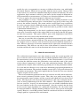
5. DISCUSSION . . . . . . . . . . . . . . . . . . . . . . . . . . . . . . . . . . . . . . . . . . . . . . . . . . . . .
5.1. Evaluation of the system . . . . . . . . . . . . . . . . . . . . . . . . . . . . . . . . . . . . . . . .
5.2. Improvements proposed to the system . . . . . . . . . . . . . . . . . . . . . . . . . . . .
5.3. About the measurements . . . . . . . . . . . . . . . . . . . . . . . . . . . . . . . . . . . . . . . .
50
50
51
52
6. SUMMARY . . . . . . . . . . . . . . . . . . . . . . . . . . . . . . . . . . . . . . . . . . . . . . . . . . . . . . . 54
7. REFERENCES . . . . . . . . . . . . . . . . . . . . . . . . . . . . . . . . . . . . . . . . . . . . . . . . . . . . 55
8. APPENDICES . . . . . . . . . . . . . . . . . . . . . . . . . . . . . . . . . . . . . . . . . . . . . . . . . . . . . 58
FOREWORD
This thesis has been carried out as a part of the 5G radio access solutions to 10 GHz
and beyond frequency bands (5G to 10G) project. The project is supported by Broadcom Communications Finland Oy, Elektrobit Wireless Communications Oy, Huawei
Technologies Oy (Finland) Co. Ltd, Nokia Networks Oy and Finnish funding agency
for innovation (Tekes). I would like to take this opportunity to thank all the project
partners for their competence for this work.
I would also like to thank my technical advisor M.Sc (Tech.) Veikko Hovinen for
the great ideas leading to this work. I am graceful for the thesis examiners Lic.Sc
(Tech) Risto Vuohtoiemi and D.Sc (Tech.) Juha-Pekka Mäkelä for reading the thesis
and advising me in writing. I would also like take this opportunity to thank Professor
Matti Latva-aho for the trust to my abilities to work here, D.Sc (Tech.) Marko Sonkki
for helping me in the beginning of my work, Anssi Rimpiläinen for implementing the
most of the mechanics and M.Sc (Tech.) Claudio Ferreira Dias for the great technical
discussion during the work. Furthermore, I would like to thank all the Centre for
Wireless Communications staff for feeling me welcome to work here.
I would also like to take this opportunity to thank my family and friends for all the
support I have enjoyed during my University studies. Especially, I would like to thank
my brothers Valtteri and Oskari for the everyday discussion, help and support during
the studies as well as during the time spend with this thesis. The special thanks goes
to my girlfriend Jenny for the sincere support and understanding towards my passion
for science for all the years we have been together.
Oulu, Finland October 24, 2014
Nuutti Tervo
LIST OF ABBREVIATIONS AND SYMBOLS
AC
AoA
AoD
DC
DoA
DoD
GO
GPS
GTD
GUI
IDFT
IF
IFFT
IP
KED
LAN
LNA
LOS
MCode
MIMO
NLOS
PA
PDF
RF
RMS
RT
RX
SCPI
S-parameters
TCP/IP
TX
UTD
VNA
3D
5G
alternating current
angle of arrival
angle of departure
direct current
direction of arrival
direction of departure
geometrical optics
global positioning system
geometrical theory of diffraction
graphical user interface
inverse discrete Fourier transform
intermediate frequency
inverse fast Fourier transform
internet protocol
knife-edge diffraction
local area network
low noise amplifier
line-of-sight
machine code
multiple input multiple output
non-line-of-Sight
power amplifier
probability density function
radio frequency
root mean square
ray tracing
receiver
standard commands for programmable instruments
scattering parameters
transmit control protocol/internet protocol
transmitter
uniform theory of diffraction
vector network analyzer
three dimensional
fifth generation
a1
a2
B
BC
BD
BIF
Bmeas
b1
b2
signal entering to the 2-port input
signal leaving from the 2-port output
bandwidth
coherence bandwidth of the channel
doppler bandwidth
intermediate frequency bandwidth
measurement bandwidth
signal reflecting from the 2-port input
signal reflecting from the 2-port output
C(ν)
c0
D
Das (θd )
D(θ, φ)
d
dm
d0
d1
d2
E(r)
E0 (θ, φ)
e
ecd
er
e0
Fcas
FN
F (ν)
f
fn
f0
G
GR
GT
G(θ, φ)
Gabs (θ, φ)
H
H
H(f )
hF
hij
hlm
h(t)
I0
j
Kr
k
k
kB
L
Lf s
Lke
Lm (d)
Lref
NF
N FVNA
Fresnel cosine integral
light speed in vacuum
largest dimension of an antenna
absorbing screen diffraction coefficient
antenna directivity
distance
distance that the wave has propagated in the medium
reference link distance
distance from the TX
distance from the RX
electrical field vector as a function of r
electrical field vector at distance r = 0
Neper number
antenna radiation efficiency
antenna reflection efficiency
total antenna efficiency
total noise figure of cascaded RF-blocks
noise factor
knife-edge diffraction coefficient
frequency
n:th recorded frequency sample
center frequency
gain
RX antenna Gain
TX antenna Gain
antenna gain
absolute antenna gain
height of an obstacle
MIMO channel matrix
channel frequency response
radius of first Fresnel ellipsoid
channel coefficient from TX antenna i to RX antenna j
impulse response between ports l and m
channel impulse response
Bessel function
imaginary unit
Rician K-factor
wave number
complex wave number
Bolzmann constant
path loss
free space path loss
knife-edge diffraction loss
loss in the dielectric medium
path loss at the reference distance
noise figure
noise figure of VNA
Nblocks
NFr
N0
nR
nRx
nRy
nT
nTx
nTy
n1
n2
P
P DP
PN
PR
PS
PT
RA
RL
Rr
R⊥
Rk
r
rf
Slm (fn )
SN R
SN Rin
SN Rout
S(ν)
S11
S21
T
TC
Tcas
Te
T⊥
Tk
T0
t
XA
P LF
X(f )
x(t)
Y (f )
y(t)
ZA
number of RF blocks in the RX chain
number of frequency points
noise power delivered to the output
number of RX antennas
number of RX antennas into x-direction
number of RX antennas into y-direction
number of TX antennas
number of TX antennas into x-direction
number of TX antennas into y-direction
refraction coefficient for the medium 1
refraction coefficient for the medium 2
power
power delay profile
noise power
received power
signal power
transmitted power
antenna resistance
antenna loss resistance
antenna radiation resistance
reflection coefficient for perpendicular polarization
reflection coefficient for parallel polarization
distance from the antenna
far field distance
S-parameters measured between ports l and m
signal-to-noise ratio
signal-to-noise ratio at the input
signal-to-noise ratio at the output
Fresnel sine integral
reflection coefficient of the 2-port input
transmission coefficient of 2-port
physical temperature in Kelvins
channel coherence time
total noise equivalent temperature of cascaded RF-blocks
noise equivalent temperature
transmission coefficient for perpendicular polarization
transmission coefficient for parallel polarization
room temperature in Kelvins
time
antenna reactance
Polarization loss factor
transmitted signal frequency response
transmitted signal in time domain
received signal frequency response
received signal in time domain
antenna impedance
γ
γp
∆d
∆t
δd
δt
tan δ
0r
00r
0
1
2
θ
θd
θi
θr
θt
λ
µ
ν
ξ
ρp
ρpA
ρpW
σ
τ
τ̄
τRMS
φ
Ωr
ω
path loss exponent
propagation constant
maximum detectable path distance
maximum detectable path delay
path distance-resolution
path time-resolution
loss tangent
permittivity
real part of the permittivity
imaginary part of the permittivity
vacuum permittivity
permittivity of the medium 1
permittivity of the medium 2
elevation angle
diffraction angle
incident angle
reflection angle
transmitted angle
wavelength
permeability
fresnel diffraction parameter
auxiliary integral variable
polarization vector
polarization vector of the antenna
polarization vector of the wave
electrical conductivity
delay
mean delay spread
RMS-delay spread
azimuth angle
Rayleigh distribution parameter
angular frequency
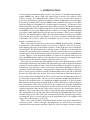
1. INTRODUCTION
In the modern telecommunication systems, the presence of multiple-input multipleoutput (MIMO) has taken a huge role when trying to increase the capacity of the
wireless systems. In a multipath radio channel, one way to increase the capacity is
to increase the number of antennas beyond the antenna configurations used nowadays.
This concept is often called as massive MIMO were transmitter (TX) and receiver (RX)
could be equipped with hundreds or even thousands of antennas. [1] Because of the
limited frequency spectrum, many of the future fifth generation (5G) mobile communication applications will use higher frequencies for the communications approaching to
the millimeter-wave region. High frequencies allows to use larger bandwidth making
it possible to offer higher data rates for the users in the future. Also, because of higher
path loss, the high frequencies allows the telecommunication systems to use smaller
cells and thus decrease the reuse distances. In order to perform reliable link budged
calculations and be able to ensure the availability, the need of new reliable channel
models is undisputed. [2] [3]
There exists only few good ways to measure the MIMO channel reliably. In MIMOmeasurements, radio channel sounders are often used. However, there are few drawbacks limiting the usage of the channel sounders, such as high prize and synchronization problems. The drawback in most existing systems is that they does not take into
account the correlation between antennas, since the measurements are not performed
simultaneously between all antennas, which is often the case in real telecommunication
systems. However, if the measured channel is assumed to be constant with respect to
time, the MIMO channel model can be constructed by measuring each single antenna
channel between the antenna elements separately one by one. [4]
One good way to measure the radio channel is to use vector network analyzer (VNA)
with virtual antenna arrays in both the TX and the RX ends. Only few physical antenna
elements are used and the antenna is moved between different positions to represent a
real antenna array. Robotics can be used to move the antenna making the actual measurement smooth and automatic. Advantage here compared to the channel sounders is
that we do not need to perform external synchronization between the TX and the RX,
because the VNA takes care of that. One serious drawback in VNA-based measurement systems is that the RX and the TX are in the same box meaning that we have to
use long radio frequency (RF) -cables to be able to measure trough long link distances.
However, this problem comes less significant in higher frequencies as the reasonable
link distances are decreasing, meaning smaller cell size. Especially, at indoor propagation environment, VNA based systems can be successfully used. Another drawback in
virtual antenna array based measurement systems is the increased measurement time.
Antenna movement between the VNA sweeps increases the measurement time significantly. The sweep time of the VNA is proportional to the intermediate frequeny
(IF) -bandwidth used. On the other hand, increasing the IF-bandwidth decreases the
dynamic range of the VNA. The trade of between the needed dynamic range and the
measurement speed is needed and the overall performance has to be optimize with
respect the desired property. [5] [4] [6]
There exists many references describing virtual antenna array based channel measurement systems. Various strategies and equipments are used to move the antenna
element between the antenna positions. However, there exits huge variations in mea-
11
surement speed and accuracy between the existing systems. Many of the existing systems uses a rotator or an XY-gantry or both of them. Using the rotator, cylindrical
arrays can be made and the array is also capable to see to the backside beam. Rotator is used for example in [4] which represents capacity measurements using large
antenna arrays. Planar antenna array configurations with a XY-gantry are used in [6]
and [7] describing channel measurements in frequencies 2.4 GHz and around 60 GHz.
In paper [6], optical fibre is used to degrease the cable loss in VNA-based system.
There has been made some research and channel models about the indoor radio
channels on millimeter-wave region. However, the most of the research and channel
models focuses on higher or lower frequencies than 10 GHz. The measurements performed in the higher frequencies are mostly focused to 17 GHz, 28 GHz, 38 GHz and
60 GHz. Especially in 60 GHz, there are large unallocated frequency bands, which
some applications of the future telecommunications systems could use. Many indoor
measurement campaigns and models are made for those frequencies because those
bands are potential frequency regions for future wireless local area networks (LAN).
Paper [8] presents channel measurements made on 10 GHz at indoor environment
and compares them to the statistical channel models. In the paper, the authors presents
measurement results of the received power envelope. Measurement results are fitted to
the Rayleigh, Rician and Nakagami distributions. The paper concludes that the probability that the received envelope power is below some threshold follows the Nakagamidistribution with a good precision. The Rayleigh and Rician distributions were concluded to fit weakly to the 10 GHz statistical indoor channel model. The paper presents
only received envelope power measurement results and channel characteristics such as
multipath delay spread were not calculated based on the result.
Paper [9] presents large scale parameters of wideband multipath channels. The models made by the measurements are based on extensive measurement campaigns in various indoor environment. The measurements were done by using wideband MIMO
channel sounder having 400 MHz bandwidth at 11 GHz. The paper characterizes the
polarization characteristic of path loss, shadowing factor, cross-polarization power ratio, delay spread and coherence bandwidth of the channel. The paper states that the
path loss exponent is between 2 and 3 in non-line-of-sight (NLOS) environment and
between 0.36 and 1.5 in line-of-sight (LOS) environment, respectively. The path gain
in vertically and horizontally polarized transmissions are stated to be almost the same
in most of the measured environments. In some special corridor-rooms the path loss
for horizontally polarized wave is stated to be significantly large. The measurement
campaign presented in the paper [9] is conducted in the university building in 3 different corridor-rooms and 2 different halls and the both LOS and NLOS scenarios are
considered.
The approach to the channel modeling and the measurements presented in the paper
[9] is almost similar compared with the one that we had. However, using VNA with
virtual antenna arrays instead of MIMO channel sounder sets its own limitations for
the measurement system. On the other hand it also gives a number of advantages
compared to channel sounder.
This thesis is organized as follows. In Chapter 2, some background theory related
to the electromagnetic waves and radio channel models are carried out. Chapter 3
introduces the used measurement setup and how it was built. In Chapter 4, some
channel measurement scenarios and initial results are introduced. In Chapter 5 the
12
measurement system is evaluated and some improvements to the system are proposed.
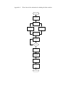
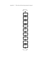
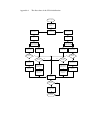
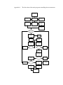
The conclusion is drawn in the Chapter 6. Some flow charts of the measurement control
software and the inputs defined by the user are found from the Appendices at the end
of this thesis.
13
2. RADIO CHANNEL CHARACTERISTICS
The radio wave undergoes many physical phenomena caused by the radio channel
before reaching the RX. These phenomena depends on the wave properties such as
frequency as well as the properties of the propagation environment. In a multipath
channel, the wave propagates trough several different paths between the TX and the
RX causing fading and shadowing to the received signal. In this chapter, we will
present the basic theory of radio wave propagation phenomena and the radio channels,
respectively. [3]
2.1. Electromagnetic propagation
Understanding the behavior of electromagnetic waves is needed in order to understand
the theory behind existing radio channel models. An electromagnetic wave can be described by the Maxwell’s equations (presented in [10]) by using electrical or magnetic
fields. Usually, the electrical field as a function of time or direction of propagation is
used to describe the wave behavior. The nature of the electromagnetic wave observed
in very near to the source is different compared to the nature of the same wave after
it has been traveled over relatively large distance. The radiating field region of an antenna can be divided into radiating near field and far field regions. These regions are
also called as Freshnell and Fraunhoffer regions, respectively. In the radiating near
field, the field attenuation is stronger than in the far field. The distance after the field
is referred to be far field is defined as
2DA2
,
(1)
rf =
λ
where DA is the largest dimension of the antenna measured in perpendicular to the
antenna radiation direction and λ is the wavelength of the wave. [11]
2.1.1. Plane waves and spherical waves
When observing the whole wavefront that the antenna is transmitting, the wavefront is
seen as spherical. Electric field of the spherical wavefront can be written as
e−jkr
,
(2)
r
where r is the radial distance from an the antenna, E0 (θ, φ) is the electrical field vector
at distance r = 0 as a function of direction of propagation (θ, φ), k is the wave number
and j is the unit imaginary number. Wave number k can also be expressed as [12]
2π
.
(3)
k=
λ
In the antenna far field region, the spherical wave can be locally approximated as
a plane wave. This is because every source looks like a dot source when observing it
from far enough. The electric field of the plane wave can be expressed as
E(r) = E0 (θ, φ)
E(r) = E0 (θ, φ)
e−jk·r
,
r
(4)
14
where k is a complex wave vector and r is a position vector defining a point in 3D
(Three Dimensional) space. [12]
2.1.2. Polarization
The polarization of the electromagnetic wave describes the time-varying direction and
relative magnitude of the electric-field vector. In the 3D vector-space, the polarization
describes the function of how the electric field vector varies among the direction of
propagation (or ωt-axis). We can classify different kind of polarizations to be linear,
circular and elliptical. When the electric field is oscillated only in one line, the wave
can be said to be linearly polarized. Linear polarization can always be reduced to two
polarization components; vertical and horizontal. In vertical polarization, the electrical
field is oscillating vertically among the y-axis with respect to the direction of propagation (time-axis). In horizontal polarization, the same happens in the horizontal plane,
i.e the electrical field is oscillating among the x-axis. In circular polarization, the electric field goes around the circular orbit over the time-axis with a constant amplitude.
In elliptical polarization, the electrical field vector goes around the elliptical orbit over
the time-axis and the amplitude is also varying. In case of elliptically polarized wave,
we can define the axial ratio of an ellipse that the electrical field vector is tracing. The
axial ratio is the ratio of the magnitudes of the major axis and minor axis. In case of
circular polarization, the axial ratio is one. [13]
The polarization of an antenna is said to be same as the polarization of the radio
wave the antenna is radiated. Therefore, vertically polarized antenna receives poorly
horizontal polarized waves. Same goes the other way around. However, in the radio
channel, the polarization is not always the same in the TX and the RX. Thus, the
polarization can change while the wave is traveling trough the radio channel due to the
different propagation phenomena presented in next Sections. [13]
The polarization vector ρp represents the polarization of the wave. The polarization
vector is simply the unit vector pointing to the direction of the electric field. [13]
2.2. Propagation in the radio channel
By radio channel we mean the whole radio system including the TX, the RX and
the propagation channel. Depending on the channel geometry and the propagation
materials, the radio wave may travel trough several different paths between the RX and
TX. Thus, the radio wave undergoes several radio propagation phenomena between the
TX and RX, which all affects to the wave behavior in the channel. In this section we
will present the basic radio propagation phenomena, which are valid especially for
indoor propagation environment. [14]
2.2.1. Free space path loss
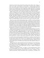
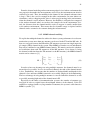
The propagation medium is defined to be free space, when the first Fresnel ellipsoid is
clear from obstacles. In case of some obstacles within the Fresnel zone, the transmitted
15
signal experiences some other propagation phenomena besides free space propagation.
The radius of the first Fresnel ellipsoid is defined as
r
λd1 d2
,
(5)
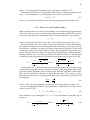
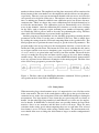
hF =
d1 + d2
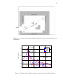
where d1 and d2 are the distances presented in the Figure 1. [14]
Figure 1. The first Fresnel ellipsoid.
If the signal is assumed to be propagated only trough free space, the received power
PR can be represented by Friis equation
λ 2
),
(6)
4πd
where PT is the transmitted power, d is the direct distance between the antennas. GT
and GR are the TX and the RX amplifications, respectively. The path loss Lfs experienced by the wave can be written as [11]
PR = PT GT GR (
Lfs =
4πd 2
1
(
).
GT GR λ
(7)
2.2.2. Plane wave in the medium
The dielectric and the magnetic properties of the medium can be described by parameters µ (permeability) and (permittivity). The permittivity can be complex, when the
imaginary part 00r describes the dielectric losses caused by the medium. Thus permittivity can be represented as
= 0 (0r − j00r ),
(8)
where 0 is the permittivity of the vacuum and 0r is the real part of the relative permittivity. [14]
The dielectric properties of the propagation medium affects to the propagation loss
experienced by the radio wave. The loss caused by the medium can be specified by the
loss tangent of the medium
00r + (ωσ0 )
tan δ =
,
(9)
0r
where σ is the electrical conductivity and ω is the angular frequency [14]. Complex
propagation constant of the medium is represented as
r
σ
√
γp = jω µ 1 − j
= α + jβ,
(10)
ω
16
where α is the propagation coefficient and β is the phase coefficient. [15]
The attenuation of the wave is exponential with respect to complex propagation constant γp . The attenuation Lm (d) of the planar wave can be represented as
Lm (d) = eγp dm ,
(11)
where dm is the distance which the wave has been propagated in the medium. [14]
2.2.3. Plane wave in the media boundary
When a planar radio wave comes to the boundary of two different propagation media,
some part of the wave power is reflected back form the boundary while the rest of the
wave power propagates into the medium. Snell’s law for reflection is represented as
θr = θi ,
(12)
where θr is the angle of reflected wave and θi is the incident angle of the wave. [11]
The polarization of the wave affects to the wave behavior at the media boundary.
The amount of relative power reflecting back form the boundary can be expressed by
the reflection coefficients specified for both perpendicular and parallel electric field
components with respect to the boundary. Hence, the polarization vector of the wave
may be changed due to the reflection, but not the actual polarization. This means that a
linearly polarized wave stays linearly polarized also after the incidence. The reflection
coefficients for the perpendicular and parallel polarizations can be expressed as [16]
q
q
2
− sin2 θi − 12 cos θi
cos θi − 21 − sin2 θi
1
and Rk = q
.
(13)
R⊥ = q
2
2
2
2
2
−
sin
θ
+
cos
θ
−
sin
θ
+
cos
θ
i
i
i
i
1
1
1
As part of the wave is reflected back from the media boundary, the rest of the energy
is propagated trough the boundary inside the medium. The propagation angle of the
wave may change depending on the relation of the dielectric properties of the media.
Thus, the wave undergoes refraction in the media boundary. If we denote θt as the
angle of the refracted wave, the propagation angle can be calculated by the Snell’s law
for refraction
√
1
sin θt
=√ ,
(14)
sin θi
2
where 1 and 2 are the permittivities of first and second propagation medium. [14]
In case of orthogonal incidence, the transmission coefficients of the wave can be
expressed as [16] [14]
T⊥ = 1 + R⊥ and Tk = 1 + Rk .
(15)
If the incidence is not orthogonal, i.e θi 6= 90◦ , the transmission coefficients can be
written as
q
2
cos θi
2
1
2 cos θi
T⊥ = q
and Tk = q
.
(16)
2
2
2
2
2
−
sin
θ
+
cos
θ
−
sin
θ
+
cos
θ
i
i
i
i
1
1
1
17
2.2.4. Plane wave in rough surfaces and diffracting edges
In scattering, the small particles along the propagation path absorbs some energy and
radiates it again to the around space, while acting as small antennas by themselves.
When there are many of these particles along the propagation path, the scattering effect
can be significant and cause fading to the received signal. For example clouds and
bushes are just an examples about obstacles causing scattering. Also rough surfaces,
whose roughness is close to the wavelength, causes scattering. For the scattering, there
exist several models and theorems which are not presented here. Generally speaking,
we can note that the effect of scattering to the radio wave is random and hence must be
modeled statistically. [16]
When some obstacle comes inside the first Fresnels zone, the wave is diffracted from
the edge of the obstacle. If the obstacle is assumed to be wedge-shaped, it can be approximated as a conducting half plane, i.e a knife edge. By the Huygens principle,
every point of a radiating field can be referred to be the dot source of new electromagnetic field. geometrical optics (GO) defines the Snell’s law of diffraction as
n1 sin θi = n2 sin θd ,
(17)
where n1 and n2 are the refractive indices of the media 1 and 2, respectively and θd is
the diffraction angle of the wave. The Snell’s law for diffraction approximate waves
as rays (ray tubes), and it does not take into account the attenuation that the wave
undergoes because of diffraction. [17]
If the knife-edge diffraction (KED) -approximation is used, we can also calculate
theoretical diffraction coefficient. The diffraction parameter ν can be expressed as
ν=
√ H
2 ,
hF
(18)
where H denotes the height of the obstacle with respect to the direct link chord. The
KED-coefficient can be expressed as
1
F (ν) = (1 − (1 − j)(C(ν) − jS(ν))),
2
where C(ν) and S(ν) are Fresnel integrals defined as
Z ν
Z ν
π 2
π
cos( ξ )dξ and S(ν) =
C(ν) =
sin( ξ 2 )dξ,
2
2
0
0
(19)
(20)
where ξ is the auxiliary variable for the integral. [12] Diffraction loss factor is the
absolute value of the diffraction coefficient. To avoid the calculus of complex Fresnel
integrals, approximations can be used to calculate the diffraction coefficient for certain
ν-values. For ν > −0.7, the diffraction loss Lke in dBs can be approximated as [18]
p
Lke = 6.9 + 20 log( (ν − 0.1)2 + 1 + ν − 0.1).
(21)
Instead of modeling the diffraction by wedges by KED, absorbing screen can also be
used to model diffraction. For a plane wave incidence, the absorbing screen approach
18
gives us a geometrical theory of diffraction (GTD) diffraction coefficient with respect
to θd as
√
1 − λ 1
−
.
(22)
Das (θd ) =
2π θd 2π − θd
The wavefront after diffraction is astigmatic because there is some caustic in the edge.
GTD and uniform theory of diffraction (UTD) defines also other similar coefficients
for the diffraction. As well as in the reflection and refraction, the polarization vector
of the wave may be changed due to the diffraction. [16] [12]
2.2.5. Fading and shadowing
Fading is defined as the deviation in radio channel causing attenuation to the transmitted wave. In a rich multipath channel, the transmitted wave propagates trough many
different propagation paths causing deviation to the received signal. All multipaths are
summed in the RX by the superposition principle. Fading can occur in time-, spaceand frequency domain and it can be modeled statistically. Thus, fading is a random
process whose quantities depends on the propagation environment and mobility in the
channel. [3]
In Rician fading, Rice-distribution is used to describe the randomness of the channel.
Rician fading is used, when one of the received multipath components are relatively
strong compared to others. Typical case of Rician fading is the LOS-environment. The
Rician distribution is a function of two parameters, Kr and Ωr . The probability density
function (PDF) of the Rician distribution is defined as
s
2
2(Kr + 1)x
2(Kr + 1)x
2(Kr + 1)x
exp(−Kr −
)I0 (2
),
(23)
f (x) =
Ωr
Ωr
Ωr
where Kr is said to be a Rician K-factor defined as the ratio of the strongest multipath
(typically LOS) compared to other multipaths, I0 is the Bessel function and Ωr is the
total power of all the propagation paths. [19]
Rayleigh fading is typically used in NLOS-environment. In the Rayleigh fading,
the magnitude of the received signal follows Rayleigh distribution described by the
parameter Ωr . The PDF of Rayleigh distribution can be written as [19]
f (x) =
x2
2x
exp(− ).
Ωr
Ωr
(24)
2.3. Radio channel modeling
The radio channel models are usually defined to deterministic and stochastic channel
models. Some of them are defined based on theory while others are based on the measurement data. The stochastic models relay on statistical distribution of the channel,
while deterministic models tries to model the path loss in the channel deterministically
by using for example the geometry of the propagation environment. In geometry based
deterministic channel modeling ray tracing (RT) is often used. By the RT we mean the
19
geometry based radio wave path estimation between the TX and RX. In this section we
present some key parameters and theory related to radio channel modeling.
2.3.1. Frequency and impulse responses
The channel frequency response is used to describe the channel behavior as a function
of frequency. When multiplying transmitted signal spectrum X(f ) by the frequency
response H(f ), we get the received signal spectrum Y (f ). In frequency domain this
can be expressed as [20]
Y (f ) = H(f )X(f ).
(25)
In time domain, the channel is described by the channel impulse response h(t). The
impulse response is the inverse Fourier transform of the frequency response, hence the
received signal y(t) in time domain can be expressed as
y(t) = h(t) ∗ x(t),
(26)
where x(t) is the transmitted signal and (∗) denotes the time domain convolution of
the signals. [20]
In the radio channel modeling, the power of different signal paths is often interesting. Power delay profile (P DP ) of the channel is defined by the impulse response
representing the powers received at each time instant. It can be written as [3]
P DP (τ ) = |h(t)|2 .
(27)
2.3.2. Delay spread, doppler spread and angular spread
There are few parameters to describe the properties of the multipath channel. Delay
spread is a measure of the multipath richness of the propagation channel. It is defined
by the P DP as being the time difference between the earliest and the latest significant
multipath component seen in the received signal P DP . In LOS-channel, the earliest
component is the LOS-propagated component of the signal. Mean delay spread and
root mean square (RMS) -delay spread are parameters describing the deviation of the
received signal path delays. The mean delay spread is defined as [3]
R∞
τ P DP (τ )dτ
,
(28)
τ̄ = R0 ∞
P
DP
(τ
)dτ
0
where τ is the delay at each multipath component. The RMS-delay spread is defined
as [3]
sR
∞
(τ − τ̄ )2 P DP (τ )dτ
0 R
τRMS =
.
(29)
∞
P
DP
(τ
)dτ
0
The coherence bandwidth of the channel can be defined as the Fourier transform of
the delay spread. The coherence bandwidth defines the bandwidth which the channel stays constant with respect to frequency. Roughly, it can be approximated by the
inverse of the mean delay spread [3]
BC ≈
1
.
τ̄
(30)
20
If the TX, the RX or the environment is in motion over time, the transmitted signal
experiences Doppler effect. Thus, in the received spectrum (Doppler spectrum), several frequency components may be seen even if only one was transmitted. The spread
of the frequencies in the RX caused by the Doppler effect is called as Doppler spread.
The width of the Doppler spectrum is called as Doppler bandwidth, BD [3] [17]. Channel coherence time TC is inversely proportional to the Doppler bandwidth and it can be
written as [3]
1
.
(31)
TC ≈
BD
In a multipath channel, the multipath propagated components leaves from the TX
antenna and arrives to RX antenna in some specific angle with respect to some reference direction, which is usually the direct link path between the TX and RX. These
angles are called as angle of departure (AoD) and angle of arrival (AoA), respectively.
In three dimensional (3D) space, AoA and AoD is often defined separately for azimuth
and elevation domains. Thus, the azimuth and elevation angles can be extended into
3D as direction of arrival (DoA) and direction of departure (DoD). The Angular spread
is a parameter to describe the spatial order of the channel. [3]
2.3.3. Deterministic channel models
The deterministic channel models tries to estimate the path loss and phase difference
experienced by the signal as it propagates trough the channel. The deterministic path
loss models, such as the free space path loss model presented in (7), are used to calculate the path loss of the channel. The models include a number of approximations and
all of the radio propagation phenomena are not usually taken into account. This means
that we have to simplify the geometry of the environment in order to estimate the most
significant multipaths from the impulse responses. The models are parameterized to fit
to the propagation environment.
One deterministic channel model, the simplified path loss model, is defined as
L = Lref − 10γ log10 [
d
],
d0
(32)
where L is the path loss, γ is the path loss exponent, Lref is the path loss at the reference
distance d0 and d is the distance in meters. [3]
2.3.4. Indoor channel modeling
The indoor environment has many characteristics making them different from outdoor
environment. At indoor environment, the walls are limiting the radio wave propagation
especially in higher frequencies, because of high wall penetration loss. On the other
hand, the walls gives a possibility to isolate the area better and hence avoid interference coming from outside or other rooms. The reflection, diffraction and free space
propagation are the main propagation phenomena at the indoor environment if the penetration loss of the walls are assumed to be high. Long corridors makes it possible to
transmit signals trough multiple reflections from the source to the destination. [3]
21
From the channel modeling and measurement point of view, indoor environment has
two properties that makes the measurements easier. First, the environment can often be
referred to be static. Thus, the mobility in the channel is low (channel coherence time
is large). This is the case for example in the office environment. In some indoor environments, such as shopping malls, there is often people moving in the environment,
when the channel is static anymore. However, the mobility is still quite low compared
to the outdoor channels where we can have for example cars in the environment. Second, the distances that the channel models needs to support is usually smaller than
at the outdoor environment. This means that less dynamic range is required and the
channel can be assumed to be constant during the measurements.
2.3.5. MIMO channel modeling
To exploit the multipath channel to achieve the better system performance in a telecommunication system, more than one antennas can be used in the TX and the RX ends. In
that case, one pair between the RX and the TX antennas represents one single input single output (SISO) channel in the system. Thus MIMO system has several subchannels
that can be combined to one MIMO-channel matrix. The matrix consists the subchannel coefficients from each TX antenna to all the RX antennas. If we denote hij being
the channel coefficient from the TX antenna i to the RX antenna j, the MIMO-channel
matrix can be written as [3]


h1,1 h1,2 · · · h1,nT
 h2,1 h2,2 · · · h2,n 
T 

H =  ..
(33)
..
..  .
.
.
 .
.
.
. 
hnR ,1 hnR,2 · · · hnR,nT
In order to have an advantage on using multiple antennas, the channels must be as
uncorrelated as possible. In case of correlated channel, the rank of the channel matrix
is low. Furthermore, this means that the number of distinguishable multipaths in the
channel is low and hence MIMO cannot be successfully employed for beamforming.
The best advantage of using multiple antennas is exceeded when the channel is as rich
as possible, meaning high rank of the channel matrix H.
Especially in the future telecommunication systems, the number of antennas are
increased in order to exploit better the multipath richness of the channel. If the TX
and RX are equipped with very large number of antennas, the system is called massive
MIMO -systems. [1]
22
3. RADIO CHANNEL MEASUREMENT SETUP
When measuring the MIMO channel, the measurements with a good accuracy with
respect to the dynamic range of the system may take a significant amount of time. In
massive MIMO systems where both ends contains hundreds of antennas, the increase
of amount of measurement time is multiplicative with respect the number of antennas. Furthermore, increasing the number of antennas increases the amount of recorded
measurement data.
One key design principle of the designed measurement system was to do the system
as versatile as possible so that it could be applied to several channel measurements in
the future. We wanted to parameterize the software so that the system supports various
measurement options chosen by the user.
In this chapter, we introduce the measurement system for measuring the MIMO
radio channel at 10 GHz. VNA based measurement setup with virtual planar antenna
arrays in the RX and the TX ends is presented. The programming of the devices is
introduced, but the actual MATLAB implementations are not included to this thesis.
However, some flow charts of the measurement control software are found from the
Appendix.
3.1. VNA based measurement system
There are only few good ways to measure the radio propagation channel. When measuring a MIMO channel, channel sounders are usually a useful devices to be used.
However, there are few drawbacks limiting the usage of the channel sounders. First
drawback is the prize of the apparatus. The commercial channel sounders are expensive and are not always easily available for high frequencies. Second drawback is the
synchronization of the RX- and TX clocks. Even though the high precision rubidium
clocks were used, there is still some imprecision in timing. The third problem is the
large antenna arrays used for the measurements. For every frequency range measured,
specified antenna array has to be designed individually.
Other good possibility is to use VNA with virtual antenna array. Now, only few
physical antenna elements are used and the antenna is moved between positions to
represent an antenna array. One drawback is that the produced measurement result
does not take into account the correlation between antennas in the one end. On the
other hand, simple measurement setup can be used with the device that can be later
on applied to the various applications. Furthermore, the system can be scaled to other
frequencies simply by changing the VNA parameters and using different antennas. If
the VNA:s own frequency range is not enough, mixers can be used to increase VNA
frequency range. However, using external mixers may increase the system noise as
well.
One drawback in virtual antenna array based systems is the increased measurement
time. Antenna movement between the VNA sweeps increases the measurement time
significantly. Also if narrow IF-bandwidth was used, one sweep would take hundreds
of milliseconds of time. The trade of between the needed dynamic range and the
measurement speed is needed and the overall performance has to be optimized with
respect the desired property. [5]
23
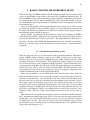
3.1.1. The proposed measurement setup
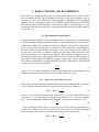
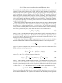
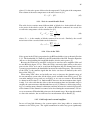
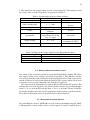
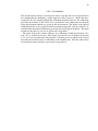
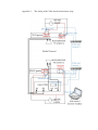
A block diagram of the measurement system is shown in Figure 2. Idea is to use centralized control software, such as MATLAB with instrument control toolbox to control
the devices and store the measurement data. The data flow between the devices is performed via Ethernet bus by using transmit control protocol/internet protocol (TCP/IP)
-communication protocol. The control program should be designed in such a way that
it initializes the measurement, performs the desired VNA sweeps and moves the antennas to another location. The used VNA was Rohde & Schwarz ZNB20 [21]. VNAmeasurement and the antenna moving has to be synchronized such that the antennas
doesn’t move while the VNA is performing the sweep. The S-parameter measurement
data measured by the VNA is transferred to the MATLAB as fast as possible and the
software takes care of the data flow and indexing.
Figure 2. Block diagram of the measurement system.
3.1.2. Scattering parameters
Scattering parameters (S-parameters) are used to describe the effects of an RF-device
or the radio channel to the radio wave. They can be measured by VNA by connecting
the antennas to the VNA ports. S-parameters can be defined theoretically for 2-port
meaning a box with an input and output. Let us denote the incoming wave to the input
port as a1 and wave seen at the output port as a2 . Furthermore, let us denote the wave
24
reflecting back towards the input and output ports as b1 and b2 , respectively. For the
S-parameters, we can write
S11 =
a2
b1
and S21 = .
a1
a1
(34)
Similar coefficients than (34) can be defined for wave coming to the output port. S21
can be referred to be the transmission coefficient of the 2-port and S11 as the reflection
coefficient of the input port. S-parameters can be expanded for n-port as they were
defined for 2-port. [11]
3.1.3. VNA time domain analysis
S-parameters are usually presented in the frequency domain. The transition from frequency domain to time-domain can be done via inverse Fourier transform. There are
two possibilities to get impulse responses out from the VNA. Many analyzers allow
to measure the impulse responses directly in time domain, which are also called as
time domain S-parameters by VNA vendors. However, we decided to measure the
parameters in frequency domain and transform them into time domain via inverse discrete Fourier transform (IDFT). Let us denote Slm (fn ) as the frequency domain Sparameters, where l and m are the port indices and fn is the n:th recorded frequency
sample. By the IDFT, impulse responses hlm can be written as
hlm (tn ) =
1
Npoints
Npoints −1
X
Slm (fk )ei2πkn/Npoints ,
(35)
k=0
where tn is the n:th time instant and Npoints is the number of frequency points [22].
The measured bandwidth in frequency domain determines the time resolution in
time domain. Inverse fast fourier transform (IFFT) algorithm is used to calculate the
IDFT. When using direct IFFT for the frequency domain samples measured by VNA,
we obtain a time resolution of
1
δt =
,
(36)
Bmeas
where Bmeas is the measured bandwidth. In time domain, the number of points, Npoints ,
is the same as in frequency domain, if zero padding is not performed while executing
IFFT. Zero padding increases the resolution, but not accuracy because of interpolation
and thus it should not be used in case of measured data. Thus, the length of the impulse
response is written as [23]
∆t = (Npoints − 1)δt.
(37)
The distance resolution of the recorded impulse responses can roughly be calculated
as
δd = δtc0 ,
(38)
where c0 denotes the light speed in the free space. The length of the impulse response
in distance domain, i.e the maximum detectable path can be written as
∆d = ∆tc0 = (Npoints − 1)δd.
(39)
25
3.2. Dynamic range of the measurement system
For each measurement, one should ensure that the dynamic range offered by the measurement system is reasonable for performing successful radio channel measurements.
The dynamic range of the channel measurement system is defined as the difference
between the highest and the lowest attenuations that the system is able to measure.
When observing the lower limit, one should avoid the RF-components to drive into
compression. On the other hand, the attenuation caused by the channel should be less
than the maximum attenuation supported by the system in order to be able to distinct
the actual signal from the noise. [5]
3.2.1. Noise in the measurement system
In reality, there is always some noise caused by the device in the radio system. There
are different kind of noise sources in RF-electronics. The most significant one in radio
frequencies is the thermal noise caused by the resistive components. The thermal noise
is white, meaning that it remains constant over frequency. The power of the thermal
noise depends on the bandwidth B and the physical temperature T and can be written
as
PN = kB T B,
(40)
where kB is the Bolzmanns constant. It is usually assumed that T = T0 which is the
same as the nominal room temperature. [11]
Signal-to-noise ratio (SN R) is used to describe the signal versus noise quantity. It
is defined as
PS
,
(41)
SN R =
PN
where PS and PN are the signal and noise powers, respectively. [14]
3.2.2. Noise factor, noise figure and noise temperature
For the radio devices, such as RX, we can define parameters to describe how much
noise is appended to the system by the specific device. In an RF-amplifier, both the
signal and the noise are amplified to the output. The noise factor can be defined as
FN =
SN Rin
,
SN Rout
(42)
where SN Rin and SN Rout are the signal-to-noise ratios at the input and output. The
noise figure is the noise factor expressed in decibels and it can be written as [11]
N F = 10 log10 FN .
(43)
Noise equivalent temperature Te describes the thermal noise existed in a radio block.
For a radio component, it can be defied as
Te =
N0
,
GkB
(44)
26
where N0 is the noise power delivered to the output and G is the gain of the component.
The relation of the noise temperature to the noise factor is [11]
Te = (F − 1)T0 .
(45)
3.2.3. Noise in cascaded radio blocks
The radio device consists many different kind of blocks in a chain which all affects
to the noise of the whole system. In a chain of RF-blocks connected in cascade, the
overall noise temperature can be calculated as [11]
Tcas = Te1 +
NX
blocks
i=2
Tei
Qi−1
j=1
Gj
,
(46)
where Nblocks is the number of blocks connected in cascade. Similarly, the overall
noise factor of the cascaded chain can be defined as
NX
blocks
Fi − 1
Fcas = F1 +
(47)
Qi−1 .
j=1 Gj
i=2
3.2.4. Noise in the VNA
Noise power in the VNA is proportional to its RX bandwidth as it was shown in Section
3.2.1. The bandwidth B is limited by the IF-bandwidth of the RX. From the Equation
(40) we see that doubling the bandwidth doubles also the noise power. [5]
Because the VNA has its own RX, it also has its own low noise amplifier LNA and
its own RX noise figure N FVNA . Thus, the VNA:s own noise figure affects to the noise
power in the VNA. As it can be seen from the Equation (40), the thermal noise in the
system is proportional to the bandwidth, but not to the actual frequency. The sensitivity
of the VNA, i.e the smallest signal that the device can detect is limited by the noise
floor of the VNA. [5]
When using VNA, there are basically two ways to increase the dynamic range of
the measurement system after all the input power available from VNA is used. We
can make multiple sweeps and use averaging, or we can use narrower IF-bandwidth
as shown in the Section 3.2.4. Both methods increases the measurement time significantly. It is often said that the effect to the measurement time and dynamic range is
roughly the same no matter which method was used. [5] However, when using averaging, we consider many channel realizations and thus measure the statistical properties
of the channel. If the channel is assumed to be fixed during the measurements, it is better to use narrower IF-bandwidth to increase the dynamic range. By using this method,
we loose the statistics, but we will have less measurement data to handle. [5]
3.2.5. Link budget and external amplifiers
In case of long link distances, the system requires also long cables to connect the
antennas to the VNA ports. The signal attenuation in cables may grow significantly
27
large and hence reduce the dynamic range of the measurement system. As mentioned
before, increasing the dynamic range of the system by averaging several sweeps or
using narrower IF-bandwidth in the VNA increases also the measurement time. Thus,
using external amplifiers may be necessary to compensate the cable loss and keep the
received signal above the RX sensitivity. [5]
Using external amplifiers causes two problems. As mentioned in the Section 3.2.3,
the additional components in the RX chain increases the noise of the measurement
system. Especially using external LNA in the RX front end increases the RX noise by
its noise figure N FLNA . The overall noise factor (noise figure) can be calculated by
using Equation (47). Also the received signal should always be above the LNA:s own
noise, i.e the sensitivity of the LNA should be adequate for the smallest received signal
level. If the external LNA is used, it has to have better noise figure than the VNA:s
own RX in order to increase the sensitivity of the whole system. Thus, the sensitivity
is not improved directly by the amplification of the LNA. If the LNA is placed directly
after the RX antenna to compensate the long RF-cable, it is useful.
The second problem is how to include the amplifiers into the measurement calibrations in such a way that they will not damage the devices during the calibrations. The
calibration problem can, however, be overcame by adding the amplifiers to the RFchain after the calibrations and canceling them out from the measurements afterwards.
If VNA would support the external amplifier selection by adding it to the rear panel
of the VNA, we could also use that option to compensate the amplifier off from the
results. However, our VNA did not support this option. When using amplifiers, we
also need to ensure that the received power does not reach the level that drives the RX
into compression. Using external amplifiers does not necessarily increase the system
dynamic range, but shifts it down in the power region.
The measurement system should be able to be modified in such a way that the dynamic range must be able to be scalded if needed in order to achieve good speed with
respect of accuracy. The external amplifiers were added to the measurement chain
only if the VNA:s own sensitivity was not enough. This is the case when the long
RF-cables are used causing external attenuation to the signal, hence, decreasing the
dynamic range left for the channel measurements. External LNA could be placed right
after the RX antenna to increase the RX sensitivity. Power amplifier could be placed
right before the TX antenna to increase the transmit power. If the measurement environment requires to use long cables (long links are wanted to be measured) the best
option is to use long cables in both ends. However, this would require that the VNA
should most probably be placed between the antennas inside the measurement environment affecting to the radio channel that is to be measured. Furthermore, the usage of
the TX-amplifier is limited by the maximum power that is allowed to be used according to the radio permission. Also, the power performance of the VNA must be taken
into account such that the overall transmit power does not violate the radio permission.
The idea is to first maximize the transmitted power and then minimize the RX noise.
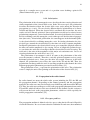
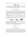
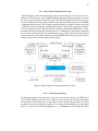
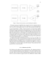
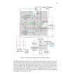
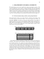
The RF-block chart of the measurement system including the external amplifiers is
presented in Figure 3.
28
Figure 3. Proposed measurement system including the amplifiers.
We propose two types of amplifiers that can mostly be used to compensate the loss
caused by long RF-cables. When using all four RF-ports (for two orthogonal polarizations), two pieces of both amplifier types are needed. The attenuation of the RF-cables
used was approximately 0.9 dB/m. As discussed before, an external power amplifier
should be used in such a way that the radio permission is not violated. The proposed
TX amplifier is HMC-C026 manufactured by Hittite Microwave Corporation. The amplifier gives approximately 29 dB gain at 10 GHz with 1dB-compression point of 25.5
dBm. In order to be able to use the amplifier, one should ensure that the power at the
output of the amplifier does not exceed the compression point. For example, if 15 meter long RF-cable is used in the TX-end, and VNA gives 8 dBm out from the ports, the
total transmitted power would be 23.5 dBm plus the antenna gain. The specifications
of the proposed TX amplifier are presented in [24].
As discussed before, the external LNA can even increase the noise in the RX end, if
short cables are used. Thus, it is not beneficial to use LNA, if the VNA is placed near to
the RX end. However, if long RF-cables are used in RX end, we propose to use LNC0812 LNA manufactured by Miteq. It gives us maximum noise figure of 1.8 dB at 10
GHz with gain of 25 dB at minimum. The overall effect for the RX can be calculated
by Equations (47) if the noise figure of the VNA is known. The specifications of the
proposed LNA are found from [25].
3.2.6. Calibration of the VNA
The VNA has to be calibrated before the measurements. The calibrations should include all of the RF-components used in the RF-chain. If the external amplifiers where
used, they should be included into the calibrations or canceled out from the results
afterwards. There are many possible calibration methods supported by the used VNA.
However, only few of them are supported by the used calibration kit, which was R&S
29
ZV-Z5x [26]. VNA usually measures all of the S-parameters even though only few
of them are selected to be saved into defined traces. The ones not saved into traces,
are dummy measurements, which only increases the measurement time. This means
that we can speed up the measurement by calibrating the VNA only for the parameters
which are supposed to be measured.
Each VNA vendor has their own calibration algorithms. For the radio channel measurements, the best calibration method offered by the used device is one way trough
calibration. However, this option was not supported by the used calibration kit and
thus was not able to be used. Unknown trough open short match (UOSM) calibration
were used instead. [27]
3.3. Virtual antenna array
When measuring the radio channel with the VNA, the number of VNA ports is limiting
the number of simultaneous antennas that could be used. To get still a MIMO channel,
we move the antennas between the sweeps to get a virtual antenna array. The amount
of movement between the measurement points depends on the antenna spacing of the
used antenna array. Because of the channel correlation, usually antenna spacing of half
of the wavelength is used. [13]
There are several ways to perform the antenna movement between the measurement point. Especially in high frequencies such as 10 GHz, the misplacement of the
antennas may cause significant inaccuracy to the measurements. When measuring
large antenna configurations, the best way is to move antennas automatically by using
robotics. Programmable devices such as robotic arms, or stepper motors can be used
for the movement.
We built two XY-gantries to move the TX and the RX antennas to the vertical and
the horizontal directions by using programmable stepper motors. The motors where
chosen such that they could be controlled trough MATLAB along with the VNA.
3.3.1. Antenna characteristics
To be able to distinguish the effect of the propagation channel itself from the measured
data, the effect of the antennas should be compensated off from the data. Since in
reality, antennas are not ideal components, all of the power fed into the antenna is not
necessarily radiated into the space. The impedance of an antenna is matched into the
impedance of the signal source. Thus, the antenna impedance is wanted to be as close
as possible to 50 Ω over the wanted frequency bandwidth in order to radiate well. The
matching of the antenna can be specified by the reflection coefficient S11 . [13]
Reflection efficiency of the antenna takes into account the mismatch between the
transmission line and the antenna. The reflection efficiency can be defined as [13]
er = (1 − |S11 |2 ).
(48)
30
Radiation efficiency of the antenna takes into account the conduction and dielectric
losses of the antenna. The radiation efficiency can be defined as
Rr
,
(49)
RL + Rr
where RL and Rr are the loss and radiation resistances, respectively. [13] The total antenna efficiency takes into account the losses at the input terminals within the structure
of the antenna. Thus, the total antenna efficiency can be written as [13]
ecd =
e0 = er ecd .
(50)
Directivity of the antenna, D(θ, φ), is defined as the ratio of the radiation intensity
in a given direction from the antenna to the radiation intensity averaged over all directions. Gain of the antenna is closely related to the directivity. It is a measure that takes
into account the efficiency of the antenna as well as its directional capabilities. Thus,
the gain can be written as [13]
G(θ, φ) = ecd D(θ, φ).
(51)
By taking into account also the impedance mismatch of the antenna, the absolute gain
of the antenna can be defined as [13]
Gabs (θ, φ) = er ecd D(θ, φ).
(52)
The impedance of the antenna is complex and can be written as [13]
ZA = RA + jXA = RL + Rr + jXA ,
(53)
where ZA is the antenna impedance, RA is the antenna resistance and XA is the antenna
reactance. [13]
The −10 dB bandwidth of the antenna is defined as the frequency range where S11
is less than −10 dB. Polarization of the antenna in a given direction is defined as the
polarization of the wave transmitted (radiated) by the antenna. The polarization of the
radio wave was defined in Section 2.1.2. The polarization loss factor (P LF ) describes
the polarization mismatch between the antenna and the wave. It can be written as
P LF = ρpA · ρpw ,
(54)
where ρpA and ρpW are the polarization vectors of the antenna and the wave, respectively. [13]
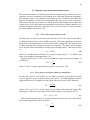
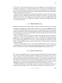
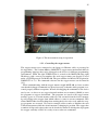
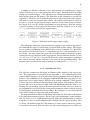
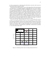
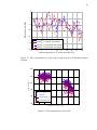
3.3.2. Dual polarized patch antenna
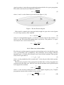
The antennas used for the measurement setup at the TX and the RX were directional
dual polarized patch antennas. The antennas have good impedance matching (< −13
dB) and isolation (> 24 dB) between the feeding ports over the measured 500 MHz
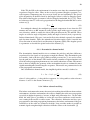
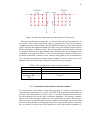
bandwidth. The antenna layout is presented in Figure 4a. The simulated radiation
patterns (XZ-cut) of the antenna polarizations in terms of total gain at 10.1 GHz are
presented in Figure 4b. VNA ports 1 and 3 were connected to the TX antenna, and
ports 2 and 4 to the RX antenna, respectively. The antennas were rotated in such a way
that the orthogonal polarization planes were tilted at ±45◦ angle with respect to the
vertical. The simulated antenna properties are presented in Table 1.
31
(a)
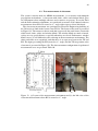
(b)
Figure 4. (a) An overview of the RX/TX antennas and (b) simulated antenna gains of
the two orthogonal polarizations at 10.1 GHz (XZ-cut).
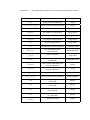
Table 1. Specifications of the antennas used in the measurements
center frequency
10.1 GHz
−10 dB bandwidth
720 MHz
gain
> 4 dBi (boresight)
maximum total gain
5.8 dBi
port isolation
> 24 dB
cross polarization discrimination
> 18 dB
3.3.3. XY-gantry
Stepper motors are used in various applications to control the motion. The precision
of the motors is proportional to the step resolution of the motors. The smaller steps the
stepper can be rotated, the less is the minimum distance that can be moved. To convert
the stepper motor rotation into the linear movement, the linear stage can be used. High
precision linear stages are commercially available to meet the standards of the stepper
motors.
When choosing the stepper motors, programmability and controlling interface were
the most important properties. Other properties, such as step resolution and torque
power were also parameters to be considered. The chosen stepper motor was Lexium
MDrive LMDCE572 with Ethernet interface manufactured by Schneider. The chosen
linear stage was HIWIN KK6005P-600A1-F4. To be able to move both RX and TX
antennas to the horizontal and the vertical directions, 4 stepper motors and linear stages
were needed. The specifications of the motor and the linear stage are represented in
Tables 2 and 3. The hardware manual for the stepper motor is found from [28] and the
programming reference is found from [29]. The manual for the used linear stages is
found from [30].
The function of the limit switches is to limit the motion range of the motors such
that it knows when linear stage is at the maximum or the minimum positions. The
limit switches prevents the motors to push the carriage towards the boundary of the
stage and hence prevents the motors to miss steps as well as broke themselves. The
32
Table 2. Specifications of the selected stepper motors
model
Schneider LMDCE572 NEMA 23
microstep resolution
51200 microsteps/rev
general purpose interface and Ethernet interface
programmable interfaces
(TCP/IP, Ethernet IP, ModbusTCP)
memory
RAM
programming language
MCode
maximum voltage
48 VDC
maximum holding torque
0.86 Nm
maximum required
3.5 A
power supply current
Table 3. Specifications of the selected linear stages
model
KK6005P-600A1-F4
nominal width
60 mm
ballscrew lead
5 mm
rail length
600 mm
resolution
5 mm/rev
maximum speed
340 mm/s
repeatability
±0.003 mm
accuracy
0.020 mm
running parallelism
0.010 mm
starting torque
15 N-cm
limit switches can also be used to define the origin for the steppers when the stepper is
switched on.
Two kinds of limit switches were used in the system. Hard mechanical limiters were
placed to the boundaries of the linear stages to prevent the motor to force the carriage
towards the stage end. These switches were used in both positive and negative ends
of the stages. The switches were connected to the circuit in such a way that the main
current was switched off in case of hard stop.
Inductive proximity sensors were used as soft limit switches. These sensors were
wired to the general purpose programmable interface of the steppers in such a way
that they change register values of the stepper in case of carriage coming close to the
switch (inductive connection). The changed register values can be used in the program
to define interrupt routines that the motor stops the movement in case of reaching the
limit, but stays programmable, which was not possible in case of the hard stop. This
allows the software to use these registers as inputs in programming.
The proximity sensors were also used to define the origo position for the stepper motors. Furthermore, they are also used to define the maximum distance that the carriage
can be moved in stage. The specifications of the used limit switches are presented in
Table 4. The wirings of the stepper motors and limit switches are presented in Figure
33
5. The manual for the used proximity sensors is found from [31]. The settings used in
the voltage sources of the XY-gantries are presented in Table 5.
Table 4. Specifications of the used limit switches
model
GX-F12A-P
VT16061C
switch type
inductive
mechanical
mechanical connection
stable sensing range
0 − 3.3 mm
needed
output operation
normally open
normally open
PNP open-collector
output
passive
transistor
along sensing axis,
perpendicular to sensing
repeatability
not needed
axis: 0.04 mm
can be chosen up to
supply voltage
12 − 24 V
maximum AC 250 V
maximum source current
100 mA
16 A
Table 5. Settings of the voltage supplies of the build antenna spacer
main voltage
30 VDC
main current limit
2A
limit switch voltage
12 V
limit switch current limit
150 mA
3.4. Wiring of the measurement system
The wiring of the overall measurement system including Ethernet routing, RF-cables
and stepper voltage source wiring is presented in Appendix 1. Two Ethernet switches
were used to route the connections between the laptop and devices. Each stepper motor
and the VNA has its own specified Internet Protocol (IP) -address, which can be used
to route the device specific commands into each device separately.
The stands made of aluminium were built for RX and TX antenna XY-gantries. The
antenna mast was made of plastic, and with the stands it allows to use antenna heights
from 1.05 to 2.0 m in the RX end and from 1.50 to 2.80 m in the TX end. Naturally,
the antenna heights can be increased by placing the stands on some external structures.
The whole measurement system in operation is presented in Figure 6.
3.5. Measurement control software
For controlling the devices, MATLAB was used as the programming language. MATLAB instrument control toolbox offers several options to control external devices.
34
Figure 5. Wiring of the stepper motors and limit switches.
TCP/IP-communication protocol over the Ethernet bus is the best option for our purposes, because it is easy to use and is supported by all of the devices used for the measurement system. The communication protocol takes care of the data flow between the
devices and MATLAB. The Instrument control toolbox can be used to debug device
specific languages such as machine code (MCode) and standard commands for programmable instruments (SCPI) to the devices. MATLAB can also be used as a post
processing tool for the measurement results and is therefore an versatile programming
environment for our purposes. [32]
35
Figure 6. The measurement setup in operation.
3.5.1. Controlling the stepper motors
The stepper motors were connected to the laptop via Ethernet cable as presented in
the Appendix 1. The Lexium MDrive LMDCE572 stepper motor understands MCode
programming language that can be debugged to the device via different programming
environment. When the right TCP/IP-object is created to the MATLAB using right
IP-address with a correct port number, the used stepper motor can directly be used
under a TCP/IP-protocol via MATLAB. The port number for MCode/TCP option for
LMDCE572 is 503. The command reference for the stepper motors can be found in
[33].
When communicating with the stepper motors trough MATLAB, we have to make
sure that the debugged commands are queued correctly so that the whole program is executed properly without exceptions. Instead of debugging the commands to the device
one by one, we chose to use stepper internal random access memory (RAM) to store
the programs to steppers beforehand. The programs are stored to the stepper motor
memory spaces to a certain memory addresses and executed from the device memory
by only telling to the stepper from which address is starts to execute commands. This
allows MATLAB to do other things than waiting the device to be ready while the stepper programs are executed. We can for example collect results or initialize the next
VNA measurements while the virtual antenna is changing its position. The stepper has
a number of flags and registers that can be checked to know in which point of program
the stepper currently is and if it is ready or not to take new commands.
36
A number of different subroutines were implemented for controlling the stepper
motors. The first on is to set the origin of the linear stages. The flow chart of the origin
setting is presented in Figure 7. The subroutine uses another subroutine for finding the
limit switches from the XY-gantries. The flow chart of this subroutine is presented in
Appendix 2. The basic idea is to find the move the carriage towards the stage negative
end until it reaches the negative limit switch. The negative limit witch is routed to
the pin 3 (I2 ) of the stepper general purpose interface. As the limit switch is reached,
the voltage in I2 rises up, which is programmed to stop the motor. Then the carriage
is moved a number of steps (offset) to the positive direction, which is set as an origo
(P = 0). Same is done for all of the stepper motors.
Figure 7. Flow chart of the stepper origin setting.
The subroutine writing the stepper movement programs is presented in Appendix 3.
We command the stepper to start writing a program from specific address. The stepper
has its specific programming mode which can be used by command P G. Before the
movement we set the initial speed (Vi ), maximum speed (Vm ) and acceleration (A) to
be suitable. Too large values for speed and acceleration would overload the stepper,
causing missed steps and heats up the stepper motor. The load and run currents (Hc and
Rc) are set to 50% and 100%, respectively. Then the relative movement is performed
into wanted direction and the program is saved into the device RAM memory. The
program can be executed from stepper memory by command EX < address >.
3.5.2. Controlling the VNA
The VNA was connected to the laptop via Ethernet cable similarly to the stepper motors. The connections are presented in the Appendix 1. For controlling the VNA,
standard SPCI-language was used with some external commands offered by Rohde &
Schwarz. The commands can be debugged trough MATLAB in the same way as it was
done in the case of stepper motors. However, here waiting commands (∗ WAI) after the
VNA sweep was used instead of writing the program into the VNA memory. This was
because there were no need to do other tasks with MATLAB while the VNA is performing the measurement. Most of the initial parameters for the VNA was chosen to
be programmed to the VNA by the developed measurement control software, instead
of entering them by hand before the recordings. By doing this we can ensure that all
of the VNA settings are correct for each measurement.
We implemented three different controlling subroutines for VNA that can be utilized
in the main measurement program. The first one is the initialization. In the initialization, the VNA is set to a right measuring mode with right initial parameters. Before
using this, we have to make calibration files available into the device memory. First
we delete all channels from the VNA memory to ensure that no uncorrect parameters would be measured. Then we choose the data transferring mode to be 32-bit real
37
number in binary format. The amplitude and the phase measured will be transferred in
binary format so that even numbers are the amplitudes and the odd ones are the phases,
respectively. Then we create two measurement channels with two traces and select the
sweep mode to be single for all the traces. The analyzer can only sweep one channel at
time, so making two channels with their own calibration pools can decrease the measurement time. Third, we choose the correct calibration pools for both channels to be
used for the measurements. The calibrations pools are automatically set to all of the
traces in the channels. After the calibration pool selection, we set the correct settings
for the VNA, such as frequency region, transmit power, number of frequency points
etc. Finally the VNA is put to a mode to be ready for performing the sweep. The flow
chart of the VNA initialization is presented in the Appendix 4.
Another program we implemented was the checking program for ensuring that the
parameters for the VNA set are the same as defined by the user. This is simply done
by reading the settings from the VNA and comparing them to the specified ones. The
third program was to perform the actual sweeps to get the desired S-parameters. The
program makes two sweeps and saves the measurement data into a vector in the raw
format the VNA provides them. The format for VNA data is such that the odd entries
are real parts and the even ones are imaginary parts, respectively. Both traces (S21 and
S41 or S23 and S43 ) are given in the same vector by one after another. The mode for the
sweep is to make the sweep first and then wait the sweep to be ready before making
another sweep. The saved trace vector is read into MATLAB in binary format and the
traces are separated to two different cell matrices in the main program. The flow chart
of the VNA sweep program is presented in Figure 8.
Figure 8. The flow chart of the MATLAB subroutine commands VNA to perform a
sweep and transfer it from VNA to MATLAB-vector.
3.5.3. Data format
When measuring large virtual antenna arrays, it is unpractical to save all of the results
in the same matrix. The size of the result matrices affect also to the speed of the measurement in case of the data saving from VNA to the MATLAB workspace during the
measurement. Too large matrices slows down the post processing and are clumsy to
handle. On the other hand, large number of small matrices or vectors are also unpractical to handle. In MATLAB, we basically have two possible formats for large block
matrices: One is to use structures and the other is to use cell arrays. There are some
variations in the saving speeds when comparing these two to each other. The selected
data format is to use cell arrays with varying variable names. The measurement software should allow user to change the data format to larger or smaller configuration if
necessary.
38
The selected data format is presented in Figure 9. During the measurements we create cell arrays for each combination of [nRx , nTy , nTx ] with dynamic variable names.
Here nRx and nRy are the number of RX antennas to x and y directions, respectively.
nTx and nTy are the same characteristics for the TX antenna array. The dimension of
these cell matrices are [Npoints , nRy , 2]. Each element of the cell array is 32-bit long
complex number representing one recorded S-parameter value. When we take into
account also the cross polarization products, the result is two group of matrices with
variable name describing the antenna element indices in the TX and the RX ends.
For example cell matrix copol_1_2_3 is the data block measured in antenna positions
Rx = 1, T y = 2, T x = 3 contains Npoints · nRy · 2 complex elements, i.e recorded
S21 and S43 data in measured frequency points at each antenna positions in RX y-axis.
Similarly xpol_1_2_3 is the same result, but the measured parameters are cross polarizations S23 and S41 . The initialization of the result matrices performed in MATLAB
by specific subroutine.
Figure 9. Data format of the saved measurement results.
3.5.4. Error control
For the input-output (IO) error handling, MATLAB is not the best programming environment to do error controlling. The only error handling and interrupt control tool
in MATLAB is the try-catch function. In the current measurement control software
version, we have included only the most necessary error handling.
In order to prevent the MATLAB to jam during the program execution, the whole
measurement control program is set under one big try-catch structure. In case of error,
the actual error message is printed to the display and saved to a log-file. In case of
interrupt or error, the program execution is stopped without exceptions. Basically the
program is terminated in case of any internal or external error. This includes for example that the devices are not connected properly or the device is for example switched
off during the measurement. The recordings made before the error is saved into a
temporary file, from where they can be reloaded again afterwards.
39
3.5.5. User interface
The measurement software is developed in such a way that the user can parameterize
the configuration by modifying a single input file called ’inputs.m’. Before the measurements, the user should perform the calibration manually and save the calibration
pool into the memory of the VNA. User can make his own calibrations for the both
of the measurement channels to speed up the measurement. The name of the applied
calibration file has to be specified in the measurement input file, and the software sets
automatically the defined calibration pools into the measurement channels. The input
parameters that the user can set are given in the Appendix 5.
The main script of the control software uses subroutines defined in Sections 3.5.1
and 3.5.2 to control the devices. The inputs given by the user as defined in Section
3.5.5, are used to parameterize the program. A waiting period is added in the vertical
direction movement because of vibrations of the antenna mast. The flow chart of the
measurement control software is presented in Appendix 6.
40
4. MEASUREMENT SCENARIOS AND RESULTS
The measurement system can be applied for various measurement scenarios. The
recorded S-parameters can be used to calculate information about the propagation
paths, dominating propagation phenomena, channel correlation and many others. The
recorded data can also be used to estimate the DoA and DoD. The used DoA algorithms to analyze the verification measurements are presented in [34]. In this chapter
we represent some examples about the measurement scenarios which for the system
can be used. The measurements were performed in the Oulu University campus area.
4.1. Used measurement settings and the system speed performance
Same measurement settings were used for all of the verification measurements. The
used VNA settings are presented in Table 6. The center frequency, 10.1 GHz, and
bandwidth, 500 MHz, were chosen to satisfy the radio permission. The number of
frequency points used was 201, the IF-bandwidth 10 kHz and the transmit power 8
dBm, which was the maximum power available from the used VNA. According to the
Section 3.1.3, the used VNA settings gives us time domain impulse responses whose
characteristics are presented in Table 7.
Table 6. VNA settings in the verification measurements
f0
Bmeas
BIF
PT
Npoints
10.1 GHz 500 MHz 10 kHz 8 dBm
201
Table 7. Properties of the calculated impulse responses
number of samples
201
delay resolution
2 ns
unaliased length (time)
400 ns
path resolution
60 cm
maximum detectable path length 120 m
In the final measurement system, there are many sources of inaccuracy that must be
considered. The accuracy of the XY-gantry is limited by the used moving equipment
and self build mechanics. For example, the antenna shaking after each movement affects to the accuracy of the antenna location during the measurement. In the systems,
we had to wait some amount of time for the antenna mast to settle. This waiting time
decreased the speed of the measurements. The shaking were observed to be more
significant when moving the antenna in the horizontal direction compared to the vertical direction. This is why the antenna movement pattern where chosen such that the
horizontal movement is minimized. The antenna movement patterns are presented in
Figure 10.
41
Figure 10. The movement patterns of the antennas in XY-gantries.
Along the verification measurements, we measured also the speed performance of
the system. The actual measurement speed is proportional to the selected antenna
configuration and the VNA settings. For the total measurement speed per measurement
point is included the antenna movement, the VNA-sweep and the data transfer from the
VNA to the laptop via Ethernet cable. The measured time per measurement point and
an example about the total measurement times including time for the stepper motor
calibration are presented in Table 8. The used measurement settings for VNA were
presented in the Table 6. Because of the external waiting time of one second added to
the x-direction movement to wait the antenna shaking to settle, we have one second
higher measurement time in the x-direction compared to the y-direction.
Table 8. The measurement system speed measurements
case
time
one point in x-direction
1.9 s
one point in y-direction
0.9 s
test case with antenna
configuration RX: 3 × 3,
2 min 27 s
TX:3 × 3
4.2. Verification measurements in anechoic chamber
To verify that the measurement system works properly, we decided to perform few
verification measurements in as robust and stable LOS-propagation environment as
possible. This measurement can also be used as a reference measurement for the further measurements and for the angle estimation algorithms. The anechoic chamber
placed in the Oulu University campus area was a good place to do this. The measurement system was assembled to the anechoic chamber and the room was isolated from
the most of the reflecting and diffracting surfaces by using absorber pillows. By doing
this, we wanted to ensure only LOS-component is seen in the measured impulse re-
42
sponse. However, the floor of the chamber contained some metal which caused some
reflection in the measurement environment.
The overview of the anechoic chamber is presented in Figure 11. The TX was set to
the right hand corner and the RX was set to left hand corner near the door. The measurements were performed in direct LOS-cases with different antenna configurations
and LOS with the RX rotated 18.8◦ counterclockwise with respect to the direct path.
The rotation of the RX was done for testing the AoA algorithms. The antenna configurations in each measurement case are presented in Table 9. There where no internal
spurious response caused by the measurement system seen in the impulse responses.
Table 9. Antenna configurations for each measurement case in the anechoic chamber
case
1
2
3
4
RX 3 × 3 20 × 20
1×1
20 × 20
TX 3 × 3
1×1
20 × 20
1×1
note
RX rotated 18.8◦
A sample of the measured impulse response in direct LOS-scenario is presented in
Figure 12. In the figure, we have marked out the LOS- and reflected paths, respectively.
As we can see from the figure, the LOS-path is the first arriving multipath component
and it is also the strongest one. The link distance was 4.92 m which for the free space
loss calculated by (7) is 66.4 dB. Both antennas has a gain of approximately 4 dBi in
boresight, so the overall loss here would be 58.4 dB. The measured path loss with antenna gains for the LOS-path seen in the Figure 12 is 60 dB, which corresponds almost
the calculated result. The slight 1.6 dB difference for the measured and calculated result is caused by the antennas, because they are not identical in reality since they are
build by hand in the workshop of the University of Oulu. In the impulse response, we
also see the reflected path. In the reflection, the both of the orthogonal linear polarizations experiences different reflection coefficient according to Section 2.2.3. Thus, for
the reflected path, the polarization vector changes and we have a stronger signal for the
cross polarizations S41 and S23 than for co-polarization.
43
Figure 11. Overview of the anechoic chamber where the reference measurements were
performed.
−50
LOS-path
S21
S43
S41
S23
−60
Reflection from
the floor
Path loss [dB]
−70
−80
RX 0303
TX 0303
−90
−100
−110
0
20
40
60
80
100
Delay [ns]
Figure 12. Sample of the impulse responses measured in the anechoic chamber.
44
4.3. Test measurements in classroom
The system is mostly made for MIMO measurements, i.e to measure rich multipath
propagation environment. A classroom with chairs, tables and window blinds gives
an environment where multiple reflectors and scatterers are present. To test the DoA
and the DoD estimation algorithms, we considered to measure LOS-channel with one
measurement where RX was rotated to 45◦ angle with respect to direct link chord.
The classroom measurement was performed in Electrical Engineering building of
the University of Oulu in the lecture room TS128. The layout of the room is presented
in Figure 13a. The room was chosen such that it represents the usual lecture room with
white board, chairs, tables and window blinds. The window blinds are made of metal,
so they are very good reflectors, especially when they are closed. Furthermore, window
blinds causes as well diffraction and scattering in the measurement environment. The
chairs and tables were organized such that there is an open area between the TX and
RX. The figure presenting the RX (rotated to 45◦ angle) and the TX in operation at the
classroom is presented in Figure 13b. The chosen antenna configurations in performed
measurement cases are presented Table 10.
(a)
(b)
Figure 13. (a) Layout of the measurement environment and (b) the link view of the
classroom measurement where RX is rotated to 45◦ angle.
45
Table 10. Antenna configurations for each measurement case in the classroom
Case
1
2
3
4
5
6
RX 3 × 3
1×1
20 × 20 20 × 20
3×1
3×1
TX 3 × 3 20 × 20
1×1
1×1
1×1
1×1
note
RX at 45◦ P2 terminated P4 terminated
A sample about the recorded impulse responses are presented in the Figure 14. In
these measurements, we had a bug in the measurement control software. The software
did set the correct calibration pool only to channel 2, i.e. only when the VNA port
3 is the TX port. This is seen in the calculated impulse response as a delay offset
as well as wrong signal levels. Thus, we cannot use the recorded S21 and S23 to any
further analysis since the results are corrupted. However, the other polarization can
still be used. The calculated impulse responses shows that in the classroom, there is
many multipaths between the TX and the RX. There is periodical peaks in the impulse
response caused by the multiple reflections. AoA plots will later on show from witch
angle the most significant multipaths are coming from.
−50
S21
S43
S41
S23
−60
Path Loss [dB]
−70
RX 0101
TX 1202
−80
−90
−100
−110
−120
−130
0
100
200
300
400
Delay [ns]
Figure 14. Example of the impulse responses in classroom (S21 and S23 corrupted).
4.4. Wall penetration loss measurements
One application for the measurement setup is to measure the penetration of a concrete
wall by placing the transmitter and RX antennas to different sides of the wall. The
advantage of our system here is that we can easily perform several penetration loss
measurements of the wall with a small spacing between points. The penetration loss
46
of the wall can vary depending on exact location and can contain different materials
such as metallic structures to uphold the concrete. These structures can have a significant effect to the penetration loss. By making several measurements in antenna
positions very near to each other, the fluctuations in the wall structure can be located
and included into the penetration loss measurements. We can also measure the penetration loss in different RX-TX path angles, when the wave incidence to the wall is
not orthogonal. In that case, the part of the transmitted power is reflected back from
the wall causing attenuation to the trough propagated wave. The more we increase the
angle from the orthogonal incidence, the more of the power of the wave is reflected
back from the wall surface. The theory for reflection and refraction was presented in
Section 2.2.2.
The penetration loss of the concrete wall were measured in the two different RXlocations in 3 different antenna configurations. Also LNA was included into the measurement chain for testing the effect of LNA to the dynamic range of the system. The
overview of the measurement setup and environment in seen in the Figure 15a. Also
a reference measurement with a distance of 2.75 meters was performed to cancel the
free space loss off from the results. In the reference measurement, the distance of the
TX and RX antennas was set so that it corresponded the free space distance that the
antennas had in the wall measurement case, thus, the wall thickness was subtracted
from the results.
(a)
(b)
(c)
Figure 15. (a) The wall penetration loss measurement overview and (b) TX and (c) RX
units in operation, respectively.
The analysis of the results can be divided into two parts. At first, we take all the
direct (orthogonal with respect to the wall surface) paths between the RX and the TX
and calculate the wall penetration loss by compensating the free space loss out from
the results channel by channel. For all the used antenna configurations in the both RX
locations, we can do the same.
The penetration loss of the wall is presented in Figure 17. As it can be seen from the
figure, the penetration loss of the wall varies a lot depending on the antenna location.
The variations on the penetration loss seem to be periodical with respect to the antenna
index. The refraction loss of the wall with respect to the refraction angle θt is presented
in Figure 18. Both of the RX locations are collected into same figure. As it was in
47
the direct penetration loss with orthogonal wall incidence, here the results varies also
between the different antenna locations.
The chosen measurement parameters causes following problem. In the measurement
environment, there is multipath propagation causing affecting to the recorded impulse
responses. The measurement bandwidth used (500 MHz) gives only 60 cm resolution
for to distinguish multipaths from each other. In this environment, there is too much
multipath propagation within the resolution bandwidth giving us the a sum of multipaths in each recorded frequency point. When using large bandwidth, the dispersion
of different frequencies might also be a problem in the measurements. However, same
applies for the real communications trough the wall. There might be several reasons,
why the wall penetration loss varies a lot when changing the part of the wall under test.
Thus, plenty of sweeps in each antenna positions would be needed to measure the wall
penetration loss by using this method. Since the variations are so huge, we could also
decrease the antenna spacing and hence get more precise results.
Here the result is that a wall penetration loss can vary a lot depending on the antenna
location even in orthogonal incidence with respect to the wall under test. The variations
in the horizontal direction is observed to be stronger than the variations in the vertical
direction. This may be caused by the structure of the wall as well as the reflections
from the roof and floor. Hence, an office room might not be separated from the other
rooms when considering a communication system where each room has its own BS,
i.e. one cell consists of one room.
2
1.5
Wall under terst
Wall to corridor
TX positions
RX positions
Y-direction [m]
1
0.5
0
−0.5
−1
−1.5
−2
−4
−3
−2
−1
X-direction [m]
0
1
Figure 16. Antenna positions when measuring wall penetration loss.
48
−4
Penetration loss [dB]
−6
−8
−10
−12
sum(S21 ),
sum(S43 ),
sum(S21 ),
sum(S43 ),
−14
−16
0
2
vertical movement
vertical movement
horizontal movement
horizontal movement
4
6
8
10
12
14
16
18
Antenna position in X/Y-direction (RX/TX)
20
Figure 17. The penetration loss of the wall in with respect to X-direction antenna
position.
−50
Path loss [dB]
−55
−60
−65
sum(S21)
−70
sum(S43)
mean(sum(S21))
mean(sum(S43))
−75
−10
−5
0
5
10
15
Refraction angle [deg]
20
Figure 18. The refraction loss of the wall.
25
30
49
4.5. Diffraction around a building corner
The measurement system can be used also for diffraction measurement. When moving
virtual antennas along the x-axis by distance of fractions of the wavelength, we can fast
perform several measurement and see the effect of diffraction for the recorded impulse
response. Also the changes in polarization due to the diffraction can be constructed
from the measurement results. The results and further analysis of this measurement are
published in [35] in the first international conference on 5G for ubiquitous connectivity
(5GU) in November 26. − 28. 2014.
50
5. DISCUSSION
Accuracy and applicability for the different kind of measurements are just an examples
about the characteristics describing how we have succeeded in building the system. In
the final measurement system, there are many sources of inaccuracy. Hence, there
are many improvements that could be made for the system to increase the speed performance, dynamic range and applicability for different kind of measurements. The
verification measurements showed that we should always plan well the measurements
in order to be able to calculate specific measurement settings for each measurements.
This was taken into account in the programming phase by parameterizing the input
parameters such that they could be chosen by the user. In this chapter we will evaluate
the measurement system and propose a number of improvements for the system which
of many will be implemented to the system in near future.
5.1. Evaluation of the system
When evaluating the measurement system, many sources of inaccuracy must be taken
into account. As discussed previously in the Section 3.1, the dynamic range available
and the total measurement time are inversely proportional to each other. The optimization of the parameters affecting to the measurement time and dynamic range should
always be done with respect to the current measurement scenario. This is why many
of the measurement settings such as IF-bandwidth of the VNA, source power of the
VNA ports and the maximum speeds of the stepper motors are parameterized in the
measurement control software. By choosing the parameters correctly, the user can optimize the measurement time with respect to the dynamic range requirements needed
in each measurement scenario individually. Possibility to add the external amplifiers
to the measurement chain were wanted to be made as an option. This is because they
are not necessarily needed in every case.
One drawback of the measurement setup is the antenna shaking, especially in horizontal movement. The shaking was estimated to be even several millimeters at worst,
which could mean significant inaccuracy in location compared to the wavelength at
10 GHz. The antenna shaking was compensated by making better acceleration and
deceleration ramps for the stepper motors. However, that slows down the measurement. Also, we added an optional offset delay for the both directions in the XY-gantry
as an option in the measurement control software. The user can choose by himself if
he uses the external delay or lower acceleration and deceleration ramps to prevent the
antenna shaking. Best way to avoid the shaking would be to update the antenna mast
to a stronger structure than it is now. For example, we could add additional structures
to support the mast and reduce shaking. One could also add acceleration sensors near
to the antenna to detect if the antenna is steady enough for the next measurement.
Another serious drawback in the system is the poor error and interrupt control. The
error control in very long measurements where tens of thousands of VNA sweeps are
performed, is a very good way to prevent to corrupt the measurement data and cause
problems even during the measurements. The used limit switches ensures that the
carriage stays inside the allowed region of the XY-gantry. However, if the stepper
is, for some reason, switched off during the measurement, the limit switch interrupt
51
routine may vanish from the stepper memory. The problem was overcame by defining
the limit switches in the measurement control software in the moving program.
The maximum moving range in the XY-gantry is 39 cm in horizontal direction and
38 cm in vertical direction. In 10 GHz, this corresponds 26 antenna elements in horizontal, and 25 in vertical direction, if the antenna spacing of half of the wavelength
was used. Thus, large antenna arrays up to 650 · 650 MIMO can be measured. In total,
it could be said that there are several properties in the current system which we have
succeeded to implement. Many improvements that are proposed in the next Section
are just proportions and there are not necessarily needed to be implemented.
5.2. Improvements proposed to the system
There are a number of ways to improve the measurement system by optimizing the
measurement time and adding new options to the system that can be chosen by the
user. To make the further analysis of the measurement results smoother in the future,
an external analysis software could be made to analyze the wanted results right after
the measurements. For the user, this would give an opportunity to change parameters
while measuring and thus be able to improve the results.
From the user point of view, graphical user interface (GUI) would clarify better the
options supported by the system. Also, it would give a better impression to the user that
what is going on in the system. MATLAB has a very good GUI tool, which could be
used for building the user interface. Same subroutines which was made for the current
system could be applied. GUI would also give possibility to make for example pause
option for the system such that user could pause the long measurements if needed.
In the channel measurements, the location of the antennas should always be able to
be measured with a good precision. When going higher in the frequency spectrum, the
position accuracy may became even more important. To make the location measurement automatic, programmable laser distance meters could be used by attaching them
to the antenna mast structure. It could be possible to read the distance data automatically and store them within the measurement data. This would make further analysis of
the results easier and data fitting could even be made during the measurements. Also
for example global position system (GPS) -coordinate could be recorded if for example
VNA has an internal GPS-receiver, which is the case for many devices. However, the
precision of the location measured by GPS is not very precise, but it could still be used
to rough estimation of the measurement location and thus help the future analysis. On
the other hand, all external measurements, such as distance data read from the distance
meters increases the measurement time, especially if the data is read between each antenna positions. The usage of them should be able to be selected by user to be optional.
Making improvements by adding the new options would also increase the prize of the
system, which is not the aim if the system is wanted to pay itself back in the future by
giving good measurement results.
One problem in the current system is that it is only capable to measure planar antenna
configurations. However, at the indoor-measurements, base station antennas are often
planar arrays which supports our implementation. Furthermore, the used antennas are
not able to receive signals from the backside beam. One proportion is that we could
use a programmable rotary table or a herringbone gear to rotate the XY-gantry. This
52
would also give an opportunity to measure to different directions even with highly
directional antennas, which was not possible with the current system. However, this
is not needed, if we would use omnidirectional dipole antenna in both ends. For some
applications, dipole antennas could be a good choice, but for example in diffraction or
wall penetration loss measurements, it is better to use directional antennas. Off course,
it is easy to replace the current antennas by different ones if needed.
One possibility is to insert a small rotary table or other rounding mechanics on top
of the build XY-gantry and insert also a external linear stage on top of the rotary unit
to move the antenna vertically. The rotator and the vertical linear stage would then
be used to represent virtual cylindrical antenna array and the XY-gantry could be used
to move the whole antenna array. This would also make it possible to make virtual
3-dimensional antenna arrays.
During the measurements, we also faced a problem in setting the origin of the antenna array. It would be useful, if the origin could be freely chosen into the XY-gantry
for both end separately. This option could be quite easily implemented and will be
available to the next version of the measurement system.
One way to cancel the effect of antennas out from the measurement results could be
to use fixed reference antenna in RX end. The measured reference path loss could be
for example used as a reference value for the data measured in different antenna locations. However, the usage of reference antenna can be replaced by external reference
measurements. This, however can only be done, if the channel is assumed to be time
invariant and thus the same in real measurement and reference measurement.
5.3. About the measurements
The verification measurements were done mostly to verify the system operation and
give an reference and test data for the DoA and DoD algorithms which will be part of
the measurement system in the final product. In these measurements, it was clearly
seen that the reflection rotates the polarization vector and thus some of the power
of the reflected component is leaked to the other polarization domain. This may be
significant for example, when considering separating users in the polarization domain.
It is clear that the reflection is one of the most dominating propagation phenomena at
the indoor environment. The anechoic chamber scenario gave a very good reference for
the further measurements. The results implied that the system does not cause internal
spurious response for the results.
The test measurements performed in the class room was in reality the first measurement scenario performed with this system. Thus, there were many unsure things in
the measurement control software and the system itself which had never been tested
before. The bug in the code discussed in the Section 4.3 did cause corrupted data because of wrong calibration pool in the VNA channel 1. The calibration problem was
later on corrected. Anyway, the measurements gave an valuable information about
the wave behavior in the class room environment. Also the recorded data has been
used to test the angle algorithms for a multipath environment. Yet, the results could
be analyzed further to calculate channel parameters such as delay spreads and angular
spreads. However, several RX positions should be considered in order to calculate for
example path loss exponent for the environment.
53
The wall penetration loss in 10 GHz is important especially for calibrating RT tools
to produce a 3D channel model about the room. As it was seen in the measurements,
the penetration loss of the wall may vary even 8 dB depending on the part of the wall
under test. To be able to calculate trustable mean penetration loss of such wall, we
should perform several measurements for similar walls and compare them. Indoor
walls might have many different kind of structures which causes huge variations for
the penetration loss. If the wall is made of concrete, the way how the wall was masoned
(e.g. water concentration used for concrete) affects directly to its electromagnetic properties. For the nonorthogonal wave incidence with respect to the surface of the wall,
the penetration loss was also observed to vary a lot. For making a theoretical model
for the wall, we should study better the real structure of the wall.
54
6. SUMMARY
The goal of this thesis was to build a MIMO channel measurement system by using four
port vector network analyzer and virtual antenna arrays in both TX and RX ends. The
built system measures each single antenna channel separately. The radio propagation
environment was assumed to be static during the recordings. A dual polarized patch
antenna with two feeding ports was used as an antenna element. The linear stages and
programmable stepper motors were utilized to build an XY-gantry to move the antenna
element in one plane. All of the measurement equipment were controlled by the same
centralized measurement control software.
The system was able to measure antenna configurations up to 26 antenna elements
in the horizontal and 25 elements in the vertical direction, respectively, assuming a
frequency of 10 GHz and antenna spacing of half of a wavelength. The measurement
time for one single antenna channel was 1.9 s in the horizontal direction and 0.9 s in
the vertical direction, respectively. The longer measurement time for the horizontal
movement was caused by the external waiting to prevent the vibrations of the antenna
during the measurement.
Three channel measurement scenarios and their initial results were presented to verify the system operation and to demonstrate the system applicability for the different
cases. A verification measurement was performed in the anechoic chamber to verify
that the system did cause any internal spurious responses to the results. The next measurement was performed in a classroom to demonstrate the multipath propagation environment. The reflection, diffraction and LOS propagation phenomena were concluded
to be the most dominating propagation phenomena in the classroom. Furthermore, an
indoor wall penetration loss measurement from the classroom to another was made to
show that the measurement system could also be applied for the measurements requiring an accurate antenna shifting between the measurement points. The result of this
measurement was that the wall penetration loss may vary drastically depending on part
of the wall under test. The penetration loss of the measured wall was varied between
5 and 13 dB. The results measured with this setup could be used for angular domain
algorithms to estimate the direction of arrival and departure, respectively. The measurement system was concluded to be able to make successful measurements in the
tested propagation environments. The measurement system will be applied for various
MIMO radio channel measurement scenarios at 10 GHz and beyond.
55
7. REFERENCES
[1] Massive MIMO Info Point (accessed 25.8.2014). URL: www.massivemimo.
eu.
[2] International Telecommunication Union official website (accessed 25.8.2014).
URL: http://www.itu.int/en.
[3] Goldsmith A. (2005) Wireless Communications. Cambridge University Press,
first ed., 46 - 48 p.
[4] Hoydis J., Hoek C., Wild T. & ten Brink S. (2012) Channel Measurements for
Large Antenna Arrays. In: International Symposium on Wireless Communication
Systems (ISWCS), 2012, pp. 811–815.
[5] The Essentials of Vector Network Analysis; From α to Z0 . Anritsu Company,
2007.
[6] Payami S. & Tufvesson F. (2012) Channel Measurements and Analysis for Very
Large Array Systems at 2.6 GHz. In: Sixth European Conference on Antennas
and Propagation (EUCAP), 2012, pp. 433–437.
[7] Ranvier S., Kivinen J. & Vainikainen P. (2007) Millimeter-Wave MIMO Radio
Channel Sounder. IEEE Transactions on Instrumentation and Measurement 56,
pp. 1018–1024.
[8] Abouraddy A. & Elnoubi S. (2000) Statistical modeling of the indoor radio channel at 10 GHz through propagation measurements. I. Narrow-band measurements
and modeling. IEEE Transactions on Vehicular Technology 49, pp. 1491–1507.
[9] Kim M., Konishi Y., Chang Y. & Takada J.I. (2014) Large Scale Parameters
and Double-Directional Characterization of Indoor Wideband Radio Multipath
Channels at 11 GHz. IEEE Transactions on Antennas and Propagation 62, pp.
430–441.
[10] Fleisch D. (2008) A Student’s Guide to Maxwell’s Equations. Cambridge University Press.
[11] Pozar D.M. (2005) Microwave Engineering. John Wiley & Sons, third ed.
[12] Bertoni H.L. (2000) Radio Propagation for Modern Wireless Systems. Prentice
Hall PTR.
[13] Balanis C.A. (2005) Antenna Theory - Analysis and Design. John Wiley & Sons,
third ed.
[14] Räisänen A. & Lehto A. (2003) Radio Engineering for Wireless Communication
and Sensor Applications. Artech House.
[15] Miquel A.C. (2009) UWB antenna design for underwater communications. Master’s thesis, Delft University of Technology.
56
[16] Lindell I. (1996) Radioaaltojen Eteneminen. Otatieto, fourth ed.
[17] Saunders S. & Aragón-Zavala A. (2007) Antennas and Propagation for Wireless
Communication Systems. John Wiley & Sons, second ed.
[18] ITU-R Recommendation P.526-7: Propagation by diffraction (accessed
13.10.2014).
URL:
\url{https://www.itu.int/dms_pubrec/
itu-r/rec/p/R-REC-P.526-7-200102-S!!PDF-E.pdf}.
[19] Parsons J. (2000) The Mobile Radio Propagation Channel. John Wiley & Sons.
[20] Phillips C., Parr J. & Riskin E. (2013) Signals, Systems, & Transforms. Pearson
Education.
[21] Rohde & Schwarz ZNB/ZNBT Vector Network Analyzer; User manual (accessed
25.8.2014). URL: http://www.rohde-schwarz.com/en/manual/
r-s-znb-znbt-user-manual-manuals-gb1_78701-29151.
html.
[22] Sundararajan D. (2001) The Discrete Fourier Transform: Theory, Algorithms and
Applications. World Scientific Publishing Company, Incorporated.
[23] Chu E. (2012) Discrete and Continuous Fourier Transforms: Analysis, Applications and Fast Algorithms. Taylor & Francis.
[24] Miteq LCN-0812 amplifier datasheet (accessed 13.10.2014).
{\url{https://www.miteq.com/viewmodel.php?model=
LCN-0812}}.
URL:
[25] Hittite HMC-C026 amplifier datasheet (accessed 13.10.2014). URL:
\url{http://www.hittite.com/content/documents/data_
sheet/hmc-c026.pdf}.
[26] R&S ZV-Z5x electonic calibration kit datasheet (accessed 13.10.2014).
URL:
{\url{http://rosenkranz-elektronik.de/shop/
datenblaetter/R+SZV-Z5x_datasheet.pdf}},.
[27] Understanding
the
VNA
calibration,
Anritsu
(accessed
13.10.2014).
URL:
\url{http://anlage.umd.edu/Anritsu_
understanding-vna-calibration.pdf}.
[28] Lexium MDrive Ethernet TCP/IP products LMDxE/N57 and LMDxE/N85;
Product hardware manual (accessed 25.8.2014). URL: http://motion.
schneider-electric.com/lmd/downloads/literature/LMDE.
pdf.
[29] Programming and Software Reference for Lexium MCode and Lexium Mcode/TCP (accessed 25.8.2014). URL: http://motion.
schneider-electric.com/lmd/downloads/literature/
MCode_LMD.pdf.
57
[30] Hiwin KK-linear stage dataheet (accessed 25.8.2014). URL: http://hiwin.
com/pdf/ls/Single%20Axis%20Robot_K02TE02-0701_311.pdf.
[31] Panasonic GX-F12A-P inductive sensor datasheet (accessed 25.8.2014). URL:
http://www.farnell.com/datasheets/1809919.pdf, publisher=
Panasonic EW.
[32] MATLAB Instument Control Toolbox; Users Quide (accessed 25.8.2014). URL:
http://www.mathworks.se/help/instrument/index.html.
[33] Lexium MCode Programming and Software Reference, Schneider
electric
(accessed
13.10.2014).
URL:
\url{http://motion.
schneider-electric.com/lmd/downloads/literature/
MCode_LMD.pdf}.
[34] Chen Z., Gokeda G. & Yu Y. (2010) Introduction to Direction-of-arrival Estimation. Artech House.
[35] Tervo N., Dias C., Hovinen V., Sonkki M., Roivainen A., Meinilä J. & Latva-aho
M. (2014) Diffraction Measurements around a Building Corner at 10 GHz. In:
First International Conference on 5G for Ubiquitous Connectivity (5GU), IEEE
2014.
58
8. APPENDICES
Appendix 1
The wiring of the VNA-based measurement setup
Appendix 2
Flow chart of the subroutine for finding the limit switches
Appendix 3
Flow chart of the moving program for steppers
Appendix 4
The flow chart of the VNA initialization
Appendix 5
Selectable input parameters for the measurement control software
Appendix 6
The flow chart of the main program controlling the measurements
Appendix 1
The wiring of the VNA-based measurement setup
Appendix 2
Flow chart of the subroutine for finding the limit switches
Start Program
Flush the object
input
Define limit stop
mode to be ”LM =
4"
Define input 1 as
positive limit
Define input 2 as
negative limit
Move stepper
20000 microsteps to
positive diretion
Move to negative
direction
No
I2 active?
Yes
Stop movement
Move the amount
of offset to positive
direction
Clear error register
Set P = 0
End program
Appendix 3
Flow chart of the moving program for steppers
Start Program
Flush object input
Go to address
where the program
will be written
Clear programs
from that address
Select stopping
mode as ’AS = 2'
Define limit
swicthes
Set Initial speed and
maximum speed
Set acceleration and
deceleration
Set hold current and
run current
Move relatively the
amount of steps
defined by user
End program
Appendix 4
The flow chart of the VNA initialization
Start program
Delete all current
channels
Creat channel 1
Select dataformat
Create channel 2
Load calibration set
1
Load calibration set
2
Set center
frequenct, span and
number of points
Set center
frequenct, span and
number of points
Create trace 1 as
’Copol1', ’S21'
Display trace in
window?
Create trace 2 as
’Xpol1', ’S41'
Create trace 3 as
’Copol2', ’S43'
No
Create trace 4 as
’Xpol2', ’S23'
No
Yes
Display trace in
window?
Create window 1
and feed trac 1
Display trace in
window?
Display trace in
window?
Yes
Yes
Yes
Create window 4
and feed trac 4
Create window 2
and feed trac 2
Create window 3
and feed trac 3
No
No
Window mode to
magnitude
Window mode to
magnitude
Window mode to
magnitude
Window mode to
magnitude
Set sweep mode to
continuous
Display traces in
windows?
Yes
Set window update
on
End program
No
Appendix 5
Selectable input parameters for the measurement control software
parameter
explanation
value
title
name of the measurement
string
measurement_point
name of the measurement point
string
stepper1
Rx stepper as tcpip-object
tcpip-object
stepper2
Ry stepper as tcpip-object
tcpip-object
stepper3
Tx stepper as tcpip-object
tcpip-object
stepper4
Ty stepper as tcpip-object
tcpip-object
vna
VNA as tcpip-object
tcpip-object
f0
measurement center frequency
frequency in Hz
BW meas
the bandwidth of the
measurement
bandwidth in Hz
number_of _sweep
_points
number of points
specified by the
used VNA
IF BW
measurement intermediate
bandwidth
bandwidth in Hz
CalSet1
name of the calibration pool
used for channel 1
string
CalSet2
name of the calibration pool
used for channel 2
string
sour_pow_p1
source power used in channel 1
power in dBm:s
sour_pow_p2
source power used in channel 2
power in dBm:s
nRx
number of receiving antennas to
x-direction
integer
nRy
number of receiving antennas to
y-direction
integer
nT x
number of transmitter antennas
to x-direction
integer
nT y
number of transmitter antennas
to y-direction
integer
antenna_spacing_in
_lambdas
antenna spacing
meters
Appendix 6
The flow chart of the main program controlling the measurements
Start program
Create Result
Folders
User defined Inputs
Initialize result
matrices
Initialize VNA
Open TCPIP objects
Write moving
programs to
steppers
Find stepper origins
and drive them
home
Wait until
Steppers are ready
for the VNA
sweep?
Increment/
decrement ry
Make one VNA
sweep: Measure Sparameters
Save
results
Decite moving
direction
Decite moving
direction
Move RY stepper
one step
Move RX stepper
one step
Check ry < nRy
Check rx < nRx
Increment/
decrement rx
Decite moving
direction
Move TY stepper
one step
Increment ry
Move TX stepper
one step
Check ty < nTy
Check tx < nTx
Break measurement
loop
Close and clear
TCPIP objects
Drive stepper
motors home
End program
Increment/
decrement ty
Move saved results
to the result folders