1
THE DEPARTMENT OF DEFENSE
Groundwater Modeling System
GMS v3.0
TUTORIALS
GMS 3.0 Tutorials
Copyright © 1999 Brigham Young University – Environmental Modeling
Research Laboratory
All Rights Reserved
Unauthorized duplication of the GMS software or user's manual is strictly
prohibited.
THE BRIGHAM YOUNG UNIVERSITY ENVIRONMENTAL MODELING
RESEARCH LABORATORY MAKES NO WARRANTIES EITHER
EXPRESS OR IMPLIED REGARDING THE PROGRAM GMS AND ITS
FITNESS FOR ANY PARTICULAR PURPOSE OR THE VALIDITY OF
THE INFORMATION CONTAINED IN THIS USER'S MANUAL
The software GMS is a product of the Environmental Modeling Research
Laboratory (EMRL) of Brigham Young University.
www.emrl.byu.edu
Last Revision: December 13, 1999
TABLE OF CONTENTS
1
INTRODUCTION .................................................................................................................................... 1-1
1.1 SUGGESTED ORDER OF COMPLETION ..................................................................................................... 1-1
1.2 RT3D TUTORIALS .................................................................................................................................. 1-1
1.3 DEMO VS. NORMAL MODE ..................................................................................................................... 1-2
2
SURFACE MODELING WITH TINS ................................................................................................... 2-1
2.1 GETTING STARTED .................................................................................................................................. 2-1
2.2 REQUIRED MODULES/INTERFACES ......................................................................................................... 2-1
2.3 IMPORTING VERTICES ............................................................................................................................. 2-2
2.4 TRIANGULATING ..................................................................................................................................... 2-3
2.5 CONTOURING .......................................................................................................................................... 2-3
2.6 SHADING ................................................................................................................................................. 2-3
2.7 EDITING TINS ......................................................................................................................................... 2-4
2.8 DRAGGING VERTICES.............................................................................................................................. 2-4
2.9 DRAGGING IN OBLIQUE VIEW ................................................................................................................. 2-5
2.10
USING THE EDIT WINDOW .................................................................................................................. 2-5
2.11
LOCKING VERTICES ............................................................................................................................ 2-5
2.12
ADDING VERTICES ............................................................................................................................. 2-6
2.13
DELETING VERTICES .......................................................................................................................... 2-6
2.14
SMOOTHING A TIN ............................................................................................................................. 2-7
2.14.1
Deleting the TIN ....................................................................................................................... 2-7
2.14.2
Copying the Vertices................................................................................................................. 2-8
2.14.3
Subdividing the TIN .................................................................................................................. 2-8
2.14.4
Interpolating the Elevations ..................................................................................................... 2-8
2.14.5
Deleting the Scatter Point Set................................................................................................... 2-9
2.15
READING ANOTHER TIN .................................................................................................................... 2-9
2.16
CHANGING THE ACTIVE TIN ............................................................................................................ 2-10
2.17
HIDING AND SHOWING TINS ............................................................................................................ 2-10
2.18
DELETING THE TINS......................................................................................................................... 2-10
2.19
CONCLUSION .................................................................................................................................... 2-10
3
STRATIGRAPHY MODELING WITH SOLIDS................................................................................. 3-1
3.1 GETTING STARTED .................................................................................................................................. 3-1
3.2 REQUIRED MODULES/INTERFACES ......................................................................................................... 3-1
3.3 CONSTRUCTING THE SOLID MODELS....................................................................................................... 3-2
3.4 READING BOREHOLE DATA .................................................................................................................... 3-2
3.5 CHANGING THE Z SCALE......................................................................................................................... 3-3
3.6 DISPLAYING THE HOLE NAMES ............................................................................................................... 3-3
3.7 CREATING AN EXTRAPOLATION POLYGON .............................................................................................. 3-4
3.7.1 Setting Up the View....................................................................................................................... 3-4
3.7.2 Turning on the Drawing Grid ....................................................................................................... 3-4
3.7.3 Defining the Boundary Arc ........................................................................................................... 3-5
3.7.4 Creating the Polygon .................................................................................................................... 3-5
3.7.5 Turning off the Drawing Grid ....................................................................................................... 3-6
vi
GMS Tutorials
3.8 CONSTRUCTING THE GROUND SURFACE TIN..........................................................................................3-6
3.8.1 Selecting the Contacts ...................................................................................................................3-6
3.8.2 Creating the TIN............................................................................................................................3-6
3.8.3 Hiding the TIN...............................................................................................................................3-7
3.9 CONSTRUCTING THE GREEN SEAM TIN ..................................................................................................3-7
3.9.1 Automatically Selecting Contacts..................................................................................................3-7
3.9.2 Creating the TIN............................................................................................................................3-8
3.9.3 Hiding the TIN...............................................................................................................................3-8
3.10
CONSTRUCTING THE RED SOIL TIN ....................................................................................................3-8
3.10.1
Constructing the TIN.................................................................................................................3-9
3.10.2
Hiding the TIN ..........................................................................................................................3-9
3.11
CONSTRUCTING THE BLUE SEAM TINS ..............................................................................................3-9
3.11.1
Constructing the Top TIN .......................................................................................................3-10
3.11.2
Constructing the Bottom TIN ..................................................................................................3-10
3.11.3
Hiding the TINs.......................................................................................................................3-12
3.12
CONSTRUCTING THE RED SOLID .......................................................................................................3-12
3.12.1
Creating the Solid ...................................................................................................................3-12
3.12.2
Shading the Solid ....................................................................................................................3-12
3.13
CONSTRUCTING THE BLUE SEAM......................................................................................................3-13
3.14
SUBTRACTING THE BLUE SEAM ........................................................................................................3-13
3.15
CONSTRUCTING THE GREEN SOLID ...................................................................................................3-14
3.16
CONSTRUCTING THE TOP BLUE SOLID ..............................................................................................3-14
3.17
VIEWING THE SOLIDS ........................................................................................................................3-15
3.18
CROSS SECTIONS ..............................................................................................................................3-15
3.18.1
Creating the Cross Sections....................................................................................................3-15
3.18.2
Hiding the Solids.....................................................................................................................3-16
3.18.3
Deleting the Boreholes............................................................................................................3-16
3.18.4
Deleting the Polygon ..............................................................................................................3-17
3.18.5
Shading the Cross Sections.....................................................................................................3-17
3.19
LAYER BOUNDARIES ........................................................................................................................3-17
3.20
DELETING THE SOLIDS AND TINS .....................................................................................................3-17
3.21
CONCLUSION ....................................................................................................................................3-17
4
2D GEOSTATISTICS..............................................................................................................................4-1
4.1 GETTING STARTED ..................................................................................................................................4-1
4.2 REQUIRED MODULES/INTERFACES..........................................................................................................4-1
4.3 IMPORTING A SCATTER POINT SET ..........................................................................................................4-2
4.4 CHANGING THE DISPLAY OPTIONS ..........................................................................................................4-3
4.5 CREATING A BOUNDING GRID .................................................................................................................4-3
4.6 SELECTING AN INTERPOLATION SCHEME ................................................................................................4-4
4.7 LINEAR INTERPOLATION .........................................................................................................................4-4
4.8 CONTOURING THE GRID ..........................................................................................................................4-5
4.9 MAPPING ELEVATIONS ............................................................................................................................4-5
4.10
SHADING THE GRID ............................................................................................................................4-5
4.11
CLOUGH-TOCHER INTERPOLATION .....................................................................................................4-6
4.12
SIMPLE IDW INTERPOLATION ............................................................................................................4-7
4.13
IDW INTERPOLATION WITH GRADIENT PLANES.................................................................................4-7
4.14
IDW INTERPOLATION WITH QUADRATIC NODAL FUNCTIONS ............................................................4-8
4.15
TRUNCATION ......................................................................................................................................4-9
4.16
NATURAL NEIGHBOR INTERPOLATION ..............................................................................................4-10
4.17
KRIGING ...........................................................................................................................................4-11
4.17.1
Creating the Experimental Variogram ...................................................................................4-11
4.17.2
Creating the Model Variogram...............................................................................................4-11
Table of Contents
vii
4.17.3
Interpolating to the Grid......................................................................................................... 4-12
4.18
SWITCHING DATA SETS .................................................................................................................... 4-12
4.19
USING THE DATA CALCULATOR ....................................................................................................... 4-13
4.20
DELETING ALL DATA ....................................................................................................................... 4-14
4.21
CONCLUSION .................................................................................................................................... 4-14
5
3D GEOSTATISTICS.............................................................................................................................. 5-1
5.1 GETTING STARTED .................................................................................................................................. 5-1
5.2 REQUIRED MODULES/INTERFACES ......................................................................................................... 5-1
5.3 IMPORTING A SCATTER POINT SET .......................................................................................................... 5-2
5.4 DISPLAYING DATA COLORS .................................................................................................................... 5-3
5.5 Z MAGNIFICATION .................................................................................................................................. 5-3
5.6 CREATING A BOUNDING GRID ................................................................................................................. 5-3
5.7 SIMPLE IDW INTERPOLATION ................................................................................................................. 5-4
5.8 DISPLAYING ISO-SURFACES..................................................................................................................... 5-5
5.9 INTERIOR EDGE REMOVAL...................................................................................................................... 5-6
5.10
FRINGE SPECIFIED RANGE .................................................................................................................. 5-6
5.11
USING THE Z SCALE OPTION .............................................................................................................. 5-7
5.12
IDW INTERPOLATION WITH GRADIENT PLANES ................................................................................ 5-8
5.13
IDW INTERPOLATION WITH QUADRATIC FUNCTIONS ........................................................................ 5-8
5.14
OTHER INTERPOLATION SCHEMES ...................................................................................................... 5-9
5.15
VIEWING THE PLUME WITH A CROSS SECTION ................................................................................... 5-9
5.16
USING THE TRUNCATION OPTION ..................................................................................................... 5-10
5.17
SETTING UP A MOVING CROSS SECTION FILM LOOP ......................................................................... 5-11
5.17.1
Display Options ...................................................................................................................... 5-11
5.17.2
Setting up the Film Loop......................................................................................................... 5-12
5.17.3
Playing Back the Film Loop ................................................................................................... 5-12
5.18
SETTING UP A MOVING ISO-SURFACE FILM LOOP ............................................................................. 5-12
5.19
DELETING THE GRID AND SCATTER POINT DATA ............................................................................. 5-13
5.20
CONCLUSION .................................................................................................................................... 5-13
6
MODFLOW - GRID APPROACH......................................................................................................... 6-1
6.1 DESCRIPTION OF PROBLEM ..................................................................................................................... 6-1
6.2 GETTING STARTED .................................................................................................................................. 6-2
6.3 REQUIRED MODULES/INTERFACES ......................................................................................................... 6-2
6.4 CREATING THE GRID ............................................................................................................................... 6-3
6.5 INITIALIZING THE MODFLOW SIMULATION .......................................................................................... 6-3
6.6 THE BASIC PACKAGE .............................................................................................................................. 6-3
6.6.1 Titles.............................................................................................................................................. 6-4
6.6.2 Packages ....................................................................................................................................... 6-4
6.6.3 Units.............................................................................................................................................. 6-4
6.6.4 The IBOUND Array ...................................................................................................................... 6-5
6.6.5 Starting Heads............................................................................................................................... 6-5
6.6.6 Exiting the Dialog ......................................................................................................................... 6-6
6.7 ASSIGNING IBOUND VALUES DIRECTLY TO CELLS ............................................................................... 6-6
6.7.1 Viewing the Left Column ............................................................................................................... 6-6
6.7.2 Selecting the Cells ......................................................................................................................... 6-6
6.7.3 Changing the IBOUND Value....................................................................................................... 6-6
6.7.4 Checking the Values...................................................................................................................... 6-7
6.8 THE BCF PACKAGE ................................................................................................................................ 6-7
6.8.1 Layer Types ................................................................................................................................... 6-7
6.8.2 Layer Parameters.......................................................................................................................... 6-7
6.8.3 Top Layer ...................................................................................................................................... 6-8
viii
GMS Tutorials
6.8.4 Middle Layer .................................................................................................................................6-8
6.8.5 Bottom Layer.................................................................................................................................6-8
6.9 THE RECHARGE PACKAGE ......................................................................................................................6-9
6.10
THE DRAIN PACKAGE .........................................................................................................................6-9
6.10.1
Selecting the Cells.....................................................................................................................6-9
6.10.2
Assigning the Drains...............................................................................................................6-10
6.10.3
Assigning the Drain Elevations ..............................................................................................6-11
6.11
THE WELL PACKAGE ........................................................................................................................6-11
6.11.1
Top Layer Wells ......................................................................................................................6-11
6.11.2
Middle Layer Wells .................................................................................................................6-12
6.11.3
Bottom Layer Well ..................................................................................................................6-13
6.12
SAVING THE SIMULATION .................................................................................................................6-14
6.13
RUNNING MODFLOW.....................................................................................................................6-15
6.14
VIEWING THE SOLUTION ...................................................................................................................6-15
6.14.1
Changing Layers.....................................................................................................................6-15
6.14.2
Color Fill Contours.................................................................................................................6-15
6.14.3
Color Legend ..........................................................................................................................6-16
6.15
CONCLUSION ....................................................................................................................................6-16
7
MODFLOW - CONCEPTUAL MODEL APPROACH .......................................................................7-1
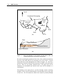
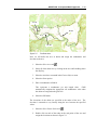
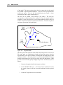
7.1 DESCRIPTION OF PROBLEM .....................................................................................................................7-1
7.2 GETTING STARTED ..................................................................................................................................7-3
7.3 REQUIRED MODULES/INTERFACES..........................................................................................................7-3
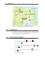
7.4 IMPORTING THE BACKGROUND IMAGE....................................................................................................7-3
7.4.1 Reading the Image.........................................................................................................................7-4
7.4.2 Image File vs. TIFF File ...............................................................................................................7-4
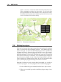
7.5 FEATURE OBJECTS ..................................................................................................................................7-4
7.6 BUILDING THE LOCAL SOURCE/SINK COVERAGE ....................................................................................7-5
7.6.1 Defining the Units .........................................................................................................................7-6
7.6.2 Defining the Boundary ..................................................................................................................7-6
7.6.3 Copying the Boundary...................................................................................................................7-7
7.6.4 Defining the Specified Head Arcs .................................................................................................7-8
7.6.5 Defining the Drain Arcs ..............................................................................................................7-10
7.6.6 Building the polygons..................................................................................................................7-12
7.6.7 Creating the Wells .......................................................................................................................7-13
7.7 DELINEATING THE RECHARGE ZONES ...................................................................................................7-14
7.7.1 Switching Coverages ...................................................................................................................7-14
7.7.2 Creating the Landfill Boundary ..................................................................................................7-14
7.7.3 Building the Polygons .................................................................................................................7-15
7.7.4 Assigning the Recharge Values ...................................................................................................7-15
7.8 DEFINING THE HYDRAULIC CONDUCTIVITY ..........................................................................................7-16
7.8.1 Top Layer ....................................................................................................................................7-16
7.8.2 Bottom Layer...............................................................................................................................7-16
7.9 LOCATING THE GRID FRAME .................................................................................................................7-17
7.10
CREATING THE GRID.........................................................................................................................7-18
7.11
DEFINING THE ACTIVE/INACTIVE ZONES ..........................................................................................7-18
7.12
INITIALIZING THE MODFLOW DATA...............................................................................................7-18
7.13
CONVERTING THE CONCEPTUAL MODEL ..........................................................................................7-19
7.14
INTERPOLATING LAYER ELEVATIONS ...............................................................................................7-19
7.14.1
Importing the Ground Surface Scatter Points.........................................................................7-20
7.14.2
Calculating a Starting Head Data Set ....................................................................................7-20
7.14.3
Interpolating the Heads and Elevations .................................................................................7-21
7.14.4
Importing the Layer Elevation Scatter Points.........................................................................7-21
Table of Contents
ix
7.14.5
Interpolating the Layer Elevations ......................................................................................... 7-21
7.14.6
Adjusting the Display.............................................................................................................. 7-22
7.14.7
Viewing the Model Cross Sections.......................................................................................... 7-22
7.14.8
Fixing the Elevation Arrays.................................................................................................... 7-23
7.15
CHECKING THE SIMULATION............................................................................................................. 7-23
7.16
SAVING THE PROJECT ....................................................................................................................... 7-24
7.17
RUNNING MODFLOW..................................................................................................................... 7-25
7.18
VIEWING THE HEAD CONTOURS ....................................................................................................... 7-25
7.19
VIEWING THE WATER TABLE IN SIDE VIEW...................................................................................... 7-25
7.20
VIEWING THE FLOW BUDGET ........................................................................................................... 7-26
7.21
ADDING ANNOTATION ...................................................................................................................... 7-27
7.22
CONCLUSION .................................................................................................................................... 7-28
8
MODPATH............................................................................................................................................... 8-1
8.1 DESCRIPTION OF PROBLEM ..................................................................................................................... 8-1
8.2 GETTING STARTED .................................................................................................................................. 8-2
8.3 REQUIRED MODULES/INTERFACES ......................................................................................................... 8-2
8.4 IMPORTING THE PROJECT ........................................................................................................................ 8-2
8.5 INITIALIZING THE MODPATH SIMULATION ........................................................................................... 8-2
8.6 ASSIGNING THE POROSITIES .................................................................................................................... 8-3
8.6.1 Assigning the Porosities to the Cells............................................................................................. 8-3
8.7 DEFINING THE STARTING LOCATIONS ..................................................................................................... 8-4
8.7.1 Selecting the Cell .......................................................................................................................... 8-4
8.7.2 Creating the Starting Locations .................................................................................................... 8-4
8.8 SPECIFYING THE TRACKING DIRECTION .................................................................................................. 8-5
8.9 SAVING THE SIMULATION ....................................................................................................................... 8-5
8.10
RUNNING MODPATH ....................................................................................................................... 8-5
8.11
VIEWING THE SOLUTION ..................................................................................................................... 8-6
8.11.1
Viewing the Pathlines in Cross Section View ........................................................................... 8-6
8.12
TRACKING PARTICLES FROM THE LANDFILL ....................................................................................... 8-6
8.12.1
Changing the Tracking Direction ............................................................................................. 8-6
8.12.2
Deleting the Starting Locations ................................................................................................ 8-7
8.12.3
Defining the New Starting Locations........................................................................................ 8-7
8.13
SAVING THE SIMULATION ................................................................................................................... 8-8
8.14
RUNNING MODPATH ....................................................................................................................... 8-8
8.15
VIEWING THE SOLUTION ..................................................................................................................... 8-8
8.16
CONCLUSION ...................................................................................................................................... 8-8
9
MT3DMS – GRID APPROACH............................................................................................................. 9-1
9.1 DESCRIPTION OF PROBLEM ..................................................................................................................... 9-1
9.2 GETTING STARTED .................................................................................................................................. 9-2
9.3 REQUIRED MODULES/INTERFACES ......................................................................................................... 9-2
9.4 BUILDING THE FLOW MODEL .................................................................................................................. 9-3
9.4.1 Creating the Grid .......................................................................................................................... 9-3
9.4.2 Initializing the MODFLOW Simulation ........................................................................................ 9-4
9.4.3 The Basic Package ........................................................................................................................ 9-4
9.4.4 The BCF Package ......................................................................................................................... 9-6
9.4.5 Defining the Wells ......................................................................................................................... 9-7
9.4.6 Saving the Simulation.................................................................................................................... 9-8
9.4.7 Running MODFLOW .................................................................................................................... 9-8
9.4.8 Viewing the Flow Solution ............................................................................................................ 9-8
9.5 BUILDING THE TRANSPORT MODEL ........................................................................................................ 9-9
9.5.1 Initializing the Simulation ............................................................................................................. 9-9
x
GMS Tutorials
9.5.2 The Basic Transport Package .......................................................................................................9-9
9.5.3 The Advection Package ...............................................................................................................9-11
9.5.4 The Dispersion Package..............................................................................................................9-11
9.5.5 The Source/Sink Mixing Package................................................................................................9-12
9.5.6 Saving the Simulation..................................................................................................................9-12
9.5.7 Running MT3DMS ......................................................................................................................9-13
9.5.8 Reading in the Transport Solution ..............................................................................................9-13
9.5.9 Changing the Contouring Options ..............................................................................................9-13
9.5.10
Setting Up a Film Loop...........................................................................................................9-13
9.6 CONCLUSION.........................................................................................................................................9-14
10
MT3DMS – CONCEPTUAL MODEL APPROACH .........................................................................10-1
10.1
DESCRIPTION OF PROBLEM ...............................................................................................................10-1
10.2
GETTING STARTED ...........................................................................................................................10-2
10.3
REQUIRED MODULES/INTERFACES ...................................................................................................10-2
10.4
IMPORTING THE PROJECT..................................................................................................................10-2
10.5
INITIALIZING THE MT3DMS SIMULATION ........................................................................................10-3
10.5.1
Defining the Units...................................................................................................................10-3
10.5.2
Defining the Species................................................................................................................10-3
10.5.3
Defining the Stress Periods.....................................................................................................10-3
10.5.4
Selecting Output Control ........................................................................................................10-4
10.5.5
Selecting the Packages............................................................................................................10-4
10.6
ASSIGNING THE AQUIFER PROPERTIES ..............................................................................................10-5
10.6.1
Assigning the Parameters to the Polygons .............................................................................10-5
10.7
ASSIGNING THE RECHARGE CONCENTRATION ..................................................................................10-6
10.8
CONVERTING THE CONCEPTUAL MODEL ..........................................................................................10-6
10.9
LAYER THICKNESSES........................................................................................................................10-6
10.10 THE ADVECTION PACKAGE ..............................................................................................................10-6
10.11 THE DISPERSION PACKAGE...............................................................................................................10-7
10.12 THE SOURCE/SINK MIXING PACKAGE DIALOG .................................................................................10-7
10.13 SAVING THE SIMULATION .................................................................................................................10-8
10.14 RUNNING MT3DMS......................................................................................................................... 10-8
10.15 VIEWING THE SOLUTION ...................................................................................................................10-8
10.16 VIEWING A FILM LOOP......................................................................................................................10-9
10.17 MODELING SORPTION AND DECAY .................................................................................................10-10
10.17.1 Turning on the Chemical Reactions Package .......................................................................10-10
10.17.2 Entering the Sorption and Biodegradation Data..................................................................10-10
10.18 SAVING THE SIMULATION ...............................................................................................................10-11
10.19 RUNNING MT3DMS.......................................................................................................................10-11
10.20 VIEWING THE SOLUTION .................................................................................................................10-11
10.21 GENERATING A TIME HISTORY PLOT ..............................................................................................10-12
10.21.1 Creating an Observation Coverage ......................................................................................10-12
10.21.2 Creating an Observation Point.............................................................................................10-12
10.21.3 Creating a Time Series Plot ..................................................................................................10-13
10.21.4 Plotting Multiple Curves.......................................................................................................10-13
10.21.5 Moving the Observation Point ..............................................................................................10-13
10.22 CONCLUSION ..................................................................................................................................10-14
11
SEAM3D .................................................................................................................................................11-1
11.1
11.2
11.3
11.4
DESCRIPTION OF PROBLEM ...............................................................................................................11-1
GETTING STARTED ...........................................................................................................................11-2
REQUIRED MODULES/INTERFACES ...................................................................................................11-2
IMPORTING THE FLOW MODEL .........................................................................................................11-3
Table of Contents
xi
11.5
INITIALIZING THE SEAM3D SIMULATION......................................................................................... 11-3
11.6
BASIC TRANSPORT PACKAGE ........................................................................................................... 11-3
11.6.1
Defining the Units................................................................................................................... 11-4
11.6.2
Setting up the Stress Periods .................................................................................................. 11-4
11.6.3
Package Selection................................................................................................................... 11-4
11.6.4
Defining the Species ............................................................................................................... 11-5
11.6.5
Output Control........................................................................................................................ 11-5
11.6.6
Entering the Porosity.............................................................................................................. 11-6
11.6.7
Starting Concentrations.......................................................................................................... 11-6
11.7
ADVECTION PACKAGE ...................................................................................................................... 11-7
11.8
DISPERSION PACKAGE ...................................................................................................................... 11-7
11.9
SOURCE/SINK MIXING PACKAGE ...................................................................................................... 11-7
11.10 CHEMICAL REACTION PACKAGE....................................................................................................... 11-8
11.11 NAPL DISSOLUTION PACKAGE ........................................................................................................ 11-9
11.11.1 Selecting the Cells................................................................................................................... 11-9
11.11.2 Assigning the Concentration................................................................................................. 11-10
11.11.3 Entering the NAPL Data....................................................................................................... 11-10
11.12 BIODEGRADATION PACKAGE .......................................................................................................... 11-11
11.12.1 Minimum Concentrations ..................................................................................................... 11-11
11.12.2 Electron Acceptor Coefficients ............................................................................................. 11-11
11.12.3 Generation Coefficients ........................................................................................................ 11-12
11.12.4 Use Coefficients .................................................................................................................... 11-12
11.12.5 Saturation Constants ............................................................................................................ 11-12
11.12.6 Rates ..................................................................................................................................... 11-13
11.12.7 Starting Concentrations........................................................................................................ 11-13
11.13 SAVING AND RUNNING THE SIMULATION ........................................................................................ 11-13
11.14 READING THE SOLUTION ................................................................................................................ 11-14
11.15 SETTING THE CONTOURING OPTIONS .............................................................................................. 11-14
11.16 VIEWING THE CONCENTRATION CONTOURS ................................................................................... 11-14
11.17 SETTING UP A TIME SERIES PLOT.................................................................................................... 11-15
11.17.1 Moving the Observation Point.............................................................................................. 11-16
11.17.2 Plotting Multiple Data Sets................................................................................................... 11-16
11.18 OTHER VIEWING OPTIONS .............................................................................................................. 11-17
11.19 CONCLUSION .................................................................................................................................. 11-17
12
DEFINING LAYER DATA................................................................................................................... 12-1
12.1
GETTING STARTED ........................................................................................................................... 12-1
12.2
REQUIRED MODULES/INTERFACES ................................................................................................... 12-1
12.3
USING THE "TRUE LAYER" MODE .................................................................................................... 12-2
12.4
INTERPOLATING TO MODFLOW LAYERS ........................................................................................ 12-2
12.5
SAMPLE PROBLEMS .......................................................................................................................... 12-3
12.6
BUILDING THE GRID ......................................................................................................................... 12-3
12.7
CASE 1 – COMPLETE LAYERS ........................................................................................................... 12-3
12.7.1
Importing the Scatter Point Sets ............................................................................................. 12-4
12.7.2
Interpolating the Elevation Values ......................................................................................... 12-5
12.7.3
Viewing the Results................................................................................................................. 12-5
12.8
CASE 2 – EMBEDDED SEAM ............................................................................................................. 12-6
12.8.1
Importing the Scatter Points ................................................................................................... 12-6
12.8.2
Interpolating the Values ......................................................................................................... 12-7
12.8.3
Correcting the Layer Data...................................................................................................... 12-7
12.9
CASE 3 – OUTCROPPING ................................................................................................................... 12-8
12.9.1
Importing the Points ............................................................................................................... 12-8
12.9.2
Interpolating the Values ......................................................................................................... 12-9
xii
GMS Tutorials
12.9.3
Correcting the Layer Values ...................................................................................................12-9
12.10 CASE 4 – BEDROCK TRUNCATION ..................................................................................................12-10
12.10.1 Importing the Scatter Points .................................................................................................12-10
12.10.2 Interpolating the Values........................................................................................................12-11
12.10.3 Viewing the Results ...............................................................................................................12-11
12.10.4 Correcting the Layer Values .................................................................................................12-11
12.10.5 Viewing the Corrected Layers...............................................................................................12-12
12.11 CONCLUSION ..................................................................................................................................12-12
13
REGIONAL TO LOCAL MODEL CONVERSION...........................................................................13-1
DESCRIPTION OF PROBLEM ............................................................................................................................13-1
13.1
GETTING STARTED ...........................................................................................................................13-3
13.2
REQUIRED MODULES/INTERFACES ...................................................................................................13-3
13.3
READING IN THE REGIONAL MODEL .................................................................................................13-3
13.4
CONVERTING THE LAYER DATA TO A SCATTER POINT SET...............................................................13-4
13.5
APPROACHES TO BUILDING THE LOCAL MODEL ...............................................................................13-4
13.6
BUILDING THE LOCAL CONCEPTUAL MODEL ....................................................................................13-5
13.6.1
Creating a New Coverage.......................................................................................................13-5
13.6.2
Creating the Boundary Arcs ...................................................................................................13-5
13.6.3
Building the Polygon ..............................................................................................................13-6
13.6.4
Marking the Specified Head Arcs ...........................................................................................13-7
13.7
CREATING THE LOCAL MODFLOW MODEL ....................................................................................13-7
13.7.1
Creating the Grid....................................................................................................................13-7
13.7.2
Activating the Cells .................................................................................................................13-8
13.7.3
Mapping the Attributes ...........................................................................................................13-8
13.8
INTERPOLATING THE LAYER DATA ...................................................................................................13-9
13.9
SAVING AND RUNNING THE LOCAL MODEL ......................................................................................13-9
13.10 VIEWING THE RESULTS .....................................................................................................................13-9
13.11 CONCLUSION ..................................................................................................................................13-10
14
MODEL CALIBRATION .....................................................................................................................14-1
14.1
DESCRIPTION OF PROBLEM ...............................................................................................................14-1
14.2
GETTING STARTED ...........................................................................................................................14-3
14.3
REQUIRED MODULES/INTERFACES ...................................................................................................14-3
14.4
READING IN THE MODEL...................................................................................................................14-4
14.5
OBSERVATION DATA ........................................................................................................................14-4
14.6
ENTERING OBSERVATION POINTS .....................................................................................................14-4
14.6.1
Creating an Observation Coverage ........................................................................................14-4
14.6.2
Creating an Observation Point...............................................................................................14-5
14.6.3
Calibration Target ..................................................................................................................14-6
14.6.4
Point Statistics ........................................................................................................................14-7
14.7
READING IN A SET OF OBSERVATION POINTS ....................................................................................14-7
14.7.1
Deleting the Current Coverage...............................................................................................14-7
14.7.2
Reading in the Points..............................................................................................................14-8
14.8
ENTERING THE OBSERVED STREAM FLUX ........................................................................................14-8
14.9
GENERATING ERROR PLOTS .............................................................................................................14-9
14.9.1
Computed vs. Observed Plot.................................................................................................14-10
14.9.2
Error Summary .....................................................................................................................14-10
14.10 EDITING THE HYDRAULIC CONDUCTIVITY ......................................................................................14-10
14.11 CONVERTING THE MODEL ..............................................................................................................14-11
14.12 COMPUTING A SOLUTION ................................................................................................................14-12
14.12.1 Saving the Simulation ...........................................................................................................14-12
14.12.2 Running MODFLOW ............................................................................................................14-12
Table of Contents
xiii
14.13 READING IN THE SOLUTION ............................................................................................................ 14-12
14.14 ERROR VS. SIMULATION PLOT ........................................................................................................ 14-13
14.15 CONTINUING THE TRIAL AND ERROR CALIBRATION ....................................................................... 14-13
14.15.1 Changing Values vs. Changing Zones .................................................................................. 14-13
14.15.2 Viewing the Answer .............................................................................................................. 14-14
14.16 CONCLUSION .................................................................................................................................. 14-14
15
FEMWATER – FLOW MODEL.......................................................................................................... 15-1
15.1
DESCRIPTION OF PROBLEM ............................................................................................................... 15-1
15.2
GETTING STARTED ........................................................................................................................... 15-2
15.3
REQUIRED MODULES/INTERFACES ................................................................................................... 15-2
15.4
BUILDING THE CONCEPTUAL MODEL ............................................................................................... 15-3
15.4.1
Importing the Background Image........................................................................................... 15-3
15.4.2
Initializing the FEMWATER Coverage................................................................................... 15-3
15.4.3
Defining the Units................................................................................................................... 15-4
15.4.4
Creating the Boundary Arcs ................................................................................................... 15-4
15.4.5
Redistributing the Arc Vertices............................................................................................... 15-4
15.4.6
Defining the Boundary Conditions ......................................................................................... 15-5
15.4.7
Building the Polygon .............................................................................................................. 15-5
15.4.8
Assigning the Recharge .......................................................................................................... 15-6
15.4.9
Creating the Wells .................................................................................................................. 15-6
15.5
BUILDING THE 3D MESH .................................................................................................................. 15-7
15.5.1
Defining the Materials ............................................................................................................ 15-8
15.5.2
Building the 2D Projection Mesh ........................................................................................... 15-8
15.5.3
Building the TINs.................................................................................................................... 15-8
15.5.4
Importing and Interpolating the Terrain Data ....................................................................... 15-9
15.5.5
Importing and Interpolating the Layer Elevation Data ........................................................ 15-10
15.5.6
Building the 3D Mesh ........................................................................................................... 15-12
15.6
HIDING OBJECTS ............................................................................................................................ 15-13
15.7
CONVERTING THE CONCEPTUAL MODEL ........................................................................................ 15-14
15.8
SELECTING THE ANALYSIS OPTIONS ............................................................................................... 15-14
15.8.1
Entering the Run Options ..................................................................................................... 15-14
15.8.2
Setting the Iteration Parameters........................................................................................... 15-15
15.8.3
Selecting Output Control ...................................................................................................... 15-15
15.8.4
Defining the Fluid Properties ............................................................................................... 15-15
15.9
DEFINING INITIAL CONDITIONS ....................................................................................................... 15-16
15.9.1
Creating the Scatter Point Set .............................................................................................. 15-16
15.9.2
Creating the Data Set ........................................................................................................... 15-18
15.10 DEFINING THE MATERIAL PROPERTIES ........................................................................................... 15-18
15.11 SAVING AND RUNNING THE MODEL................................................................................................ 15-19
15.12 VIEWING THE SOLUTION ................................................................................................................. 15-20
15.12.1 Viewing Fringes.................................................................................................................... 15-20
15.12.2 Viewing a Water Table Iso-Surface ...................................................................................... 15-20
15.12.3 Draping the TIFF Image on the Ground Surface ................................................................. 15-21
15.13 CONCLUSION .................................................................................................................................. 15-22
16
SEEP2D - CONFINED .......................................................................................................................... 16-1
16.1
DESCRIPTION OF PROBLEM ............................................................................................................... 16-1
16.2
GETTING STARTED ........................................................................................................................... 16-2
16.3
REQUIRED MODULES/INTERFACES ................................................................................................... 16-2
16.4
CREATING THE MESH ....................................................................................................................... 16-3
16.4.1
Defining a Coordinate System ................................................................................................ 16-3
16.4.2
Creating the Corner Nodes..................................................................................................... 16-4
xiv
GMS Tutorials
16.4.3
Interpolating Intermediate Nodes ...........................................................................................16-5
16.4.4
Creating an Extra Node ..........................................................................................................16-6
16.4.5
Creating the Elements.............................................................................................................16-6
16.4.6
Deleting the Sheet Pile Element..............................................................................................16-7
16.4.7
Refining the Mesh ...................................................................................................................16-8
16.5
RENUMBERING THE MESH ................................................................................................................16-9
16.6
INITIALIZING THE SEEP2D SOLUTION ............................................................................................16-10
16.7
SETTING THE ANALYSIS OPTIONS ...................................................................................................16-10
16.8
ASSIGNING MATERIAL PROPERTIES ................................................................................................16-11
16.9
ASSIGNING BOUNDARY CONDITIONS ..............................................................................................16-12
16.9.1
Constant Head Boundaries ...................................................................................................16-12
16.10 SAVING THE SIMULATION ...............................................................................................................16-13
16.11 RUNNING SEEP2D ......................................................................................................................... 16-14
16.12 VIEWING THE SOLUTION .................................................................................................................16-14
16.13 CONCLUSION ..................................................................................................................................16-14
17
SEEP2D - UNCONFINED.....................................................................................................................17-1
17.1
DESCRIPTION OF PROBLEM ...............................................................................................................17-1
17.2
GETTING STARTED ...........................................................................................................................17-2
17.3
REQUIRED MODULES/INTERFACES ...................................................................................................17-2
17.4
CREATING THE MESH .......................................................................................................................17-2
17.4.1
Defining a Coordinate System ................................................................................................17-3
17.4.2
Creating a Coverage...............................................................................................................17-4
17.4.3
Creating the Corner Points.....................................................................................................17-4
17.4.4
Creating the Arcs ....................................................................................................................17-5
17.4.5
Redistributing Vertices............................................................................................................17-6
17.4.6
Creating the Polygons ............................................................................................................17-6
17.4.7
Assigning the Material Types..................................................................................................17-6
17.4.8
Constructing the Mesh ............................................................................................................17-7
17.5
RENUMBERING THE MESH ................................................................................................................17-7
17.6
INITIALIZING THE SEEP2D SOLUTION ..............................................................................................17-8
17.7
SETTING THE ANALYSIS OPTIONS .....................................................................................................17-8
17.8
ASSIGNING MATERIAL PROPERTIES ..................................................................................................17-8
17.9
ASSIGNING BOUNDARY CONDITIONS ................................................................................................17-9
17.9.1
Specified Head Boundary Conditions.....................................................................................17-9
17.9.2
Exit Face Boundary Conditions............................................................................................ 17-10
17.10 SAVING THE SIMULATION ...............................................................................................................17-10
17.11 RUNNING SEEP2D ......................................................................................................................... 17-11
17.12 VIEWING THE SOLUTION .................................................................................................................17-11
17.13 MODELING FLOW IN THE UNSATURATED ZONE ..............................................................................17-12
17.13.1 Reading in the Original Model .............................................................................................17-12
17.13.2 Changing the Mesh Display..................................................................................................17-12
17.13.3 Changing the Analysis Options.............................................................................................17-12
17.13.4 Editing the Material Properties ............................................................................................17-13
17.14 SAVING THE SIMULATION ...............................................................................................................17-13
17.15 RUNNING SEEP2D ......................................................................................................................... 17-14
17.16 VIEWING THE SOLUTION .................................................................................................................17-14
17.17 CONCLUSION ..................................................................................................................................17-15
1
Introduction
CHAPTER
1
Introduction
This document contains tutorials for the Department of Defense Groundwater
Modeling System (GMS). Each tutorial provides training on a specific
component of GMS. Since the GMS interface contains a large number of
options and commands, you are strongly encouraged to complete the tutorials
before attempting to use GMS on a routine basis.
In addition to this document, the GMS Reference Manual also describes the
GMS interface. Typically, the most effective approach to learning GMS is to
complete the tutorials before reading the reference manual.
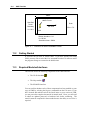
1.1
Suggested Order Of Completion
In most cases, the tutorials can be completed in any desired order. However,
some of the tutorials are pre-requisites for other tutorials. For example, since
TINs are used in the construction of solid models, the Surface Modeling With
TINs tutorial (Chapter 2) should be completed before the Stratigraphy
Modeling With Solids tutorial (Chapter 3).
1.2
RT3D Tutorials
This document contains all of the tutorials for GMS except for the RT3D
tutorials. Due to the large number of RT3D tutorials (one for each reaction
package), they are contained in a separate document.
1-2
1.3
GMS Tutorials
Demo vs. Normal Mode
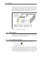
The interface for GMS is divided into ten modules. Some of the modules
contain interfaces to models such as MODFLOW. Such interfaces are
typically contained within a single menu. Since some users may not require
all of the modules or model interfaces provided in GMS, modules and model
interfaces can be licensed individually. Modules and interfaces that have been
licensed are enabled using the Register command in the File menu. The icons
for the unlicensed modules or the menus for model interfaces are dimmed and
cannot be accessed.
GMS provides two modes of operation: demo and normal. In normal mode,
the modules and interfaces you have licensed are undimmed and fully
functional and the items you have not licensed are dimmed and inaccessible.
In demo mode, all modules and interfaces are undimmed and functional
regardless of which items have been licensed. However, all of the print and
save commands are disabled.
While some of the tutorials may be completed in either normal or demo mode,
many of them can only be completed in normal mode. The required mode is
discussed at the beginning of each tutorial. If the tutorial must be completed
in normal mode, the modules and interfaces needed for the tutorial are listed.
If some of the required items have not been licensed, you will need to obtain
an updated password or hardware lock before you complete the tutorial.
2
Surface Modeling With TINs
CHAPTER
2
Surface Modeling With TINs
The TIN module in GMS is used for general-purpose surface modeling. TINs
are formed by connecting a set of xyz points (scattered or gridded) with edges
to form a network of triangles. The surface is assumed to vary linearly across
each triangle. TINs can be used to represent the surface of a geologic unit or
the surface defined by a mathematical function. TINs can be displayed in
oblique view with hidden surfaces removed. Elevations or other values
associated with TINs can be displayed with color fringes or contours. TINs
are used in the construction of solid models and 3D finite element meshes.
This tutorial should be completed before beginning the Stratigraphy Modeling
with Solids tutorial. The emphasis in this tutorial is on the basic tools for
editing TINs. A description of how TINs are used in the construction of solids
is provided in the following tutorial.
2.1
Getting Started
If you have not yet done so, launch GMS. If you have already been using
GMS, you may wish to select the New command from the File menu to ensure
the program settings are restored to the default state.
2.2
Required Modules/Interfaces
This tutorial can be completed in either demo mode or normal model. If you
are already in demo mode, you may continue with the tutorial. If you are in
normal mode, you will need to ensure that the necessary components have
2-2
GMS Tutorials
been licensed. This tutorial utilizes the following components of the GMS
interface:
•
The TIN module
•
The 2D Scatter Point module
You can confirm whether each of these components has been enabled on your
copy of GMS by selecting the Register command from the File menu. If each
of these items is enabled, you can proceed to complete the tutorial in normal
mode. If not, you will need to switch to demo mode before continuing. To
switch to demo mode:
1. Select the Demo Mode command from the File menu.
2. Select OK at the prompts.
2.3
Importing Vertices
To begin reviewing the tools available for TIN modeling, we will first import a
set of vertices from a text file. These vertices are simply a set of xyz points
entered into a TIN file. The TIN file format is described in the GMS File
Format document.
To import the vertices:
1. If necessary, switch to the TIN module
.
2. Select the Open command from the File menu.
3. At the bottom of the Open dialog, select the *.tin filter.
4. In the Read File dialog, locate and open the directory entitled
tutorial\tins.
5. Select the file entitled verts.tin.
6. Select the Open button.
A set of points should appear on the screen.
Surface Modeling With TINs
2.4
2-3
Triangulating
To construct a TIN, we must triangulate the set of vertices we have imported.
To triangulate the points:
Select the Triangulate command from the Build TIN menu.
The vertices should now be connected with edges forming a network of
triangles. The triangulation is performed automatically using the Delauney
criterion. The Delauney criterion ensures that the triangles are as "equiangular" as possible. In other words, wherever possible, long thin triangles are
avoided. A more complete description of the triangulation algorithm can be
found in Chapter 4 of the GMS Reference Manual.
2.5
Contouring
Now that the TIN is constructed, we can use it to generate a contour plot of the
TIN elevations.
.
1. Select the Display Options macro
2. Turn on the Contours and TIN Boundary options and turn off the
Triangles and Vertices options.
3. Select the OK button.
The contours are generated by assuming that the TIN defines a surface that
varies linearly across the face of each triangle.
2.6
Shading
Another way to visualize a TIN is to shade the TIN.
.
1. Select the Display Options macro
2. Turn off the Contours and TIN Boundary options and turn on the
Triangles option.
3. Select the OK button.
4. Select the Oblique View macro
5. Select the Shade macro
.
.
2-4
2.7
GMS Tutorials
Editing TINs
As TINs are used in the construction of solids and meshes, it is usually
necessary to edit a TIN once it has been created. In many cases, TINs are
constructed from a sparse set of points and it is necessary to "fill in the gaps"
between the vertices and "sculpt" the TIN using the editing tools to ensure that
the TIN is a reasonable representation of the surface being modeled.
A variety of tools are provided in GMS for editing TINs. Before reviewing
these tools, we will reset some of the display options.
1. Select the Display Options macro
.
2. Turn on the Vertices and Contours options.
3. Select the Options button to the right of the Contours option.
4. In the section titled Contour Interval, select the Specified Interval
option and change the interval to 20.0.
5. Select the OK button to exit the Contour Options dialog.
6. Select the Close button to exit the TIN Display Options dialog.
2.8
Dragging Vertices
One of the simplest ways to edit a TIN is to drag the vertices with the cursor.
This can be accomplished with the Select Vertices tool.
from the Tool Palette.
1. Choose the Select Vertices tool
2. Select the Plan View macro
.
3. Choose one of the vertices in the interior of the TIN and drag it to a
new location.
Notice that as you move the vertex, the contours of the TIN are
instantaneously updated to give you visual feedback on the changes that you
are making. You may have also noticed that you are not allowed to drag an
interior vertex beyond the boundaries of the adjacent triangles. This prevents
the triangles from becoming inverted.
Surface Modeling With TINs
2.9
2-5
Dragging in Oblique View
When dragging in plan view, the vertex is constrained to move in the xy plane.
To change the z coordinate, we must drag the vertices in oblique view (or front
or side view).
1. Select the Oblique View macro
.
2. Select one of the vertices and drag the vertex up and down.
Notice that as you drag the vertex in oblique view, you are constrained to
move the vertex along the z axis.
2.10
Using the Edit Window
In many cases, dragging vertices with the mouse is not adequately precise. It
is often necessary to change the vertex coordinates to a specific value. This
type of editing can be accomplished with the input fields at the top of the GMS
window.
Choose one of the vertices in the TIN and select it by clicking on it
with the cursor.
Notice that as the vertex is selected, the coordinates of the vertex are displayed
in the fields at the top of the window. The edit fields can be used to change
the x, y, or z coordinates of the selected vertex.
1. Move the cursor to the z coordinate field and add a value of 5.0 to the
current z value of the vertex.
2. Hit the Return or Tab key.
Again, as the vertex coordinates change, the triangle edges and contours of the
surface are immediately updated.
2.11
Locking Vertices
In many cases, some of the vertices defining a TIN come from actual
measured data such as a borehole log and can be considered "hard" data. In
other cases, vertices are added manually and represent "soft" data used simply
to fill in gaps. When editing a TIN, it is useful to distinguish between these
two types of vertices so that a vertex corresponding to an actual measurement
is not accidentally edited. This can be accomplished by "locking" and
"unlocking" vertices.
2-6
GMS Tutorials
1. Select several vertices by dragging a box around the vertices or by
clicking on individual vertices while holding down the Shift key.
2. Select the Lock/Unlock Vertices command from the Modify TIN menu.
Notice that the color of the vertices changes when they are locked. Once a set
of vertices is locked, the coordinates of the vertices cannot be changed.
1. Click once outside the TIN to unselect the vertices.
2. Select one of the vertices that you just locked.
3. Attempt to edit the vertex by dragging or by entering new coordinates
in the Edit Window.
Locked vertices can be unlocked by selecting the vertices and selecting the
Lock/Unlock Vertices command from the Modify TIN menu.
2.12
Adding Vertices
As mentioned above, when working with TINs it is often necessary to edit a
TIN by adding supplemental vertices to the TIN to provide more resolution or
detail in an area of interest. Vertices can be added to a TIN in GMS simply by
pointing and clicking.
1. Select the Plan View macro
2. Select the Create Vertex
.
tool.
3. Place the cursor in the interior of one of the triangles in the TIN and
create a vertex by clicking the mouse button.
A dialog appears prompting for the z value of the new vertex. The default
value is computed using a linear interpolation of the surrounding vertices.
Select the OK button to accept the default value.
Notice that the vertex was automatically incorporated into the TIN topology.
In addition, the vertex is selected and can be edited using the edit fields in the
Edit Window.
2.13
Deleting Vertices
It is also frequently necessary to delete vertices. To delete the vertex you just
created:
Surface Modeling With TINs
2-7
1. Select the Delete command from the Edit menu.
2. Select OK to confirm the deletion.
Notice that all of the triangles connected to the vertex were deleted. By
default, this is what happens when a vertex is deleted. The resulting void can
be filled with triangles by using the Create Triangle tool to manually create
triangles. However, another option is available for deletion that causes the
region surrounding a deleted vertex to be automatically retriangulated.
1. Select the Vertex Options command from the Modify TIN menu.
2. Turn on the option entitled Retriangulate after deleting.
3. Select the OK button.
4. Choose the Select Vertices tool
.
5. Select one the vertices in the interior of the TIN.
6. Select the Delete command from the Edit menu.
7. Select OK to confirm the deletion.
Notice that the triangles next to the deleted vertex are deleted but the resulting
void is retriangulated.
2.14
Smoothing a TIN
As mentioned above, a TIN represents a piecewise linear surface. If the
vertices defining the TIN are sparse, the linear surface defined by the triangles
may appear excessively irregular. A TIN can be smoothed in GMS by copying
the TIN vertices to a scatter point set, subdividing the TIN into a denser set of
triangles, and interpolating the elevations to the new vertices in the TIN. The
resulting TIN is still piecewise linear but it appears much smoother since the
triangles are smaller.
2.14.1 Deleting the TIN
We will now go through an example of TIN smoothing, but first we will read
in a different TIN since we have made several changes to this TIN.
1. Select the Delete All command from the Edit menu.
2. Select OK to confirm the deletion.
2-8
GMS Tutorials
3. Select the Open command from the File menu.
4. Select No at the prompt about saving the project.
5. In the Open dialog, select the *.tin filter.
6. Select the file entitled "sparse.tin".
7. Click on the Open button.
2.14.2 Copying the Vertices
The first step in smoothing the TIN is to copy the vertices of the TIN to a
scatter point set. This will allow us to use the scatter point set later to
interpolate the z values of the original vertices to the new vertices created
while subdividing the TIN.
1. Select the TIN -> Scatter Points command in the Build TIN menu.
2. Select the OK button to accept the default name of the new scatter
point set.
3. Select the No button to indicate that you do not want to delete the
existing TIN.
2.14.3 Subdividing the TIN
The next step is to increase the resolution of the TIN by uniformly subdividing
the TIN.
1. Select the Uniformly Subdivide TIN command from the Modify TIN
menu.
2. Move the scroll bar to select a subdivision factor of 8.
3. Select the OK button.
2.14.4 Interpolating the Elevations
Notice that the contours of the TIN have not changed. There are more
triangles in the TIN but they still define essentially the same surface. To
smooth the TIN we must use one of the interpolation schemes and interpolate
from the original vertices of the TIN to the new vertices created during the
subdivision process.
1. Switch to the 2D Scatter Point module
.
Surface Modeling With TINs
2-9
2. Select the to Active TIN command from the Interpolation menu (we
will use the default interpolation method).
3. Enter a name of "new_elev" for the new data set.
4. Turn on the Map elevations option. This ensures that the data set
created on the TIN will be used to define the elevations of the TIN
vertices.
5. Select the OK button.
The contours on the TIN now appear smoother. To better view the variation in
the surface:
Select the Oblique View macro
.
2.14.5 Deleting the Scatter Point Set
The TIN smoothing process is now completed. Since we no longer need the
scatter point set, we will delete it.
1. Select the Delete All command from the Edit menu.
2. Select the OK button to confirm the deletion.
2.15
Reading Another TIN
In GMS, several TINs can be modeled at once. For example, we will now read
in another TIN without first deleting the existing TIN.
1. Switch to the TINs module
.
2. Select the Open command from the File menu.
3. Select No at the prompt about saving the project.
4. In the Open dialog, select the *.tin filter.
5. Select the file entitled "surface.tin".
6. Click on the Open button.
You should now see two TINs displayed at once.
2-10
GMS Tutorials
2.16
Changing the Active TIN
Whenever multiple TINs are being modeled, one of the TINs is designated as
the active TIN. Only the active TIN can be edited. A TIN can be designated
as the active TIN using the combo box at the top of the GMS window.
1. Choose the Select TINs tool
.
2. In the combo box titled "TIN", select the "sparse" item.
Notice that triangular shaped icons appear at the center of each TIN. A TIN is
selected by selecting the TIN icon. The active TIN has a letter "A" displayed
in the center of the icon. A TIN can also be designated as the active TIN by
double clicking on the TIN icon. For example:
Double click on the TIN icon entitled "surface".
The letter "A" is now displayed in the icon for the TIN we just read from a
file. This TIN can now be edited.
2.17
Hiding and Showing TINs
When multiple TINs are in memory, it is sometimes useful to hide some of the
TINs temporarily. This makes the display less cluttered and makes it easier to
edit or visualize an individual TIN. For example:
1. Select the TIN entitled "sparse" by clicking once on the TIN icon.
2. Select the Hide macro
2.18
from the Tool Palette.
Deleting the TINs
Since we are now finished with the TINs, we will delete them.
1. Select the New command from the File menu.
2. Select the No button to confirm the deletion.
2.19
Conclusion
This concludes the Surface Modeling With TINs tutorial. Now that you have
finished this tutorial and understand the basics of TIN modeling, you are
Surface Modeling With TINs
2-11
prepared to proceed to the tutorial entitled Stratigraphy Modeling with Solids
(Chapter 3).
If you were originally running in normal mode and switched to demo mode to
complete this tutorial, you can switch back to normal mode as follows:
1. Select the Normal Mode command from the File menu.
2. Select the OK button at the prompt.
If you wish to exit GMS at this time:
1. Select the Exit command from the File menu.
2. Select No at the prompt.
3
Stratigraphy Modeling With Solids
CHAPTER
3
Stratigraphy Modeling With Solids
The Solid module of GMS is used to construct three-dimensional models of
stratigraphy. Once such a model is created, cross sections can be cut anywhere
on the model and hidden surface removal and shading can be used to generate
highly realistic images of either the cross sections or the solids. Volumes of
solids can also be computed.
In this tutorial you will learn how to construct a set of solid models
representing soil stratigraphy using borehole data as input. Since TINs are
used in the construction of solids, you should first complete the tutorial
entitled Surface Modeling with TINs (Chapter 2) before beginning this tutorial.
It is also helpful if you read the introduction to the chapter describing the Solid
module in the GMS Reference Manual. This will give you a basic
understanding of the approach used to construct solid models.
3.1
Getting Started
If you have not yet done so, launch GMS. If you have already been using
GMS, you may wish to select the New command from the File menu to ensure
the program settings are restored to the default state.
3.2
Required Modules/Interfaces
This tutorial can be completed in either demo mode or normal model. If you
are already in demo mode, you may continue with the tutorial. If you are in
normal mode, you will need to ensure that the necessary components have
3-2
GMS Tutorials
been licensed. This tutorial utilizes the following components of the GMS
interface:
•
The TIN module
•
The Borehole module
•
The Solid module
•
The Map module
You can confirm whether each of these components has been enabled on your
copy of GMS by selecting the Register command from the File menu. If each
of these items is enabled, you can proceed to complete the tutorial in normal
mode. If not, you will need to switch to demo mode before continuing. To
switch to demo mode:
1. Select the Demo Mode command from the File menu.
2. Select OK at the prompts.
3.3
Constructing the Solid Models
Constructing a set of solid models of soil stratigraphy in GMS is a three step
process. In the first step, a set of boreholes is input. In the next step, a set of
surfaces (TINs) is constructed through contacts on the boreholes which are
selected by the user. These surfaces represent the interfaces between adjacent
soil layers. In the third step, the surfaces are used to construct solid models of
the soil layers.
3.4
Reading Borehole Data
The first step in the construction of the solid models is to import a set of
borehole logs. Borehole data can be entered one of two ways. The data can be
entered into a text file in the GMS borehole file format described in the GMS
Reference Manual. Alternately, the boreholes can be entered one at a time
using the Borehole Editor command in the Boreholes menu. In the interest of
time, we will use the first approach and import a set of boreholes from a
previously prepared borehole file. The borehole data in this file were obtained
from an actual site investigation.
To read in the file:
Stratigraphy Modeling With Solids
1. Switch to the Borehole module
3-3
.
2. Select the Open command from the File menu.
3. Locate and open the directory entitled tutorial\solids.
4. Select the file entitled holes.gpr.
5. Click on the Open button.
You should now see a 3D view of the borehole logs. Each of the colors
represents a different type of soil. The green soil is a clean sand, the red soil is
a silty sand, and the blue soil is a silty clayey fine sand. For the remainder of
this tutorial, the soils will be referred to by their colors for simplicity.
3.5
Changing the Z Scale
In some cases, it is useful to magnify the display in the z dimension so that the
variation in the stratigraphy depicted by the borehole logs is more apparent.
To change the z scale:
1. Select the Z Magnification command from the View menu.
2. Enter a value of 2.0.
3. Select the OK button.
The holes should now appear "stretched" in the vertical direction.
3.6
Displaying the Hole Names
To help distinguish between the holes on the screen throughout the remainder
of the tutorial, the names of the holes will be posted on the holes.
1. Select the Display Options macro
.
2. Turn on the Hole Names option.
3. Select the OK button.
The names of the holes should appear at the tops of the holes. These names
were defined in the borehole file.
3-4
3.7
GMS Tutorials
Creating an Extrapolation Polygon
The next step in the construction of the stratigraphy model is to create a set of
TINs that represent the interfaces between the soil layers depicted in the
borehole data. However, before constructing the TINs, we must first define an
extrapolation polygon. The extrapolation polygon defines the boundary or the
limits of the stratigraphy model. In many cases, the polygon corresponds to a
property boundary.
3.7.1
Setting Up the View
The extrapolation polygon will just enclose the boreholes. The polygon will
be entered in plan view.
Select the Plan View macro
.
To allow plenty of screen space to enter the polygon we will increase the
viewing area (zoom out).
1. Select the Zoom tool
.
2. While holding down the Shift key, click somewhere in the center of
the boreholes.
3.7.2
Turning on the Drawing Grid
We will be entering the extrapolation polygon interactively using the mouse.
To help guide the placement of the polygon, we will temporarily turn on a
drawing grid.
1. Select the Drawing Grid Options command from the Display menu.
2. Set the Spacing to 50.0.
3. Turn on the Snap to grid option.
4. Turn on the Display grid lines option.
5. Set the Grid line spacing increment to 1.
6. Select the OK button.
You should see a grid appear on the screen. Notice that as you move the
cursor across the Graphics Window, the coordinates that appear in the Edit
Window at the bottom of the screen move in increments of 50.
Stratigraphy Modeling With Solids
3.7.3
3-5
Defining the Boundary Arc
We are now ready to enter the extrapolation polygon. The extrapolation
polygon is entered using the feature object tools in the Map module. First, we
will create a single arc defining a closed loop around the site.
1. Switch to the Map module
.
2. Select the Create Arc tool
.
3. Create a single arc by clicking on the points shown in Figure 3.1
(clockwise or counter-clockwise - it does not matter). To ensure you
are placing the points in the proper location, note the cursor
coordinates displayed on the left side of the Edit Window. Begin with
the point (50, 700). To close the polygon, double click on the point
you started with.
(50, 700)
(250, 700)
2G
7G
1G
5G
(600, 400)
6G
4G
8G
3G
(50, 50)
Figure 3.1
3.7.4
(600, 50)
The Coordinates of the Points Defining the Extrapolation
Polygon.
Creating the Polygon
Now that we have created the arc, we must use the arc to build a polygon.
1. Select the Build Polygons command from the Feature Objects menu.
2. Select OK at the prompt to use all arcs.
3-6
GMS Tutorials
The Build Polygons command traverses the set of currently defined arcs and
makes polygons out of all of the closed loops found. This is trivial in this case
since there is only one arc and one closed loop.
3.7.5
Turning off the Drawing Grid
Now that the polygon is entered, you can turn off the drawing grid.
1. Select the Drawing Grid Options command from the Display menu.
2. Turn off the Snap to grid option.
3. Turn off the Display grid lines option.
4. Select the OK button.
5. Select the Oblique View macro
3.8
.
Constructing the Ground Surface TIN
You are now ready to construct a TIN using the borehole logs. We will begin
by constructing a TIN representing the ground surface. This TIN will pass
through the top of each of the boreholes.
3.8.1
Selecting the Contacts
Before constructing the TIN, you must first select the contacts (locations on
the boreholes) that will be used to create the TIN.
1. Switch to the Borehole module
2. Choose the Select Contacts tool
.
.
3. While holding the Shift key, click on the top of each of the holes.
3.8.2
Creating the TIN
Now that you have selected the points on the boreholes where the TIN is to
pass through, you can construct the TIN by triangulating the points.
1. Select the Contacts -> TIN command from the Boreholes menu.
2. Select the Auto-extrapolate only option.
Stratigraphy Modeling With Solids
3-7
3. Select the OK button.
4. Enter "topblue1" for the name of the TIN.
5. Select the OK button.
A blue TIN should appear. Note that the TIN passes through the borehole
contacts that were selected and it also extends out to the extrapolation
polygon. This TIN could now be edited, if desired, using the TIN editing tools
described in the previous tutorial to smooth or reshape the TIN. For the
purposes of this tutorial, the TIN is adequate as is and will not be edited.
3.8.3
Hiding the TIN
Before continuing, it is useful to hide the TIN so that it will not be cluttering
the display while the other TINs are being constructed. To hide the TIN:
.
1. Switch to the TIN module
2. Choose the Select TINs
tool.
3. Select the TIN you just created by clicking on its icon.
4. Select the Hide macro
.
5. Switch back to the Borehole module
3.9
.
Constructing the Green Seam TIN
Next, we will construct the TIN representing the top of the green seam that
cuts through the side. To select the contacts:
1. Choose the Select Contacts tool
.
2. Select the blue/green contact on hole 3G.
3.9.1
Automatically Selecting Contacts
We could now select the remaining contacts one at a time with the Shift key
down as we did last time. However, this time we will use the Auto Select
command to select the remaining holes. The Auto Select command is used to
select a set of contacts that match a previously selected contact.
1. Select the Auto Select command from the Boreholes menu.
3-8
GMS Tutorials
2. Select the OK button.
3.9.2
Creating the TIN
All of the contacts at the top of the green soil should now be selected. To
construct the TIN:
1. Select the Contacts -> TIN command from the Borehole menu.
2. Select the Auto-extrapolate with trimming to selected boreholes
option.
3. Select the OK button.
4. Enter "topgreen" for the name of the TIN.
5. Select the OK button.
A green TIN should appear. Note that once again the TIN is automatically
extended to the extrapolation polygon and in addition, the TIN is automatically
extended to a point halfway between the holes that were selected and the holes
that were not selected. Of course, this boundary could be edited, but it
provides a reasonable initial estimate of the extent of the surface defined by
the selected contacts. For the purposes of this tutorial, we will accept the
default surface.
3.9.3
Hiding the TIN
To hide the TIN:
.
1. Switch to the TIN module
2. Choose the Select TINs
tool.
3. Select the TIN you just created by clicking on its icon.
4. Select the Hide macro
.
5. Switch back to the Borehole module
3.10
.
Constructing the Red Soil TIN
Next, we will construct the TIN representing the top of the red soil unit at the
lower part of the stratigraphy.
Stratigraphy Modeling With Solids
3-9
3.10.1 Constructing the TIN
To construct the TIN:
.
1. Choose the Select Contacts tool
2. Select the blue/red contact on hole 4G.
3. Select the Auto Select command from the Boreholes menu.
4. Turn off the Match material above option.
5. Select the OK button.
6. Select the Contacts -> TIN command from the Boreholes menu.
7. Select the Auto-extrapolate only option.
8. Select the OK button.
9. Enter "topred" for the name of the TIN.
10. Select the OK button.
3.10.2 Hiding the TIN
To hide the TIN:
.
1. Switch to the TIN module
2. Choose the Select TINs tool
.
3. Select the TIN you just created by clicking on its icon.
4. Select the Hide macro
.
5. Switch back to the Borehole module
3.11
.
Constructing the Blue Seam TINs
Most of the boreholes show a thin region of blue soil near the bottom of the
holes. We will model this region as a blue seam which cuts diagonally
through the site. This seam will lie entirely within the red soil. To model the
seam, we will need to construct two TINs: one at the top of the seam and one
at the bottom.
3-10
GMS Tutorials
3.11.1 Constructing the Top TIN
To construct the TIN at the top of the seam:
1. Choose the Select Contacts tool
.
2. Select the red/blue contact on hole 8G (see Figure 3.2).
3. Select the Auto Select command from the Boreholes menu.
4. Select the OK button.
5. Select the Contacts -> TIN command from the Boreholes menu.
6. Select the Auto-extrapolate with trimming to selected boreholes
option.
7. Select the OK button.
8. Enter "topblue2" for the name of the TIN.
9. Select the OK button.
8G
Select this contact
Figure 3.2
Contact on Hole 8G to be Selected.
3.11.2 Constructing the Bottom TIN
To construct the TIN at the bottom of the seam.
Stratigraphy Modeling With Solids
3-11
1. Since the Auto Select command will not work in this case, hold down
the Shift key and select the following contacts (see Figure 3.3):
the lower blue/red contact on hole 8G.
the bottom of hole 6G,
the blue/red contact on hole 7G,
the lower blue/red contact on hole 5G,
and the bottom of hole 2G.
2. Select the Contacts -> TIN command from the Borehole menu.
3. Select the Auto-extrapolate with trimming to selected boreholes
option.
4. Select the OK button.
5. Enter "botblue2" for the name of the TIN.
6. Select the OK button.
2G
5G
4G
7G
1G
6G
3G
8G
Z
Y
X
Figure 3.3
Contacts to be Selected.
3-12
GMS Tutorials
3.11.3 Hiding the TINs
To hide the TINs:
.
1. Switch to the TIN module
2. Choose the Select TINs tool
.
3. While holding down the Shift key, select the two TINs you just
created.
4. Select the Hide macro
3.12
.
Constructing the Red Solid
Now that all of the TINs are constructed, we are ready to construct the solid
models from the TINs. To begin, we will construct the solid representing the
red soil. This solid will be constructed by extruding the boundary of the red
TIN down to a horizontal plane below the boreholes.
3.12.1 Creating the Solid
To create the solid:
1. Select the TIN entitled "topred".
2. Select the Extrude TIN -> Solid command from the Build TIN menu.
3. Enter "red" for the name of the solid.
4. Enter -45.0 for the Elevation.
5. Select the OK button.
3.12.2 Shading the Solid
A red solid should appear on the screen. The shape of the solid can be better
illustrated by generating a shaded image.
Select the Shade macro
.
To revert to wireframe view:
Select the Refresh macro
.
Stratigraphy Modeling With Solids
3.13
3-13
Constructing the Blue Seam
Next, we will construct the lower blue seam. This solid can be constructed
simply by filling between the two TINs defining the top and the bottom of the
seam. When this method is used, it is important that the top TIN is first
selected followed by the bottom TIN.
1. Select the TIN entitled "topblue2".
NOTE: In some cases, the TIN icons are grouped together and it is
difficult to be sure your are selecting the proper TIN. In such cases, it
is often helpful to select the Select from List command in the Edit
menu. This command allows you to select a TIN by choosing the
name of the TIN from the list of currently defined TINs.
2. While holding the Shift key, select the TIN entitled "botblue2".
3. Select the Fill Between TINs -> Solid command from the Build TIN
menu.
4. Enter "blue2" for the name of the solid.
5. Select the OK button.
3.14
Subtracting the Blue Seam
At this point, the blue seam and the red solid occupy the same space. To
create an accurate stratigraphy model, we must make a hole in the red solid at
the location of the blue seam. This can be accomplished by "subtracting" the
blue seam from the red solid using a set operation.
1. Switch to the Solid module
2. Choose the Select Solids tool
.
.
3. Select the solid entitled "red".
4. While holding down the Shift key, select the solid entitled "blue2".
5. Select the Set Operations command from the Solids menu.
6. In the section entitled Operand #1, turn on the Delete option. This
will delete the old version of the red solid once the set operation is
completed since we won’t need it anymore.
3-14
GMS Tutorials
7. Select the minus operation
.
8. Enter "red" for the name of the new solid resulting from the set
operation.
9. Select the OK button.
The red solid now has a hole in it at the location of the blue seam. To confirm:
Select the Shade macro
.
To revert to wireframe view:
Select the Refresh macro
3.15
.
Constructing the Green Solid
Next, we will construct the solid representing the green seam. This solid will
be created by filling between the green TIN and the red TIN.
1. Switch to the TIN module
.
2. Select the Select TINs tool
.
3. Select the TIN entitled "topgreen".
4. While holding the Shift key, select the TIN entitled "topred".
5. Select the Fill Between TINs -> Solid command from the Build TIN
menu.
6. Enter "green" for the name of the solid.
7. Select the OK button.
3.16
Constructing the Top Blue Solid
Finally, we will construct the solid representing the top blue soil layer. This
solid is bounded below by both the green solid and the red solid. However, it
can still be constructed using the Fill Between TINs -> Solid command. The
solid is constructed by filling from the blue TIN down to the red or green TIN,
whichever is higher.
Stratigraphy Modeling With Solids
3-15
1. Select the TIN entitled "topblue1".
2. While holding the Shift key, select the TIN entitled "topgreen".
3. While holding the Shift key, select the TIN entitled "topred".
4. Select the Fill Between TINs -> Solid command from the Build TIN
menu.
5. Enter "blue1" for the name of the solid.
6. Select the OK button.
3.17
Viewing the Solids
At this point, all of the solids are constructed and the stratigraphy model is
complete. To view the model in shaded mode:
Select the Shade macro
3.18
.
Cross Sections
Another useful way to visualize a stratigraphy model is to construct cross
sections through the model.
3.18.1 Creating the Cross Sections
To construct a set of cross sections:
1. Switch to the Solid module
.
2. Select the Create Cross Section tool
3. Select the Plan View macro
.
.
4. Cut a cross section through the solids by clicking on one side of the
solids, moving the cursor to the other side of the solids, and doubleclicking. Cut the solid through the line A-A’ as shown in Figure 3.4.
Repeat this process to create cross sections at the lines B-B’, C-C’, DD’, and E-E’.
3-16
GMS Tutorials
D
A
2G
A’
E
7G
1G
5G
B
B’
6G
4G
8G
3G
C
D’
Figure 3.4
C’
E’
Location of Cross Sections.
3.18.2 Hiding the Solids
Before viewing the cross sections we need to select the solids and make them
invisible.
1. Select the Select Solids tool
from the Tool Palette.
2. Choose the Select All command from the Edit menu.
3. Select the Hide macro
from the Tool Palette.
4. Select the Oblique View macro
from the Tool Palette.
3.18.3 Deleting the Boreholes
Since we no longer need the boreholes, we can remove them from the display
by simply deleting them.
1. Switch to the Boreholes module
.
2. Select the Delete All command from the Edit menu.
3. Select OK to confirm the deletion.
Stratigraphy Modeling With Solids
3-17
3.18.4 Deleting the Polygon
We will also delete the polygon.
1. Switch to the Map module
.
2. Select the Delete All command from the Edit menu.
3. Select OK to confirm the deletion.
3.18.5 Shading the Cross Sections
Once again, the cross sections are displayed as a wire frame image by default.
We can shade the cross sections the same way we shaded the solids.
Select the Shade macro
from the Tool Palette.
You may wish to use the Rotate tool
to rotate the cross sections to a better
viewing position and shade the solids again.
3.19
Layer Boundaries
Notice that the boundaries of the green seam and the blue seam have an abrupt
vertical edge rather than a gradually narrowing pinchout boundary which
would seem more natural. A sharp pinchout at the boundary can be achieved
by altering the coordinates of the TIN vertices prior to constructing the solids
using the TIN editing tools described in the previous tutorial.
3.20
Deleting the Solids and TINs
The solids and TINs can be deleted using the New command.
command deletes all data in all modules.
The New
1. Select the New command in the File menu.
2. Select the No button to confirm.
3.21
Conclusion
This concludes the Stratigraphy Modeling with Solids tutorial.
If you were originally running in normal mode and switched to demo mode to
complete this tutorial, you can switch back to normal mode as follows:
3-18
GMS Tutorials
1. Select the Normal Mode command from the File menu.
2. Select the OK button at the prompt.
If you wish to exit GMS at this time:
1. Select the Exit command from the File menu.
2. Select No at the prompt.
4
2D Geostatistics
CHAPTER
4
2D Geostatistics
Two-dimensional geostatistics (interpolation) can be performed in GMS using
the 2D Scatter Point module. The module is used to interpolate from sets of
2D scatter points to any of the other object types (meshes, grids, TINs).
Several interpolation schemes are supported, including kriging. Geostatistics
are useful for setting up input data for analysis codes or for site
characterization.
The tools for manipulating scatter point sets and the interpolation schemes
supported in GMS are described in this tutorial. The interpolation schemes
presented in this tutorial will be easier to understand if you have read Chapter
9 of the GMS Reference Manual. This tutorial should be completed before
attempting the Three-Dimensional Geostatistics tutorial.
4.1
Getting Started
If you have not yet done so, launch GMS. If you have already been using
GMS, you may wish to select the New command from the File menu to ensure
the program settings are restored to the default state.
4.2
Required Modules/Interfaces
This tutorial can be completed in either demo mode or normal model. If you
are already in demo mode, you may continue with the tutorial. If you are in
normal mode, you will need to ensure that the necessary components have
4-2
GMS Tutorials
been licensed. This tutorial utilizes the following components of the GMS
interface:
•
The 2D Scatter Point module
•
The 2D Grid module
You can confirm whether each of these components has been enabled on your
copy of GMS by selecting the Register command from the File menu. If each
of these items is enabled, you can proceed to complete the tutorial in normal
mode. If not, you will need to switch to demo mode before continuing. To
switch to demo mode:
1. Select the Demo Mode command from the File menu.
2. Select OK at the prompts.
4.3
Importing a Scatter Point Set
Interpolation in GMS is performed using scatter points. A set of 2D scatter
points is defined by a set of xy coordinates. A group of scatter points is called
a scatter point set. Each scatter point set has a list of scalar data sets. Each
data set represents a set of values that can be interpolated to a TIN, mesh, or
grid.
To begin the tutorial, we will import a scatter point set. The scatter point set
has been entered into a previously prepared text file using the Tabular Scatter
Point File format described in the GMS File Formats document. This format
is designed for importing scatter point sets only. GMS saves scatter point sets
using a different format. The format uses a simple tabular approach that can
be easily prepared using a spreadsheet or text editor. The file we will import
was generated as an Excel spreadsheet and exported from Excel as tab
delimited text.
To read the scatter point file:
1. Switch to the 2D Scatter Point module
.
2. Select the Import command from the File menu.
3. At the bottom of the Open dialog, change the filter to *.sp2.
4. Locate and open the directory entitled tutorial\geos2d.
5. Select the file entitled plumedat.sp2.
Two-Dimensional Geostatistics
4-3
6. Click on the Open button.
A set of points should appear on the screen. These points represent locations
where the concentration of a contaminant has been estimated using a soil gas
survey. Our goal is to generate a map of the contaminant plume.
4.4
Changing the Display Options
You can change the appearance of the scatter points using the Display Options
dialog:
1. Select the Display Options macro
.
2. Turn on the Data colors option
3. Select the button to the left of the Scatter point symbols toggle.
4. Choose one of the triangle shaped symbols.
5. Select the OK button to exit the Symbol Picker dialog.
6. Select the OK button to exit the Display Options dialog.
Each of the points should now be displayed with a colored triangle. The color
of the symbol represents the relative concentration of the contaminant at the
point. When displaying colored symbols, it is useful to also display a color
legend.
1. Select the Color Ramp Options command from the Data menu.
2. Turn on the Show Color Legend option.
3. Select the OK button.
Notice that the concentrations vary from zero to about 100.0.
4.5
Creating a Bounding Grid
The goal of this tutorial is to generate a series of contour plots illustrating the
plume. To do this we will first create a grid that bounds the scatter point set
and then we will interpolate the concentrations from the scatter points to the
grid nodes. The grid will then be contoured.
To create the grid:
4-4
GMS Tutorials
1. Select Bounding Grid from the Scatter Points menu.
Notice that the x and y dimensions of the grid are already defined.
The default values shown in the dialog cause the grid to extend beyond
the scatter points by 10% on each side.
2. Enter 60 for the number of cells in the x direction
3. Enter 40 for the number of cells in the y direction.
4. Select the OK button.
5. Select the OK button to accept the default z value.
A grid should appear on the screen that just encompasses the scatter point set.
4.6
Selecting an Interpolation Scheme
The next step is to select an interpolation scheme. Several interpolation
schemes are supported in GMS because there is no one interpolation scheme
that is superior in all situations. Typically, the best approach is to try several
schemes and then determine which scheme is giving the most reasonable
results. GMS has been structured in such a way that several different schemes
can be tested quickly and easily.
4.7
Linear Interpolation
First we will try simple linear interpolation.
1. Select the Interp. Options command from the Interpolation menu.
2. Select the Linear option.
3. Select the OK button.
To interpolate to the grid:
1. Select the to 2D Grid command from the Interpolation menu.
2. Enter "linear" for the name of the new data set.
3. Select the OK button.
Two-Dimensional Geostatistics
4.8
4-5
Contouring the Grid
The concentrations have been interpolated to the grid but we must first set the
appropriate display options before we can see the resulting contours.
1. Switch to the 2D Grid module
.
2. Select the Display Options macro
.
3. Turn on the Contours and Fringes options.
4. Turn off the Nodes option.
5. Select the OK button.
A set of contours should now be displayed.
4.9
Mapping Elevations
It is often useful to display the grid in oblique view.
Select the Oblique View macro
.
Note that the grid is flat. When we created the grid we assigned a z value of
0.0 to all of the grid nodes. To make the variation in concentrations easier to
visualize, we can use the Map Elevations command to load the concentration
data set values into the z coordinates of the grid nodes.
1. Select the Map Elevations command from the Data menu.
2. Select the data set entitled "linear".
3. Choose the OK button.
4.10
Shading the Grid
Color shading and hidden surface removal can be applied to provide an even
more effective display of the grid.
Select the Shade macro
.
Notice that the nodes in the outer part of the grid still all have a concentration
value equal to zero. When linear interpolation is performed, the scatter points
are triangulated to form a temporary TIN. A plane equation is computed for
4-6
GMS Tutorials
each triangle in the TIN and the coefficients of the plane equation are used to
interpolate to points inside the triangle. Therefore, linear interpolation cannot
be performed for grid nodes outside the convex hull of the TIN (the boundary
of the TIN). As a result, these nodes are assigned a value of zero. However,
for this application, a value of zero is appropriate since the concentrations of
the scatter points on the perimeter of the scatter point set are zero.
4.11
Clough-Tocher Interpolation
Next, we will try Clough-Tocher interpolation.
1. Switch to the 2D Scatter Point module
.
2. Select the Interp. Options command from the Interpolation menu.
3. Select the Clough-Tocher option.
4. Select the OK button.
To interpolate to the grid:
1. Select the to 2D Grid command from the Interpolation menu.
2. Enter "ct" for the name of the new data set.
3. Turn on the Map Elevations toggle.
Note: This will cause the interpolated concentrations to be
automatically mapped to the z coordinates of the nodes as the data set
is interpolated.
4. Select the OK button.
5. Select the Shade macro
.
Once again, interpolation was only performed within the convex hull of the
scatter point set. As with linear interpolation, the first step in Clough-Tocher
interpolation is to triangulate the scatter point set to form a temporary TIN.
However, rather than performing a linear interpolation of each triangle, a cubic
surface patch is fitted over each triangle and the cubic patches are used in the
interpolation.
Two-Dimensional Geostatistics
4.12
4-7
Simple IDW Interpolation
The next scheme we will try is a simple form of inverse distance weighted
(IDW) interpolation.
1. Select the Interp. Options command from the Interpolation menu.
2. Select the Inverse distance weighted option.
3. Select the Options button to the right of the Inverse distance weighted
option.
4. In the Nodal function section at the top of the dialog, select the
Constant option.
5. In the section entitled Computation of interpolation weights, select the
Use all points option.
6. Select the OK button to exit the 2D IDW Interpolation Options dialog.
7. Select the Close button to exit the 2D Interpolation Options dialog.
To interpolate to the grid:
1. Select the to 2D Grid command from the Interpolation menu.
2. Enter "idw_const" for the name of the new data set.
3. Select the OK button.
4. Select the Shade macro
.
The IDW scheme is a simple moving weighted averages scheme. To
interpolate a value at a point, a weighted average of the nearby scatter points is
used. The weights are an inverse function of distance. The closer a scatter
point is to the interpolation point, the greater the weight given to the scatter
point.
4.13
IDW Interpolation With Gradient Planes
One of the problems with simple IDW interpolation is that the interpolated
data set always tends toward the mean of the data set in the voids between
scatter points. As a result, local minima or maxima in the voids in the scatter
point set are not properly inferred. To overcome this problem, a "nodal
function" can be computed at each scatter point. A nodal function is a plane or
quadratic function that is forced to pass through the scatter point and
approximate the nearby scatter points in a least squares sense. When the
4-8
GMS Tutorials
interpolation is performed, rather than computing an average of the data set
values at the scatter point locations, an average is computed of the nodal
functions of the nearby scatter point evaluated at the interpolation point. This
approach allows local trends to be inferred and often results in a more accurate
interpolation.
The next scheme we will try is IDW interpolation with planar nodal functions.
1. Select the Interp. Options command from the Interpolation menu.
2. Select the Options button to the right of the Inverse distance weighted
option.
3. In the Nodal function section at the top of the dialog, select the
Gradient plane option.
4. Select the OK button to exit the 2D IDW Interpolation Options dialog.
5. Select the Close button to exit the 2D Interpolation Options dialog.
To interpolate to the grid:
1. Select the to 2D Grid command from the Interpolation menu.
2. Enter "idw_planar" for the name of the new data set.
3. Select the OK button.
4. Select the Shade macro
4.14
.
IDW Interpolation With Quadratic Nodal Functions
The nodal functions used in IDW interpolation can also be quadratic functions
which are constrained to pass through the scatter point and approximate the
neighboring scatter points in a least squares fashion. The averaging or
blending of the quadratic functions during the interpolation stage often results
in a very smooth surface.
1. Select the Interp. Options command from the Interpolation menu.
2. Select the Options button to the right of the Inverse distance weighted
option.
3. In the Nodal function section at the top of the dialog, select the
Quadratic option.
4. Select the OK button to exit the 2D IDW Interpolation Options dialog.
Two-Dimensional Geostatistics
4-9
5. Select the Close button to exit the 2D Interpolation Options dialog.
To interpolate to the grid:
1. Select the to 2D Grid command from the Interpolation menu.
2. Enter "idw_quad" for the name of the new data set.
3. Select the OK button.
4. Select the Shade macro
4.15
.
Truncation
Notice that the minimum value listed in the color legend is -80.0. Of course,
this is impossible since there is no such thing as a negative concentration. By
inferring trends, the nodal functions can sometimes project the plume values
beyond zero and into the negative range. This type of error can be easily fixed
using truncation.
1. Select the Interp. Options command from the Interpolation menu.
2. Turn on the Truncate values option.
3. Select the Truncate to specified range option.
4. Enter 0.0 for the min value and enter 150.0 for the max value.
We don’t want the concentrations to go below zero but we will allow
the interpolation scheme to infer a maximum concentration greater
that the maximum measured value.
5. Select the OK button.
To interpolate to the grid:
1. Select the to 2D Grid command from the Interpolation menu.
2. Enter "idw_quad_trunc" for the name of the new data set.
3. Select the OK button.
4. Select the Shade macro
.
Notice that the concentrations are now mostly zero around the perimeter of the
map.
4-10
GMS Tutorials
4.16
Natural Neighbor Interpolation
Next, we will test the natural neighbor interpolation. Natural neighbor is
similar to IDW interpolation in that it is a moving weighted average approach.
However, the technique used to compute the weights in natural neighbor
interpolation is based on topological relationships rather than distance alone.
This approach tends to provide good results even when the scatter points are
clustered.
1. Select the Interp. Options command from the Interpolation menu.
2. Select the Natural neighbor option.
3. Select the Options button to the right of the Natural neighbor option.
As with IDW interpolation, we can use higher order nodal functions if desired.
We will use the quadratic option.
1. Select the Quadratic option.
2. In the Bounding pseudo-points section, turn OFF the Extrapolate
beyond convex hull option.
Natural neighbor interpolation triangulates the scatter points as part of
the interpolation process. The boundary of the resulting TIN
corresponds to the convex hull of the scatter points. Computing points
outside this hull is considered to be extrapolation. If the values are not
extrapolated, a zero value is assigned to the grid nodes outside the
convex hull. Thus, turning off the Extrapolate beyond convex hull
option is a simple way to ensure that the concentrations on the
perimeter of the map are zero.
3. Select the OK button to exit the Natural Neighbor Options dialog.
4. Select the Close button to exit the 2D Interpolation Options dialog.
To interpolate to the grid:
1. Select the to 2D Grid command from the Interpolation menu.
2. Enter "nn" for the name of the new data set.
3. Select the OK button.
4. Select the Shade macro
.
Two-Dimensional Geostatistics
4.17
4-11
Kriging
The last interpolation scheme we will test is kriging. Kriging is based on the
assumption that points that are near each other have a certain degree of spatial
correlation, but points that are widely separated are statistically independent.
Kriging is a set of linear regression routines that minimize estimation variance
from a predefined covariance model.
1. Select the Interp. Options command from the Interpolation menu.
2. Select the Kriging option.
3. Select the Options button to the right of the Kriging option.
4.17.1 Creating the Experimental Variogram
There are a large number of options to be specified in the Kriging Options
dialog. Fortunately, the defaults shown are adequate in most cases. However,
a variogram must always be defined.
1. Select the Edit Variograms button.
2. Select the New button in the section entitled Experimental variogram
editor in the upper right section of the Variogram Editor dialog.
3. Select the OK button to accept the defaults.
A curve should appear in the upper left window of the Variogram Editor. This
curve is called an experimental variogram. The experimental variogram is
found by calculating the variance in data set values of each scatter point in the
set with respect to each of the other points and plotting the variances versus
distance between the points. As can be seen in the plot of the experimental
variogram, the shape of the variogram indicates that at small separation
distances, the variance is small. In other words, points that are close together
have similar data values. With many data sets, after a certain level of
separation, the variance in the data values becomes somewhat random and the
variogram oscillates about a value corresponding to the average variance.
However, with concentration data, many of the points have zero values and
this tends to pull the experimental variogram back down.
4.17.2 Creating the Model Variogram
Once the experimental variogram is computed, the next step is to define a
model variogram. A model variogram is a simple mathematical function that
models the trend in the experimental variogram. The model variogram is used
in the kriging computations.
4-12
GMS Tutorials
1. Select the New button in the section entitled Nested structure
specification in the lower right corner of the Variogram Editor.
2. In the section entitled Model functions on the left side of the dialog,
select the Gaussian option.
3. In the section entitled Model parameters, enter a value of 1965.0 for
the Contribution and a value of 63.0 for the Range. Select the Tab key
after entering each value.
At this point there should be a reasonable fit between the model and
first part of the experimental variogram. The second part is difficult to
fit in this case because of the zero values described above.
4. Select the OK button to exit the Variogram Editor.
5. Select the Close button to exit the Kriging Options dialog.
6. Select the Close button to exit the 2D Interpolation Options dialog.
4.17.3 Interpolating to the Grid
To interpolate to the grid:
1. Select the to 2D Grid command from the Interpolation menu.
2. Enter "krig" for the name of the new data set.
3. Select the OK button.
4. Select the Shade macro
4.18
.
Switching Data Sets
Now that we have interpolated to the grid using several different interpolation
schemes, we may wish to review the results by replotting some of the
interpolated data sets. We can switch back to one of the previous data sets
using the combo boxes at the top of the GMS window.
1. Switch to the 2D Grid module
.
2. In the combo box titled Data Set, select the linear item.
Notice that the contours of the grid have changed but the elevations still
correspond to the previous data set (kriging). To change the elevations to the
Two-Dimensional Geostatistics
4-13
new data set we must select the Map Elevations command as explained earlier.
However, in this case we will simply view the plot in plan view.
Select the Plan View macro
.
We can display a color shaded plot in plan view by changing the contouring
options.
1. Select the Display Options macro
.
2. Turn off the Cells option and turn on the Grid boundary option.
3. Select the Options button to the right of the Contours option.
4. In the Contour method section in the lower left corner of the dialog,
select the Color fill between contours option.
5. Select OK to exit the Contour Options dialog.
6. Select Close to exit the 2D Grid Display Options dialog.
4.19
Using the Data Calculator
Occasionally, it is useful to use the Data Calculator to compare two data sets
generated by interpolation. As an example, we will use the Data Calculator to
compute the difference between the kriging and natural neighbor data sets.
Select the Data Calculator command from the Data menu.
The currently available data sets are listed in the top of the dialog. Each data
set is assigned a letter. Data sets are referenced in the mathematical
expression using the letters. The "krig" data set should be labeled "i" and the
"nn" data set should be labeled "h".
The next step is to enter an expression to compute the absolute value of the
difference between the krig and nn data sets.
1. In the Expression field, enter "abs(h-i)".
2. In the Result field, enter "Difference".
3. Select the Compute button.
Now that we have computed the difference between two data sets it is helpful
to view some basic statistics related to the new data set.
4-14
GMS Tutorials
Select the Data Set Info button.
The resulting dialog displays basic statistics related to the active data set such
as minimum, maximum, and mean data values.
1. Select the OK button to exit the Scalar Data Set Info dialog.
2. Select the Done button to exit the Data Calculator dialog.
The contour plot now displayed represents the data set we just computed. Any
new data set computed using the Data Calculator is automatically designated
the active data set.
4.20
Deleting All Data
To delete all of the data we have generated in this tutorial from memory:
1. Select the New command from the File menu.
2. Select No to confirm the deletion.
4.21
Conclusion
This concludes the Two-Dimensional Geostatistics tutorial.
If you were originally running in normal mode and switched to demo mode to
complete this tutorial, you can switch back to normal mode as follows:
1. Select the Normal Mode command from the File menu.
2. Select the OK button at the prompt.
If you wish to exit GMS at this time:
1. Select the Exit command from the File menu.
2. Select No at the prompt.
5
3D Geostatistics
CHAPTER
5
3D Geostatistics
Three-dimensional geostatistics (interpolation) are performed in GMS using
the 3D Scatter Point module. The module is used to interpolate from sets of
3D scatter points to 3D meshes and 3D grids. Several interpolation schemes
are supported, including kriging. Interpolation is useful for defining initial
conditions for 3D ground water models or for 3D site characterization.
The tools for manipulating 3D scatter point sets and the interpolation schemes
supported in GMS are described in this tutorial. Before attempting this tutorial
you should have completed the Two-Dimensional Geostatistics tutorials.
5.1
Getting Started
If you have not yet done so, launch GMS. If you have already been using
GMS, you may wish to select the New command from the File menu to ensure
the program settings are restored to the default state.
5.2
Required Modules/Interfaces
This tutorial can be completed in either demo mode or normal mode. If you
are already in demo mode, you may continue with the tutorial. If you are in
normal mode, you will need to ensure that the necessary components have
been licensed. This tutorial utilizes the following components of the GMS
interface:
•
The 3D Scatter Point module
5-2
GMS Tutorials
•
The 3D Grid module
You can confirm whether each of these components has been enabled on your
copy of GMS by selecting the Register command from the File menu. If each
of these items is enabled, you can proceed to complete the tutorial in normal
mode. If not, you will need to switch to demo mode before continuing. To
switch to demo mode:
1. Select the Demo Mode command from the File menu.
2. Select OK at the prompts.
5.3
Importing a Scatter Point Set
To begin the tutorial, we will import a 3D scatter point set. A 3D scatter point
set is similar to a 2D scatter point set except that each point has a z coordinate
in addition to xy coordinates. As with the 2D scatter point set, one or more
scalar data sets can be associated with each scatter point set representing
values such as contaminant concentration, porosity, hydraulic conductivity,
etc. The 3D scatter point set we will import and use with this tutorial has
previously been entered into a text file using the Tabular Scatter Point File
format.
To read the scatter point file:
1. Switch to the 3D Scatter Point module
.
2. Select the Import command from the File menu.
3. In the Open dialog, change the filter to *.sp3.
4. Open the directory entitled tutorial\geos3d.
5. Select the file entitled tank.sp3.
6. Click on the Open button.
7. Select the Oblique View macro
.
A set of points should appear on the screen. Notice that the points are
arranged in vertical columns. This hypothetical set of points is meant to
represent a set of measurements of contaminant concentration in the vicinity of
a leaky underground storage tank. Each column of points corresponds to a
borehole or the path of a penetrometer along which concentrations were
measured at uniform intervals. The goal of the tutorial is to use the tools for
Three-Dimensional Geostatistics
5-3
3D geostatistics in GMS to interpolate from the scatter points to a grid and
generate a graphical representation of the plume.
5.4
Displaying Data Colors
Next, we will change the display options so that the color of each point is
representative of the concentration at the point.
1. Select the Display Options command in the Display menu.
2. Turn on the Data colors option.
3. Select the OK button.
4. Select the Color Ramp Options command from the Data menu.
5. Turn on the Show color legend option.
6. Select the OK button.
Notice that most of the values are zero. The nonzero values are all at about the
same depth in the holes. This pattern is fairly common when dealing with
light non-aqueous phase liquids (LNAPLs) which form a pancake shaped
plume and float on the water table.
5.5
Z Magnification
Next, we will magnify the z coordinate so that the vertical variation in the data
is more apparent.
1. Select the Z Magnification command in the View menu.
2. Enter a value of 2.0.
3. Select the OK button.
5.6
Creating a Bounding Grid
To generate a graphical representation of the contaminant plume, we must first
create a grid that bounds the scatter point set. We will then interpolate the
data from the scatter points to the grid nodes. The grid will then be used to
generate iso-surfaces.
To create the grid:
5-4
GMS Tutorials
1. Select Bounding Grid from the Scatter Points menu.
Notice that the x, y, and z dimensions of the grid are already defined.
The default values shown in the dialog cause the grid to extend beyond
the scatter points by 10% on each side.
2. Enter 30 for the number of cells in the x direction.
3. Enter 10 for the number of cells in the y direction.
4. Enter 10 for the number of cells in the z direction.
5. Check to ensure that the default grid type is Mesh Centered.
Two types of grids are supported in GMS: cell-centered and meshcentered. While cell-centered is appropriate for groundwater models
(MODFLOW), the mesh-centered approach is more appropriate when
the grid will be used solely for interpolation.
6. Select the OK button.
A grid should appear on the screen that just encompasses the scatter point set.
5.7
Simple IDW Interpolation
The next step is to select an interpolation scheme. First, we will use the
inverse distance weighted interpolation scheme (IDW).
1. Select the Interp. Options command from the Interpolation menu.
2. Select the Inverse distance weighted option.
3. Select the Options button to the right of the Inverse distance weighted
option.
4. In the Nodal function section at the top of the dialog, select the
Constant option.
5. In the section entitled Computation of interpolation weights, select the
Use subset of points option.
6. Select the Subset button in the Computation of interpolation weights
section.
7. Select the Use nearest ___ points option and enter 64 for the number
of points.
Three-Dimensional Geostatistics
5-5
8. Select the OK button to exit the Subset Definition dialog.
9. Select the Close button to exit the IDW Interpolation Options dialog.
10. Select the Close button to exit the Interpolation Options dialog.
To interpolate to the grid:
1. Select the to 3D Grid command from the Interpolation menu.
2. Enter "idw_const" for the name of the new data set.
3. Select the OK button.
5.8
Displaying Iso-surfaces
Now that we have interpolated to the nodes of the 3D grid there are several
ways to visualize the contaminant plume. One of the most effective ways is to
use iso-surfaces. Iso-surfaces are the three-dimensional equivalent of contour
lines. An iso-surface represents a surface of a constant value (contaminant
concentration in this case). To define and display iso-surfaces:
1. Switch to the 3D Grid module
2. Select the Display Options macro
.
.
3. Turn off the Cells option and turn on the Grid shell, Fringes, and Isosurfaces options.
4. Select the Options button to the right of the Iso-Surfaces option.
5. In the first edit field in the list of values, type 3000.0.
6. Turn on the Cap option between values 1 & 2.
7. Select the OK button to exit the Iso-Surface Options dialog.
8. Select the OK button to exit the Display Options dialog.
You should now see a wireframe representation of the iso-surface.
generate a shaded image:
To
1. Select the Shading Options command from the Display menu.
2. Select the Hidden surface option, and turn on the following options:
Use light source, Smooth features, and Overlay edges.
5-6
GMS Tutorials
3. Select the OK button.
4. Select the Shade macro
.
A color shaded plot of the iso-surface should appear on the screen.
5.9
Interior Edge Removal
A series of edges are draped over the iso-surface plot. These edges represent
the intersection of the iso-surface with the grid cells. The edges are displayed
to help the user visualize the spatial variation or relief in the iso-surface.
However, it is sometimes useful to inhibit the display of the edges in some
areas. For example, in the regions where the plume intersects the grid the isosurface is flat. We will turn off the display of the edges in this area since they
provide little benefit.
1. Select the Iso-Surface Options command from the Data menu.
2. At the bottom of the dialog, select the Interior edge removal option.
This removes the edges between adjacent planar facets that are
coplanar.
3. Select the OK button.
4. Select the Shade macro
5.10
.
Fringe Specified Range
You may have noticed that the shell of the iso-surface is all one color, but the
interior of the iso-surface (where the iso-surface intersects the boundary of the
grid) varies in color according to the contaminant concentration. We can
change the display options so that the color variation in this region is more
distinct.
1. Select the Fringe Options command from the Data menu.
2. Select the Color fringe specified range option.
3. Enter 3000 for the Minimum fringe value.
4. Enter 9000 for the Maximum fringe value.
5. Select the OK button.
Three-Dimensional Geostatistics
6. Select the Shade macro
5.11
5-7
.
Using the Z Scale Option
The scatter points we are using were obtained along vertical traces. In such
cases, the distances between scatter points along the vertical traces are
significantly smaller than the distances between scatter points along the
horizontal plane. This disparity in scaling causes clustering and can be a
source of poor results in some interpolation methods.
The effects of clustering along vertical traces can be minimized using the z
scale option in the Interpolation Options dialog. The z coordinate of each of
the scatter points is multiplied by the z scale parameter prior to interpolation.
Thus, if the z scale parameter is greater than 1.0, scatter points along the same
vertical axis appear farther apart than they really are and scatter points in the
same horizontal plane appear closer than they really are. As a result, points in
the same horizontal plane are given a higher relative weight than points along
the z axis. This can result in improved accuracy, especially in cases where the
horizontal correlation between scatter points is expected to be greater than the
vertical correlation (which is typically the case due to horizontal layering of
soils or due to spreading of the plume on the top of the water table).
To change the z scale option:
1. Switch to the 3D Scatter Point module
.
2. Select the Interp. Options command from the Interpolation menu.
3. Change the z scale value to 8.0.
4. Select the OK button.
5. Select the to 3D Grid command from the Interpolation menu.
6. Enter “idw_const2” for the new data set name.
7. Select the OK button.
8. Select the Shade macro
.
As can be seen, there is now much more correlation in the horizontal direction.
5-8
GMS Tutorials
5.12
IDW Interpolation With Gradient Planes
As discussed in the Two-Dimensional Geostatistics tutorial, IDW interpolation
can often be improved by defining higher order nodal functions at the scatter
points. The same is true in three dimensions. Next, we will try IDW
interpolation with gradient plane nodal functions.
1. Select the Interp. Options command from the Interpolation menu.
2. Select the Options button to the right of the Inverse distance weighted
option.
3. In the Nodal function section at the top of the dialog, select the
Gradient plane option.
4. Select the OK button to exit the IDW Interpolation Options dialog.
5. Select the Close button to exit the Interpolation Options dialog.
To interpolate to the grid:
1. Select the to 3D Grid command from the Interpolation menu.
2. Enter "idw_gp" for the name of the new data set.
3. Select the OK button.
4. Select the Shade macro
5.13
.
IDW Interpolation With Quadratic Functions
Next, we will try IDW interpolation with quadratic nodal functions.
1. Select the Interp. Options command from the Interpolation menu.
2. Select the Options button to the right of the Inverse distance weighted
option.
3. In the Nodal function section at the top of the dialog, select the
Quadratic option.
4. In the section entitled Computation of nodal function coefficients,
select the Use all points option.
5. Select the OK button to exit the IDW Interpolation Options dialog.
6. Select the Close button to exit the Interpolation Options dialog.
Three-Dimensional Geostatistics
5-9
To interpolate to the grid:
1. Select the to 3D Grid command from the Interpolation menu.
2. Enter "idw_quad" for the name of the new data set.
3. Select the OK button.
4. Select the Shade macro
5.14
.
Other Interpolation Schemes
Two other 3D interpolation schemes, natural neighbor interpolation and
kriging, are supported in GMS. However, these schemes will not be reviewed
in this tutorial. You are encouraged to experiment with these techniques at
your convenience.
5.15
Viewing the Plume With a Cross Section
While iso-surfaces are effective for displaying contaminant plumes, it is often
useful to use color-shaded cross sections to illustrate the variation in the
contaminant concentration. Next, we will cut a horizontal cross section
through the center of the plume.
.
1. Switch to the 3D Grid module
2. Select the Side View macro
.
3. Select the Create Cross Section tool
.
4. Cut a horizontal cross section through the grid by clicking to the left of
the grid, moving the cursor to the right of the grid, and double
clicking. Cut the cross section through the middle of the iso-surface.
5. Select the Oblique View macro
.
Before we shade the cross section, we will turn off the display of the isosurfaces.
1. Select the Display Options macro
2. Turn off the Iso-surfaces option.
.
5-10
GMS Tutorials
3. Select the OK button.
Next, we will set up the display options for the cross-section.
1. Select the Cross Section Options command in the Data menu.
2. Turn on the Interior edge removal option.
3. Turn on the Fringes option.
4. Select the OK button.
Finally, we will reset the Fringe options.
1. Select the Fringe Options command in the Data menu.
2. Turn off the Color fringe specified range option.
3. Select the OK button.
To shade the image:
Select the Shade macro
5.16
.
Using the Truncation Option
Notice the range of contaminant concentration values shown in the color
legend at the upper left corner of the Graphics Window. A large percentage of
the values are negative. This occurs due to the fact that a higher order nodal
function was used. Both the quadratic and the gradient plane nodal functions
infer trends in the data and try to preserve those trends. In some regions of the
grid, the values at the scatter points are decreasing as you move away from the
center of the plume. This decreasing trend is preserved by the interpolation
scheme and the interpolated values approach zero and eventually become
negative in some areas. However, a negative concentration does not make
sense. This problem can be avoided by turning on the Truncate values option
in the Interpolation Options dialog. This option can be used to force all
negative values to have a value of zero.
1. Switch to the 3D Scatter Point module
.
2. Select the Interp. Options command in the Interpolation menu.
3. Turn on the Truncate values option.
4. Select the Truncate to min/max of active data set option.
Three-Dimensional Geostatistics
5-11
5. Select the OK button.
To interpolate to the grid:
1. Select the to 3D Grid command from the Interpolation menu.
2. Enter "idw_quad_trunc" for the name of the new data set.
3. Select the OK button.
4. Select the Shade macro
.
Notice that the minimum value listed in the color legend is zero.
5.17
Setting up a Moving Cross Section Film Loop
It is possible to create several cross sections at different locations in the grid to
illustrate the spatial variation of the plume. This process can be automated
using the Film Loop utility in GMS. A film loop animation can be generated
showing a color shaded cross section moving through the grid.
5.17.1 Display Options
Before setting up the film loop, we will first delete the existing cross section,
turn off the color legend, and reset the fringe range.
1. Switch to the 3D Grid module
.
2. Select the Select Cross Sections tool
.
3. Select the cross section by clicking on the diamond shaped symbol
displayed on the cross section.
4. Select the Delete command from the Edit menu.
5. Select the OK button to confirm the deletion.
6. Select the Color Ramp Options command from the Data menu.
7. Turn off the Show color legend option.
8. Select the OK button.
9. Select the Fringe Options command from the Data menu.
10. Select the Color fringe specified range option.
5-12
GMS Tutorials
11. Enter 1000.0 for the Minimum fringe value.
12. Enter 15000.0 for the Maximum fringe value.
13. Select the OK button.
5.17.2 Setting up the Film Loop
To set up the film loop:
1. Select the Film Loop command from the Data menu.
2. Select the Setup button.
3. Turn on the Animate cutting plane option.
4. Turn on the Z cutting plane.
5. Select the OK button.
5.17.3 Playing Back the Film Loop
You should see some images appear on the screen. These are the frames of the
film loop which are being generated. Once they are all generated you can play
them back at a high speed. When the hourglass cursor disappears:
button to begin the animation. You may wish to
1. Select the Play
experiment with some of the other playback options.
2. After viewing the animation, select the Stop button to stop the
animation.
5.18
Setting up a Moving Iso-Surface Film Loop
Another effective way to visualize the plume model is to generate a film loop
showing a series of iso-surfaces corresponding to different iso-values.
To set up the film loop:
1. Select the Setup button in the Film Loop dialog.
2. Turn off the Animate cutting plane option.
3. Turn on the Animate iso-surface option.
4. Enter 1000.0 for the Begin value.
Three-Dimensional Geostatistics
5-13
5. Enter 15000.0 for the End value.
6. Select the Cap above option.
7. Select the Display values option.
8. Select the OK button.
9. Once the images are generated, use the playback options to view the
film loop.
10. After viewing the film loop, select the Stop
animation.
button to stop the
11. Select the Done button to exit the Film Loop dialog.
5.19
Deleting the Grid and Scatter Point Data
To delete all data currently in memory:
1. Select the New command in the File menu.
2. Select No to confirm the deletion.
5.20
Conclusion
This concludes the Three-Dimensional Geostatistics tutorial.
If you were originally running in normal mode and switched to demo mode to
complete this tutorial, you can switch back to normal mode as follows:
1. Select the Normal Mode command from the File menu.
2. Select the OK button at the prompt.
If you wish to exit GMS at this time:
1. Select the Exit command from the File menu.
2. Select No at the prompt.
6
MODFLOW - Grid Approach
CHAPTER
6
MODFLOW - Grid Approach
Two approaches can be used to construct a MODFLOW simulation in GMS:
the grid approach and the conceptual model approach. The grid approach
involves working directly with the 3D grid and applying sources/sinks and
other model parameters on a cell-by-cell basis. The conceptual model
approach involves using the GIS tools in the Map module to develop a
conceptual model of the site being modeled. The data in the conceptual model
are then copied to the grid.
The grid approach to MODFLOW pre-processing is described in this tutorial.
In most cases, the conceptual model approach is more efficient than the grid
approach. However, the grid approach is useful for simple problems or
academic exercises where cell-by-cell editing is necessary. It is not necessary
to complete this tutorial before beginning the MODFLOW - Conceptual
Model Approach tutorial.
6.1
Description of Problem
The problem we will be solving in this tutorial is shown in Figure 6.1. This
problem is a modified version of the sample problem described near the end of
the MODFLOW Reference Manual. Three aquifers will be simulated using
three layers in the computational grid. The grid covers a square region
measuring 75000 ft by 75000 ft. The grid will consist of 15 rows and 15
columns, each cell measuring 5000 ft by 5000 ft in plan view. For simplicity,
the elevation of the top and bottom of each layer will be flat. The hydraulic
conductivity values shown are for the horizontal direction. We will use values
equal to one fifth of these amounts for the vertical direction.
6-2
GMS Tutorials
Flow into the system is due to infiltration from precipitation and will be
defined as recharge in the input. Flow out of the system is due to buried drain
tubes, discharging wells (not shown on the diagram), and a lake which is
represented by a constant head boundary on the left. Starting heads will be set
equal to zero, and a steady state solution will be computed.
Recharge = 0.003 ft/d
Const Head = 0 ft
in column 1 of
layers 1 & 2
Drain
Unconfined
Confined
Confined
Layer 1: K = 50 ft/d, top elev. = 200 ft, bot elev. = -150 ft
Layer 2: K = 3 ft/d, top elev. = -150 ft, bot elev. = -400 ft
Layer 3: K = 7 ft/d, top elev. = -400 ft, bot elev. = -700 ft
Figure 6.1
6.2
Sample Problem to be Solved.
Getting Started
If you have not yet done so, launch GMS. If you have already been using
GMS, you may wish to select the New command from the File menu to ensure
the program settings are restored to the default state.
6.3
Required Modules/Interfaces
This tutorial utilizes the following components of the GMS interface:
•
The 3D Grid module
•
The MODFLOW interface
You can confirm whether each of these components has been enabled on your
copy of GMS by selecting the Register command from the File menu. If you
have licensed and enabled each of the listed items on your version of GMS,
you can proceed to complete the tutorial in normal mode. If not, you will need
to obtain an updated password or hardware lock before continuing. The
MODFLOW - Grid Approach
6-3
tutorial cannot be completed in demo mode because the ability to save files is
required.
6.4
Creating the Grid
The first step in solving the problem is to create the 3D finite difference grid.
1. Switch to the 3D Grid module
.
2. Select the Create Grid command from the Grid menu.
3. In the section entitled X-dimension, enter 75000.0 for the Length
value, and 15 for the Number cells value.
4. In the section entitled Y-dimension, enter 75000.0 for the Length
value, and 15 for the Number cells value.
5. In the section entitled Z-dimension, enter 15000.0 for the Length
value, and 3 for the Number cells value.
The thickness of the cells in the z direction does not affect the
MODFLOW computations. The dimension we have entered was
chosen to make the cells appear square when displayed prior to
entering the layer elevation data.
6. Select the OK button.
The grid should appear in your window in plan view. A simplified
representation of the grid should also appear in the Mini-Grid Plot in the Tool
Palette.
6.5
Initializing the MODFLOW Simulation
The next step in setting up the model is to initialize the MODFLOW
simulation.
Select the New Simulation command from the MODFLOW menu.
6.6
The Basic Package
The input to MODFLOW is subdivided into packages. Some of the packages
are optional and some are required. One of the required packages is the Basic
package. We will begin with this package:
6-4
GMS Tutorials
Select the Basic Package command from the MODFLOW menu.
6.6.1
Titles
First, we will enter the titles (optional):
1. For the first line of the heading, enter: "GMS MODFLOW Tutorial –
Grid Approach".
2. For the second line of the heading, enter your name and the current
date.
6.6.2
Packages
Next, we will select the packages.
Select the Packages button.
The packages dialog is used to specify which of the packages we will be using
to set up the model. The Basic package is always used and, therefore, it
cannot be turned off. To select the other packages:
1. Select the Recharge package.
2. Select the Drain package.
3. Select the Well package.
4. In the Solver section, select the Strongly Implicit Procedure package.
5. Select the OK button to exit the Packages dialog.
6.6.3
Units
At this point, we can define the units used in the model. The units we choose
will be applied to edit fields in the GMS interface to remind of the proper units
for each parameter.
1. Select the Units button.
2. Enter ft for the length unit and d for the time unit. We will ignore the
other units (they are not used for flow simulations).
3. Select the OK button.
MODFLOW - Grid Approach
6.6.4
6-5
The IBOUND Array
The next step is to set up the IBOUND array. The IBOUND array is used to
designate each cell as either active (IBOUND>0), inactive (IBOUND=0), or
constant head (IBOUND<0). For our problem, all cells will be active, except
for the first two layers in the leftmost column, which will be designated as
constant head.
Select the IBOUND button.
The IBOUND dialog displays the values of the IBOUND array in a
spreadsheet-like fashion, one layer at a time. The edit field in the upper left
corner of the dialog can be used to change the current layer. For our problem,
we need all of the values in the array to be greater than zero, except for the left
column of the top two layers, which should be less than zero. By default, the
values in the array should already be greater than zero. Therefore, all we need
to do is change the values for the constant head cells. This can be
accomplished by entering a value of -1 for each of the thirty constant head
cells. However, there is another way to edit the IBOUND array that is much
simpler for this case. This method will be described later in the tutorial. For
now we will leave all of the cells active.
Select the OK button to exit the IBOUND dialog.
6.6.5
Starting Heads
The next step is to set up the Starting Heads array.
Select the Starting Heads button.
The Starting Heads array is used to establish an initial head value when
performing a transient simulation. Since we are computing a steady state
simulation, the initial head for each cell shouldn’t make a difference in the
final solution. However, the closer the starting head values are to the final
head values, the more quickly MODFLOW will converge to a solution.
Furthermore, for certain types of layers, if the starting head values are too low,
MODFLOW may interpret the cells as being dry. For the problem we are
solving, an initial value of zero everywhere should suffice.
The Starting Heads array is also used to establish the head values associated
with constant head cells. For our problem, the constant head values are zero.
Since all of the starting head values are already zero by default, we don’t need
to make any changes.
Select the OK button to exit the Starting Heads dialog.
6-6
GMS Tutorials
6.6.6
Exiting the Dialog
This completes the input for this dialog.
Select the Close button to exit the MODFLOW Basic Package dialog.
6.7
Assigning IBOUND Values Directly to Cells
As mentioned above, the IBOUND values can be entered through the
IBOUND Array dialog. In some cases, it is easier to assign values directly to
cells. This can be accomplished using the Cell Attributes command. Before
using the command, we must first select the cells in the leftmost column of the
top two layers.
6.7.1
Viewing the Left Column
To simplify the selection of the cells, we will change the display so that we are
viewing the leftmost layer.
Choose the View the J Axis macro
.
Notice that we are now viewing column number one (the leftmost column).
6.7.2
Selecting the Cells
To select the cells:
1. Choose the Select Cells tool
.
2. Drag a box around all of the cells in the top two layers of the grid.
6.7.3
Changing the IBOUND Value
To edit the IBOUND value:
1. Select the Cell Attributes command from the MODFLOW menu.
2. Enter a value of -1 for the IBOUND value.
3. Select the OK button to exit the Cell Attributes dialog.
4. To unselect the selected cells, click anywhere in the Graphics Window
outside the grid.
5. Select the View the K Axis macro
.
MODFLOW - Grid Approach
6-7
Notice that a symbol is displayed in the cells we edited, indicating that the
cells are constant head cells.
6.7.4
Checking the Values
To ensure that the IBOUND values were entered correctly:
1. Select the Basic Package command from the MODFLOW menu.
2. Select the IBOUND button.
3. Choose the up arrow to the right of the layer field in the upper left
corner of the dialog to cycle through the layers.
Notice that the leftmost column of cells in the top two layers all have a value
of -1. Most of the MODFLOW input data can be edited in GMS using either a
spreadsheet-like dialog such as this, or by selecting a set of cells and entering a
value directly, whichever is most convenient.
1. Select the OK button to exit the IBOUND Array dialog.
2. Select the Close button to exit the MODFLOW Basic Package dialog.
6.8
The BCF Package
The next step in setting up the model is to enter the data for the block-centered
flow (BCF) package. The BCF package is required for all simulations. The
block-centered flow package computes the conductances between each of the
grid cells and sets up the finite difference equations for the cell to cell flow.
To enter the BCF data:
Select the BCF Package command from the MODFLOW menu.
6.8.1
Layer Types
The options on the right side of the dialog are used to define the layer type and
conductance data for each layer. For our problem, we have three layers. The
top layer is unconfined, and the bottom two layers are confined. Since this is
the default, we don’t need to make any changes to the layer types.
6.8.2
Layer Parameters
The buttons in the lower right portion of the dialog are for entering the
parameters necessary for computing the cell to cell conductances.
6-8
GMS Tutorials
MODFLOW requires a set of parameters for each layer depending on the layer
type. The parameters include transmissivity and leakance that are a function
of the layer thicknesses. By default, GMS uses the "true layer" approach for
defining layer data. The user enters the top and bottom elevation and the
vertical and horizontal hydraulic conductivity for each layer. When the data
are written to the MODFLOW file, GMS automatically computes the required
parameters for each layer.
6.8.3
Top Layer
First, we will enter the data for the top layer:
1. Select the Top Elevation button.
2. Select the Constant -> Layer button.
3. Enter a value of 200.
4. Select the OK button.
5. Select the OK button to exit the Top Elevation dialog.
Repeat this process to enter the following values for the top layer:
Parameter
Bottom Elevation
Horizontal Hydraulic Conductivity
Vertical Hydraulic Conductivity
6.8.4
Value
-150 ft
50 ft/d
5 ft/d
Middle Layer
Next, we will enter the data for the middle layer:
Select the up arrow to the right of the layer edit field at the top of the
dialog.
Enter the following values for layer 2:
Parameter
Bottom Elevation
Horizontal Hydraulic Conductivity
Vertical Hydraulic Conductivity
6.8.5
Value
-400 ft
3 ft/d
0.5 ft/d
Bottom Layer
Switch to layer 3 and enter the following values:
MODFLOW - Grid Approach
Parameter
Bottom Elevation
Horizontal Hydraulic Conductivity
Vertical Hydraulic Conductivity
6-9
Value
-700 ft
7 ft/d
1.5 ft/d
This completes the data entry for this dialog.
Select the Close button to exit the MODFLOW Block Centered Flow
dialog.
6.9
The Recharge Package
Next, we will enter the data for the Recharge package. The Recharge package
is used to simulate recharge to an aquifer due to rainfall and infiltration. To
enter the recharge data:
1. Select the Recharge Package command from the MODFLOW menu.
2. Select the Constant -> Array button.
3. Enter a value of 0.003.
4. Select the OK button.
5. Select the OK button to exit the Recharge Package dialog.
6.10
The Drain Package
We will now define the row of drains in the top layer of the model. To define
the drains, we must first select the cells where the drains are located, and then
select the Point Sources/Sinks command.
6.10.1 Selecting the Cells
The drains are located in the top layer (layer 1). Since this is the current layer,
we don’t need to change the view.
We need to select the cells on columns 2-10 of row 8. To select the cells:
1. Choose the Select Cells tool
.
2. Select the cell at i=8, j=2.
Notice that as you move the cursor across the grid, the ijk indices of
the cell beneath the cursor are displayed in the Edit Window at the
bottom of the screen.
6-10
GMS Tutorials
3. Hold down the Shift key to invoke the multi-select mode and select the
cells on columns 3-10 of the same row as the cell you have already
selected (Figure 6.2).
Y
Z
X
Figure 6.2
Cells to be Selected.
6.10.2 Assigning the Drains
To assign drains to the cells:
1. Select the Point Sources/Sinks command from the MODFLOW menu.
2. In the Drain section, select the Add option. This adds a new instance
of a drain to each of the selected cells.
At this point we must enter an elevation and a conductance for the selected
drains. The drains all have the same conductance but the elevations are not all
the same. We will leave the elevation at the default value for now and change
the elevations later using the Drain Package dialog.
1. Enter a value of 80,000 for the conductance.
2. Select the OK button.
3. Unselect the cells by clicking anywhere outside the grid.
MODFLOW - Grid Approach
6-11
6.10.3 Assigning the Drain Elevations
At this point, we could select the drain cells one at a time and use the Cell BC
dialog to edit the elevations. However, once the drains are defined, it is often
easier to edit the values using the Drain Package dialog.
1. Select the Drain Package command from the MODFLOW menu.
2. Enter the following values for the elevations of the drains:
row (i)
8
8
8
8
8
8
8
8
8
col (j)
10
9
8
7
6
5
4
3
2
lay (k)
1
1
1
1
1
1
1
1
1
elev.
100.0
90.0
70.0
50.0
30.0
20.0
10.0
0.0
0.0
3. Select the OK button.
6.11
The Well Package
Next, we will define several wells by selecting the cells where the wells are
located and using the Point Sources/Sinks command.
6.11.1 Top Layer Wells
Most of the wells are in the top layer but some are in the middle and bottom
layers. We will define the wells in the top layers first.
1. While holding down the Shift key, select the following cells:
row (i)
9
9
9
9
11
11
11
11
13
13
13
13
col (j)
8
10
12
14
8
10
12
14
8
10
12
14
lay (k)
1
1
1
1
1
1
1
1
1
1
1
1
These cells are shown in Figure 6.3.
2. Select the Point Sources/Sinks command from the MODFLOW menu.
6-12
GMS Tutorials
3. In the Well section, select the Add button.
4. Enter a Flow value of -432000 (the minus sign signifies extraction).
5. Select the OK button.
6. Unselect the cells by clicking anywhere outside the grid.
Constant Head Cells
Drain Cells
Select these cells
Y
Z
X
Figure 6.3
Cells to be Selected on Top Layer.
6.11.2 Middle Layer Wells
Next, we will define some wells on the middle layer. First, we need to view
the middle layer.
Select the Decrement button
in the Mini-Grid Plot.
To select the cells:
1. While holding down the Shift key, select the following cells:
row (i)
col (j)
lay (k)
4
6
6
12
2
2
These cells are shown in Figure 6.4.
3. Select the Point Sources/Sinks command from the MODFLOW menu.
MODFLOW - Grid Approach
6-13
4. In the Well section, select the Add button.
5. Enter a Flow value of -432000.
6. Select the OK button.
7. Unselect the cells by clicking anywhere outside the grid.
Constant Head Cells
Select these cells
Y
Z
X
Figure 6.4
Cells to be Selected on Middle Layer.
6.11.3 Bottom Layer Well
Finally, we will define a single well on the bottom layer. To view the bottom
layer:
Select the Decrement button
in the Mini-Grid Plot.
To select the cell:
1. Select the following cell:
row (i)
5
col (j)
11
lay (k)
3
The cell is shown in Figure 6.5.
3. Select the Point Sources/Sinks command from the MODFLOW menu.
6-14
GMS Tutorials
4. In the Well section, select the Add button.
5. Enter a Flow value of -5.0.
6. Select the OK button.
7. Unselect the cells by clicking anywhere outside the grid.
Select this cell
Y
Z
X
Figure 6.5
Cell to be Selected on Bottom Layer.
Now that all of the wells have been defined, we can go back to the top layer.
Select the Increment button
6.12
twice in the Mini-Grid Plot.
Saving the Simulation
Now we are ready to save the simulation and run MODFLOW.
1. Select the Save As command in the MODFLOW menu.
2. Move to the directory titled tutorial\modfgrid
3. Change the file name to gridmod.mfs.
4. Select the Save button.
MODFLOW - Grid Approach
6.13
6-15
Running MODFLOW
We are now ready to run MODFLOW:
1. Select the Run MODFLOW command from the MODFLOW menu.
2. Select the OK button.
At this point MODFLOW is launched in a new window. The super file name
is passed to MODFLOW as a command line argument. MODFLOW opens the
file and begins the simulation. As the simulation proceeds, you should see
some text output in the window reporting the solution progress. When the
solution is finished, close the window and return to GMS.
6.14
Viewing the Solution
We are now ready to view the solution.
1. Select the Read Solution command from the MODFLOW menu.
2. Select the OK button.
At this point you should see a set of head contours for the top layer.
6.14.1 Changing Layers
To view the solution on the middle layer:
Select the Decrement button
in the Mini-Grid Plot.
To view the solution on the bottom layer:
Select the Decrement button
.
To return to the top layer:
Select the Increment button
twice.
6.14.2 Color Fill Contours
You can also display the contours using a color fill option.
1. Select the Contour Options command in the Data menu.
2. In the lower left section of the dialog, select the Color fill between
contours option.
6-16
GMS Tutorials
3. Select the OK button.
6.14.3 Color Legend
Next, we will display a color legend.
1. Select the Color Ramp Options command in the Data menu.
2. In the upper right corner of the dialog, select the Show color legend
option.
3. Select the OK button.
6.15
Conclusion
This concludes the MODFLOW - Basic tutorial. If you wish to exit GMS at
this time:
1. Select the Exit command from the File menu.
2. Select No at the prompt.
7
MODFLOW - Conceptual Model Approach
CHAPTER
7
MODFLOW - Conceptual Model Approach
Two approaches can be used to construct a MODFLOW simulation in GMS:
the grid approach or the conceptual model approach. The grid approach
involves working directly with the 3D grid and applying sources/sinks and
other model parameters on a cell-by-cell basis. The steps involved in the grid
approach are described in the previous tutorial entitled MODFLOW - Grid
Approach. The conceptual model approach involves using the GIS tools in the
Map module to develop a conceptual model of the site being modeled. The
location of sources/sinks, layer parameters such as hydraulic conductivity,
model boundaries, and all other data necessary for the simulation can be
defined at the conceptual model level. Once this model is complete, the grid is
generated and the conceptual model is converted to the grid model and all of
the cell-by-cell assignments are performed automatically. The steps involved
in performing a MODFLOW simulation using the conceptual model approach
are described in this tutorial. It is not necessary to complete the MODFLOW Grid Approach tutorial before completing this tutorial.
7.1
Description of Problem
The problem we will be solving for this tutorial is illustrated in Figure 7.1a.
The site is located in East Texas. We will assume that we are evaluating the
suitability of a proposed landfill site with respect to potential groundwater
contamination. The results of this simulation will be used as the flow field for
a particle tracking and a transport simulation in the MODPATH tutorial and
the MT3DMS tutorial.
7-2
GMS Tutorials
North
Limestone Outcropping
Proposed
Landfill
Site
Well #1
Well #2
Creek beds
River
River
(a)
River
Upper Sediments
Limestone Bedrock
Lower Sediments
(b)
Figure 7.1
Site to be Modeled in This Tutorial. (a) Plan View of Site. (b)
Typical North-South Cross Section Through Site.
We will be modeling the groundwater flow in the valley sediments bounded by
the hills to the north and the two converging rivers to the south. A typical
north-south cross section through the site is shown in Figure 7.1b. The site is
underlain by limestone bedrock which outcrops to the hills at the north end of
the site. There are two primary sediment layers. The upper layer will be
modeled as an unconfined layer and the lower layer will be modeled as a
confined layer.
The boundary to the north will be a no-flow boundary and the remaining
boundary will be a specified head boundary corresponding to the average stage
of the rivers. We will assume the influx to the system is primarily through
MODFLOW - Conceptual Model Approach
7-3
recharge due to rainfall and run-on. There are some creek beds in the area
which are sometimes dry but occasionally flow due to influx from the
groundwater. We will represent these creek beds using drains. There are also
two production wells in the area that will be included in the model.
NOTE: Although the site modeled in this tutorial is an actual site, the landfill
and the hydrogeologic conditions at the site have been fabricated. The stresses
and boundary conditions used in the simulation were selected to provide a
simple yet broad sampling of the options available for defining a conceptual
model.
7.2
Getting Started
If you have not yet done so, launch GMS. If you have already been using
GMS, you may wish to select the New command from the File menu to ensure
the program settings are restored to the default state.
7.3
Required Modules/Interfaces
This tutorial utilizes the following components of the GMS interface:
•
The 3D Grid module
•
The 2D Scatter Point module
•
The Map module
•
The MODFLOW interface
You can confirm whether each of these components has been enabled on your
copy of GMS by selecting the Register command from the File menu. If you
have licensed and enabled each of the listed items on your version of GMS,
you can proceed to complete the tutorial in normal mode. If not, you will need
to obtain an updated password or hardware lock before continuing. The
tutorial cannot be completed in demo mode because the ability to save files is
required.
7.4
Importing the Background Image
The first step in setting up the simulation is to import a digital image of the
site being modeled. This image was created by scanning a portion of a USGS
quadrangle map on a desktop scanner. The image was saved from the
scanning software to a TIFF file using the "packbits" compression option. The
7-4
GMS Tutorials
image was imported to GMS, registered, and a GMS project file was saved.
To read in the image, we will open the project file. Once the image is
imported to GMS, it can be displayed in the background as a guide for on
screen digitizing and placement of model features.
7.4.1
Reading the Image
To import the image:
1. Select the Open command from the File menu.
2. Locate and open the directory entitled tutorial\modfmap.
3. Select the file entitled start.gpr.
4. Choose the Open button.
You should see a message indicating that the image is being resampled.
Eventually the image should appear. Now that the image is imported, it will
appear each time the screen is refreshed. All other objects are drawn on top of
the image. The image only appears in plan view.
You are actually viewing only a portion of the complete TIFF image. It is
possible to pan and zoom and resample the TIFF image to view a different
region or to view at a different resolution. More information on manipulating
TIFF images can be found in the GMS Reference Manual.
7.4.2
Image File vs. TIFF File
The project you just opened included a file called an "image" file. It is not the
file containing the TIFF image. The TIFF file is called "easttex.tif" and is
located in the same directory as the image file. When a TIFF file is first
imported it must be registered. Registering a TIFF file involves selecting three
points on the image and entering the real world coordinates of those points.
These points are used to stretch and position the image when it is drawn on the
screen so that it is drawn in the correct location. Once a TIFF image is
registered, the registration data and the name of the TIFF file are saved to an
image file. From that point on, the TIFF image can be imported and registered
in one easy step by opening the image file. The image we are using in this
tutorial was registered previously and the registration data were saved to a file
named "start.img" when the project was saved.
7.5
Feature Objects
We are now ready to begin constructing the conceptual model. Conceptual
models are constructed using feature objects in the Map module. Feature
MODFLOW - Conceptual Model Approach
7-5
objects in GMS have been patterned after Geographic Information Systems
(GIS) objects and include points, nodes, arcs, and polygons (Figure 7.2).
Points are xy locations that are not attached to an arc. Points have unique ids
and can be assigned attributes. Points are typically used to represent wells.
Arcs are sequences of line segments or edges which are grouped together as a
single "polyline" entity. Arcs have unique ids and can be assigned attributes.
Arcs are grouped together to form polygons or are used independently to
represent linear features such as rivers. The two end points of an arc are called
"nodes" and the intermediate points are called "vertices". Nodes have unique
ids and can be assigned attributes. Vertices are used solely to define the
geometry of the arc. Polygons are a group of connected arcs that form a closed
loop. A polygon can consist of a single arc or multiple arcs. If two polygons
are adjacent, the arc(s) forming the boundary between the polygons is shared
(not duplicated).
Feature objects can be grouped into coverages. Each coverage represents a
particular set of data. Our conceptual model will consist of three coverages: a
coverage defining the model boundary and the location of the sources/sinks, a
coverage defining the recharge zones, and a coverage defining the zones of
hydraulic conductivity. The bottom elevations for the aquifer will be defined
by interpolating from a set of observation well measurements.
Point
Node
Vertex
Polygons
Arc
Figure 7.2
7.6
Feature Objects.
Building the Local Source/Sink Coverage
The first step in building the conceptual model is to construct the local
sources/sinks coverage. This coverage defines the boundary of the region
being modeled and it defines local sources/sinks including wells, rivers,
drains, and general head boundaries.
Coverages in GMS are assigned a "coverage type" corresponding to the
intended use of the coverage. The attributes which can be assigned to the
feature objects in a coverage depend on the coverage type. When GMS is first
7-6
GMS Tutorials
launched, a default empty coverage is created. This coverage is a "general"
type coverage. Before creating the feature objects, we will change the
coverage type to a local source/sink type.
1. Switch to the Map module
.
2. Select the Coverages command in the Feature Objects menu.
3. Change the Default elevation to 700. This elevation is assigned to all
new objects and affects how the objects are displayed in oblique view.
4. Change the name of the coverage from "default coverage" to
"Sources/Sinks".
5. Change the Coverage type to MODF/MT3D/MODP.
6. Select the Options button.
7. Check to ensure that the coverage type is MODF/MT3D local
sources/sinks (this should be the default MODFLOW coverage type).
8. Select the OK button to return to the Coverages dialog.
7.6.1
Defining the Units
At this point, we can also define the units used in the conceptual model. The
units we choose will be applied to edit fields in the GMS interface to remind
us of the proper units for each parameter.
4. Select the Units button.
5. Enter ft for the length unit and d for the time unit. We will ignore the
other units (they are not used for flow simulations).
6. Select the OK button.
7. Select OK again to exit the Coverages dialog.
7.6.2
Defining the Boundary
The next step is to define the outer boundary of the model. We will do this by
creating an arc which forms a closed loop around the site.
1. Select the Create Arc tool
.
2. Begin the arc by clicking once on the left (west) side of the model at
the location shown in Figure 7.3.
MODFLOW - Conceptual Model Approach
7-7
3. Create the arc by proceeding around the boundary of the site in a
counter-clockwise direction and clicking on a sequence of points
around the boundary. Don’t worry about the spacing or the exact
location of the points; just use enough points to define the approximate
location of the boundary. The boundary on the south and east sides of
the model should coincide with the rivers. The boundary along the top
should coincide to the limestone outcropping as shown in Figure 7.3.
4. Double click on the point where you began to end the arc.
Note: As you are clicking on the points, if you make a mistake and wish to
back up a point or two, press the Backspace key. If you wish to abort the arc
and start over, press the ESC key.
(d) Click points along
limestone
outcropping.
(e) Double-click
here to end.
(a) Click here
to begin.
(c) Click points along
this river.
(b) Click points along
this river.
Figure 7.3
7.6.3
Creating the Boundary Arc.
Copying the Boundary
Since this arc defines the boundary of the model, it is useful to use this same
boundary in the other coverages we will be creating. Thus, we will save a
copy of this arc in a set of coverages for later use.
First, we will create a coverage for hydraulic conductivity for each layer.
1. Select the Coverages command in the Feature Objects menu.
2. Select the Copy command.
3. Change the name of the new coverage to "Layer 1".
4. Select the Options button.
7-8
GMS Tutorials
5. Change the Coverage type to MODF/MT3D/MODP layer attributes.
6. Select the OK button.
7. With the Layer 1 coverage still highlighted, select the Copy command
again.
8. Change the name of the new coverage to "Layer 2".
9. Select the Options button.
10. Change the Coverage type to MODF/MT3D/MODP layer attributes.
11. In the middle of the dialog, change the Assign from layer and to layer
fields to 2 and 2 (this will associate the coverage with layer 2).
12. Select the OK button.
Next, we will create a coverage for the recharge polygons.
1. Select the Copy command.
2. Change the name of the new coverage to "Recharge".
3. Select the Options button.
4. Change the Coverage type to MODF/MT3D areal attributes.
5. Select the OK button.
Finally:
1. (IMPORTANT STEP!) Select the Sources/Sinks coverage so that it
will be the active coverage when exiting the dialog. All editing is
done to the active coverage.
2. Select the OK button to exit the Coverages dialog.
7.6.4
Defining the Specified Head Arcs
The next step is to define the specified head boundary along the south and east
sides of the model. Before doing this, however, we must first split the arc we
just created into three arcs. One arc will define the no-flow boundary along
the top and the other two arcs will define the two rivers. An arc is split by
selecting one or more vertices on the arc and converting the vertices to nodes.
1. Select the Select Vertices tool
.
MODFLOW - Conceptual Model Approach
7-9
2. Select the two vertices shown in Figure 7.4. Vertex #1 is located at
the junction of the two rivers. Vertex #2 is located at the top of the
river on the east side of the model. To select both vertices at once,
select the first vertex and then hold down the Shift key while selecting
the other vertex.
3. Select the Vertices <-> Nodes command in the Feature Objects menu.
Vertex #2
Vertex #1
Figure 7.4
Convert Vertices to Nodes.
Now that we have defined the three arcs, we will specify the two arcs on the
rivers as specified head arcs.
1. Select the Select Arcs tool
.
2. Select the arcs on the south and east sides of the model by selecting
one arc and holding down the Shift key while selecting the other arc.
3. Select the Attributes command in the Feature Objects menu.
4. Select the Specified Head type.
5. At the bottom of the dialog, change the second edit field to 2 so that
the head boundary applies to both layers.
6. Select the OK button.
7. Click anywhere on the model other than on the arcs to unselect them.
Note that the color of the arcs has changed indicating the type of the arc.
7-10
GMS Tutorials
The next step is to define the head at the nodes at the ends of the arcs. The
head along a specified head arc is assumed to vary linearly along the length of
the arc.
1. Select the Select Points/Nodes tool
.
2. Double click on the node on the west (left) end of the arc on the
southern (bottom) boundary.
3. Enter a constant value for head of 697.0.
4. Select the OK button.
In a similar fashion, assign a value of 685.0 to the node at the junction of the
two rivers and a value of 703.0 to the node at the top of the arc on the east
boundary of the model.
7.6.5
Defining the Drain Arcs
At this point, we will enter the arcs at the locations of the creek beds to define
the drains.
1. Select the Create Arc tool
.
2. Create the arc labeled as arc #1 in Figure 7.5. Start by clicking on the
bottom arc, create the arc by clicking points along the creek bed, and
end the arc by double clicking on the top arc.
Notice that when you click in the vicinity of a vertex on an existing
arc or on the edge of an arc, GMS automatically snaps the arc you are
creating to the existing arc and makes a node at the junction of the two
arcs.
3. Create the arcs labeled arc #2 and arc #3 in Figure 7.5 the same way
you made arc #1.
MODFLOW - Conceptual Model Approach
7-11
Arc #1
Arc #3
Arc #2
Figure 7.5
The Drain Arcs.
Next, we will define the arcs as drains and assign the conductance and
elevation to the arcs.
1. Select the Select Arcs tool
.
2. Select all of the drain arcs by clicking on the arcs while holding down
the Shift key.
3. Select the Attributes command in the Feature Objects menu.
4. Select the Drain option.
5. Enter a conductance of 6000.0.
This represents a conductance per unit length value.
GMS
automatically computes the appropriate cell conductance value when
the drains are assigned to the grid cells.
6. Select the OK button.
The elevations of the drains are specified at the nodes of the arcs. The
elevation is assumed to vary linearly along the arcs between the specified
values.
1. Select the Select Points/Nodes tool
.
2. Double click on each of the nodes at the end points of the arcs and
assign the elevations as shown in Figure 7.6.
7-12
GMS Tutorials
Nodes 2, 4 & 6 are connected to both drain and specified head arcs.
When assigning the attributes for these nodes, you will notice that
both specified head and drain attributes can be edited for the nodes.
To edit the drain elevation, select the drain option in the list box in the
lower left section of the Attributes dialog.
Node 5
Node 1
Node
1
2
3
4
5
6
Elevation
730
696
727
692.5
730
689
Node 2
Node 3
Node 4
Node 6
Figure 7.6
7.6.6
Elevations for Drain Nodes.
Building the polygons
With the local sources/sinks type coverage, the entire region to be modeled
must be covered with non-overlapping polygons. This defines the active
region of the grid. In most cases, all of the polygons will be variable head
polygons (the default). However, other polygons may be used. For example,
to model a lake, a general head polygon can be used. The simplest way to
define the polygons is to first create all of the arcs used in the coverage and
then select the Build Polygons command. This command searches through the
arcs and creates a polygon for each of the closed loops defined by the arcs.
These polygons are variable head by default but may be converted to other
types by selecting the polygons and using the Attributes command.
Now that all of the arcs in the coverage have been created, we are ready to
construct the polygons. All of our polygons will be variable head polygons.
1. Select the Build Polygons command from the Feature Objects menu.
2. When you are asked if you wish to build the polygons using all arcs,
select OK.
MODFLOW - Conceptual Model Approach
7-13
Even though the polygons are created, there is no visible difference in the
display. You can view the polygons if you wish by selecting the Display
Options command in the Feature Objects menu and turning on the Polygons
(Fill) option.
7.6.7
Creating the Wells
The final step in creating the local sources/sinks coverage is to define the
wells. Wells are defined as point type objects. Two wells will be created.
1. Select the Create Point tool
.
2. Move the cursor to the approximate location of Well #1 shown in
Figure 7.1 and click once with the mouse to create the point.
3. While the new point is selected, type the coordinates (2741.0, 4673.0)
in the x and y edit fields at the top of the GMS window and hit the Tab
or Enter key.
4. Select the Attributes command from the Feature Objects menu.
5. Select the Well option.
6. Enter a constant value of -24100.0 for the flux (pumping) rate.
7. Check to ensure that the well will be applied to layer 1 (this is the
default).
8. Select the OK button.
In a similar fashion, create the other well at the location (10557.0, 3290.0) and
assign a pumping rate of –100,000. However, for this well, change the edit
fields at the bottom of the dialog so that the well is applied to layer two
(change both the edit fields to 2).
Grid Refinement
A well represents a point of convergence in the groundwater flow and causes
steep gradients in the head near the well. In order to accurately model the flow
near wells, the grid is typically refined in the vicinity of the wells. This type
of refinement can be performed automatically in GMS by assigning refinement
data directly to the wells in the conceptual model.
1. Select the Select Points/Nodes tool
.
2. Select both wells by clicking on the wells while holding the Shift key.
7-14
GMS Tutorials
3. Select the Attributes command in the Feature Objects menu.
4. Select the Refine Point button.
5. Select the Refine grid in X direction option and enter a value of 75.0
for the Base cell size and a value of 500.0 for the Max cell size.
6. Select the Refine grid in Y direction option and enter a value of 75.0
for the Base cell size and a value of 500.0 for the Max cell size.
7. Select the OK button twice to exit both dialogs.
7.7
Delineating the Recharge Zones
The next step in constructing the conceptual model is to construct the coverage
which defines the recharge zones. We will assume that the recharge over the
area being modeled is uniform except for the landfill. The recharge in the area
of the landfill will be reduced due to the landfill liner system.
7.7.1
Switching Coverages
Before creating the recharge zones, we need to make the Recharge coverage
the active coverage.
In the Coverage combo box at the top left corner of the window, select
the “Recharge“ coverage.
7.7.2
Creating the Landfill Boundary
Next, we will create the arc delineating the boundary of the landfill. To do
this, we will first create a closed loop in the form of a rectangle at the
approximate location of the landfill. We will then edit the nodes and vertices
so that the arc coincides precisely with the boundary of the landfill.
1. Select the Create Arc tool
.
2. While watching the cursor coordinates in the bottom left corner of the
Edit Window, begin at the lower left corner of the landfill and create a
closed rectangular loop by clicking on the following four points
representing corners of the landfill. Once you have clicked on the four
points, double click on the first point to end the loop. Don't worry
about getting the exact coordinates at this point. Simply create the
points in the vicinity of the coordinates.
MODFLOW - Conceptual Model Approach
x
8810.0
9640.0
9640.0
8810.0
7-15
y
3960.0
3960.0
4760.0
4760.0
Now that the arc is created in the approximate location, we will edit the
coordinates of the vertices and nodes to define the precise coordinates.
.
1. Select the Select Points/Nodes tool
2. Select the Node in the lower left corner of the landfill.
3. While the node is selected, enter the exact coordinates of the node in
the Edit Window. Select the Tab key after entering each coordinate
value.
4. Select the Select Vertices tool
.
5. Starting with the vertex at the lower right corner of the landfill, select
each of the three remaining vertices on the arc and enter the exact
coordinates shown in the table above.
7.7.3
Building the Polygons
Now that the arcs are defined, we can build the polygons.
1. Select the Build Polygons command in the Feature Objects menu.
2. When you are asked if you wish to build the polygons using all arcs,
select OK.
7.7.4
Assigning the Recharge Values
Now that the recharge zones are defined, we can assign the recharge values.
We will assign one value to the landfill polygon, and another value to the
remaining polygon.
1. Select the Select Polygons tool
.
2. Double click on the landfill polygon.
3. Turn on the Recharge option and enter a constant value of 0.0002 for
the recharge rate.
Note: This recharge rate is small relative to the rate assigned to the
other polygons. The landfill will be capped and lined and thus will
7-16
GMS Tutorials
have a small recharge value. The recharge essentially represents a
small amount of leachate that escapes from the landfill.
4. Select the OK button.
5. Double click on the outer polygon.
6. Turn on the Recharge option and enter a constant value of 0.0228 for
the recharge rate.
7. Select the OK button.
7.8
Defining the Hydraulic Conductivity
Next we will enter the hydraulic conductivity for each layer. In many cases,
you may wish to define multiple polygons defining hydraulic conductivity
zones. For the sake of simplicity, we will use a constant value for each layer.
7.8.1
Top Layer
First, we will assign a K value for the top layer.
1. In the Coverage combo box, select the Layer 1 coverage.
2. From the Feature Objects menu select the Build Polygons command
and select OK at the prompt.
3. Double click on the polygon
4. Select the Horizonal K option and enter a value of 16.
5. Select the Vertical K option and enter a value of 4.
6. Select the OK button.
7.8.2
Bottom Layer
For the bottom layer:
1. In the Coverage combo box, select the “Layer 2” coverage.
2. From the Feature Objects menu select the Build Polygons command
and select OK at the prompt.
3. Double click on the polygon
MODFLOW - Conceptual Model Approach
7-17
4. Select the Horizonal K option and enter a value of 32.
5. Select the Vertical K option and enter a value of 8.
6. Select the OK button.
This completes the definition of the coverages in the conceptual model.
Before continuing to create the grid, we will make the sources/sinks coverage
the active coverage.
In the Coverage combo box, select the “Sources/Sinks” coverage.
7.9
Locating the Grid Frame
Now that the coverages are complete, we are ready to create the grid. The first
step in creating the grid is to define the location and orientation of the grid
using the Grid Frame. The Grid Frame represents the outline of the grid. It
can be positioned on top of our site map graphically.
1. Select the Grid Frame command in the Feature Objects menu.
2. Select the New Frame button.
3. Move the boundaries of the Grid Frame by dragging the handles that
appear on the corners and the midsides of the Grid Frame with the
mouse. Position the boundaries so that they just surround the
boundaries of the conceptual model. You may need to move the Grid
Frame dialog once or twice as you position the Grid Frame.
Note: In some cases, the best fit of the grid to the model is achieved
when the grid is rotated. The Grid Frame can be rotated by selecting
and dragging the rotation handle (the dot just to the right of the lower
right corner of the Grid Frame). The Grid Frame can also be
positioned and rotated using the buttons and edit fields in the Grid
Frame dialog.
If the handles of the grid frame are not visible, you may wish to select
the Plan View macro or adjust the values in the edit fields until they
become visible.
4. For the Z coordinate, change the Origin to 550 and the Dimension to
200. This provides a set of initial values for the MODFLOW layer
elevation arrays. Later, we will interpolate the layer elevations
5. Select the OK button to exit the Grid Frame dialog.
7-18
GMS Tutorials
7.10
Creating the Grid
Now that the coverages and the Grid Frame are created, we are now ready to
create the grid.
1. Select the Map -> 3D Grid command in the Feature Objects menu.
Notice that the grid is dimensioned using the data from the Grid
Frame. If a Grid Frame does not exist, the grid is defaulted to
surround the model with approximately 5% overlap on the sides. Also
note that the number of cells in the x and y dimensions cannot be
altered. This is because the number of rows and columns and the
locations of the cell boundaries will be controlled by the refine point
data entered at the wells.
2. Enter a value of 2 for the number of cells in the z direction.
3. Select the OK button.
7.11
Defining the Active/Inactive Zones
Now that the grid is created, the next step is to define the active and inactive
zones of the model. This is accomplished automatically using the information
in the local sources/sinks coverage.
Select the Activate Cells in Coverage(s) command from the Feature
Objects menu.
Each of the cells in the interior of any polygon in the local sources/sinks
coverage is designated as active and each cell which is outside of all of the
polygons is designated as inactive. Notice that the cells on the boundary are
activated such that the no-flow boundary at the top of the model approximately
coincides with the outer cell edges of the cells on the perimeter while the
specified head boundaries approximately coincide with the cell centers of the
cells on the perimeter.
7.12
Initializing the MODFLOW Data
Now that the grid is constructed and the active/inactive zones are delineated,
the next step is to convert the conceptual model to a grid-based numerical
model. Before doing this, however, we must first initialize the MODFLOW
data:
1. Switch to the 3D Grid module
.
MODFLOW - Conceptual Model Approach
7-19
2. Select the New Simulation command from the MODFLOW menu.
7.13
Converting the Conceptual Model
We are now ready to convert the conceptual model from a high-level feature
object-based definition to a grid-based MODFLOW numerical model.
1. Switch to the Map module
.
2. Select the Map -> MODFLOW command in the Feature Objects
menu.
3. Make sure the All applicable coverages option is selected and select
OK.
Notice that the cells underlying the drains, wells, and specified head
boundaries were all identified and assigned the appropriate sources/sinks. The
heads and elevations of the cells were determined by linearly interpolating
along the specified head and drain arcs. The conductances of the drain cells
were determined by computing the length of the drain arc overlapped by each
cell and multiplying that length by the conductance value assigned to the arc.
In addition, the recharge and hydraulic conductivity values were assigned to
the appropriate cells.
7.14
Interpolating Layer Elevations
The final step before we save the model and run MODFLOW is to define the
layer elevations and the starting head. With the "true layer" approach used in
GMS, top and bottom elevations are defined for each layer regardless of the
layer type. For a two layer model, we need to define a layer elevation array
for the top of layer one (the ground surface), the bottom of layer one, and the
bottom of layer two. It is assumed that the top of layer two is equal to the
bottom of layer one.
The simplest way to define layer elevations is to import a set of scatter points
defining the elevations and interpolate the elevations directly to the layer
arrays. In some cases, this is done using one set of scatter points. In this case,
we will use two scatter point sets: one for the ground surface and one for the
elevations of the bottom of layer one and the bottom of layer two. It is often
convenient to use two scatter point sets in this fashion due to the source of the
points. Ground surface points are often digitized from a map while layer
elevations typically come from borehole data.
For most steady state MODFLOW models, a constant value of starting head
will lead to a good solution. In some cases, the model stability and speed of
7-20
GMS Tutorials
convergence can be improved by selecting a set of starting heads that are
closer to the final solution. We will use the latter method. Our starting heads
will be defined by a surface that is a constant depth below the ground surface.
7.14.1 Importing the Ground Surface Scatter Points
The ground surface scatter points have been entered in a simple text file which
can be imported to GMS. The file is in a tabular format with multiple columns
and was created with a text editor. The columns include the x and y
coordinates and the ground surface elevation.
1. Switch to the 2D Scatter Point module
.
2. Select the Import command in the File menu.
3. In the Open dialog, select the *.sp2 filter.
4. Locate and open the directory titled tutorial\modfmap.
5. Select the file titled terrain.sp2.
6. Select the Open button.
A set of scatter point symbols should appear on the model.
7.14.2 Calculating a Starting Head Data Set
The starting head values will be defined as a surface parallel to the ground
surface at a depth of 10 ft below the ground surface. We can define such a
data set using the Data Calculator.
Select the Data Calculator command in the Data menu.
Note that the available data sets are listed in the top of the dialog. We can
create a new dialog simply by typing an expression and referencing each data
set by the letter shown in the list.
1. In the Expression field, type "a-10".
2. In the Result field, type "starting head".
3. Select the Compute button.
4. Select the Done button to exit the dialog.
MODFLOW - Conceptual Model Approach
7-21
7.14.3 Interpolating the Heads and Elevations
Next, we will interpolate the ground surface elevations and starting heads to
the MODFLOW grid.
Select the to MODFLOW Layers command in the Interpolation menu.
The list on the top left side of the dialog represents the data sets available in
the active scatter point set. The list on the top right side lists the MODFLOW
layer arrays that can be interpolated to. The dialog is used to associate each of
the data sets with the appropriate layer arrays. This is accomplished by
selecting an item from each list and selecting the Map button. The list at the
bottom shows the relationships that have been mapped. The starting head
array is already mapped since the association is obvious from the names used
for the data set and the array. We also want to map the ground elevations to
the top of layer one.
1. Check to make sure that the "ground_elev" data set and the "Top
Elevations Layer 1" array are highlighted.
2. Select the Map button.
3. Select the OK button to perform the interpolation.
7.14.4 Importing the Layer Elevation Scatter Points
Next, we will import the scatter points defining the layer elevations.
1. Select the Import command in the File menu.
2. In the Open dialog, select the *.sp2 filter.
3. Select the file titled "elevs.sp2".
4. Select the Open button.
A second set of scatter point symbols should appear on the model.
7.14.5 Interpolating the Layer Elevations
To import the layer elevations:
1. Select the to MODFLOW Layers command in the Interpolation menu.
2. Check to confirm that the mappings are properly selected (the correct
mapping should be selected by default).
3. Select the OK button.
7-22
GMS Tutorials
7.14.6 Adjusting the Display
Now that we are finished with the interpolation, we can hide the scatter point
sets.
1. Select the Select Scatter Point Sets tool
.
2. Drag a box around both of the scatter point set symbols (the
pentagons).
3. Select the Hide macro
.
We will also turn off the grid frame.
1. Switch to the Map module
.
2. Select the Display Options command in the Display menu.
3. Turn off the Grid frame option.
4. Select the OK button.
7.14.7 Viewing the Model Cross Sections
To check the interpolation, we will view a cross section.
.
1. Switch to the 3D Grid module
2. Select a cell somewhere near the center of the model.
3. Select the View J Axis macro
.
To get a better view of the cross section, we will increase the z magnification.
1. Select the Z Magnification command from the View menu.
2. Enter a value of 5 for the Z magnification factor.
3. Select the OK button.
You may wish to use the arrow buttons in the Tool Palette to view different
columns in the grid.
Note that on the right side of the cross section, the bottom layer pinches out
and the bottom elevations are greater than the top elevations. This must be
fixed before running the model.
MODFLOW - Conceptual Model Approach
7-23
7.14.8 Fixing the Elevation Arrays
GMS provides a convenient set of tools for fixing layer array problems. These
tools are located in the Model Checker.
1. Select the Check Simulation command in the MODFLOW menu.
2. Select the Run Check button.
3. Select the Fix Layer Errors button at the top of the dialog.
Notice that many errors were found for layer two. There are several ways to
fix these layers. We will use the Truncate to bedrock option. This option
makes all cells below the bottom layer inactive.
1. Select the Truncate to bedrock option.
2. Select the Fix Affected Layers button (it does not matter which layer is
selected, all layers that are affected will be fixed).
3. Select the OK button to exit the Fix Layer Errors dialog.
4. Select the Done button to exit the Model Checker.
Notice that the layer errors have been fixed. Another way to view the layer
corrections is in plan view.
.
1. Switch to plan view by selecting the View K Axis macro
2. In the mini-grid display, select the down arrow
layer.
to view the second
Notice that the cells at the upper (Northern) edge of the model in layer two are
inactive.
Switch back to the top layer by selecting the up arrow
7.15
.
Checking the Simulation
At this point, we have completely defined the MODFLOW data and we are
ready to run the simulation. However, before saving the simulation and
running MODFLOW, we should run the MODFLOW Model Checker one
more time and check for other errors. Because of the significant amount of
data required for a MODFLOW simulation, it is often easy to omit some of the
required data or to define inconsistent or incompatible options and parameters.
Such errors will either cause MODFLOW to crash or to generate an erroneous
solution. The purpose of the Model Checker is to analyze the input data
7-24
GMS Tutorials
currently defined for a MODFLOW simulation and report any obvious errors
or potential problems. Running the Model Checker successfully does not
guarantee that a solution will be correct. It simply serves as an initial check on
the input data and can save a considerable amount of time that would
otherwise be lost tracking down input errors.
To run the Model Checker:
1. Select the Check Simulation command in the MODFLOW menu.
2. Select the Run Check button.
A list of messages are shown for each of the MODFLOW input packages. If
you have done everything correctly, there should be no errors for any of the
packages but perhaps a few warnings. When there is a warning or an error, the
Model Checker helps fix the problems. If you select or highlight one of the
errors in the error list, a list of suggested steps for fixing the problem appears
in the window at the bottom of the Model Checker. When appropriate, it also
selects the cells or layers associated with the problem. The Model Checker
can be left on the desktop while the steps are followed to fix the problem. The
Model Checker operates differently than most other dialogs in GMS. It acts as
a "modeless" dialog. This means that you do not have to exit the dialog to
continue working with other functions within GMS. Once you think you have
fixed the problem, the Run Check command can then immediately be executed
again to ensure that the error has been fixed.
Select the Done button to exit the Model Checker.
7.16
Saving the Project
Now we are ready to save the project and run MODFLOW.
1. Select the Save As command in the File menu.
2. Enter "easttex" as the name of the model.
3. Select the Save button.
Note: Saving the project not only saves the MODFLOW files but is saves all
data associated with the project including the feature objects and scatter
points. When running multiple versions of the MODFLOW simulation the
Save/Save As commands in the MODFLOW menu can be used to save
different versions of the MODFLOW simulation without saving the entire
project.
MODFLOW - Conceptual Model Approach
7.17
7-25
Running MODFLOW
We are now ready to run MODFLOW.
1. Select the Run MODFLOW command from the MODFLOW menu.
2. Select the OK button.
At this point MODFLOW is launched in a new window. MODFLOW opens
the file and begins the simulation. As the simulation proceeds, you should see
some text output in the window reporting the solution progress. When the
solution is finished, close the window and return to GMS.
7.18
Viewing the Head Contours
We are now ready to view the solution.
1. Select the Read Solution command from the MODFLOW menu.
2. Select the OK button.
A set of contours should appear. To get better contrast between the contours
and the background image, we will change the contour color to blue.
1. Select the Contour Options command in the Data menu.
2. Click on the Contour color window.
3. Select the Color button.
4. Select a dark blue color.
5. Select the OK button repeatedly to exit all dialogs.
To view the contours for the second layer:
1. Select the down arrow
in the mini-grid display.
2. After viewing the contours, return to the top layer by selecting the up
arrow .
7.19
Viewing the Water Table in Side View
Another interesting way to view a solution is in side view.
1. Select a cell somewhere near the well on the right side of the model.
7-26
GMS Tutorials
2. Select the View J Axis macro
.
Notice that the computed head values are used to plot a water table profile.
Use the left and right arrow buttons in the mini-grid display to move back and
forth through the grid. You should see a cone of depression at the well. When
finished:
Select the View K Axis macro
7.20
.
Viewing the Flow Budget
The MODFLOW solution consists of both a head file and a cell-by-cell flow
(CCF) file. GMS can use the CCF file to display flow budget values. For
example, we may want to know if any water exited from the drains. This can
be accomplished simply by clicking on a drain arc.
1. Switch to the Map module
2. Choose the Select Arcs tool
.
.
3. Click on the rightmost drain arc.
Notice that the total flux through the arc is displayed in the strip at the bottom
of the window. Next, we will view the flux to the river.
1. Click on one of the specified head arcs at the bottom and view the
flux.
2. Hold down the Shift key and select each of the specified head arcs.
Notice that the total flux is shown for all selected arcs. These same steps can
be used to display flux through polygons such as recharge polygons. Flux for
a set of selected cells can be displayed as follows:
1. Switch to the 3D Grid module
.
2. Select a group of cells by dragging a box around the cells.
3. Select the Flow Budget command from the Data menu.
This dialog shows a comprehensive flow budget for the selected cells.
1. Select Done to exit the dialog.
2. Click anywhere outside the model to unselect the cells.
MODFLOW - Conceptual Model Approach
7.21
7-27
Adding Annotation
GMS includes a wide selection of tools for preparing graphical output to
include in a final report of a modeling study. These options include printing,
exporting DXF or TIFF files, and copying images to the clipboard.
Before printing an image or copying the image into another document, it is
often useful to add some annotation to the image in order to provide a title or
highlight important features. Annotation can be added with the drawing tools
provided in the Map module. For example, to place a label on a well:
1. Switch to the Map module
.
2. Select the Create Text tool
.
3. Click just above the well on the east (right) side.
4. Delete the default text string "text" and type "Well #2".
5. Select the Fill behind text option.
6. Select the OK button.
To reposition the text:
1. Select the Select Drawing Objects tool
.
2. Click on the text and drag it to a new location.
To change the text:
1. Double click on the text.
2. Change the name to "Well 54A".
3. Select the OK button.
To add a title to the drawing:
1. Select the Create Text tool
.
2. Click in the top center of the Graphics Window, just above the model.
3. Enter "East Texas Groundwater Model" for the title.
4. Select the Fill behind text option.
7-28
GMS Tutorials
5. Select the Font button.
6. Change the font size to 18 pt.
7. Select the OK button to exit the Font dialog.
8. Select the OK button to exit the Text dialog.
Sometimes it is useful to use both an arrow and a label to highlight a feature.
1. Click in the lower left corner of the window, a few centimeters below
the bottom boundary of the model.
2. Enter "Lampasas River" for the text.
3. Select the Fill behind text option.
4. Select the OK button.
5. Select the Create Line tool
.
6. Draw a line from the "Lampasas River" text to the lower model
boundary by clicking near the text and then double clicking at the end
of the line near the lower boundary.
7. Select the Select Drawing Objects tool
.
8. Double click on the line you just created.
9. In the Arrowheads section, select the End option.
10. Select the OK button.
11. Click anywhere in window other than on a drawing object to unselect
the arrow.
7.22
Conclusion
This concludes the MODFLOW - Conceptual Model Approach tutorial. If you
wish to exit GMS at this time:
1. Select the Exit command from the File menu.
2. Select No at the prompt.
8
MODPATH
CHAPTER
8
MODPATH
This tutorial describes the steps involved in setting up a MODPATH
simulation in GMS. MODPATH is a particle tracking code developed by the
U.S. Geological Survey. MODPATH tracks the trajectory of a set of particles
from user-defined starting locations using the MODFLOW solution as the
flow field. The particles can be tracked either forward or backward in time.
Particle tracking solutions have a variety of applications, including the
determination of zones of influence for injection and extraction wells.
8.1
Description of Problem
The problem we will be solving for this tutorial is an extension of the problem
described in the previous tutorial entitled MODFLOW - Conceptual Model
Approach. If you have not yet completed the previous tutorial, you may wish
to do so before continuing.
In the previous tutorial, a site in East Texas was modeled. We will be using
the solution from this model as our flow field for the particle tracking
simulation. The model includes a proposed landfill. For this tutorial, we will
be performing two particle tracking simulations to analyze the long term
effects of contamination from the landfill. In the first simulation, we will be
performing reverse particle tracking from the well on the east side of the
model to see if the zone of influence of the well overlaps the landfill. In the
second simulation, we will be performing a forward tracking simulation using
an array of particles starting at the landfill to analyze the region of potential
contamination for the landfill.
8-2
8.2
GMS Tutorials
Getting Started
If you have not yet done so, launch GMS. If you have already been using
GMS, you may wish to select the New command from the File menu to ensure
the program settings are restored to the default state.
8.3
Required Modules/Interfaces
This tutorial utilizes the following components of the GMS interface:
•
The 3D Grid module
•
The Map module
•
The MODPATH interface.
You can confirm whether each of these components has been enabled on your
copy of GMS by selecting the Register command from the File menu. If you
have licensed and enabled each of the listed items on your version of GMS,
you can proceed to complete the tutorial in normal mode. If not, you will need
to obtain an updated password or hardware lock before continuing.
8.4
Importing the Project
The first step is to import the East Texas project. This will read in the
MODFLOW model and solution, and all other files associated with the model.
To import the project:
1. Select the Open command from the File menu.
2. In the Open dialog, locate and open the directory entitled
tutorial\modfmap\sample.
3. Select the file entitled sample.gpr.
4. Choose the Open button.
8.5
Initializing the MODPATH Simulation
Now that the MODFLOW model is in memory, we can initialize the
MODPATH simulation.
MODPATH
Switch to the 3D Grid module
8-3
.
Select the New Simulation command from the MODPATH menu.
8.6
Assigning the Porosities
In order to calculate the tracking times, a porosity must be defined for each of
the cells in the grid. We will assign one porosity value to layer one and
another to layer two. Porosities will be assigned to polygons in the conceptual
model and then converted to the grid cells using the Map -> MODPATH
command.
1. Switch to the Map Module
.
2. In the Coverages combo box at the top of the GMS window, select the
Layer 1 coverage.
3. Choose the Select Polygons Tool
.
4. Double click on the layer polygon.
5. Turn on the Aquifer Porosity option and enter a value of 0.30 for the
porosity.
6. Select the OK button.
Next, we will assign a porosity value to layer 2.
1. In the Coverages combo box at the top of the GMS window, select the
Layer 2 coverage.
2. Double click on the layer polygon.
3. Turn on the Aquifer Porosity option and enter a value of 0.40 for the
porosity.
4. Select the OK button.
5. Click anywhere outside the model to unselect the highlighted polygon.
8.6.1
Assigning the Porosities to the Cells
The last step in assigning the porosities is to convert the porosities defined at
the polygons to cell-by-cell values.
8-4
GMS Tutorials
1. Select the Map -> MODPATH command in the Feature Objects
menu.
2. Select OK at the prompt.
8.7
Defining the Starting Locations
Next, we need to specify the starting locations for the particles. We will create
a set of particle starting locations surrounding the cell containing the well on
the east side of the model.
8.7.1
Selecting the Cell
To assign the starting locations, we must first select the cell containing the
well. To make sure we select the correct cell, we will zoom in on the model in
the area of the well.
.
1. Switch to the 3D Grid module
2. In the mini-grid display in the Tool Palette, select the down button
to move to the second layer (the well is in the bottom layer).
3. Select the Zoom tool
.
4. Click once on the location of the well on the right side of the model.
This zooms the image by a factor of two around the point clicked.
5. Click multiple times if necessary until the cell containing the well is
clearly distinguishable from the surrounding cells.
To select the cell:
1. Select the Select Cells tool
.
2. Click in the cell containing the well.
8.7.2
Creating the Starting Locations
To generate the starting locations:
1. Choose the Generate Particles command from the MODPATH menu.
2. Select the Distribute starting points on cell faces option.
MODPATH
8-5
3. For Face 1, change the number in the NZ field to 2. Do the same for
Face 3, 2 and 4.
4. Select the OK button.
A set of particles should appear around the perimeter of the cell. To restore
the display:
1. Select the Frame macro
2. Select the up arrow
8.8
.
to return to layer one.
Specifying the Tracking Direction
The last step in setting up the MODPATH data is to specify the tracking
direction. Since we want to delineate the capture zone for the well, we will
perform backward tracking and track the particles upgradient.
1. Select the General Options command from the MODPATH menu.
2. At the top of the dialog, select the Backward option.
3. Select the OK button.
8.9
Saving the Simulation
We are now ready to save the simulation and run MODPATH.
1. Select the Save As command from the MODPATH menu.
2. In the Save File dialog, locate and open the directory entitled
tutorial\modpath.
3. Enter path1.rsp for the file name.
4. Select the Save button.
8.10
Running MODPATH
We are now ready to run MODPATH. To launch MODPATH:
1. Select the Run MODPATH command from the MODPATH menu.
2. Select the OK button.
8-6
GMS Tutorials
At this point MODPATH is launched in a new window. The response file
name is passed to MODPATH as a command line argument. MODPATH
opens the file and begins the simulation. As the simulation proceeds, you
should see some text output in the window reporting the solution progress.
When the solution is finished, close the window and return to GMS.
8.11
Viewing the Solution
To view the computed pathlines:
1. Select the Read Solution command from the MODPATH menu.
2. Select the OK button.
You should see a set of pathlines which converge on the east well. Notice that
the pathlines intersect the area covered by the proposed landfill, indicating a
potential for leachate from the landfill to appear in the water pumped from the
well.
8.11.1 Viewing the Pathlines in Cross Section View
The 3D nature of the pathlines is best seen in cross section view.
1. Select a cell near the right landfill.
2. Select the View J Axis macro
.
You may wish to move back and forth through the columns. When finished:
Select the View K Axis macro
8.12
.
Tracking Particles from the Landfill
Next, we will perform a second particle tracking simulation. This time we will
perform forward tracking from a set of starting locations which coincide with
the site of the proposed landfill.
8.12.1 Changing the Tracking Direction
First, we will change the tracking direction to forward.
1. Select the General Options command from the MODPATH menu.
2. At the top of the dialog, select the Forward option.
MODPATH
8-7
3. Select the OK button.
8.12.2 Deleting the Starting Locations
Next, we will delete the starting locations that we created around the well.
1. Select the Select Starting Locations tool
.
2. Select the particles by dragging a rectangle that surrounds the east
well.
3. Delete the particles by selecting the Backspace key or selecting the
Delete command from the Edit menu.
4. Select OK at the first prompt.
5. Select OK at the second prompt.
8.12.3 Defining the New Starting Locations
Finally, we will create a new set of starting locations at the site of the proposed
landfill. The particles will be placed on the top of the ground water table to
simulate leachate entering from the surface.
Before selecting the cells, we will make the recharge coverage the active
coverage so that the landfill polygon is clearly visible.
1. In the Coverages combo box at the top of the window, select the
Recharge coverage.
To select the cells:
1. Select the Select Cells tool
.
2. Select the cells covered by the landfill by dragging a rectangle that
coincides precisely with the landfill boundary.
3. Select the Generate Particles command in the MODPATH menu.
4. Select the Distribute starting points on w.t. surface option.
5. Select the OK button.
6. Click anywhere outside the grid to unselect the cells.
8-8
GMS Tutorials
8.13
Saving the Simulation
We are now ready to save the new simulation.
1. Select the Save As command in the MODPATH menu.
2. Change the file name to path2.rsp.
3. Select the Save button.
8.14
Running MODPATH
Using the same steps you followed above, execute MODPATH and compute a
solution with the path2.rsp response file.
8.15
Viewing the Solution
To view the results from the second simulation:
1. Select the Read Solution command from the MODPATH menu.
2. Select the OK button.
Now you should see a set of pathlines starting at the landfill and terminating in
the well, the creek bed, and in the river at the bottom of the model. You may
wish to view this solution in cross section view as well.
8.16
Conclusion
This concludes the MODPATH tutorial. If you wish to exit GMS at this time:
1. Select the Exit command from the File menu.
2. Select No at the prompt.
9
MT3DMS – Grid Approach
CHAPTER
9
MT3DMS - Grid Approach
This tutorial describes how to perform an MT3DMS simulation within GMS.
An MT3DMS model can be constructed in GMS using one of two approaches:
the conceptual model approach or the grid approach. With the conceptual
model approach, the sources/sinks and zones in the model are defined with
GIS objects and automatically assigned to the grid. With the grid approach,
values are manually assigned to the grid. While the conceptual model
approach is generally preferable for large, complicated models, simple models
can be easily constructed using the grid approach. The grid approach is
described in this tutorial. The following tutorial describes the conceptual
model approach.
9.1
Description of Problem
The problem to be solved in this tutorial is shown in Figure 14.1. This
problem corresponds to the sixth sample problem ("Two-Dimensional
Transport in a Heterogeneous Aquifer") described in the MT3DMS
documentation. The problem consists of a low K zone inside a larger zone.
The sides of the region are no flow boundaries. The top and bottom are
constant head boundaries that cause the flow to move from the top to the
bottom of the region. An injection well with a specified concentration
provides the source of the contaminants. A pumping well serves to withdraw
contaminated water migrating from the injection well. A steady state flow
solution will be computed and a transient transport simulation will be
performed over a one year period.
9-2
GMS Tutorials
Constant head boundary (H=250 m) (flow model)
No mass flux boundary (transport model)
INJECTION WELL
Q = 0.001 m3/s
C = 57.87 ppm
Hyd. Cond. =
1.474x10⁻⁷m/s
LOW K ZONE
No flow boundary
(flow model)
No mass flux
boundary
(transport model)
DY = 2000 m
PUMPING WELL
Q = -0.0189 m3/s
Number of rows = 40
Number of columns = 32
Aquifer thickness = 10 m
K = 1.474x10⁻⁴ m/s
Porosity = 0.3
Longitudinal dispersivity = 20 m
Dispersivity ratio = 0.2
Simulation time = 1.0 yr
No flow boundary
(flow model)
No mass flux
boundary
(transport model)
DX = 1600 m
Constant head boundary (H = 36.25 m)
Figure 9.1
9.2
Sample Flow and Transport Problem.
Getting Started
If you have not yet done so, launch GMS. If you have already been using
GMS, you may wish to select the New command from the File menu to ensure
the program settings are restored to the default state.
9.3
Required Modules/Interfaces
This tutorial utilizes the following components of the GMS interface:
•
The 3D Grid module
•
The MODFLOW interface
•
The MT3DMS interface
You can confirm whether each of these components has been enabled on your
copy of GMS by selecting the Register command from the File menu. If you
have licensed and enabled each of the listed items on your version of GMS,
MT3DMS - Grid Approach
9-3
you can proceed to complete the tutorial in normal mode. If not, you will need
to obtain an updated password or hardware lock before continuing. The
tutorial cannot be completed in demo mode because the ability to save files is
required.
9.4
Building the Flow Model
Before setting up the MT3DMS simulation, we must first create a
MODFLOW simulation. The resulting MODFLOW solution will then be used
as the flow field for the transport simulation.
If you are already familiar with how to create a flow model and would like to
skip this section, you can read in a flow model that has already been prepared.
Otherwise, continue through section 9.4.
To skip this section and read in a flow model that has already been prepared:
1. Select the Open command from the File menu.
2. Locate and open the directory entitled tutorial\mt3dgrid\sample.
3. Select the file entitled flowmod.mfs.
4. Choose the Open button.
5. Switch to the 3D Grid module
.
6. Skip ahead to section 9.5.
9.4.1
Creating the Grid
The first step in setting up the flow simulation is to create the grid. To create
the grid:
1. Switch to the 3D Grid module
.
2. Select the Create Grid command from the Grid menu.
3. In the section entitled X-dimension, enter 1600.0 for the Length value,
and 32 for the Number Cells value.
4. In the section entitled Y-dimension, enter 2000.0 for the Length value,
and 40 for the Number Cells value.
5. Select the OK button.
9-4
GMS Tutorials
A grid should appear in the Graphics Window.
9.4.2
Initializing the MODFLOW Simulation
To initialize a new MODFLOW simulation:
Select the New Simulation command in the MODFLOW menu.
9.4.3
The Basic Package
The next step in setting up the MODFLOW simulation is to initialize the data
in the Basic package.
Headings
First, we will enter the headings and other basic information.
1. Select the Basic Package command from the MODFLOW menu.
2. For the first line of the heading, enter: "GMS MT3DMS Tutorial MODFLOW Simulation".
3. For the second line of the heading, enter your name and the current
date.
Units
Next, we will define the model units.
1. Select the Units button.
2. Select m for the Length unit.
3. Select d for the Time unit.
4. Select kg for the Mass unit.
5. Select ppm for the Concentration unit.
6. Select the OK button.
Package Selection
Next, we will select the packages we wish to use.
1. Select the Packages button.
2. Turn on the Well package.
MT3DMS - Grid Approach
9-5
3. In the Solver section, select the Strongly Impl. Proc. (SIP1) option.
4. Select the OK button to exit the Packages dialog.
The IBOUND Array
The next step is to set up the IBOUND array. The IBOUND array is used to
designate each cell as either active (IBOUND>0), inactive (IBOUND=0), or
constant head (IBOUND<0). For our problem, all cells will be active, except
for the top and bottom rows, which will be designated as constant head. The
default value for the IBOUND array is active, thus, all we need to do is change
the IBOUND value for the top and bottom rows to a value less than zero (-1).
This could be accomplished with the IBOUND array editor that is accessed
through the IBOUND button, but in this case, it is easier to select the cells in
the Graphics Window and assign a value using the Cell Attributes dialog.
1. Select the Close button to exit the Basic Package dialog.
2. Choose the Select i tool
in the Tool Palette.
3. Click anywhere in the top row to select it.
4. While holding down the Shift key, click anywhere in the bottom row.
5. Select the Cell Attributes command in the MODFLOW menu.
6. Enter a value of –1 for the IBOUND value.
7. Select the OK button.
8. Click outside the grid to unselect the cells.
The Starting Head Array
The next step is to set up the Starting Heads array. The Starting Heads array is
used to establish an initial head value that MODFLOW will modify in an
iterative fashion until the solution converges. Based on the boundary
conditions for our problem, it is reasonable to expect that the heads will range
from 36.25 m to 250 m. We will assign a constant value for the starting head
that is an average of these values.
1. Select the Basic Package command from the MODFLOW menu.
2. Select the Starting Heads button.
3. Select the Constant -> Grid button.
9-6
GMS Tutorials
4. Make sure the Apply to variable head cells only option is selected and
select the OK button.
5. Enter a value of 145.0.
6. Select the OK button.
7. Select the OK button to exit the Starting Heads Array dialog.
Constant Head Cells
The starting head array is also used in conjunction with the IBOUND array to
define constant head cells. The negative value in the IBOUND array for a cell
marks the cell as a constant head cell but the head associated with the cell is
entered in the Starting head array. Thus, we must enter the constant head
values for the top and bottom rows in the starting head array. First, we will
enter the head values along the bottom row of the grid. The easiest way to
assign these values is by selecting the cells directly in the Graphics Window.
1. Select the Close button to exit the Basic Package dialog.
2. With the Select i tool still active, click anywhere in the top row to
select it.
3. Select the Cell Attributes command in the MODFLOW menu.
4. Enter a value of 250 for the Starting Head value.
5. Select the OK button.
6. Repeat steps 2-5 to assign a value of 36.25 to the bottom row.
This concludes the input for the Basic package.
9.4.4
The BCF Package
The next step in setting up the model is to enter the data for the block-centered
flow (BCF) package.
1. Select the BCF Package command from the MODFLOW menu.
2. In the Layer Type section, choose the Confined option.
The buttons in the lower right portion of the dialog are for entering layer data.
First, we will enter the top and bottom elevations. We will use a constant
elevation throughout the grid. The bottom elevation is zero and top elevation
is ten meters. This happens to be the default values assigned to a new grid.
Thus, in this case, we don’t need to make any changes to the elevations.
MT3DMS - Grid Approach
9-7
The next value to assign is the horizontal hydraulic conductivity (k). For our
problem, the grid will have one k value except for one region, which will have
a lower value. To enter the k values, we will first assign a global k value and
then select the cells in the low k region and assign the values directly. To
assign the global k value:
1. Select the Horizontal Hyd. Conductivity button.
2. Select the Constant to Grid button.
3. Enter a value of 12.7 (note:1.474e-3 m/s X 3600 s/hr X 24 hr/d = 12.7
m/d).
4. Select the OK and Close buttons repeatedly to exit all dialogs.
Now we will select the cells in the low K zone to assign a lower value of Kh.
The low K zone extends from x=200 to x=900 in the horizontal direction and
from y=1100 to y=1500 in the vertical direction. This corresponds to a
rectangular region with the cell (11,5) in the upper left corner and the cell
(18,18) in the lower right corner. To select the zone:
1. Select the Select Cells tool
.
2. While examining the ijk display fields in the Edit Window, select the
cell with I=11 and J=5.
3. While holding down the Shift key, select the cell with I=18 and J=18.
4. Keep holding down the Shift key and drag a rectangle that just
encloses the two cells you just selected.
To assign the k value:
1. Select the Cell Attributes command in the MODFLOW menu.
2. Enter a value of 0.0127 in the Horizontal Hyd. Conductivity edit field
(note: 1.474e-7m/s X 3600s/hr X 24hr/d = 0.0127m/d).
3. Select the OK button.
9.4.5
Defining the Wells
Finally, we will enter the data for the injection well and the pumping well.
First, we will create the injection well. The well is located at the cell (10,16).
1. Locate the cell in I=10 and J=16 and select it by clicking in the cell.
2. Select the Point Sources/Sinks command in the MODFLOW menu.
9-8
GMS Tutorials
3. In the Well section, select the Add button.
3
4. Enter a value of 86.4 for the flow rate (note: 0.001m /s X 3600s/hr X
3
24hr/d = 86.4m /d).
5. Select the OK button.
Next, we will create the pumping well. The well is located at the cell (24,16).
1. Locate the cell with I=24 and J=16 and select it.
2. Select the Point Sources/Sinks command in the MODFLOW menu.
6. In the Well section, select the Add button.
3. Enter a value of -1633.0 for the flow rate (note: 0.0189m3/s X 3600s/hr
3
X 24hr/d = 1633.0m /d).
4. Select the OK button.
9.4.6
Saving the Simulation
We are now ready to save the simulation and run MODFLOW.
1. Select the Save As command from the MODFLOW menu.
2. In the Save dialog, locate and open the directory entitled
tutorial\mt3dgrid.
3. Enter flow.mfs for the file name.
4. Select the Save button.
9.4.7
Running MODFLOW
To run MODFLOW:
1. Select the Run MODFLOW command from the MODFLOW menu.
2. Select OK at the prompt.
3. When the simulation is finished, close the window and return to GMS.
9.4.8
Viewing the Flow Solution
Next, we will read in the computed head values for the flow model.
MT3DMS - Grid Approach
9-9
1. Select the Read Solution command from the MODFLOW menu.
2. Select OK button.
9.5
Building the Transport Model
Now that the flow solution has been computed, we are ready to set up the
MT3DMS transport simulation. Like MODFLOW, MT3DMS is structured in
a modular fashion and uses a series of packages as input. Consequently, the
GMS interface to MT3DMS is similar to the interface to MODFLOW and we
will follow a similar sequence of steps to enter the input data.
9.5.1
Initializing the Simulation
First, we will initialize the MT3DMS simulation.
Select the New Simulation command from the MT3D menu.
9.5.2
The Basic Transport Package
The MT3DMS Basic Transport package is similar to a combination of the
MODFLOW Basic and BCF packages. It is always required and it defines
basic information such as stress periods, active/inactive regions, and starting
concentration values.
Select the Basic Transport Package command from the MT3D menu.
Headings
To enter the headings:
1. For the first line of the heading, enter: "GMS MT3DMS Tutorial MT3DMS Simulation".
2. For the second line of the heading, enter your name and the current
date.
Species
Since MT3DMS is a multi-species model, we need to define the number of
species and name each species. We will use one species named "tracer."
1. Select the Define Species button.
2. Select the New button.
9-10
GMS Tutorials
3. Change the name of the species to tracer.
4. Select the OK button to return to the Basic Transport Package dialog.
Packages
Next, we will select which packages we wish to use.
1. Select the Packages button.
2. Select the Advection Package option.
3. Select the Dispersion Package option.
4. Select the Source/Sink Mixing Package option.
5. Select the OK button to exit the Packages dialog.
Stress Periods
The next step is to set up the stress periods. The flow simulation was steady
state but the transport simulation will be transient. We will run the simulation
for a one year time period. To do this we will use a single stress period (since
the input values are constant) and allow MT3DMS to determine the
appropriate transport step size.
1. Select the Stress Periods button.
2. Change the Length field to 365.
3. Make sure the value in the Transport step size is zero. A value of zero
signifies that MT3DMS will automatically compute the appropriate
transport step size.
4. Select the OK button to exit the Stress Periods dialog.
Output Control
Next, we will specify the output options.
1. Select the Output Control button.
2. Select the Print or save at specified interval option.
3. Change the specified interval to 10. This will output a solution at
every tenth transport step.
4. Select the OK button to exit the Output Control dialog.
MT3DMS - Grid Approach
9-11
ICBUND Array
The ICBUND array is similar to the IBOUND array in MODFLOW. The
ICBUND array is used to designate active transport cells (ICBUND>0),
inactive transport cells (ICBUND=0), and constant concentration cells
(ICBUND<0). In most problems, ICBUND will be similar to IBOUND but it
will differ. Typically, the cells which are constant head cells in the flow
solution are not constant concentration cells in the transport solution. For our
problem, all of the cells are active, therefore, no changes are necessary.
Starting Concentration Array
The starting concentration array defines the initial condition for the
contaminant concentration. In our problem, the starting concentrations are all
zero and the default is adequate.
HTOP and Thickness Arrays
MT3DMS uses the HTOP array and a thickness array to determine the layer
geometry. However, the values for these arrays are determined automatically
from the MODFLOW layer data and no input is necessary.
Porosity Array
Finally, we will define the porosity for the cells. Our problem has a constant
porosity of 0.3. This is the default value in GMS so no changes need to be
made.
This completes the definition of the Basic Transport package data.
Select the Close button to exit the Basic Transport Package dialog.
9.5.3
The Advection Package
The next step is to enter the data for the Advection package.
1. Select the Advection Package command from the MT3D menu.
2. For the Solution scheme, select the Third order TVD scheme
(ULTIMATE) option.
3. Select the OK button.
9.5.4
The Dispersion Package
Next, we will enter the data for the Dispersion package.
1. Select the Dispersion Package command from the MT3D menu.
9-12
GMS Tutorials
2. Select the Longitudinal Dispersivity button.
3. Select the Constant -> Grid option.
4. Enter a value of 20.
5. Select the OK button.
6. Select the OK button to exit the Longitudinal Dispersivity dialog.
7. Enter a value of 0.2 for the Ratio of trans. dispersivity to long.
dispersivity parameter.
8. Enter a value of 0.2 for the Ratio of vert. dispersivity to long.
dispersivity parameter.
9. Select the Close button to exit the Dispersion Package dialog.
9.5.5
The Source/Sink Mixing Package
Finally, we must define the data for the Source/Sink Mixing package. For our
problem, we only have one source/sink: the injection well. To define the
source at the injection well, we need to select the well and assign a
concentration.
1. Select the cell containing the injection well (the upper well) by
clicking anywhere in the interior of the cell.
2. Select the Point Sources/Sinks command in the MT3D menu.
3. Turn on the Well option.
4. Enter a value of 57.87 for the concentration.
5. Select the OK button.
6. Click outside the grid to unselect the cell.
9.5.6
Saving the Simulation
We are now ready to save the simulation and run MT3DMS.
1. Select the Save As command from the MT3D menu.
2. Locate and open the directory entitled tutorial\mt3dgrid.
3. Enter trans.mts for the file name.
MT3DMS - Grid Approach
9-13
4. Select the Save button to save the files.
9.5.7
Running MT3DMS
To run MT3DMS:
1. Select the Run MT3DMS command from the MT3D menu.
2. Select OK at the prompt.
3. When the simulation is finished, close the window and return to GMS.
9.5.8
Reading in the Transport Solution
To read in the transport solution:
1. Select the Read Solution command from the MT3D menu.
2. Select the OK button.
9.5.9
Changing the Contouring Options
When displaying plume data, the color fill option often provides excellent
results.
1. Select the Contour Options command in the Data menu.
2. Turn on the Color fill between contours option.
3. Select the OK button.
9.5.10 Setting Up a Film Loop
Finally, we will observe how the solution changes over the one year simulation
by generating a film loop animation. To set up the film loop:
1. Select the Film Loop command in the Data menu.
2. Select the Setup button.
3. Turn on the Display clock option.
4. Select the Use constant interval option and change the Time interval to
36.5. This will result in 11 frames.
5. Select the OK button.
9-14
GMS Tutorials
You should see some images appear on the screen. These are the frames of the
film loop which are being generated. When the filmloop is finished
generating:
1. Select the Run
button to begin the animation.
2. After viewing the animation, select the Stop
animation.
3. Select the Step
button to stop the
button to move the animation one frame at a time.
4. You may wish to experiment with some of the other playback controls.
When you are finished, select the Done button to exit the Film Loop
dialog.
9.6
Conclusion
This concludes the MT3DMS – Grid Approach tutorial. If you wish to exit
GMS at this time:
1. Select the Exit command from the File menu.
2. Select No at the prompt.
10
MT3DMS – Conceptual Model Approach
CHAPTER
10
MT3DMS - Conceptual Model Approach
MT3DMS simulations can be constructed using either the grid approach where
data are entered on a cell-by-cell basis or using the conceptual model approach
where the data are entered via points, arcs, and polygons. The previous
tutorial described how to use the grid approach. This tutorial describes how to
use the conceptual model approach.
10.1
Description of Problem
The problem we will be solving for this tutorial is an extension of the problem
described in the tutorial entitled MODFLOW - Conceptual Model Approach.
Thus, if you have not yet completed the MODFLOW tutorial, you may wish to
do so now before continuing.
In the MODFLOW tutorial, a site in East Texas was modeled. We will be
using the solution from this model as the flow field for the transport
simulation. The model included a proposed landfill. For this tutorial, we will
be performing two transport simulations to analyze the long term potential for
migration of leachate from the landfill. In the first simulation, we will be
modeling transport due to advection only. In the second simulation, we will
include sorption and decay in addition to advection.
10-2
GMS Tutorials
10.2
Getting Started
If you have not yet done so, launch GMS. If you have already been using
GMS, you may wish to select the New command from the File menu to ensure
the program settings are restored to the default state.
10.3
Required Modules/Interfaces
This tutorial utilizes the following components of the GMS interface:
•
The 3D Grid module
•
The Map module
•
The MT3DMS interface.
You can confirm whether each of these components has been enabled on your
copy of GMS by selecting the Register command from the File menu. If you
have licensed and enabled each of the listed items on your version of GMS,
you can proceed to complete the tutorial in normal mode. If not, you will need
to obtain an updated password or hardware lock before continuing. The
tutorial cannot be completed in demo mode because the ability to save files is
required.
10.4
Importing the Project
The first step is to import the East Texas project. This will read in the
MODFLOW model and solution, the background image, and all other files
associated with the model.
To import the project:
1. Select the Open command from the File menu.
2. Locate and open the directory entitled tutorial\modfmap\sample.
3. Select the file entitled sample.gpr.
4. Choose the Open button.
MT3DMS - Conceptual Model Approach
10.5
10-3
Initializing the MT3DMS Simulation
Now that the MODFLOW model is in memory, we can initialize the
MT3DMS simulation. First, we will initialize the model.
1. Switch to the 3D Grid module
.
2. Select the New Simulation command from the MT3D menu.
3. Select the Basic Transport Package command from the MT3D menu.
10.5.1 Defining the Units
First, we will define the units. We will not change the length and time units
(these must be consistent with the flow model). However, we need to define
units for mass and concentration.
1. Select the Units button.
2. Select slug for the Mass units.
3. Select ppm for the Concentration units.
4. Select the OK button.
10.5.2 Defining the Species
Since MT3DMS is a multi-species model, we need to define the number of
species and name each species. We will use one species named "leachate."
1. Select the Define Species button.
2. Change the name of the species to leachate.
3. Select the OK button to return to the Basic Transport Package dialog.
10.5.3 Defining the Stress Periods
Next, we will define the stress periods.
Select the Stress Periods button.
Since the flow solution computed by MODFLOW is steady state, we are free
to define any sequence of stress periods and time steps we wish. Since the
leachate from the landfill will be released at a constant rate, we only need one
stress period. We will enter the length of the stress period (i.e., the length of
10-4
GMS Tutorials
the simulation) and let MT3DMS compute the appropriate transport time step
length by leaving the transport step size at zero.
1. Enter 3000.0 for the stress period length (days).
2. Enter 2000 for the Max transport steps.
3. Select the OK button to exit the Stress Periods dialog.
10.5.4 Selecting Output Control
By default, MT3DMS outputs a solution at every transport step. Since this
results in a rather large output file, we will change the output so that a solution
is written every time step (every 300 days).
1. Select the Output Control button.
2. Select the Print at specified times option.
3. Select the Times button.
4. Select the Initialize Values button
5. Enter the following values:
Initial time step size: 300
Bias: 1.0
Maximum time step size: 300
Maximum simulation time: 3000
6. Select the OK or Close buttons three times to return to the Basic
Transport Package dialog.
10.5.5 Selecting the Packages
Next, we will specify which of the MT3DMS packages we intend to use.
1. Select the Packages button.
2. Select the Advection package, the Dispersion package, and the
Source/Sink Mixing package options.
3. Select the OK button.
Note that the Basic Transport Package dialog also includes some layer data.
We will enter the data for these arrays at a latter point in the tutorial.
MT3DMS - Conceptual Model Approach
10-5
Select the Close button to exit the Basic Transport Package dialog.
10.6
Assigning the Aquifer Properties
MT3DMS requires that a porosity and dispersion coefficient be defined for
each of the cells in the grid. While these values can be assigned directly to the
cells, it is sometimes convenient to assign the parameters using polygonal
zones defined in the conceptual model. The parameters are converted to the
grid cells using the Map -> MT3DMS command.
10.6.1 Assigning the Parameters to the Polygons
To assign the porosities and dispersion coefficients to the polygons:
1. Switch to the Map Module
.
2. In the Coverages combo box at the top of the GMS window, select the
Layer 1 coverage.
3. Choose the Select Polygons tool
.
4. Double click on the layer polygon.
5. Turn on the Aquifer Porosity option and enter a value of 0.3.
6. Turn on the Longitudinal dispersivity option and enter a value 20.
7. Select the OK button.
To assign the values to layer 2:
1. In the Coverages combo box at the top of the GMS window, select the
Layer 2 coverage.
2. Double click on the layer polygon.
3. Turn on the Aquifer Porosity option and enter a value of 0.4.
4. Turn on the Longitudinal dispersivity option and enter a value 20.
5. Select the OK button.
6. Click anywhere outside the model to unselect the highlighted polygon.
10-6
GMS Tutorials
10.7
Assigning the Recharge Concentration
The purpose of our model is to simulate the transport of contaminants emitted
from the landfill. When the flow model was constructed, a separate, reduced
value of recharge was assigned to the landfill site. This recharge represents
leachate from the landfill. We will assign a concentration to this recharge.
The concentration can be assigned directly to the recharge polygon in the
conceptual model.
1. In the Coverages combo box at the top of the GMS window, select the
Recharge coverage.
2. Double click on the landfill polygon.
3. For the Contaminant concentration in the Recharge section at the top
right of the dialog, enter a constant value of 20000.0 for the
concentration.
4. Select the OK button.
5. Click anywhere outside the model to unselect the polygon.
10.8
Converting the Conceptual Model
At this point, we are ready to assign the aquifer parameters and the recharge
concentration to the cells using the conceptual model.
1. Select the Map -> MT3DMS command in the Feature Objects menu.
2. Make sure the "All applicable coverages" option is selected and select
OK at the prompt.
10.9
Layer Thicknesses
To define the aquifer geometry, MT3DMS requires an HTOP array defining
the top elevations of the uppermost aquifer. A thickness array must then be
entered for each layer. Since we used the "true layer" approach to build the
MODFLOW model, the layer geometry is automatically generated and no
further input is necessary.
10.10 The Advection Package
Before running MODFLOW, there are a few more options to enter. First, we
need to select a solver for the Advection package.
MT3DMS - Conceptual Model Approach
1. Switch to the 3D Grid module
10-7
.
2. Select the Advection Package command from the MT3D menu.
3. For the solution scheme, select the Method of Characteristics (MOC)
option.
4. Select the OK button.
10.11 The Dispersion Package
Next, we will enter the data for the Dispersion package.
Select the Dispersion Package command from the MT3D menu.
The longitudinal dispersivity values were automatically assigned from the
conceptual model. All we need to do is specify the remaining three
parameters.
1. Enter a value of 0.2 for the Ratio of transverse disp. to long. disp.
parameter.
2. Enter a value of 0.2 for the Ratio of vert. disp. to long. disp. parameter.
3. Ensure that the value of the Effective molecular diff. coefficient is
zero.
4. Select the up arrow at the top of the dialog to switch to layer 2.
5. Once again, enter 0.2 for both dispersivity ratios.
6. Select the OK button to exit the Dispersion Package dialog.
10.12 The Source/Sink Mixing Package Dialog
Finally, we must define the data for the source/sink mixing package.
However, the only data required in this package for our simulation are the
concentrations assigned to the recharge from the landfill. These values were
automatically assigned to the appropriate cells from the conceptual model.
Thus, the input data for this package are complete.
10-8
GMS Tutorials
10.13 Saving the Simulation
We are now finished inputting the MT3DMS data and we are ready to save the
model and run the simulation. To save the simulation:
1. Select the Save As command from the MT3D menu.
2. Locate and open the directory entitled tutorial\mt3dmap.
3. Enter run1.mts for the file name.
4. Select the Save button to save the files.
10.14 Running MT3DMS
To run MT3DMS:
1. Select the Run MT3DMS command from the MT3D menu.
2. Select OK at the prompt.
3. When the simulation is finished, close the window and return to GMS.
10.15 Viewing the Solution
We will now go back to GMS to view the solution computed by MT3DMS.
1. Select the Read Solution command from the MT3D menu.
2. Select the OK button.
3. In the TS combo box at the top of the window, select the last time step.
It is often helpful to use the color filled contours option. To do this:
1. Select the Contour Options command in the Data menu.
2. Select the Contour specified range option.
3. Enter 1.0 for the minimum value and 120.0 for the maximum.
4. Change the Contour Method to Color fill between contours.
5. Select the OK button to exit the Contour Options dialog.
MT3DMS - Conceptual Model Approach
10-9
You should now see a display of color shaded contours confined to the area
adjacent to the landfill. Note that the leachate eventually reaches both the
river and the well. To view the solution for layer two:
Select the down arrow
in the mini-grid display.
To view the solution in cross section view:
1. Select the up arrow
in the mini-grid display.
2. Select a cell in the vicinity of the landfill.
3. Select the View J Axis macro
and right
4. Use the left
different columns.
.
arrow keys to view the solution along
5. Select the View K Axis macro
when finished.
10.16 Viewing a Film Loop
Next, we will observe how the solution changes over the course of the
simulation by generating a film loop animation. To set up the film loop:
1. Select the Film Loop command in the Data menu.
2. Select the Setup button.
3. Turn on the Display clock option.
4. Select the Use constant interval option.
5. Enter a value of 300.0 for the Time interval.
6. Select the OK button.
You should see some images appear on the screen. These are the frames of the
film loop which are being generated. Once they are all generated you can play
them back at a high speed.
When the hourglass cursor disappears:
1. Select the Play
button to begin the animation.
10-10
GMS Tutorials
2. After viewing the animation, select the Stop
animation.
3. Select the Step
button to stop the
button to move the animation one frame at a time.
4. You may wish to experiment with some of the other playback controls.
When you are finished, select the Done button to exit the Film Loop
dialog.
10.17 Modeling Sorption and Decay
The solution we have just computed can be thought of as a worst case scenario
since we have neglected sorption and decay. Sorption will retard the
movement of the plume and decay (due to biodegradation) will reduce the
concentration. For the second part of the tutorial we will modify the model so
that sorption and decay are simulated. We will then compare this solution
with the first solution.
10.17.1 Turning on the Chemical Reactions Package
Sorption and decay are simulated in the Chemical Reactions Package. We
need to turn this package on before it can be used.
1. Select the Basic Transport Package command in the MT3D menu.
2. Select the Packages command.
3. Turn on the Chemical reaction package option.
4. Select the OK button to exit the Packages dialog.
5. Select the Close button to exit the Basic Transport Package dialog.
10.17.2 Entering the Sorption and Biodegradation Data
Next, we will enter the sorption and biodegradation data in the Chemical
Reactions Package dialog.
1. Select the Chemical Reaction Package command in the MT3D menu.
2. In the Sorption section, select the Linear isotherm option.
3. In the Kinetic rate reaction section, select the First-order irreversible
kinetic reaction option.
MT3DMS - Conceptual Model Approach
10-11
4. In the lower part of the dialog, enter the following values:
Bulk density
1st sorption constant
1st order rate constant, dissolved phase
1st order rate constant, sorbed phase
104.0
0.003
0.0001
0.0001
5. In both the middle and the bottom portion of the dialog, switch the
layer to layer 2 and enter the following values:
Bulk density
1st sorption constant
1st order rate constant, dissolved phase
1st order rate constant, sorbed phase
100.0
0.003
0.00005
0.00005
6. Select the OK button to exit the dialog.
10.18 Saving the Simulation
We are now ready to save the new simulation.
1. Select the Save As command in the MT3D menu.
2. Enter run2.mts for the file name.
3. Select the Save button.
10.19 Running MT3DMS
Using the same steps you followed above, execute MT3DMS and compute a
solution with the run2.mts super file.
10.20 Viewing the Solution
To view the results from the second simulation:
1. Select the Read Solution command from the MT3D menu.
2. Select the OK button.
3. In the TS combo box at the top of the window, select the last time step.
Notice that at the end of the simulation the plume is smaller and less advanced
than in the first simulation.
10-12
GMS Tutorials
10.21 Generating a Time History Plot
A useful way to compare two transient solutions is to create an observation
point and generate a time history plot.
10.21.1 Creating an Observation Coverage
The first step in generating a time history plot is to create an observation
coverage in the Map module.
1. Switch to the Map module
.
2. Select the Coverages command in the Feature Objects menu.
3. Select the New button.
4. Enter "Obs. Pts." for the name of the coverage.
5. Change the type of the coverage to Observation.
6. Click on the Options button.
7. Select the New button.
8. Change the name to "concentration".
9. Select the OK button to exit the Observation Coverage Options dialog.
10. Select the OK button to exit the Coverages dialog.
10.21.2 Creating an Observation Point
Next, we will create an observation point.
1. Select the Create Point tool
.
2. While monitoring the cursor coordinates in the Edit Window, move the
cursor to where the coordinates are approximately equal to (9365.0,
3650.0) and click once to create an observation point.
3. With the point still selected, select the Attributes command from the
Feature Objects menu.
4. Select the Assign to specified layer option and select layer 2.
5. Select the OK button.
MT3DMS - Conceptual Model Approach
10-13
10.21.3 Creating a Time Series Plot
Next, we will create a time series plot:
1. Make sure the point you just created is still selected.
2. Select the Obs. Plot Options command in the Display menu.
3. Select the New button.
4. In the Plot type pull-down list, select the Time series option.
5. Select the OK button.
Finally, to display the plot we must open the Plot Window.
1. Select the Show Plot Window command in the Display menu.
2. Select the Frame macro
.
10.21.4 Plotting Multiple Curves
By default, only the active data set is used to generate the time series plot. In
many cases it is useful to plot the results from two simulations at once. To
plot a curve for both solutions:
1. Select the Obs. Plot Options command in the Display menu.
2. Select the Options button.
3. Select the Use selected data set option.
4. Highlight the data set entitled leachate, the one turned off.
5. Select the Display toggle.
6. Select the OK button to exit the Time Series Plot Options dialog.
7. Select the OK button to exit the Observation Plot Options dialog.
10.21.5 Moving the Observation Point
Once an observation point is created, it can be moved to a new location on the
grid and the plot is automatically regenerated.
1. Select the Select Points/Nodes tool
.
10-14
GMS Tutorials
2. Drag the point to a new location.
10.22 Conclusion
This concludes the MT3DMS – Conceptual Model Approach tutorial. If you
wish to exit GMS at this time:
1. Select the Exit command from the File menu.
2. Select No at the prompt.
11
SEAM3D
CHAPTER
11
SEAM3D
SEAM3D is a reactive transport model used to simulate complex
biodegradation problems involving multiple substrates and multiple electron
acceptors. It is based on the MT3DMS code. In addition to the regular
MT3DMS modules, SEAM3D includes a Biodegration package and NAPL
Dissolution package. This tutorial illustrates how to use both of these
packages to set up a reactive transport simulation.
11.1
Description of Problem
The problem we will be solving in this tutorial is illustrated in Figure 11.1.
The site represents a shallow unconfined aquifer with a uniform flow field
from left to right. A NAPL plume is located on the left side of the model. The
NAPL plume contains two primary hydrocarbons, benzene and toluene. The
benzene and toluene are dissolving into the ground water and are being
transported to the right.
We will set up a SEAM3D simulation that models the transport and sequential
degradation of the contaminants via aerobic degradation and sulfate reduction
over a 2000 day period. The model will include dispersion and retardation due
to sorption. The reactions will be modeled using the Biodegradation package.
The gradual release of contaminants from the NAPL plume will be modeled as
a source term using the NAPL Dissolution package. For comparison purposes,
the model will include a conservative (no sorption) and a non-conservative
tracer.
11-2
GMS Tutorials
1000 ft
LNAPL Plume
Specified
Head
Boundary
H = 22 ft
Drain
GW Flow
Elev = 7 ft
500 ft
Bottom elevation = 0 ft
K = 50 ft/d
Simulation time = 2000 d
Figure 11.1
11.2
Problem to be Solved in SEAM3D Tutorial.
Getting Started
If you have not yet done so, launch GMS. If you have already been using
GMS, you may wish to select the New command from the File menu to ensure
the program settings are restored to the default state.
11.3
Required Modules/Interfaces
This tutorial utilizes the following components of the GMS interface:
•
The 3D Grid module
•
The Map module
•
The SEAM3D interface.
You can confirm whether each of these components has been enabled on your
copy of GMS by selecting the Register command from the File menu. If you
have licensed and enabled each of the listed items on your version of GMS,
you can proceed to complete the tutorial in normal mode. If not, you will need
to obtain an updated password or hardware lock before continuing. The
tutorial cannot be completed in demo mode because the ability to save files is
required.
SEAM3D
11.4
11-3
Importing the Flow Model
The first step in setting up the SEAM3D simulation is to import the
MODFLOW flow model. A steady state flow model has been previously
computed and is supplied with the tutorial files.
1. Switch to the 3D Grid Module
.
2. Select the Read Simulation command in the MODFLOW menu.
3. In the Open dialog, locate
tutorial\seam3d\flowmod.mfs
and
open
the
file
entitled
At this point, you should see a grid appear. To view the flow solution:
1. Select the Read Solution command in the MODFLOW menu.
2. Select OK at the prompt.
A set of head contours should appear indicating a uniform flow field from left
side to the right side.
11.5
Initializing the SEAM3D Simulation
Before entering the SEAM3D data, we must first initialize the SEAM3D
simulation. This allocates the memory and data structures used by GMS to set
up a SEAM3D simulation. To initialize the simulation.
Select the New Simulation command from the MT3D menu.
The interface to MT3DMS, RT3D, and SEAM3D are all contained in the
MT3D menu. Now that we have initialized the simulation, most of the menu
commands in the MT3D menu are undimmed.
11.6
Basic Transport Package
The next step is to enter the data required by the Basic Transport (BTN)
package. The BTN package is used to set up the basic components of the
simulation, including package selection, stress periods, and initial conditions.
1. Select the Basic Transport Package command from the MT3D menu.
2. In the Model section of the dialog select the SEAM3D option.
11-4
GMS Tutorials
11.6.1 Defining the Units
First of all, we will define the units. The length and time units will already be
set by the MODFLOW model. We will specify the mass and concentration
units.
1. Select the Units button.
2. Check to ensure that the length units are feet (ft) and the time units are
days (d).
3. Change the mass units to milligrams (mg).
4. Change the concentration units to milligrams per liter (mg/l).
5. Select the OK button to exit the Units dialog.
The units we have entered are for convenience only and do not affect the
calculations. GMS displays these units next to the input fields to remind us of
the proper units for each item. It is still up to the user to enter consistent units.
11.6.2 Setting up the Stress Periods
The next step is to set up the stress periods. Since none of the sources change
over the simulation, we can use a single stress period with a single time step of
2000 days. For the transport step size, we will use the default value of zero.
This forces SEAM3D to compute the appropriate transport step size
automatically.
1. Select the Stress Periods button.
2. Change the length of the stress period to 2000.
3. Select the OK button to exit the Stress Periods dialog.
11.6.3 Package Selection
Next, we will select the packages we will be using in the simulation.
1. Select the Packages button in the Basic Transport Package dialog.
2. Select the following packages:
Advection Package
Dispersion Package
Source/Sink Mixing Package
Chemical Reaction Package
Biodegradation Package
SEAM3D
11-5
NAPL Dissolution Package.
3. Select the OK button to exit the Packages dialog
11.6.4 Defining the Species
Next, we will define the species used in the simulation.
1. Select the Define Species button.
2. Change the number of Nondegradable Tracers to 2.
3. Change the number of Hydrocarbon Substrates to 2.
4. In the Microbial Processes section of the dialog turn on the SO4
reduction option.
5. In the Products to track section of the dialog turn on the H2S option.
Notice that as we make changes in the left side of the dialog, the species
names are listed on the right side of the dialog. Some of these names are
fixed, but some are user defined. We will supply more meaningful names to
the tracers and hydrocarbons.
1. In the Names list, select the Tracer1 item and change the name to
"Tracer (Conservative)."
2. Select the Tracer2 item and change the name to "Tracer (NonConservative)."
3. Select the Substrate1 item and change the name to "Benzene."
4. Select the Substrate2 item and change the name to "Toluene."
5. Select the OK button to exit the Define Species dialog.
11.6.5 Output Control
We will now edit the Output Control data to specify how frequently the
solution data should be saved for post-processing. We will save once every
100 days for a total of 20 data sets over the 2000 day simulation.
1. Select the Output Control button.
2. Select the Print at specified times option.
3. Select the Times button.
11-6
GMS Tutorials
4. Select the Initialize Values button.
5. Enter 100 for the Initial time step size.
6. Enter 100 for the Maximum time step size.
7. Enter 2000 for the Maximum simulation time.
8. Select the OK button to exit the Initialize Time Steps dialog.
9. Select the OK button to exit the Variable Time Steps dialog
10. Select the OK button to exit the Output Control dialog
11.6.6 Entering the Porosity
SEAM3D requires a porosity value for each cell in order to compute a correct
seepage velocity for transport. We will use a constant porosity for the entire
grid. To enter the porosity:
1. Select the Porosity button.
2. Select the Constant -> Grid button.
3. Enter a value of 0.25 and select OK.
4. Select the OK button to exit the Porosity dialog
11.6.7 Starting Concentrations
The mobile species are listed in the lower right corner of the BTN Package
dialog. We must define a set of starting concentrations for each of the species.
The default concentration is zero. This will be the correct starting
concentration for the hydrocarbon substrates and the tracers. However, we
must set the starting concentrations of the O2, SO4, and H2S to the correct
background values.
1. Select O2 in the list and select the Starting Concentration button.
2. Select the Constant -> Grid button.
3. Enter a value of 4.0 (mg/L) and select the OK button.
4. Select the OK button to exit the Starting Concentration dialog.
5. Repeat this process to enter the following starting concentrations:
S04 = 9.0 mg/L
SEAM3D
11-7
H2S = 0.01 mg/L
This concludes the input for the BTN pacakge.
Select the Close button to exit the Basic Transport Package dialog.
11.7
Advection Package
Typically, the next step at this point would be to enter the data for the
Advection package. However, the default solution scheme (Third Order TVD
– ULTIMATE) is adequate for this problem and no changes need to be made.
11.8
Dispersion Package
Next, we will enter the data for the Dispersion package. The aquifer has a
longitudinal dispersivity of 10.0 ft and a transverse (horizontal) dispersivity of
0.5 ft. The vertical dispersivity is assumed equal to the longitudinal
dispersivity.
1. Select the Dispersion Package command in the MT3D menu.
2. Select the Longitudinal Dispersivity button.
3. Select the Constant -> Grid button.
4. Enter a value of 10.0 and select OK.
5. Select the OK button to exit the Longitudinal Dispersivity dialog.
6. Enter a value of 0.05 for the Ratio of the trans. dispersivity to long.
dispersivity value.
7. Select the Close button to exit the Dispersion Package dialog
11.9
Source/Sink Mixing Package
The next step is to enter the data for the Source/Sink Mixing package. This
package is used to establish the concentration of water entering the system.
For our problem, we have water entering the system on the left side of the
model through the specified head boundary. We will enter the correct
"background" concentrations for fresh water entering through this boundary.
1. Select the Select j tool
.
11-8
GMS Tutorials
2. Select the leftmost column of cells.
3. Select the Point Sources/Sinks command from the MT3D menu.
4. Turn on the Constant head option.
Once again, the default value is zero. That is the correct value for most of the
species. We will change the value for O2, SO4, and H2S.
1. Select O2 from the text window containing the species names.
2. Enter a value of 4.0 in the Constant edit field.
3. Repeat this process to enter the following concentrations:
S04 = 9.0 mg/L
H2S = 0.01 mg/L
4. Select the OK button to exit the Point Sources/Sinks dialog.
11.10 Chemical Reaction Package
Next, we will enter the data for the Chemical Reaction package. This package
is the standard MT3DMS package that is used to simulate sorption and first
order decay.
The biodegradation reactions are simulated in the
Biodegradation package that is unique to SEAM3D. We will use the
Chemical Reaction package to simulation retardation due to sorption.
1. Select the Chemical Reaction Package command in the MT3D menu.
2. In the Sorption combo box, select the Linear isotherm option.
3. Enter a value of 5.0e7 for the Bulk density.
The default sorption constant is zero. This is the correct value for the
conservative tracer and for O2, SO4, and H2S. We will enter a non-zero value
for the non-conservative tracer and for the two substrates.
1. Select Tracer (Non-Conservative) from the list.
2. Enter a value of 5.0e-9 for the 1st sorption constant.
3. Repeat steps 1-2 to enter the same value (5.0e-9) for Benzene and
Toluene.
4. Select OK to exit the Chemical Reaction Package dialog.
SEAM3D
11-9
11.11 NAPL Dissolution Package
We are now ready to enter the data for the NAPL Dissolution package. For our
problem we must simulate the gradual dissolution of contaminants from a
plume into the groundwater. In MT3DMS, such a situation could be simulated
using constant concentration cells, injection wells, or recharge. None of these
options results in a realistic simulation of dissolution from a plume. The
SEAM3D NAPL Dissolution package provides a more realistic representation
of a contaminant plume. With this package, we identify the cells containing
the plume and enter the initial concentration and dissolution rate for the
contaminants. We also enter the initial mass fraction and solubility of each
species in the plume. SEAM3D then simulates the release of the each of the
species over duration of the simulation.
11.11.1 Selecting the Cells
The first step is to select the cells where the plume is located.
1. Select the Select Cells tool
.
2. Select the Find Cell command from the Grid menu.
3. Enter 9, 6, and 1 for the I, J, K value respectively and select OK.
4. Drag a rectangle to select a 4X2 rectangular region of cells as shown
in Figure 11.2. The currently selected cell represents the cell in the
upper left corner of the grid of cells.
Click here
Drag to here
Figure 11.2
Selecting the Cells Defining the Plume.
11-10
GMS Tutorials
11.11.2 Assigning the Concentration
Now that the plume cells are selected.
concentrations to the cells.
The next step is to assign the
1. Select the Point Sources/Sinks command from the MT3D menu.
2. Select the NAPL option at the bottom of the dialog.
3. Enter a value of 2000 for the Initial concentration.
4. Enter a value of 3.0 for the Dissolution rate.
5. Select the OK button to exit the Point Sources/Sinks dialog.
6. Click anywhere outside the grid to unselect the cells.
11.11.3 Entering the NAPL Data
Finally, we will enter the remaining NAPL plume data using the NAPL
Dissolution Package dialog.
1. Select the NAPL Dissolution Package command from the MT3D
menu.
2. Change the Number of tracers in NAPL value to 2.
3. Change the Number of hydrocarbons in NAPL value to 2.
4. At the bottom of the dialog, enter 150 for the Inert fraction molecular
weight.
5. Select the first item in the list on the left.
6. Enter 0.1 for the Initial mass fraction.
7. Enter 4400.0 for the Solubility.
8. Enter 110.0 for the Molecular weight.
9. Select each of the other three species and enter the same set of values
(0.1, 4400, 110).
10. Select OK to exit the NAPL Dissolution Package dialog.
SEAM3D
11-11
11.12 Biodegradation Package
The last package to set up is the Biodegradation package. We will enter the
yield coefficients, inhibition coefficients, and other reaction parameters
controlling the degradation of benzene and toluene.
Select the Biodegradation Package command from the MT3D menu.
11.12.1 Minimum Concentrations
Notice that the input for the dialog is broken up into a series of property
sheets. First, we will enter the data for the minimum concentrations section.
1. Select the Min. Conc. tab.
2. Enter 2 for the Number of bio steps per transport step.
3. Enter 0.001 for the Microcolony minimum concentration.
4. Select Benzene from the text window and enter 0.01 for the Minimum
concentration.
5. Select Toluene from the text window and enter 0.05 for the Minimum
concentration.
6. Select O2 from the text window and enter 0.1 for the Minimum
concentration.
7. Select SO4 from the text window and enter 0.2 for the Minimum
concentration.
11.12.2 Electron Acceptor Coefficients
Next, we will enter the electron acceptor data.
1. Select the El. Acc. tab in the dialog.
2. Enter 0.5 for the Inihibition coefficient for SO4-O2.
3. Select each item in the lower text window and enter the following
values for the Yield coefficient:
O2-Benzene: 0.5
O2-Toluene: 0.4
SO4-Benzene: 0.15
SO4-Toluene: 0.1
11-12
GMS Tutorials
11.12.3 Generation Coefficients
To enter the generation coefficient for H2S:
1. Select the Gen. Coeffs. tab.
2. Enter 0.15 in the Production generation coeff edit field.
11.12.4 Use Coefficients
To enter the electron acceptor use coefficients:
1. Select the Use Coeffs. tab in the dialog.
2. Select each item in the list at the upper left and enter the following
values for the Elec. acceptor use coeff.:
O2-Benzene: 3.0
O2-Toluene: 3.2
SO4-Benzene: 8.0
SO4-Toluene: 8.2
11.12.5 Saturation Constants
To enter the saturation constants:
1. Select the Sat.Const. tab.
2. Select each item in the first list and enter the following values for the
Hydro. half sat. const.:
O2-Benzene: 1.0
O2-Toluene: 2.0
SO4-Benzene: 1.0
SO4-Toluene: 2.0
3. Select each item in the second list and enter the following values for
the Elec. acc. half sat. const.:
O2: 0.1
SO4: 0.5
SEAM3D
11-13
11.12.6 Rates
To enter the rate data:
1. Select the Rates tab.
2. Make sure that in the Death Rate portion of the dialog that the
Calculated by model option is selected.
3. Select each item in the second list and enter the following values for
the Max. specific rate of substrate utilization:
O2-Benzene: 0.5
O2-Toluene: 0.05
SO4-Benzene: 0.005
SO4-Toluene: 0.0
11.12.7 Starting Concentrations
At this point, the only remaining data for the Biodegradation package are the
starting concentrations for the microcolonies. However, the default value of
zero is correct. Thus, we are finished with this package.
Select the OK button to exit the Biodegradation Package dialog.
11.13 Saving and Running the Simulation
At this point, we are ready to save the model and run SEAM3D.
1. Select the Save As command from the MT3D menu.
2. In the Save File dialog, locate and open the directory entitled
tutorial\seam3d.
3. Enter run1 for the filename.
4. Select the Save button to save the files.
To run SEAM3D:
1. Select the Run SEAM3D command from the MT3D menu.
2. Select OK at the prompt.
3. When the simulation is finished, return to GMS.
11-14
GMS Tutorials
11.14 Reading the Solution
Now we will read in the solution for post-processing.
1. Select the Read Solution command from the MT3D menu.
2. Select OK at the prompt.
11.15 Setting the Contouring Options
We will now turn on color shaded contours and set up a color legend.
1. Select the Contour Options command in the Data menu.
2. Turn on the Color fill between contours option.
3. Select the Color Ramp Options button.
4. Turn on the Show color legend option.
5. Select the OK button twice to exit both dialogs.
11.16 Viewing the Concentration Contours
First, we will view the conservative tracer solution at 2000 days.
1. Select the Tracer (Conservative) data set in the Data Set combo box at
the top of the GMS window.
2. Select the time step at t=2000 days from the TS combo box at the top
of the GMS window.
This plot illustrates the concentration contours corresponding to no sorption
and no reactions. This is a useful benchmark to consider when viewing the
other solutions. To quickly switch between solutions, we will use a shortcut.
1. Click once and then click again on the Data Set combo box to
highlight it.
2. Select the down (↓) arrow key on the keyboard to switch to the next
lower solution in the list
Note that once the edit field is highlighted, you can use both the up and down
arrow keys to quickly switch solutions. The Home key takes you to the first
data set in the list and the End key takes you to the last data set in the list.
SEAM3D
11-15
This plot (non-conservative tracer) represents sorption but no reactions.
Use the down (↓) arrow key to view the other solutions.
As you view the solutions, note the relationship between the substrates and the
electron acceptors. You may wish to use the TS combo box to view the
solution at different time steps
11.17 Setting up a Time Series Plot
Another highly effective tool for viewing SEAM3D solutions is a time series
plot. A time series plot is used to display the variation of concentration vs.
time for one or more species at a particular point in the model. Time series
plots are set up using an observation coverage in the Map module.
First, we will define an observation coverage.
1. Switch to the Map module
.
2. Select the Coverages command in the Feature Objects menu.
3. In the Coverage Type section, select the Observation option.
4. Select the Options button.
5. Select the New button.
6. Change the name to "concentration".
7. Select the OK button to exit the Observation Coverage Options dialog.
8. Select the OK button to exit the Coverages dialog.
Next, we will create an observation point.
1. Select the Create Point tool
.
2. Click on a point somewhere in the grid downgradient of the NAPL
source.
The final step is to create a time series plot.
1. With the point still selected, select the Obs. Plot Options command in
the Display menu.
2. Select the New button to create a new plot.
11-16
GMS Tutorials
3. Change the type of the plot to Time series.
4. Select the OK button.
5. Select the Show Plot Window command in the Display menu.
11.17.1 Moving the Observation Point
At this point, you should see a plot of the active data set vs. time. The plot can
easily be changed to display the variation in the data set at a different location.
1. Select the Select Points/Nodes tool
.
2. Click on the observation point and drag it to a new location (Note: you
may need to reposition or resize the Plot Window to see the
observation point).
11.17.2 Plotting Multiple Data Sets
By default, only the active data set is plotted. For SEAM3D solutions, it is
often useful to include multiple species in the plot. This can be accomplished
as follows:
1. Select the Obs. Plot Options command in the Display menu.
2. Select the Options button.
3. Select the Use selected data set option.
4. In the list of data sets, select both tracers and both substrates and turn
on the Display toggle for each.
5. Select the OK button to exit the Time Series Plot Options dialog.
6. Turn on the Curve legend option (this will help us distinguish which
data set goes with which curve).
7. Select the OK button to exit the Observation Plot Options dialog.
Once again, note that you can move the point anywhere in the grid and the plot
is updated.
SEAM3D
11-17
11.18 Other Viewing Options
At this point, you may wish to experiment with other viewing options. For
example, you may also wish to set up a film loop animation using the Film
Loop command in the Data menu.
11.19 Conclusion
This concludes the SEAM3D tutorial. If you wish to exit GMS at this time:
1. Select the Exit command from the File menu.
2. Select No at the prompt.
12
Defining Layer Data
CHAPTER
12
Defining Layer Data
For sites with complex stratigraphy and three-dimensional flow, a multi-layer
MODFLOW model can be much more accurate than a one layer, twodimensional model. When creating multi-layer models, defining layer data
can be challenging. This is particularly true for cases involving embedded
seams, pinchouts, and truncations. Fortunately, GMS contains a suite of tools
for interpolating and manipulating layer elevation data. With these tools, even
complex geologic strata can be modeled quickly and easily. This tutorial
describes how to use these tools most effectively.
12.1
Getting Started
If you have not yet done so, launch GMS. If you have already been using
GMS, you may wish to select the New command from the File menu to ensure
the program settings are restored to the default state.
12.2
Required Modules/Interfaces
This tutorial can be completed in either demo mode or normal model. If you
are already in demo mode, you may continue with the tutorial. If you are in
normal mode, you will need to ensure that the necessary components have
been licensed. This tutorial utilizes the following components of the GMS
interface:
•
The Map module
.
12-2
GMS Tutorials
•
The 2D Scatter Point module
•
The 3D Grid module
.
.
You can confirm whether each of these components has been enabled on your
copy of GMS by selecting the Register command from the File menu. If each
of these items is enabled, you can proceed to complete the tutorial in normal
mode. If not, you will need to switch to demo mode before continuing. To
switch to demo mode:
1. Select the Demo Mode command from the File menu.
2. Select OK at the prompts.
12.3
Using the "True Layer" Mode
For a multi-layer MODFLOW model, the layer data required by each layer
depend on the layer type. For example, an unconfined layer requires an array
of bottom elevations and an array of hydraulic conductivity (K) values. A
confined layer requires a transmissivity array. A hybrid layer requires top
elevation, bottom elevation, and K. For all but the bottom layer, an array of
leakance values is required. Further, if the model is transient, one or two
arrays or storage coefficients are required.
Many of the layer arrays (transmissivity, leakance, and confined storage
coefficient) are a function of the layer geometry. Setting up such arrays for
input can be quite tedious. However, GMS provides a way to automate these
calculations. The layer data can be entered in one of two modes: the direct
approach where the user directly enters the arrays described above or the "true
layer" method. With the true layer method, the user provides the top and
bottom elevation of each layer and the horizontal and vertical hydraulic
conductivity and all required arrays are computed by GMS as the MODFLOW
input files are written out to disk prior to running MODFLOW. This is the
default method used by GMS and all examples described in this tutorial are
based on this approach. Using the true layer method also makes it possible to
view the stratigraphy when in side view.
12.4
Interpolating to MODFLOW Layers
With the true layer method, the main task involved in setting up the layer data
is to interpolate the top and bottom layer elevations from a set of scatter
points. The interpolation can be performed directly to the MODFLOW arrays
using the to MODFLOW Layers command in the Interpolation menu in the 2D
Scatter Point module.
Defining Layer Data
12-3
The scatter points can be imported from a tabular scatter point file. For
regions with complex stratigraphy such as embedded seams or outcroppings,
the scatter point data must be defined carefully. Once interpolated, the scatter
point data may result in overlapping layers. These errors can be automatically
corrected using the Model Checker.
12.5
Sample Problems
To illustrate the process of defining the scatter point data, importing the data,
interpolating the elevations, and fixing errors, we will look at a series of
example problems. Each example problem illustrates a different problem and
describes a simple approach for correctly modeling the stratigraphy.
12.6
Building the Grid
Before discussing the sample problems, we will first define a grid. The grid
will be rectangular in shape and have three layers. To build the grid:
.
1. Switch to the 3D Grid module
2. Select the Create Grid command from the Grid menu.
3. Enter the following values:
Origin
Length
# Cells
X-Dimension
500
2500
50
Y-Dimension
500
1500
30
Z-Dimension
0
600
3
4. Select the OK button.
At this point a grid should appear. To view the layers:
Select the View I Axis macro
.
Notice that the layers are flat. When a grid is first constructed, GMS assumes
a constant layer thickness. To return to top view:
Select the View K Axis macro
12.7
.
Case 1 – Complete Layers
The first case we will examine is shown in Figure 12.1. This is the simplest of
the cases examined in this tutorial. The site has three layers and all three
layers extend over the entire domain of the model.
12-4
GMS Tutorials
Figure 12.1
Typical East/West Cross Section For Case 1.
12.7.1 Importing the Scatter Point Sets
The first step in defining the layer data is to create a set of points at various xy
locations in the model. Each point has an elevation for the top and bottom of
each layer. In a real problem, these data would come from sources such as
exploratory boreholes. Once these points are created, they are entered in a
tabular scatter point file. The scatter point file for Case 1 is shown in Figure
12.2. The first line is a list of column names and the remaining lines are the
data values. This file was created in Microsoft Excel and exported as a tabdelimited text file. The "id" column is optional. Note that the bottom of layer
1 is assumed to coincide with the top of layer 2. Thus, only four columns are
required to define the entire set of elevations.
id
1
2
3
4
5
6
7
8
9
10
11
12
13
14
15
16
17
18
19
20
21
22
x
360
290
480
620
990
890
1030
910
1520
1410
1520
1320
2120
1980
2100
2530
2710
2610
3090
3040
3050
495
Figure 12.2
y
1670
870
420
2120
1820
1190
710
590
2100
1560
910
430
1850
1200
950
1720
1020
560
1590
790
420
1250
top1
450
445
450
455
470
465
475
470
530
510
530
560
580
575
580
565
550
555
515
512.5
512.5
450
bot1
345
340
350
245
355
350
360
350
405
390
405
445
475
455
465
490
480
490
450
447.5
447.5
345
bot2
200
195
200
200
210
205
215
210
275
260
275
305
350
330
350
370
390
385
385
382.5
382.5
200
bot3
100
95
100
100
115
110
130
125
185
210
185
210
260
250
255
335
350
345
350
347.5
347.5
100
Tabular Scatter Point File for Case 1.
The next step is to import the scatter point file. The file has been given an
extension of ".sp2". This identifies the file to GMS as a tabular scatter point
file. To import the file:
Defining Layer Data
12-5
1. Select the Import command from the File menu.
2. At the bottom of the Open dialog, select the "*.sp2" filter.
3. Locate and open the file entitled tutorial\layerdata\case1.sp2.
12.7.2 Interpolating the Elevation Values
You should see a set of points appear on the screen. This new scatter point set
has four data sets: top1, bot1, bot2, and bot3. The next step is to interpolate
each of these data sets to the appropriate layer in the MODFLOW array.
Before interpolating the points, we need to initialize the MODFLOW data.
Select the New Simulation command from the MODFLOW menu.
By default, the top layer is unconfined and the underlying layers are all
classified as confined. If the water table is expected to drop below the bottom
of the top layer, the underlying layers should be designated as hybrid
(confined/unconfined) layers. For simplicity, we will use the default values.
To interpolate the elevation values:
1. Switch to the 2D Scatter Point module
.
2. Select the to MODFLOW Layers command in the Interpolation menu.
The dialog you now see is used to define which scatter point data sets are
interpolated to which MODFLOW arrays. The data sets are listed at the top
left and the MODFLOW arrays are listed at the top right of the dialog. The
"mapped" relationships are listed at the bottom of the dialog. GMS tries to
automatically map the relationships based on the data set names. In this case,
all of the relationships were correctly mapped and we can continue.
Select the OK button.
12.7.3 Viewing the Results
To view the results, we will look at a cross section view. Before switching to
a side view, we will first select a cell in the interior of the model. If a cell is
selected when switching to a side view, the view will change to the row or
column passing through the selected cell.
1. Switch to the 3D Grid module
.
2. Select a cell near the middle of the grid.
12-6
GMS Tutorials
3. Select the View I Axis macro
.
Notice that the interpolated layer matches the cross section shown in Figure
12.1. You may wish to use the arrow buttons in the Mini-Grid Display to view
the cross sections along other rows.
12.8
Case 2 – Embedded Seam
The next case we will examine is illustrated in Figure 12.3. In this case, the
middle layer is an embedded seam that only exists on the left (West) side of
the model. This type of layer is more difficult to model with MODFLOW
since a full array of K values must be defined for each layer. Making the cells
in the second layer inactive on the right side of the model will not work since
this will result in a no-flow boundary between the first and third layers. To
model the seam correctly, we will use a three layer model and the second layer
will extend throughout the entire model domain. However, we will adjust the
layer thickness of the second layer so that the cells will be very small on the
right side of the model, thus simulating the pinchout.
Figure 12.3
Typical East/West Cross Section Through Site with Embedded
Seam.
12.8.1 Importing the Scatter Points
Next, we will import the scatter points for Case 2. The scatter point file is
formatted as shown above in Figure 12.2. However, the elevations for the
second layer on the right side of the model are adjusted so that the bottom of
layer 2 is ABOVE the top of layer 2. This overlap will be fixed after the
values are interpolated.
Before importing the new points, we will delete the old points. While it is
possible to have multiple scatter points sets in memory at once, we will delete
the first set since we are finished with the points.
1. Switch to the 2D Scatter Point module
.
Defining Layer Data
12-7
2. Select the Delete All command from the Edit menu.
3. Select OK at the prompt.
To import the points:
1. Select the Import command from the File menu.
2. Open the file entitled case2.sp2.
12.8.2 Interpolating the Values
To interpolated the values from the new scatter points:
1. Select the to MODFLOW Layers command from the Interpolation
menu.
2. Select the OK button.
Note how the middle layer becomes inverted on the right side of the model.
12.8.3 Correcting the Layer Data
The next step is to fix the overlap on the right side of the model using the layer
data tools in the MODFLOW model checker.
1. Switch to the 3D Grid module
.
2. Select the Check Simulation command in the MODFLOW menu.
3. Select the Run Check command.
4. Scroll down to where the errors for the BCF package are shown. Note
that a set of layer elevation errors are shown.
5. Select the Fix Layer Errors button.
The Fix Layer Errors dialog provides several options for correcting layer
errors. Notice that several errors are listed for layer 2. The correction options
are shown on the left. For this case, we will use the Average option. This
method computes the average of the top and bottom elevation for each cell and
moves the top elevation to be just above the average and the bottom elevation
to be just below the average. The final difference between the top and the
bottom is set to the Minimum thickness value shown in the dialog.
1. Select Layer 2 in the list on the right side of the dialog.
12-8
GMS Tutorials
2. Select the Average option.
3. Select the Fix Selected Layer button.
4. Select OK to exit the Fix Layer Errors dialog.
5. Select Done to exit the Model Checker dialog.
Note that the seam is now properly modeled. You may wish to use the arrow
buttons in the Mini-Grid Display to view the cross sections along other rows.
12.9
Case 3 – Outcropping
The next case we will examine is shown in Figure 12.4. In this case, the top
layer is an outcropping that only exists on the left side of the model. We will
model this case using a three layer model and adjusting the thickness of the top
layer so that it goes to a very small value on the right side of the model.
Figure 12.4
Typical East/West Cross Section Through Site with Outcropping.
12.9.1 Importing the Points
In this case, the elevations for the scatter points have been adjusted so that the
bottom of the first layer extends above the top of the second layer on the right
side of the model. After interpolating the values, we will then adjust the
elevations.
Before importing the scatter point set, we will delete the old points:
1. Switch to the 2D Scatter Point module
.
2. Select the Delete All command from the Edit menu.
3. Select OK at the prompt.
To import the points:
Defining Layer Data
12-9
1. Select the Import command from the File menu.
2. Open the file entitled case3.sp2.
12.9.2 Interpolating the Values
To interpolate the values:
1. Select the to MODFLOW Layers command in the Interpolation menu.
2. Select the OK button.
Note how the bottom of the first layer extends above the ground surface on the
right side of the model.
12.9.3 Correcting the Layer Values
To correct the layer errors:
1. Switch to the 3D Grid module
.
2. Select the Check Simulation command in the MODFLOW menu.
3. Select the Run Check command.
4. Select the Fix Layer Errors button.
In this case, we wish to fix the errors for layer one by moving the bottom of
layer one down to were it is just below the ground surface. This can be
accomplished using the Preserve top option.
1. Select the Preserve top option.
2. Make sure Layer 1 is selected in the list.
3. Select the Fix Selected Layer button.
4. Exit both dialogs.
Notice how the outcropping is now properly modeled. When finished viewing
the cross section:
Select the View K Axis macro button
.
12-10
GMS Tutorials
12.10 Case 4 – Bedrock Truncation
The final case we will examine is shown in Figure 12.5. The site has three
layers but the layers are truncated by the bedrock on the sides of the model.
We will model this situation by inactivating the cells on the perimeter of the
model that are below the bedrock elevation. We will also adjust the layer
bottom elevations as necessary to accurately model the bedrock.
(a)
(b)
Figure 12.5
Typical a) East/West and b) North/South Cross Section Through
Site with Layers Truncated by Bedrock.
12.10.1 Importing the Scatter Points
Before importing the scatter point set, we will delete the old points:
1. Switch to the 2D Scatter Point module
.
2. Select the Delete All command from the Edit menu.
3. Select OK at the prompt.
To import the points:
1. Select the Import command from the File menu.
2. Open the file entitled case4.sp2.
Defining Layer Data
12-11
12.10.2 Interpolating the Values
To interpolate the values:
1. Select the to MODFLOW Layers command.
2. Select the OK button.
12.10.3 Viewing the Results
To view the results:
.
1. Switch to the 3D Grid module
2. Select a cell near the middle of the grid.
3. Select the View I Axis macro
.
4. Select the View J Axis macro
.
Note how the bottom of the third layer (the top of the bedrock) cuts into the
upper layers.
12.10.4 Correcting the Layer Values
To correct the layer errors:
1. Select the Check Simulation command in the MODFLOW menu.
2. Select the Run Check command.
3. Select the Fix Layer Errors button.
In this case, a customized option called Truncate to bedrock is perfectly suited
to our problem. This method examines the elevations for each cell and if the
bedrock elevation (the bottom elevation for the bottom layer) is above the top
elevation of the cell, the cell is made inactive. If the bedrock elevation is
below the top of the cell but below the bottom, the bottom elevation is
adjusted to match the bedrock elevation.
1. Select the Truncate to bedrock option.
2. Select the Fix Affected Layers button.
3. Exit both dialogs.
12-12
GMS Tutorials
12.10.5 Viewing the Corrected Layers
Notice how the outcropping is now properly modeled. To view the cross
sections:
1. Use the arrow buttons
along different columns.
in the Mini-Grid Display to view the grid
2. Select the View I Axis macro
3. Use the arrow buttons
.
to view the grid along different rows.
Next, we will switch to plan view and see how the cells on the perimeter of the
grid have been made inactive.
1. Select the View K Axis macro
2. Use the arrow buttons
.
to view the grid on different layers.
Finally, we will view the grid in general mode to see a 3D plot of the
stratigraphy:
1. Select the General Mode command in the View menu.
2. Select the Oblique View macro
3. Select the Shade macro
.
.
You may wish to use the Rotate tool
viewpoints.
to view the grid from different
12.11 Conclusion
This concludes the Defining Layer Data tutorial. If you wish to exit GMS at
this time:
1. Select the Exit command from the File menu.
2. Select No at the prompt.
13
Regional to Local Model Conversion
CHAPTER
13
Regional to Local Model Conversion
For many modeling studies, determining an appropriate set of boundary
conditions can be difficult. It is often the case that classical boundaries such
as rock outcroppings, rivers, lakes, and groundwater divides, may be located at
a great distance from the site of interest. In such cases, it is often convenient
to perform the modeling study in two phases. In the first phase, a large,
regional scale model is constructed and the model is extended to well-defined
boundaries. During the second stage, a second, smaller, local scale model is
constructed that occupies a small area within the regional model. The
groundwater elevations computed from the regional model are applied as
specified head boundary conditions to the local scale model. The layer data,
including elevations and transmissivities, are also interpolated from the
regional to the local model. A more detailed representation of the local flow
conditions, including low capacity wells and barriers not included in the
regional flow model can be constructed in the local scale model. Regional to
local model conversion is often referred to as "telescopic grid refinement."
GMS provides a convenient set of tools that can be used for regional to local
model conversion. The steps involved in a typical regional to local model
conversion using MODFLOW are described in this tutorial.
Description of Problem
The site we will be modeling in this tutorial is shown in Figure 13.1. The
main features of the regional model are shown. Most of the boundaries are noflow boundaries corresponding to groundwater flow divides, bedrock
outcroppings, and natural flow boundaries. A river runs through the left side
13-2
GMS Tutorials
of the model. The narrow regions where the river enters and exits the model
are modeled as specified head boundaries. There are four major productions
wells in the region. The site will be modeled using two layers: a lower
confined layer and an upper unconfined layer.
The local site is situated in the interior of the model. The local site
corresponds to a chemical plant with a small spill. Once the regional model is
completed, a local scale model is to be developed and then used to analyze a
number of injection/extraction well placement scenarios. The wells are part of
a treatment system that is being designed.
Fixed
Head
Boundary
Wells
River
Fixed
Head
Boundary
Figure 13.1
Local Site Boundary
Regional Model.
The basic goal of the regional to local model conversion process is to create a
2D scatter point set containing the heads and layer data arrays from the
regional model, create the local model, and interpolate the heads and layer data
to the local model. A 2D scatter point set is used since the MODFLOW arrays
should be interpolated on a layer by layer basis using 2D interpolation. GMS
provides a set of tools that greatly simplify this process. The basic steps are as
follows:
1. Generate the regional model and compute a solution.
2. Use the MODFLOW Layers -> 2D Scatter Points command to create
the scatter point set with the layer and head data from the regional
model.
3. Create the 3D grid for the local scale model.
Regional To Local Model Conversion
13-3
4. Interpolate the heads and layer data values from the scatter points to
the MODFLOW layer arrays for the local scale model.
Each of these steps will be described in more detail below.
13.1
Getting Started
If you have not yet done so, launch GMS. If you have already been using
GMS, you may wish to select the New command from the File menu to ensure
the program settings are restored to the default state.
13.2
Required Modules/Interfaces
This tutorial utilizes the following components of the GMS interface:
•
The 2D Grid module
•
The 3D Grid module
•
The 2D Scatter Point module
•
The Map module
•
The MODFLOW interface
You can confirm whether each of these components has been enabled on your
copy of GMS by selecting the Register command from the File menu. If you
have licensed and enabled each of the listed items on your version of GMS,
you can proceed to complete the tutorial in normal mode. If not, you will need
to obtain an updated password or hardware lock before continuing. The
tutorial cannot be completed in demo mode because the ability to save files is
required.
13.3
Reading in the Regional Model
The first step in the model conversion process is to build a regional model.
Since the focus of this tutorial is primarily on the conversion process, we will
read in a previously constructed model.
1. Select the Open command from the File menu.
2. Locate and open the file entitled tutorial\reg2loc\regmod.gpr.
13-4
GMS Tutorials
We are now viewing the top layer of the two layer model. You may wish to
use the arrow buttons in the Tool Palette to view the bottom layer. The wells
are located in the bottom layer. When you are finished, return to the top layer.
This model was constructed using the conceptual model approach. The
boundary of the local site is indicated with a red rectangle. The conceptual
model consists of three coverages. The coverage we are viewing is for the
sources and sinks. There is also a coverage defining recharge zones and a
coverage defining hydraulic conductivity zones for the top layer. The large
rectangular boundary is the grid frame.
The project we imported includes the solution for the regional model. You
should see contours of computed head.
13.4
Converting the Layer Data to a Scatter Point Set
The first step in converting the regional model to a local model is to convert
the MODFLOW layer data to a 2D scatter point set.
1. Switch to the 3D Grid module
.
2. Select the MODFLOW Layers -> 2D Scatter Points command from
the Grid menu.
3. Change the scatter point set name to Regional Data.
4. Select the OK button.
You should see a set of scatter points appear at the location of the cell
centroids. This scatter point set has a data set for the computed heads and for
the top and bottom elevations of the model layers.
13.5
Approaches to Building the Local Model
Next, we will build the local model. There are numerous approaches to
building the local model. A common approach is to mark the boundaries of
the local model as specified head boundaries using the computed head values
from the regional model. There are two methods to accomplish this objective:
1. A simple rectangular grid is constructed and the entire perimeter of the
grid is marked as a specified head boundary.
2. A four-sided grid is constructed where two opposite boundaries are
parallel to head contours from the regional model (i.e., a constant head
value along each boundary). The other two boundaries are no flow
Regional To Local Model Conversion
13-5
boundaries and are perpendicular to the head contours from the
regional model.
We will use the second method.
13.6
Building the Local Conceptual Model
The simplest way to build the local model is to create a conceptual model in
the Map module. To do this, we will create a new source/sink coverage. First,
we will delete the source/sink coverage for the regional model:
1. Switch to the Map module
.
2. Select the Coverages command from the Feature Object menu.
3. Check to make sure that the "ss" coverage is active.
4. Select the Delete button.
5. Select OK to confirm.
13.6.1 Creating a New Coverage
Next, we will create a new source/sink coverage.
1. Select the New button.
2. Change the name of the coverage to "local ss".
3. Change the coverage type to MODF/MT3D/MODP.
4. Select the OK button.
Note that we did not delete the recharge and hydraulic conductivity coverages.
We will use these coverages to construct our local model. The boundaries of
the coverages are larger than they need to be but that does not matter.
13.6.2 Creating the Boundary Arcs
Next, we will create the boundary arcs. First, we need to zoom in on the local
site model:
1. Select the Zoom tool
.
2. Drag a box around the local site boundary (the red rectangle).
13-6
GMS Tutorials
Create the boundaries as follows:
1. Select the Create Arc tool
.
2. Create four arcs, two parallel to the contours, and two perpendicular to
the contours as shown in Figure 13.2. Double click on the corners to
end each arc.
Figure 13.2
Arcs to be Created on Boundary of Local Model.
13.6.3 Building the Polygon
Next, we will use the arcs to build a polygon defining the model domain.
1. Select the Build Polygons command from the Feature Object menu.
2. Confirm that we want to use all of the arcs by selecting the OK button.
We need to be sure that the polygon is assigned to both grid layers.
1. Choose the Select Polygons tool
.
2. Double click on the polygon.
3. Change the layer assignment to go from layer 1 to 2.
4. Select the OK button.
Regional To Local Model Conversion
13-7
13.6.4 Marking the Specified Head Arcs
The next step is mark the specified head boundaries.
1. Select the Select Arcs tool
.
2. While holding the Shift key, select the arcs on the left and right sides
of the model.
3. Select the Attributes command in the Feature Object menu.
4. Change the type to Specified Head.
5. At the bottom of the dialog, change the layer assignment so that it
goes from 1 to 2.
6. Select the OK button.
Normally, at this point we would select the nodes of the specified head arcs
and assign a head value. However, we are going to override the head values
using the computed heads from the regional model.
13.7
Creating the Local MODFLOW Model
We are now ready to convert the conceptual model to a grid model. First, we
will create a new grid frame that fits the local model.
1. Select the Grid Frame command from the Feature Objects menu.
2. Select the Delete Frame button to delete the old frame.
3. Select the New Frame button to create a new frame fitted to the new
model boundary. The grid frame should be slightly larger than the
area enclosed by the arcs.
4. If desired, you can use the rotation handle near the lower right corner
of the grid frame to rotate the grid to better match the local grid
boundary. You may need to move the dialog to edit the grid frame.
5. Select the OK button to exit the dialog.
13.7.1 Creating the Grid
Next, we will create the grid.
1. Select the Map -> 3D Grid command from the Feature Object menu.
13-8
GMS Tutorials
2. Select OK to confirm the deletion of the current 3D grid.
3. Select OK again to confirm deletion of the MODFLOW data.
4. In the Create Grid dialog, enter 60 for the number of cells in the x
direction, 50 for the number of cells in the y direction, and 2 for the
number of cells in the z direction.
5. Select OK to create the grid.
You should see a grid appear. You can zoom in to examine the grid.
1. Select the Zoom tool
.
2. Drag a box around the grid.
13.7.2 Activating the Cells
Next, we will inactivate the exterior cells.
Select the Activate Cells in Coverage command from the Feature
Objects menu. If the arcs match the grid boundary closely, you may
not see any cells inactivated.
If, however, the grid extends
significantly beyond the arcs, some cells will be inactivated.
13.7.3 Mapping the Attributes
Next, we will convert the MODFLOW data to the grid.
1. Switch to the 3D Grid module
.
2. Select the New Simulation command from the MODFLOW menu.
3. Switch back to the Map module
.
4. Select the Map -> MODFLOW command from the Feature Object
menu.
5. Select OK at the prompt.
6. Once again, you may wish to zoom in on the grid.
Note: At this point, our local scale model does not include the wells involved
in the pump and treat system. These could be added at a later time.
Regional To Local Model Conversion
13.8
13-9
Interpolating the Layer Data
The final step in the conversion process is to interpolate the regional data from
the scatter points to the MODFLOW layer arrays.
1. Switch to the 2D Scatter Point module
.
2. Select the to MODFLOW Layers command from the Interpolation
menu.
3. At the bottom of the dialog, select the Apply starting head to all cells
option.
4. Select the OK button.
13.9
Saving and Running the Local Model
We are now ready to save the MODFLOW model and run the simulation.
1. Switch to the 3D Grid module
.
2. Select the Save As command from the MODFLOW menu.
3. Change the filename to locmod.mfs.
4. Select the Save button.
To run MODFLOW:
1. Select the Run MODFLOW command from the MODFLOW menu.
2. Select OK at the prompt.
3. When the simulation is finished, close the window and return to GMS.
13.10 Viewing the Results
Finally, we will read in the computed head values for the local model.
1. Select the Read Solution command from the MODFLOW menu.
2. Select OK at the prompt.
3. Once again, zoom in on the grid.
13-10
GMS Tutorials
Once the file is finished reading, you should see a set of head contours that
closely resemble the head contours from the regional model. At this point, the
local flow model is complete and the injection and extraction wells could be
added for the pump and treat simulations.
13.11 Conclusion
This concludes the Regional to Local Model Conversion tutorial. If you wish
to exit GMS at this time:
1. Select the Exit command from the File menu.
2. Select No at the prompt.
14
Model Calibration
CHAPTER
14
Model Calibration
An important part of any groundwater modeling exercise is the model
calibration process. In order for a groundwater model to be used in any type
of predictive role, it must be demonstrated that the model can successfully
simulate observed aquifer behavior. Calibration is a process wherein certain
parameters of the model such as recharge and hydraulic conductivity are
altered in a systematic fashion and the model is repeatedly run until the
computed solution matches field-observed values within an acceptable level of
accuracy. GMS contains a suite of tools to assist in the model calibration
process. These tools are described in this tutorial.
The model calibration exercise in this tutorial is based on the MODFLOW
model. Thus, you may wish to complete the MODFLOW - Conceptual Model
Approach tutorial prior to beginning this tutorial. Although this particular
exercise is based on MODFLOW, the calibration tools in GMS are designed in
a general purpose fashion and can be used with any model.
14.1
Description of Problem
A groundwater model for a medium-sized basin is shown in Figure 14.1. The
basin encompasses 28 square miles. It is in a semi-arid climate, with average
annual precipitation of 1.25 ft/yr. Most of this precipitation is lost through
evapotranspiration. The recharge which reaches the aquifer eventually drains
into a small stream at the center of the basin. This stream drains to the north
and eventually empties into a lake with elevation 1000 ft. Three wells in the
basin also extract water from the aquifer. The perimeter of the basin is
bounded by low permeability crystalline rock. There are ten observation wells
14-2
GMS Tutorials
in the basin. There is also a stream flow gauge at the bottom end of the
stream.
Model Boundaries & Stresses
Head = 1000 ft
Well #1
Well #2
Well #3
Stream
N
Figure 14.1
Sample Model Used in Calibration Exercise.
The assumed recharge and hydraulic conductivity zones for the model are
shown in Figure 14.2. The model region encompasses fractured and
weathered bedrock as well as alluvial material, grading from hydraulically
tighter materials in the south to more permeable materials in the north.
Furthermore, the materials around the stream tend to be coarser, cleaner, and
thus more permeable. The topmost region of the model near the lake has a
high level of phreatophytic plant life.
The first task of this exercise will be to import a single layer, unconfined
MODFLOW model that has been constructed for the site. This model contains
an initial estimate of hydraulic conductivities and recharge. A solution
computed with this initial model will then be imported and the error in the
initial solution will be analyzed. New values for hydraulic conductivity and/or
recharge will then be entered, a new solution will be generated, and a new
error estimate will be computed. These steps will be repeated until the error is
reasonably small.
Model Calibration
Recharge Zones
Figure 14.2
14.2
14-3
Hydraulic Conductivity Zones
Recharge and Hydraulic Conductivity Zones.
Getting Started
If you have not yet done so, launch GMS. If you have already been using
GMS, you may wish to select the New command from the File menu to ensure
the program settings are restored to the default state.
14.3
Required Modules/Interfaces
This tutorial utilizes the following components of the GMS interface:
•
The 3D Grid module
•
The Map module
•
The MODFLOW interface
You can confirm whether each of these components has been enabled on your
copy of GMS by selecting the Register command from the File menu. If you
have licensed and enabled each of the listed items on your version of GMS,
you can proceed to complete the tutorial in normal mode. If not, you will need
to obtain an updated password or hardware lock before continuing. The
tutorial cannot be completed in demo mode because the ability to save files is
required.
14-4
GMS Tutorials
14.4
Reading in the Model
First, we will read in the model:
1. Select the Open command from the File menu.
2. Locate and open the tutorial\calib directory.
3. Select the file entitled bigval.gpr.
4. Select the Open button.
You should see both a grid and a conceptual model appear. The conceptual
model consists of three coverages. The currently active coverage contains the
model boundary, the specified head boundary, the stream, and the wells.
There is also a coverage of recharge zones and a coverage of hydraulic
conductivity zones. For the initial simulation, a single value of hydraulic
conductivity (8.0 ft/day) and a single value of recharge (2.5e-4 ft/day) have
been assigned. The polygonal zones of hydraulic conductivity and recharge
will be edited as the tutorial progresses to reduce the model error.
The conceptual model was used to construct the MODFLOW model that is
shown. The contours shown are the computed head values from the initial
model parameter values.
14.5
Observation Data
We will be using two types of observation data in the calibration process:
water table elevations from observation wells and observed flow rates in the
stream. Since the model is in a fairly arid region, we will assume that most of
the flow to the stream is from groundwater flux.
14.6
Entering Observation Points
First, we will enter a set of observation points representing the observed head
in the ten observation wells in the region. Observation points are created in an
observation coverage in the Map module.
14.6.1 Creating an Observation Coverage
Before entering observation points, we must first create an observation
coverage.
1. Switch to the Map module
.
Model Calibration
14-5
2. Select the Coverages command from the Feature Objects menu.
3. Select the New button.
4. Enter "Observation Wells" for the name of the coverage.
5. Select Observation for the coverage type.
6. Select the Options button below the Observation option.
This dialog is used to define which object the observation points are to be
associated with, the type of interpolation used, and the names of the observed
measurement types.
1. Make sure the 3D Grid option is selected.
2. Select the 2D within layer option.
For MODFLOW, this is typically the best option. It restricts the
interpolation to cells in the same layer as the observation point.
3. Select the New button in the Measurement Type section.
4. Enter Head for the measurement type name.
5. Select the OK button to exit the Observation Coverage Options dialog.
6. Select the OK button to exit the Coverages dialog.
14.6.2 Creating an Observation Point
We are now ready to create an observation point. The first point we will be
creating has the following values:
x [ft]
14661
y [ft]
32694
Head [ft]
999.0
Interval [ft]
1.5
Confidence [%]
95
The interval represents the estimated error (±) in the observed value. The
confidence value represents the confidence in the error estimate. The interval
can be used as a calibration target. Calibration is achieved when the error is
within estimated error interval (± 1.5 ft in this case) of the observed value. In
other words, if the computed head falls between 997.5 - 1000.5, the calibration
target is reached for this observation well.
To create the point:
1. Select the Create Point tool
.
2. Click once anywhere on the model.
14-6
GMS Tutorials
3. Double click on the value in the X edit field at the top of the GMS
screen.
4. Enter a value of 14661 and select the Tab key.
5. Enter a value of 32694 in the Y edit field and select the Tab key.
To assign the attributes to the point:
1. Select the Attributes command in the Feature Objects menu.
2. Enter "Point #1" for the name of the point.
3. Turn on the Observed option.
Note: If the Observed option is not on, the point can be used to
monitor computed values, but not to compare computed vs. observed
values.
4. Enter 999.0 for the Observed value.
5. Enter 1.5 for the Interval.
6. Enter 95 for the Confidence.
7. Select the OK button.
14.6.3 Calibration Target
Note that a calibration target is drawn next to the point. The components of a
calibration target are illustrated in Figure 14.3. The center of the target
corresponds to the observed value. The top of the target corresponds to the
observed value plus the interval and the bottom corresponds to the observed
value minus the interval. The colored bar represents the error. If the bar lies
entirely within the target, the color bar is drawn in green. If the bar is outside
the target but the error is less than 200%, the bar is drawn in yellow. If the
error is greater than 200%, the bar is drawn in red.
Model Calibration
14-7
Observed + Interval
Computed Value
Error
Observed Value
Calibration Target
Observed - Interval
Figure 14.3
Calibration Target.
14.6.4 Point Statistics
We can view more detailed statistics concerning the error at the point by
selecting the point.
1. Select the Select Points/Nodes tool
.
2. Click on the observation point.
Notice that a set of statistics related to the point is displayed in the Help Bar at
the bottom of the GMS screen.
14.7
Reading in a Set of Observation Points
Using the steps defined above, we could proceed to enter the remaining nine
observation points. However, in the interest of time, we will simply read in a
previously prepared map file containing all ten points.
14.7.1 Deleting the Current Coverage
Before reading in the observation points, we will first delete the current
coverage.
1. Select the Coverages command from the Feature Objects menu.
2. Make sure the Observation Wells coverage is selected.
3. Select the Delete button.
4. Select OK at the prompt.
5. Select the OK button.
14-8
GMS Tutorials
14.7.2 Reading in the Points
Using the steps defined above, a point was created for each of the observation
wells. The coverage containing these points was saved to a map file. We will
now read in that file.
1. Select the Open command from the File menu.
2. Select No at the prompt to indicate we don’t wish to save the project.
3. Change the file filter to *.map.
4. Select the file entitled obswells.map.
5. Select the Open button.
14.8
Entering the Observed Stream Flux
Now that the observation points are defined, we will enter the observed flux in
the stream. Observed fluxes are assigned directly to arcs and polygons in the
local source/sink coverage of the conceptual model. We will assign an
observed flux to the river arcs. When we read in a solution, GMS will parse
through the CCF file and automatically calculate the computed flux to the
stream. This flux value will be compared to the observed flux.
GMS provides two methods for assigning observed flux: to individual arcs or
to a group of arcs. The stream flow that was measured at the site represents
the total stream flow at the stream outlet at the top of the model. This flow
represents the flux to the stream for the entire stream network. Thus, we need
to assign the observed flux to a group of arcs. When reading a solution, GMS
will then automatically sum the computed flux for all arcs in the group.
Before assigning the observed flux, we must first create an arc group:
1. In the Coverage combo box at the top of the window, select the
Sources & Sinks coverage.
2. Select the Select Arcs tool
.
3. While holding down the Shift key, click on each of the river arcs.
4. Select the Create Arc Group command from the Feature Object menu.
This creates a new object out of the selected objects. We can now assign an
observed flux to the arc group.
1. Select the Select Arc Groups tool
.
Model Calibration
14-9
2. Double click on any of the river arcs.
3. Turn on the Observed flux option.
4. Select the Options button.
5. In the Observed Values section, enter a value of –167000 for the
Steady state flux rate.
6. In the Confidence interval section, enter a value of 7500 for the
Interval.
The values we entered indicate that to achieve calibration, the computed flux
3
should be between -159500 and 174500 ft /day (167000 +/- 7500).
1. Select the OK button twice to exit both dialogs.
2. Click outside the arc group to unselect it.
At this point, you should see a calibration target appear for the observed flux
on the arc group.
14.9
Generating Error Plots
Next, we will generate some plots related to the calibration error. We will
create two plots related to error at the observation points.
1. Select the Observation Wells coverage from the Coverages combo box
at the top of the GMS screen.
2. Select the Obs. Plot Options command from the Display menu.
3. Select the New button.
4. Leave the type as Computed vs. observed (this should be the default).
5. Select the New button again.
6. Change the type to Error Summary.
7. Select the OK button.
8. Select the Show Plot Window command from the Display menu.
9. Select the Frame Image macro
.
14-10
GMS Tutorials
14.9.1 Computed vs. Observed Plot
In the first plot, a symbol is drawn for each of the observation points. A point
that plots on or near the diagonal line indicates a low error. Points far from the
diagonal have a larger error. To determine which symbol goes with which
point.
Click on one of the symbols in the Computed vs. Observed plot in the
Plot Window.
Notice that the observation point corresponding to the symbol was selected in
the Graphics Window. Also notice that the calibration statistics for the point
are displayed in the Help Window.
14.9.2 Error Summary
In the Error Summary, three types of error norms are reported. The mean
error is simply the average error for the points. This value can be misleading
since positive and negative errors can cancel. The mean absolute error is the
average of the absolute values of the errors. This value is more representative
of the average error of all the points (since positive and negative errors do not
cancel each other). The root mean square error is the square root of the mean
of the errors squared. This error norm tends to give more weight to cases
where a few extreme error values exist.
14.10 Editing the Hydraulic Conductivity
The next step in the calibration exercise is to change the model parameters and
re-run the model. Note that the errors on the left and right side of the model
are mostly red and negative. This indicates that the observed value is much
larger than the current computed value. We will begin by changing the
hydraulic conductivity in these zones. The hydraulic conductivity will be
edited by changing the hydraulic conductivity assigned to the polygonal zones
in the conceptual model.
Before editing the hydraulic conductivity values, we will first make the
hydraulic conductivity zone coverage the active coverage.
In the Coverages combo box at the top of the window, select the
Hydraulic Conductivity coverage.
To edit the hydraulic conductivity values:
1. Select the Select Polygons tool
.
Model Calibration
14-11
2. While holding the Shift key, select polygons 1 and 2 shown in Figure
14.4.
3. Select the Attributes command in the Feature Objects menu.
4. Enter a value of 2.0 for the Horizontal K.
5. Select the OK button.
6. Double click on polygon 3 shown in Figure 14.4.
7. Enter a value of 0.5 for the Horizontal K.
8. Select the OK button.
9. Click outside the model to unselect the polygon.
2
1
3
Figure 14.4
Polygons to be Selected.
14.11 Converting the Model
Now that the values have been edited, the next step is to convert the
conceptual model to the grid-based numerical model:
1. Select the Map -> MODFLOW command from the Feature Objects
menu.
2. At the prompt, make sure the All applicable coverages option is
selected and select OK.
14-12
GMS Tutorials
14.12 Computing a Solution
The next step is to save the MODFLOW model with the new values and
compute a new solution.
14.12.1 Saving the Simulation
To save the simulation:
1. Switch to the 3D Grid module
.
2. Select the Save As command from the MODFLOW menu.
3. Enter "run2.mfs" for the file name.
4. Select the Save button.
14.12.2 Running MODFLOW
To run MODFLOW:
1. Select the Run MODFLOW command from the MODFLOW menu.
2. Select OK at the prompt.
When the MODFLOW simulation is completed, close the MODFLOW
window and return to GMS.
14.13 Reading in the Solution
Next, we will read in the MODFLOW solution and view the error associated
with the new solution.
1. Select the Read Solution command from the MODFLOW menu.
2. Select the OK button.
Note that the plots in the Plot Window have been updated. All three error
norms are lower. Up to this point we have not paid much attention to our flux
target on the arc group. In the next section, we will create a plot that shows
how well the flux target is being met.
Note that although the error improved for the observation wells, the head is
still too low on the left and right sides of the model.
Model Calibration
14-13
14.14 Error vs. Simulation Plot
When performing trial and error calibration, it is important to keep track of the
trend in the error as new solutions are repeatedly computed. GMS provides a
special calibration plot to simplify this task. We will make such a plot for
both the flux and observation wells.
1. Switch to the Map module
.
2. Select the Obs. Plot Options command in the Display menu.
3. Select the Plot #2 item in the list on the left.
4. Select the Delete button.
5. Select the New button.
6. Change the Plot type to Error vs. Simulation.
7. Select the New button again.
8. Change the Observation type to Flux.
9. Change the Plot type to Error vs. Simulation.
10. Select the OK button.
The change in each of the three error norms from one solution to the next is
clearly visible in the bottom two plots. The plots are updated as each new
solution is read in. Ideally, as you make changes to the model, the error
should gradually become smaller and smaller. If a bad choice is made in
changing the model, the error may temporarily increase. In most cases, it is a
good idea to keep a log of the changes made and the resulting errors.
14.15 Continuing the Trial and Error Calibration
At this point, you are free to continue on your own with the trial and error
calibration process using the steps outlined above. You may wish to change
both the recharge and the hydraulic conductivity values. Before you edit the
recharge values, be sure to make the coverage visible when you select it in the
Coverages dialog.
14.15.1 Changing Values vs. Changing Zones
For this tutorial, you should be able to get a good match between the computed
and observed values simply by changing the hydraulic conductivity and
14-14
GMS Tutorials
recharge values assigned to the polygonal zones. In a real application,
however, you may also need to change the size and distribution of the zones,
in addition to the values assigned to the zones.
14.15.2 Viewing the Answer
If you wish to view the "answer", a map file can be imported which contains a
set of parameter values which result in a solution that satisfies the calibration
target for each of the ten observation wells.
Before reading in the new conceptual model, you must first delete each of the
three MODFLOW coverages:
1. Switch to the Map module
.
2. Select the Coverages command in the Feature Objects menu.
3. Highlight and delete each of the three MODFLOW coverages (Sources
& Sinks, Recharge, and Hydraulic Conductivity).
4. Select the OK button.
To read in the new conceptual model:
1. Select the Open command in the File menu.
2. Select No at the prompt to confirm we don’t want to save our changes.
3. Select the file titled answer.map.
4. Select the Open button.
You can now convert this model to the grid and compute a new solution using
the steps described above.
14.16 Conclusion
This concludes the Model Calibration tutorial. If you wish to exit GMS at this
time:
3. Select the Exit command from the File menu.
4. Select No at the prompt.
15
FEMWATER – Flow Model
CHAPTER
15
FEMWATER – Flow Model
FEMWATER is a three-dimensional finite element ground water model. It
can be used to simulate flow and transport in both the saturated and the
unsaturated zone. Furthermore, the flow and transport can be coupled to
simulate density dependent problems such as salinity intrusion. This tutorial
describes how to build a FEMWATER model to simulate flow only.
15.1
Description of Problem
The site to be modeled in this tutorial is shown in Figure 15.1. The site is a
small coastal aquifer with three production wells, each pumping at a rate of
100,000 ft^3/day. The no flow boundary on the upper left corresponds to a
parallel flow boundary and the no flow boundary on the left corresponds to a
thinning of the aquifer due to a high bedrock elevation. A stream provides a
specified head boundary on the lower left and the remaining boundary is a
coastal boundary simulated with a specified head condition.
The stratigraphy of the site consists of an upper and lower aquifer. The upper
aquifer has a hydraulic conductivity of 10 ft/day and the lower aquifer has a
hydraulic conductivity of 30 ft/day. The wells extend to the lower aquifer.
The recharge to the aquifer is about one foot per year. The objective of this
tutorial is to create a steady state flow model of the site.
15-2
GMS Tutorials
No Flow
Boundary
Production Wells
Specified Head
Boundary
Figure 15.1
15.2
Site to be Modeled with FEMWATER Flow Model.
Getting Started
If you have not yet done so, launch GMS. If you have already been using
GMS, you may wish to select the New command from the File menu to ensure
the program settings are restored to the default state.
15.3
Required Modules/Interfaces
This tutorial utilizes the following components of the GMS interface:
•
The Mesh package (the 2D Mesh
•
The Map module
•
The Subsurface Characterization package (the Borehole
and Solid
•
modules)
, TIN
,
modules)
The Geostatistics package (the 2D Scatter Point
Point
•
and 3D Mesh
modules)
The FEMWATER interface
and 3D Scatter
FEMWATER – Flow Model
15-3
You can confirm whether each of these components has been enabled on your
copy of GMS by selecting the Register command from the File menu. If you
have licensed and enabled each of the listed items on your version of GMS,
you can proceed to complete the tutorial in normal mode. If not, you will need
to obtain an updated password or hardware lock before continuing. The
tutorial cannot be completed in demo mode because the ability to save files is
required.
15.4
Building the Conceptual Model
FEMWATER models can be constructed using the direct approach or the
conceptual model approach. With the direct approach, a mesh is constructed
and the boundary conditions are assigned directly to the mesh by interactively
selecting nodes and elements. With the conceptual model approach, feature
objects (points, arcs, and polygons) are used to define the model domain and
boundary conditions. The mesh is then automatically generated and the
boundary conditions are automatically assigned. We will use the conceptual
model approach for this tutorial.
15.4.1 Importing the Background Image
Before creating the feature objects, we will import a scanned image of the site.
The image was generated by scanning a section of a USGS quadrangle map on
a desktop scanner. The image has previously been imported to GMS and
registered to real world coordinates. The registered image was saved to a
GMS project file. To read the image:
1. Select the Open command from the File menu.
2. Locate and open the directory entitled: tutorial\femwater
3. Select the file entitled start.gpr and select the Open button.
15.4.2 Initializing the FEMWATER Coverage
Before creating the feature objects, we first need to initialize a FEMWATER
coverage.
1. Switch to the Map module
.
2. Select the Coverages command in the Feature Objects menu.
3. Change the name of the default coverage to femwater.
4. Change the Coverage type to FEMWATER.
15-4
GMS Tutorials
15.4.3 Defining the Units
Before exiting the Coverages dialog, we will also define the units. GMS uses
the units we select to plot helpful labels next to input edit fields.
1. Select the Units button.
2. Check to ensure that the default Length unit is feet and the default
Time unit is days.
3. Change the Mass unit to slug. The remaining units are for a transport
simulation and can be ignored.
4. Select the OK button to exit the Units dialog.
5. Select the OK button to exit the Coverages dialog.
15.4.4 Creating the Boundary Arcs
We are now ready to begin creating the arcs defining the boundary of the
model. Notice that the three boundaries on the left have been marked on the
background image and are color-coded.
1. Select the Create Arc tool
.
2. Using the boundary lines shown on the backround image, create one
arc for each of the three marked boundaries on the left side of the
model. Click on a series of points along each line to trace the arc and
double click at the end of the boundary to end the arc. Make sure the
arcs are connected by starting one arc precisely at ending point of the
previous arc.
3. Create an arc for the coastline boundary. Once again, be sure the arc
is connected to the other boundary arcs.
15.4.5 Redistributing the Arc Vertices
The two endpoints of each arc are called nodes and the intermediate points are
called vertices. These arcs will be used to generate a 2D mesh that will be
converted into a 3D mesh. The spacing of the line segments defined by the
vertices will control the size and number of elements. Thus, we need to
redistribute the vertices along each arc to ensure that they are evenly spaced
and of the correct length.
1. Select the Select Arcs tool
.
2. Select all of the arcs by dragging a box that encloses all of the arcs.
FEMWATER – Flow Model
15-5
3. Select the Redistribute Vertices command in the Feature Objects
menu.
4. Change the Target spacing to 300.
5. Select the OK button.
15.4.6 Defining the Boundary Conditions
Now that the arcs are defined, we can assign boundary conditions to the arcs.
The two no-flow boundaries do not need to be altered since the default
boundary type is no-flow. However, we need to mark the stream arc and the
coastline arc as constant head arcs.
1. Select the Select Arcs tool
.
2. While holding down the Shift key, click on both the stream arc and on
the coastline arc.
3. Select the Attributes command in the Feature Objects menu.
4. Turn on the Head/fluid flux option.
5. Select the OK button.
Note that no head values were assigned to the arcs. The head values are
assigned to the nodes at the ends of the arc. This allows the head to vary
linearly along the length of the arc. For the coastline arc, the head at both ends
is the same. Since the default head value is zero, no changes need to be made.
However, we do need to enter a head value for the upper end of the stream.
The head will vary linearly along the stream from the specified value at the top
to zero at the coast.
1. Select the Select Points/Nodes tool
.
2. Double click on the node at the top (left) end of the stream arc.
3. Enter a value of 200 for the head.
4. Select the OK button.
15.4.7 Building the Polygon
Now that the arcs are defined, we are ready to build a polygon defining the
model domain. The polygon is necessary for two reasons: 1) it is used to
define the model domain when the mesh is generated, and 2) it is used to
assign the recharge. In many cases, the model domain is subdivided into
15-6
GMS Tutorials
multiple recharge zones, each defined by a polygon. In this case, we will use
one polygon since we have a single recharge value.
1. Select the Build Polygon command from the Feature Objects menu.
2. Select OK at the prompt to indicate we want to use all arcs.
15.4.8 Assigning the Recharge
Next, we will assign the recharge value. There are two ways to assign
recharge in FEMWATER: using a specified flux boundary or using a variable
boundary. The variable boundary is more accurate but it is more timeconsuming and less stable. To ensure that the tutorial can be completed in a
timely fashion, we will use the simpler specified flux approach.
.
1. Select the Select Polygons tool
2. Double click anywhere in the interior of the model domain.
3. Turn on the Fluid flux option.
4. Enter a value of 0.003 for the flux (this value is in ft/d and corresponds
to about 1.1 ft/yr).
5. Select the OK button.
6. Click anywhere outside the polygon to unselect it.
15.4.9 Creating the Wells
The final step in defining the conceptual model is to create the wells. To
create the first well, do the following:
1. Select the Create Point tool
.
2. Click on a point anywhere in the upper right corner of the model.
3. Using the edit fields at the top of the screen, change the xyz
coordinates of the point you just created to (5290, 4206, 45). Hit the
Tab or Enter key after entering each value.
4. With the point still selected, select the Attributes command from the
Feature Objects menu.
First, we will set the "Refine" option so that the mesh is refined around the
well.
FEMWATER – Flow Model
15-7
1. Turn on the Refine mesh around point option.
2. Enter 150 for the Element size (this controls the element size at the
well).
Next, we will mark the point as a well point. For a well, we define the
pumping rate, and the elevation of the screened interval. The screened interval
is used to determine which nodes in the 3D mesh to assign the pumping rate
to. The pumping rate is factored among all nodes lying within the screened
interval. In our case, there will only be one node.
1. Turn on the Well option.
2. Enter –185 for the Top of screen.
3. Enter –195 for the Bottom of screen.
4. Enter –100000 for the Flux rate.
5. Select OK to exit the dialog.
Repeat this entire process to create two more wells with the following
attributes:
Well #
X
Y
Z
Element size
Top of screen
Bottom of screen
Flux rate
15.5
1
3854
3034
75
150
-200
-210
-100000
2
5026
1872
45
150
-240
-250
-100000
Building the 3D Mesh
At this point, the conceptual model is complete and we are ready to build the
3D finite element mesh. The mesh will consist of two zones, one for the upper
aquifer and one for the lower aquifer. The upper zone will consist of two
layers of elements and the lower zone will consist of three layers of elements.
To build the mesh, we will first create a 2D "projection" mesh using the
feature objects in the conceptual model. We will then create three triangulated
irregular networks (TINs): one for the top (terrain) surface, one for the bottom
of the upper aquifer, and one for the bottom of the lower aquifer. We will then
create the 3D elements by extruding each of the elements in the 2D mesh into
a column of 3D elements.
15-8
GMS Tutorials
15.5.1 Defining the Materials
Before building the mesh, we will define a material for each of the aquifers.
The materials are assigned to the TINs and eventually to each of the 3D
elements.
1. Select the Materials command from the Edit menu.
2. Change the name of the default material to "Upper Aquifer".
3. Click on the color window in the Display section and change the
material color to green.
4. Select the New button to create another material.
5. Change the name of the new material to "Lower Aquifer".
6. Change the material color to red.
7. Select the OK button.
15.5.2 Building the 2D Projection Mesh
The 2D projection mesh can be constructed directly from the conceptual
model:
1. Select the Map -> 2D Mesh command from the Feature Objects menu.
2. Select OK to accept the defaults in the Map -> 2D Mesh dialog.
After a few seconds, the mesh should appear.
15.5.3 Building the TINs
To build the TINs defining the stratigraphic horizons, we will make three TINs
where each TIN is a copy of the 2D mesh. At first, these three TIN’s will have
the same elevations (zero) as the 2D mesh. We will then import a set of
scatter points and interpolate the proper elevations to the TINs.
To create the top TIN:
1. Switch to the 2D Mesh module
.
2. Select the Mesh -> TIN command from the Build Mesh menu.
3. Enter "terrain" for the name of the TIN.
FEMWATER – Flow Model
15-9
4. From the list of materials, select Upper Aquifer (this defines the
material below the TIN).
5. Select OK.
6. Select No at the prompt. We do not want to delete the 2D mesh.
To create the second TIN:
1. Select the Mesh -> TIN command from the Build Mesh menu.
2. Enter "bottom upper aquifer" for the name of the TIN.
3. From the list of materials, select Lower Aquifer.
4. Select OK.
5. Select No at the prompt.
To create the third TIN:
1. Select the Mesh -> TIN command from the Build Mesh menu.
2. Enter "bottom lower aquifer" for the name of the TIN.
3. From the list of materials, select Lower Aquifer (this value is ignored
for the bottom TIN).
4. Select OK.
5. Select No at the prompt.
15.5.4 Importing and Interpolating the Terrain Data
Next, we will import the scatter points defining the terrain elevations and
interpolate the elevations to the top TIN. The terrain points were created by
digitizing elevations from the contour map. The points were saved in a tabular
scatter point file.
1. Select the Import command from the File menu.
2. Change the file filter to "*.sp2".
3. Select and open the file named terrian.sp2.
You should see a set of points appear. Before interpolating to the TIN, we
need to make sure the top TIN is the active TIN.
15-10
GMS Tutorials
1. Switch to the TIN module
.
2. In the TIN combo box at the upper left corner of the screen, select the
TIN named terrain.
Before interpolating, we will make some adjustments to the interpolation
options (based on our experience with these scatter point data).
1. Switch to the 2D Scatter Point module
.
2. Select the Interp. Options command in the Interpolation menu.
3. Select the Options button next to the Inverse distance weighted item.
4. In the Nodal function section, select the Constant option.
5. Select the OK button and then the Close button to exit both dialogs.
To interpolate from the scatter points to the TIN.
1. Select the to Active TIN command in the Interpolation menu.
2. Turn on the Map elevations option.
3. Select the OK button.
To view the interpolated elevations:
1. Select the Oblique View macro
.
2. Select the Z Magnification command in the View menu.
3. Enter a magnification factor of 4.0.
4. Select the OK button.
15.5.5 Importing and Interpolating the Layer Elevation Data
Next, we will import and interpolate the elevations defining the bottom of the
upper and lower aquifers. These elevations were obtained from a set of
exploratory boreholes and were saved to a tabular scatter point file.
1. Select the Import command from the File menu.
2. Change the file filter to *.sp2.
3. Select and open the file named elevs.sp2.
FEMWATER – Flow Model
15-11
Once again, before interpolating to the TIN, we need to make sure the desired
TIN is the active TIN.
1. Switch to the TIN module
.
2. In the TIN combo box at the upper left corner of the screen, select the
TIN named bottom upper aquifer.
Before interpolating, we will switch back to the default interpolation method.
1. Switch to the 2D Scatter Point module
.
2. Select the Interp. Options command in the Interpolation menu.
3. Select the Options button next to the Inverse distance weighted item.
4. In the Nodal function section, select the Gradient plane option.
5. Select the OK button and then the Close button to exit both dialogs.
This scatter point set has two data sets: one set of elevations for the bottom of
the upper aquifer and one set for the bottom of the lower aquifer. We will first
interpolate the elevations for the bottom of the upper aquifer.
Select the bot of layer 1 data set in the Data Set combo box at the top
of the screen.
To interpolate from the scatter points to the TIN.
1. Select the to Active TIN command in the Interpolation menu.
2. Select the OK button.
Finally, we will interpolate the elevations for the bottom TIN.
1. Switch to the TIN module
.
2. In the TIN combo box at the upper left corner of the screen, select the
TIN named bottom lower aquifer.
3. Switch to the 2D Scatter Point module
.
4. Select the bot of layer 2 data set in the Data Set combo box at the top
of the screen.
5. Select the to Active TIN command in the Interpolation menu.
15-12
GMS Tutorials
6. Select the OK button.
At this point, you should see the correct elevations on all three TINs. To
simplify the display:
.
1. Switch to the TIN module
2. Select the Display Options command in the Display menu.
3. Turn off the Vertices option.
4. Select the OK button.
To see a shaded image of the TINs:
1. Select the Frame Image macro
2. Select the Shade macro
.
.
15.5.6 Building the 3D Mesh
We are now ready to build the 3D mesh. The 3D mesh is constructed by
selecting a pair of TINS and then filling between the TIN with extruded
elements.
1. Select the Select TINs tool
.
2. Select the top and middle TINs by clicking on the icons for the TINs
while holding down the Shift key.
3. Select the Fill Between TINs -> 3D Mesh command in the Build TIN
menu.
4. Enter 2 for the Number of interpolated mesh layers.
5. Select the Specify material option.
6. Select the material called "Upper Aquifer".
7. Select the OK button.
Next, we will build the elements for the lower aquifer.
1. Select the bottom two TINs
2. Select the Fill Between TINs -> 3D Mesh command in the Build TIN
menu.
FEMWATER – Flow Model
15-13
3. Enter 3 for the Number of interpolated mesh layers.
4. Select the Specify material option.
5. Select the material called "Lower Aquifer".
6. Select the OK button.
15.6 Hiding Objects
Before continuing, we will unclutter the display by hiding the objects we are
finished with. We will hide everything but the feature objects and the 3D
mesh.
To hide the TINs:
1. Drag a box around all three TIN icons.
2. Select the Hide macro
.
We can also hide the scatter points:
1. Switch to the 2D Scatter Point module
2. Select the Select Scatter Point Sets tool
.
.
3. Drag a box around both scatter point set icons.
4. Select the Hide tool
.
To hide the 2D mesh:
1. Switch to the 2D Mesh module
.
2. Select the Display Options command in the Display menu.
3. Turn off the Nodes and Elements options.
4. Select the OK button.
To unclutter the display of the 3D mesh:
1. Switch to the 3D Mesh module
.
2. Select the Display Options command.
15-14
GMS Tutorials
3. Turn off the Nodes option.
4. Select the OK button.
Finally, to view a shaded image of the mesh:
Select the Shade macro
15.7
.
Converting the Conceptual Model
Now we are ready to convert the conceptual model to the 3D mesh model.
This will assign all of the boundary conditions using the data defined on the
feature objects.
1. Select the New Simulation command in the FEMWATER menu (this
initializes the data structures for the FEMWATER simulation).
2. Switch to the Map module
.
3. Select the Map -> FEMWATER command in the Feature Objects
menu.
4. Select OK at the prompt (since we only have one coverage, the choice
here does not matter).
A set of symbols should appear indicating that the boundary conditions have
been assigned.
15.8
Selecting the Analysis Options
Next, we will switch to the 3D Mesh module and select the analysis options.
15.8.1 Entering the Run Options
First, we will indicate that we wish to run a steady state flow simulation:
1. Switch to the 3D Mesh module
.
2. Select the Run Options command in the FEMWATER menu.
3. For the Type of simulation, select Flow only.
4. In the Steady State vs. Transient section, select Steady state solution.
FEMWATER – Flow Model
15-15
The problem we are solving has a very large partially saturated region, mainly
in the upper left corner of the model. The larger the unsaturated zone, the
more difficult it is to get FEMWATER to converge. For these types of
problems, the Nodal/Nodal option is a qood choice for quadrature. It is not as
accurate as the default option (Gaussian/Gaussian), but it is more stable.
1. In the Quadrature selection section, select the Nodal/Nodal option.
2. Select the OK button.
15.8.2 Setting the Iteration Parameters
Next, we will adjust the iteration parameters.
1. Select the Iteration Parameters command from the FEMWATER
menu.
2. Set the Max iterations for non-linear equation to 100.
3. Set the Max iterations for linear equation to 1000.
4. Set the Steady state convergence criterion to 0.01.
5. Select the OK button.
15.8.3 Selecting Output Control
Next, we will select the output options. We will choose to output a pressure
head file only.
1. Select the Output Control command from the FEMWATER menu.
2. Turn off the Save nodal moisture content file and Save velocity file
options.
3. Select the OK button.
15.8.4 Defining the Fluid Properties
Finally, we will define the fluid properties.
Select the Fluid Properties command from the FEMWATER menu.
The items in this dialog are dependent on the units we have selected. Since
this is a steady state solution, we can ignore the viscosity and compressibility
options.
15-16
GMS Tutorials
1. Enter 1.94 for the Density of water.
2. Enter 2.4037e11 for the Acceleration of gravity.
3. Select the OK button.
15.9
Defining Initial Conditions
Because of the non-linear equations used by FEMWATER to model flow in
the unsaturated zone, FEMWATER is more sensitive to initial conditions than
saturated flow models such as MODFLOW. If a set of initial conditions is
defined that is significantly different than the final head distribution,
FEMWATER may be slow or even unable to converge.
For a flow simulation, FEMWATER requires a set of pressure heads as an
initial condition. The FEMWATER interface in GMS includes a command
that can be used to automatically create a set of pressure heads from a userdefined water table surface. The water table surface is defined by a set of
scatter points. A total head data set is generated by interpolating head values
from the scatter points to the nodes of the 3D mesh. Finally, the pressure head
data set is created by subtracting the node elevations from the total head
values.
15.9.1 Creating the Scatter Point Set
To define the initial condition, we will create a small set of points at the
expected elevation of the computed water table surface. One way to do this
would be to create a tabular scatter point file containing the elevations.
Another faster method is create the points interactively. We will use this
method.
Before digitizing the points, we will turn off the flux boundary condition
display options
1. Select the BC Display Options command in the FEMWATER menu.
2. Turn off the Flux option.
3. Select the OK button.
To digitize the points on screen, we will create a new TIN and create a set of
TIN vertices. As we create each point, GMS will prompt for the vertex
elevation. Once the points are created, we will convert the vertices to a 2D
scatter point set.
1. Switch to Plan View
.
FEMWATER – Flow Model
2. Switch to the TIN module
15-17
.
3. Select the New TIN command in the Build TIN menu.
4. Enter "starting head" for the Name.
5. Select the OK button.
Next, we will create the points (vertices). We will create one point at each of
the locations shown in Figure 15.2.
.
1. Select the Create Vertex tool
2. Click once on the screen to create the point at the lower left hand
corner of the model near the upper (left) end of the stream forming the
bottom boundary of the model.
3. Enter a value of 200 for the elevation and click OK.
4. Repeat this process to create a point at each of the locations shown in
Figure 15.2. Be sure to enter the proper elevation.
0
0
0
40
2
100
20
0
200
0
100
0
Figure 15.2
Locations and Elevations for New Points.
Once the TIN vertices are created, we are ready to convert the vertices to a
scatter point set.
1. Select the TIN -> Scatter Points command in the Build TIN menu.
15-18
GMS Tutorials
2. Enter "Starting Heads" for the scatter point set name and hit OK.
3. Select Yes to delete the TIN.
15.9.2 Creating the Data Set
Finally, to define the initial condition, we must create a pressure head data set.
The data set will be saved to a data set file. The path to this file will be passed
to FEMWATER when the simulation is launched.
1. Switch to the 3D Mesh module
.
2. Select the Initial Conditions command in the FEMWATER menu.
3. In the Pressure Head section in the upper left corner of the dialog,
select the Read from data set file option.
4. Select the Generate IC button.
5. Select Starting_Heads for the Active 2D scatter point set.
6. Enter –200 for the Mininum pressure head.
7. Select the OK button.
8. When prompted for the file name, enter starthd.phd and select the
Save button.
9. Select the OK button to exit the Initial Condition dialog.
15.10 Defining the Material Properties
The final step in setting up the model is to define the material properties.
Select the Material Properties dialog from the FEMWATER menu.
We need to enter a hydraulic conductivity and a set of unsaturated zone curves
for each aquifer. The items on the left side of the dialog are for transport
simulations and can be ignored in our case.
To define the material properties for the upper aquifer:
1. Select the Upper aquifer item in the list at the top of the dialog.
FEMWATER – Flow Model
15-19
2. Enter a value of 10.0 in the upper left edit field in the Conductivity
section and select the Isotropic button. This should fill in all of the
diagonal terms with a value of 10.0.
3. Select the Generate Curves button.
4. Enter 6.0 for the Max. height above water table.
5. In the Preset parameter values section, select Silt.
6. Select the Compute Curves button.
7. Select the OK button.
To define the material properties for the lower aquifer:
1. Select the Lower aquifer item in the list at the top of the dialog.
2. Enter a value of 30.0 in the upper left edit field in the Conductivity
section and select the Isotropic button
3. Select the Generate Curves button.
4. Select the Compute Curves button.
5. Select the OK button.
6. Select the OK button to exit the Material Properties dialog.
15.11 Saving and Running the Model
We are now ready to save and run the model.
1. Select the Save As command in the File menu.
2. Enter femmod.gpr for the project name.
3. Select the Save button.
NOTE: By saving the project, we have save all of the data associated with the
tutorial exercise, including the 2D mesh, feature objects, etc. This also saves
the FEMWATER simulation to a set of files named femmod.*. It is also
possible to save the FEMWATER simulation without saving the rest of the
files using the Save/Save As commands in the FEMWATER menu. This
approach is used to save multiple version of the FEMWATER simulation
without having to save unneeded copies of the rest of the project files.
15-20
GMS Tutorials
To run FEMWATER:
1. Select the Run FEMWATER command from the FEMWATER menu.
2. Select OK at the prompt.
The FEMWATER window should appear and you will see some information
on the progress of the model convergence. The model should converge in a
few minutes. When the model converges, close the window and return to
GMS.
15.12 Viewing the Solution
Next, we will read in the computed solution and view it.
1. Select the Read Solution command from the FEMWATER menu.
2. Select OK at the prompt.
15.12.1 Viewing Fringes
First, we will view a color fringe plot.
1. Select the Display Options command in the Display menu.
2. Turn on the Fringes option.
3. Select the FEMWATER tab.
4. Turn off the Head and Flux options.
5. Select the OK button.
6. Switch to oblique view
.
7. Select the Shade macro
.
15.12.2 Viewing a Water Table Iso-Surface
A better way to view the solution is to generate an iso-surface at a pressure
head of zero. This creates a surface matching the computed water table.
Further, if we cap the iso-surface on the side greater than zero, we will get a
color-shaded image of the pressure variation in the saturated zone.
1. Select the Display Options command in the Display menu.
FEMWATER – Flow Model
15-21
2. Turn off the Elements option.
3. Turn on the Iso-surfaces option.
4. Select the Options button next to the Iso-surfaces item.
5. For the first iso-value, enter a value of 0.0.
6. Turn on the Cap toggle just below the first iso-value.
7. Select the OK button to exit both dialogs.
.
8. Select the Shade macro
15.12.3 Draping the TIFF Image on the Ground Surface
Finally, we will drape the TIFF image on the terrain surface to illustrate the
spatial relationship between the computed water table surface and the ground
surface. To do this, we will first unhide the top TIN.
1. Switch to the TIN module
.
2. Select the Select TINs tool
.
3. Select the top TIN.
4. Select the Show macro
.
5. In the TIN combo box at the upper left of the GMS screen, select the
terrain TIN (this makes the TIN active).
Next we will set the option to map the TIFF image to the TIN when shaded.
1. Switch to the Map module.
2. Select the Display Options command in the Images menu.
3. Turn on the Texture map to surface when shaded option.
4. In the combo box, select the Map to active TIN option.
5. Select the OK button.
6. Select the Shade macro
.
15-22
GMS Tutorials
After a short wait (this may take up to several minutes depending on the
machine speed and the quality of the graphics card), the shaded image should
appear. To view the image from the other side:
1. Select the Rotate tool
.
2. Click on the screen and drag horizontally to the left side of the screen.
Repeat as necessary until the other side of the model is visible.
3. Select the Shade macro
.
Finally, we will try the smooth shade option.
1. Select the Shading Options command from the Display menu.
2. Select the Smooth features option.
3. Select the OK button.
4. Select the Shade macro
.
15.13 Conclusion
This concludes the FEMWATER – Flow Model tutorial. If you wish to exit
GMS at this time:
3. Select the Exit command from the File menu.
4. Select No at the prompt.
16
SEEP2D - Confined
CHAPTER
16
SEEP2D - Confined
SEEP2D is a 2D finite element, steady state, flow model. It is typically used
for profile models, i.e., cross-section models representing a vertical slice
through a flow system which is symmetric in the third dimension. Examples
include earth dams, levees, sheet piles, etc.
SEEP2D can be used for both confined and unconfined problems.
Accordingly, the SEEP2D tutorials are divided into two parts. The tutorial in
this chapter describes how to set up and solve a confined seepage problem for
SEEP2D using GMS. The steps required for simulating the unconfined
condition are described in the following chapter. The two SEEP2D tutorials
are entirely independent and can be completed in any order. However, it is
recommended that the first tutorial be completed before the second tutorial
since the motivation behind many of the steps in the model definition process
is described in more detail in the first tutorial.
16.1
Description of Problem
The problem we will be solving in this tutorial is shown in Figure 16.1.
16-2
GMS Tutorials
Sheet Pile
11.0 ft
Clay Blanket
32 ft
32.0 ft
Figure 16.1
11.0 ft
Silty Sand
kx = ky = 100 ft/yr
Confined Flow Problem.
The problem involves a partially penetrating sheet pile wall with an
impervious clay blanket on the upstream side. The sheet pile is driven into a
silty sand deposit underlain by bedrock at a depth of 32 feet.
From a SEEP2D viewpoint, this problem is a "confined" problem. For
SEEP2D, a problem is confined if it is completely saturated. A problem is
unconfined if it is partially saturated.
16.2
Getting Started
If you have not yet done so, launch GMS. If you have already been using
GMS, you may wish to select the New command from the File menu to ensure
the program settings are restored to the default state.
16.3
Required Modules/Interfaces
This tutorial utilizes the following components of the GMS interface:
•
The 2D Mesh module
•
The SEEP2D interface
You can confirm whether each of these components has been enabled on your
copy of GMS by selecting the Register command from the File menu. If you
have licensed and enabled each of the listed items on your version of GMS,
you can proceed to complete the tutorial in normal mode. If not, you will need
to obtain an updated password or hardware lock before continuing. The
tutorial cannot be completed in demo mode because the ability to save files is
required.
SEEP2D - Confined
16.4
16-3
Creating the Mesh
The first step in setting up the problem is to create the finite element mesh.
Two types of elements can be used with SEEP2D: three node triangular
elements and four node quadrilateral elements. Generating the mesh involves
subdividing the problem domain into small triangular and rectangular regions.
A variety of methods are available in GMS for constructing a 2D mesh. For
problems with simple geometry, the approach described in this tutorial can be
used. For problems with more complex geometry, the Map module approach
described in the following tutorial is typically the most efficient method.
16.4.1 Defining a Coordinate System
Before we construct the mesh, we must first establish a coordinate system.
We will use a coordinate system with the origin 90 feet upstream of the sheet
pile at the top of the bedrock as shown in Figure 16.2.
(0,32)
(90,32)
(58,32)
y
(150,16)
(90,18)
(0,16)
(0,0)
Figure 16.2
(150,32)
x
(150,0)
Coordinate System.
We will begin the mesh construction by creating some nodes at key locations
in the mesh. Before we create any nodes, we must first set the window bounds
so that we are viewing the proper region of the real world coordinate system in
our graphics window. To set the window bounds:
1. Select the Set Wind Bounds command from the View menu.
2. Select the X range to be specified option.
3. Set X at left to -10.
4. Set X at right to 160.
5. Set Y at bottom to -10.
6. Click on the OK button.
16-4
GMS Tutorials
We also need to set up a drawing grid to help us place the nodes in the proper
location. To set up the drawing grid:
1. Select the Drawing Grid Options command from the Display menu.
2. Set the Grid spacing to 2.
3. Turn on the Snap to grid option.
4. Click on the OK button.
As you move the cursor across the graphics windows you should see the cursor
position updated in intervals of two feet in the lower left window.
16.4.2 Creating the Corner Nodes
We are now ready to create some nodes at key corner locations. To create the
nodes:
1. Switch to the 2D Mesh module
2. Select the Create Node tool
.
from the Tool Palette.
When this tool is active, a new node will be created at the cursor
position each time you click in the Graphics Window.
3. Using the coordinate information in the bottom part of the window to
help you position the cursor, create a node at each of the following
coordinates (the coordinates shown in Figure 16.2):
x
y
0
0
0
58
90
90
150
150
150
0
16
32
32
32
18
32
16
0
If you create a node at the wrong location, you can edit the node coordinates
using the Select Nodes tool
. When this tool is active you can select nodes
and change the coordinates using the edit fields in the top window. Highlight
the values in the edit fields with the cursor, type in a new value, and hit the
Enter key. You can also select nodes and delete them using the Delete key on
the keyboard or the Delete command in the Edit menu.
SEEP2D - Confined
16-5
Once you have created the nodes, you can center the display as follows:
Select the Frame Image macro
.
We will now turn the drawing grid off since it is no longer needed.
1. Select the Drawing Grid Options command from the Display menu.
2. Turn off the Snap to grid option.
3. Click on the OK button.
The nodes you have created should resemble the nodes shown in Figure 16.3
(without the labels).
C
D
E
F
B
A
Figure 16.3
G
H
I
Nodes Created with the Create Node Tool.
16.4.3 Interpolating Intermediate Nodes
The next step in the mesh creation process is to add some new nodes between
the nodes we just created. This will be accomplished using the Interpolate
Nodes command.
1. Choose the Select Nodes tool
in the Tool Palette.
2. Select nodes D and E. This can be accomplished by selecting node D
and holding down the Shift key while selecting node E, or by dragging
a box around nodes D and E.
3. Select the Node Interp Options command in the Modify Mesh menu.
4. Make sure that the Number of intervals in string option is selected.
5. Enter 2 for the number of intervals. This will create one new node
between the two selected nodes.
6. Click on the OK button.
16-6
GMS Tutorials
A new node should appear between nodes D and E. Repeat this process to
create new nodes in the following locations:
1. Create 4 intervals (3 nodes) between nodes C and D.
2. Create 4 intervals (3 nodes) between nodes E and G.
3. Create 6 intervals (5 nodes) between nodes B and F.
4. Create 4 intervals (3 nodes) between nodes F and H.
5. Create 10 intervals (9 nodes) between nodes A and I.
At this point your nodes should resemble the nodes shown in Figure 16.4.
P
Figure 16.4
Nodes After Interpolating Intermediate Nodes.
16.4.4 Creating an Extra Node
At this point, we are almost ready to create elements, but we first need to add
one more node to ensure that the sheet pile is properly represented in the mesh.
To do this we need to add one more node slightly to the right of the node
labeled P in Figure 16.4. To create the node:
1. Choose the Create Node tool
.
2. Click anywhere just to the right of node P.
3. Enter (90.25, 32.0) in the x and y fields in the Edit Window and hit the
Enter key.
16.4.5 Creating the Elements
We are now ready to create some elements. Although there are several ways
to create elements, in this case the easiest thing to do is triangulate the nodes
that we have created. In most cases, however, quadrilateral elements are more
efficient than triangular elements. We can create a mesh composed primarily
SEEP2D - Confined
16-7
of quadrilateral elements by triangulating the nodes and then merging the
triangles into quadrilaterals.
1. Select the Create Linear Triangle Element tool
.
2. Select the Triangulate command from the Build Mesh menu.
3. Select the Merge Triangles command from the Modify Mesh menu.
4. Click the OK button to confirm the merging of the entire mesh.
5. Click the OK button to confirm the angle.
The mesh should now appear as shown in Figure 16.5.
PQ
R
Figure 16.5
Mesh of Quadrilateral Elements.
16.4.6 Deleting the Sheet Pile Element
The next step is to make sure the sheet pile is properly represented in the
mesh. The sheet pile is a no-flow boundary. Thus, we need to have a crack in
the mesh in the location of the sheet pile. We can accomplish this by deleting
the narrow element at the location of the sheet pile. To select the element, we
must first zoom in on the sheet pile location.
1. Select the Zoom tool
.
2. Drag a box which just encloses the nodes P, Q, and R shown in Figure
16.5.
At this point you should have a close-up view of the area around nodes P, Q,
and R as shown in Figure 16.6.
16-8
GMS Tutorials
P Q
R
Figure 16.6
Region of Mesh where Sheet Pile is Located.
As shown in Figure 16.6, because we added the point Q just to the right of
point P, there is a long, thin triangle joining nodes P, Q, and R. Since the sheet
pile represents an impervious boundary, we must delete the element PQR.
This will cause the flow to occur parallel to the edges PR and RQ.
1. Select the Select Elements tool
.
2. Click anywhere inside the element PQR.
3. Hit the Delete key or select the Delete command from the Edit menu.
4. Click on the OK button to confirm the deletion.
5. Select the Frame Image macro
.
16.4.7 Refining the Mesh
At this point, we have a complete mesh defining the region that we intend to
model. We could get a solution with this mesh, but the solution would not be
very accurate because we don’t have very many elements. In general, the
denser the mesh, the greater the accuracy in the solution. We can quickly
increase the density of our mesh using the Refine Elements command.
1. Select the Refine Elements command from the Modify Mesh menu.
2. Click on the OK button to refine the entire mesh.
3. Repeat this process to refine the mesh one more time.
The construction of the nodes and elements is now complete.
SEEP2D - Confined
16.5
16-9
Renumbering the Mesh
The next step in the model definition process is to renumber the nodes and
elements. The sequence that the nodes are numbered has a dramatic impact on
the amount of time required by SEEP2D to find a solution. The nodes and
elements have been numbered in the order that they were created. This
numbering is not optimal. The relative quality of the node numbering is
indicated by the nodal half band width. The time required for a solution is
quadratically proportional to the nodal half band width. To view the nodal
half band width:
1. Select the Get Info command from the File menu.
2. Note the Max node half band width.
3. Select the OK button.
The id’s of each of the nodes in the mesh can be displayed as follows:
1. Select the Display Options command from the Display menu.
2. Select the Node numbers option.
3. Select the OK button.
to zoom in and examine
At this point, you may wish to use the Zoom tool
the node numbering. When you are finished, select the Frame Image macro
.
To renumber the nodes and elements, we must first select a string of nodes on
the boundary. This string of nodes defines a starting point for the renumbering
process.
1. Choose the Select Node String tool
.
2. Select the leftmost column of nodes in sequence from top to bottom.
This can be done one of two ways:
(a) Click on the top node, then the next node down and so on until all
of the nodes in the column have been selected. Or,
(b) Click on the top node in the column, and while holding down the
Control key, click on the bottom node in the column. All of the
intermediate nodes will automatically be selected.
3. Select the Renumber command from the Modify Mesh menu.
16-10
GMS Tutorials
Notice how the node numbering has changed. Bring up the Get Info dialog
again to examine the new nodal half band width. Generally, the best node half
band width occurs when a sequence of renumbering nodes is selected along
the minor axis of the mesh. When in doubt, the mesh can be renumbered using
several different strings of nodes to find the best numbering sequence.
To turn off the node numbers:
1. Select the Display Options command from the Display menu.
2. Turn the Node numbers option off.
3. Select the OK button.
16.6
Initializing the SEEP2D Solution
Now that the mesh is constructed, we can begin to enter the SEEP2D data.
Select the New Simulation command in the SEEP2D menu.
16.7
Setting the Analysis Options
First, we will enter the analysis options. These are global options defining the
type of problem we are solving.
1. Select the Analysis Options command from the SEEP2D menu.
2. Enter "Sample Confined Flow Problem" for the Title.
3. In the Model Type section, select the Confined option.
4. Select the Units button.
5. Select ft for the Length units.
6. Select yr for the Time units.
7. Select slug for the Mass units.
8. Select the OK button to exit both dialogs.
SEEP2D - Confined
16.8
16-11
Assigning Material Properties
The next step in creating the model is to define material properties. There is
one set of material properties for each zone of the mesh. The material
properties are k1, k2, and an angle. The values k1 and k2 represent the two
principal hydraulic conductivities and the angle is the angle from the x-axis to
the direction of the major principle hydraulic conductivity measured counterclockwise as shown in Figure 16.7.
k2
y
k1
α
x
Figure 16.7
Definition of Hydraulic Conductivity Angle.
With most natural soil deposits, the major principal hydraulic conductivity is
in the x direction, the minor principal hydraulic conductivity is in the y
direction, and the angle is zero.
Each element in the mesh is assigned a material id. The material id is an index
into a list of material properties. All of the elements we have created so far
have a default material id of 1. This is sufficient since we only have one soil
type in our problem. To enter the properties for material #1:
1. Select the Material Properties command from the SEEP2D menu.
2. Enter a value of 100 for both k1 and k2.
3. Select the OK button.
Note: The units for hydraulic conductivity are L/T (length / time). The length
units should always be consistent with the units used in defining the mesh
geometry. Any time units can be used. However, small time units (such as
seconds) will result in very small velocity values and may make it difficult to
display velocity vectors. It is recommended that time units of days or years be
used.
16-12
GMS Tutorials
16.9
Assigning Boundary Conditions
The final step in defining the model is to assign boundary conditions to the
mesh. For the problem we are modeling there are two types of boundary
conditions: constant head and no-flow (flow is parallel to the boundary). With
the finite element method, not assigning a boundary condition is equivalent to
assigning a no-flow boundary condition. Therefore, all of the boundaries have
a no-flow boundary condition by default and all that is necessary in this case is
to assign the constant head boundary conditions.
16.9.1 Constant Head Boundaries
The constant head boundary conditions for our mesh are shown in Figure 16.8.
h = 43 ft
h = 32 ft
58 ft
Figure 16.8
Constant Head Boundary Conditions.
The region on the left in Figure 16.8 represents the top of the mesh on the
upstream side that is not covered with the clay blanket. The region on the
right represents the downstream side of the mesh. Using a datum of zero, the
total head in either case is simply the elevation of the water. As mentioned
above, all other boundaries on the mesh have a no-flow boundary condition by
default.
To enter the constant head boundary conditions for the region on the left:
1. Choose the Select Nodes tool
.
2. Using the cursor and noting the cursor coordinates in the lower left
corner of the screen, locate the node with the coordinates (58, 32).
This node represents the left end of the clay blanket. Drag a box
which just encloses this node and all of the other nodes on the top
boundary to the left of this node.
3. Select the Node BC command from the SEEP2D menu.
4. Select the Head option and enter a value of 43.
SEEP2D - Confined
16-13
5. Select the OK button.
To enter the constant head boundary conditions for the region on the right:
1. Using the cursor and noting the cursor coordinates in the lower left
corner of the screen, locate the region of the mesh representing the top
of the sheet pile. Recall that this is the location where we defined two
nodes very close to each other. The coordinates of the nodes are (90,
32) and (90.25, 32).
2. Select the Zoom tool
.
3. Drag a box that just encloses the nodes at the top of the sheet pile and
all of the nodes on the top boundary to the right of the sheet pile.
Zooming in this manner will make it easier to select the proper nodes.
4. Choose the Select Nodes tool
.
5. Click on the node on the right at the top of the sheet pile (the node
with coordinates (90.25, 32).
6. Holding down the Shift key (this ensures that the node you just
selected remains selected), drag a box that encloses all of the nodes on
the top boundary to the right of the node you just selected. Do not
enclose the node you just selected.
7. Select the Node BC command from the SEEP2D menu.
8. Select the Head option and enter a value of 32.
9. Select the OK button.
10. Select the Frame Image macro
.
16.10 Saving the Simulation
We are now ready to save the simulation.
1. Select the Save As command from the SEEP2D menu.
2. Locate and open the directory entitled tutorial\s2con.
3. Enter blanket.sps for the file name.
4. Select the Save button.
16-14
GMS Tutorials
16.11 Running SEEP2D
To run SEEP2D:
1. Select the Run SEEP2D command from the SEEP2D menu.
2. Select the OK button.
At this point SEEP2D is launched in a new window. When the solution is
finished, close the window and return to GMS.
16.12 Viewing the Solution
To read the solution:
1. Select the Read Solution command from the SEEP2D menu.
2. Select the OK button.
You should see the solution as a flow net. The flow net consists of
equipotential lines (total head contours) and flow lines. You can turn on the
display of the total flow through the cross section as follows:
1. Select the Display Options command from the Display menu.
2. Select the SEEP2D tab.
3. Turn on the Title and Total flow rate options.
4. Select the OK button.
16.13 Conclusion
This concludes the SEEP2D tutorial. If you wish to exit GMS at this time:
1. Select the Exit command from the File menu.
2. Select No at the prompt.
17
SEEP2D - Unconfined
CHAPTER
17
SEEP2D - Unconfined
SEEP2D can be used for both confined and unconfined problems. The steps
involved in performing a SEEP2D simulation for the unconfined condition are
described in this tutorial.
Two approaches are available for unconfined problems with SEEP2D. With
the first approach, the solution is only computed in the saturated zone and the
mesh is truncated to the phreatic surface. The computed solution then consists
of a new mesh geometry file and a solution file with the heads. With the
second approach, the mesh is not deformed and the flow in both the saturated
and unsaturated zones is computed. Both approaches will be illustrated in this
tutorial.
It is recommended, but not required, that you complete the first SEEP2D
tutorial (the previous chapter) before doing this tutorial.
17.1
Description of Problem
The problem we will be solving in this tutorial is shown in Figure 17.1. The
problem consists of an earth dam with anisotropic soil and a low permeability
core in the interior.
17-2
GMS Tutorials
Core
kx = 150 ft/yr
ky = 60 ft/yr
Shell
kx = 75 ft/yr
ky = 30 ft/yr
28 ft
60 ft
72 ft
Core
60 ft
6 ft
Shell
56 ft
60 ft
Figure 17.1
17.2
Unconfined Flow Problem.
Getting Started
If you have not yet done so, launch GMS. If you have already been using
GMS, you may wish to select the New command from the File menu to ensure
the program settings are restored to the default state.
17.3
Required Modules/Interfaces
This tutorial utilizes the following components of the GMS interface:
•
The 2D Mesh module
•
The Map module
•
The SEEP2D interface
You can confirm whether each of these components has been enabled on your
copy of GMS by selecting the Register command from the File menu. If you
have licensed and enabled each of the listed items on your version of GMS,
you can proceed to complete the tutorial in normal mode. If not, you will need
to obtain an updated password or hardware lock before continuing. The
tutorial cannot be completed in demo mode because the ability to save files is
required.
17.4
Creating the Mesh
The first step in defining the model is to create the finite element mesh. The
mesh will be constructed using the Map -> 2D Mesh command in the Map
SEEP2D - Unconfined
17-3
module. With this approach, we simply need to define the boundaries of the
problem domain and GMS automatically constructs all of the interior nodes
and elements.
17.4.1 Defining a Coordinate System
Before we construct the mesh we must first establish a coordinate system. We
will use a coordinate system with the origin at the lower left corner of the dam
as shown in Figure 17.2.
(166, 72)
y
(194, 72)
(138, 60)
(166, 60)
(194, 60)
(346, 6)
(0, 0)
x
(152, 0)
Figure 17.2
(208, 0)
(360, 0)
Coordinate System.
We will begin the mesh construction by creating some points at key locations
in the mesh. Before we create any points we must first set the window bounds
so that we are viewing the proper region of the real world coordinate system in
the graphics window. To set the window bounds:
1. Select the Set Wind Bounds command from the View menu.
2. Select the X range to be specified option.
3. Set X at left to -10.
4. Set X at right to 370.
5. Set Y at bottom to -50.
6. Click on the OK button.
We also need to set up a drawing grid to help us place the points in the proper
location. To set up the drawing grid:
1. Select the Drawing Grid Options command from the Display menu.
2. Set the Grid spacing to 2.
3. Turn on the Snap to grid option.
4. Click on the OK button.
17-4
GMS Tutorials
As you move the cursor across the graphics windows you should see the cursor
position updated in intervals of two feet in the lower left window.
17.4.2 Creating a Coverage
Before we construct the feature objects defining the boundary of the mesh, we
must first initialize a 2D mesh coverage.
1. Switch to the Map module
.
2. Select the Coverages command in the Feature Objects menu.
3. Change the Coverage Type to SEEP2D.
4. Change the name of the coverage to "SEEP2D Mesh".
5. Select the OK button.
17.4.3 Creating the Corner Points
We are now ready to create some points at key corner locations. These points
will then be used to guide the construction of a set of arcs defining the mesh
boundary.
1. Select the Create Point tool
from the Tool Palette.
2. Using the coordinate information in the lower left hand window to
help you position the cursor, create a node at each of the following
coordinates (the coordinates shown in Figure 17.2):
x
y
0
138
166
194
166
194
152
208
346
360
0
60
72
72
60
60
0
0
6
0
If you create a point at the wrong location, you can edit the node coordinates
using the Select Points/Nodes tool
. When this tool is active you can select
points and change the coordinates using the edit fields in the bottom window.
Highlight the values in the edit fields with the cursor, type in a new value, and
SEEP2D - Unconfined
17-5
hit the Enter key. You can also select points and delete them using the Delete
key on the keyboard or the Delete command in the Edit menu.
Once you have created the points, you can center the display as follows:
Select the Frame Image macro
.
We will now turn the drawing grid off since it is no longer needed.
1. Select the Drawing Grid Options command from the Display menu.
2. Turn off the Snap to grid option.
3. Click on the OK button.
The nodes you have created should resemble the nodes shown in Figure 17.3
(without the labels).
C
D
E
F
B
I
J
A
Figure 17.3
H
G
Points Created with the Create Point Tool
17.4.4 Creating the Arcs
Now that the corner nodes are created, the next step is to create the arcs
defining the boundaries of both the shell and the core of the dam. This can be
accomplished as follows:
1. Select the Create Arc tool
.
2. Create a series of arcs around the perimeter of the dam by clicking on
the following points in order (double click on the last point to end the
sequence): A-B-C-D-I-J-H-G-A.
3. Create the remaining arcs around the core boundary by clicking on the
following points in order (double click on the last point to end the
sequence): G-E-F-H.
17-6
GMS Tutorials
17.4.5 Redistributing Vertices
Arcs are composed of both nodes and vertices. The nodes are the two end
points of the arc. The vertices are intermediate points between the nodes. The
gaps between vertices are called edges. At this point, all of our arcs have one
edge and zero vertices. When we issue the Map -> 2D Mesh command, the
density of the elements in the interior of the mesh is controlled by the edge
spacing along the arcs. Thus, we will subdivide the arcs to create
appropriately sized edges.
1. Choose the Select Arcs tool
.
2. Select all of the arcs by dragging a box that encloses all of the arcs.
3. Select the Redistribute Vertices command from the Feature Objects
menu.
4. Select the Target spacing option.
5. Enter a value of 4.0 for the spacing.
6. Select the OK button.
17.4.6 Creating the Polygons
Now we are ready to create the polygons defining the two material zones.
Simply creating the arcs does not create the polygons. We must explicitly
create the polygons using the arcs.
1. Select the Build Polygons command from the Feature Objects menu.
2. Select OK at the prompt.
17.4.7 Assigning the Material Types
Now that the polygons are created, we need to define a material type to be
associated with each polygon.
1. Choose the Select Polygons tool
.
2. Double click anywhere inside the polygon representing the shell of the
dam.
3. Notice that material #1 has been assigned to the shell by default.
Change the name of the material to "Shell".
4. Select the OK button.
SEEP2D - Unconfined
17-7
Now we will do the same for the other polygon.
1. Double click anywhere inside the polygon representing the core of the
dam.
2. Select the New button to create a new material.
3. Change the name of the material to "Core".
4. Select the OK button.
17.4.8 Constructing the Mesh
At this point, we are ready to construct the mesh.
1. Select the Map -> 2D Mesh command from the Feature Objects menu.
2. Select OK at the prompt.
As the mesh is being constructed, you should see some messages in the lower
left corner of the window. The mesh construction should take several seconds.
17.5
Renumbering the Mesh
The next step in the mesh construction process is to renumber the nodes and
elements. The motivation behind the renumbering process and some tools for
viewing node and element numbering are described in the previous tutorial
and in the GMS Reference Manual.
To renumber the nodes and elements, we must first select a string of nodes on
the boundary. This string of nodes defines a starting point for the renumbering
process. In the case of a simple earth dam, the numbering is typically optimal
if the renumbering begins at the leftmost or rightmost node in the mesh.
Therefore, in this case, the string of nodes for renumbering will consist of only
one node.
1. Switch to the 2D Mesh module
.
2. Choose the Select Node Strings tool
.
3. Select the leftmost node in the mesh (point A in Figure 17.3).
4. Select the Renumber command from the Modify Mesh menu.
17-8
GMS Tutorials
17.6
Initializing the SEEP2D Solution
Now that the mesh is constructed, we can begin to enter the SEEP2D data.
Select the New Simulation command in the SEEP2D menu.
17.7
Setting the Analysis Options
Next, we will enter the analysis options. We will select the option to deform
the mesh to the phreatic surface. This will model flow in the saturated zone
only
1. Select the Analysis Options command from the SEEP2D menu.
2. Enter "Sample Unconfined Flow Problem" for the Title.
3. In the Model Type section, select the Unconfined option.
4. Select the Saturated with deforming mesh option.
5. Select the Units button.
6. Select ft for the Length units.
7. Select yr for the Time units.
8. Select slug for the Mass units.
9. Select the OK button to exit both dialogs.
17.8
Assigning Material Properties
The next step is to define material properties. Each element in the mesh is
assigned a material id. The material ids were automatically assigned to the
elements using the polygons when the mesh was constructed. At this point, all
that is left is to enter the hydraulic conductivity.
1. Select the Material Properties command from the SEEP2D menu.
2. Highlight the material entitled "Shell".
3. Enter a value of 150 for k1 and 60 k2.
4. Highlight the material entitled "Core".
5. Enter a value of 15 for k1 and 6 k2.
SEEP2D - Unconfined
17-9
6. Select the OK button.
17.9
Assigning Boundary Conditions
The final step in defining the model is to assign boundary conditions to the
mesh. For the problem we are modeling there are three types of boundary
conditions: (1) no-flow (flow is parallel to the boundary), (2) specified head,
and (3) exit face. With the finite element method, not assigning a boundary
condition is equivalent to assigning a no-flow boundary condition. Therefore,
all of the boundaries have a no-flow boundary condition by default and all that
is necessary is to assign the specified head and exit face boundary conditions.
17.9.1 Specified Head Boundary Conditions
The specified head boundary conditions for our mesh are shown in Figure
17.4.
head = 6 ft
head = 60 ft
Figure 17.4
The Specified Head Boundary Conditions.
To enter the specified head boundary conditions for the region on the left:
1. Choose the Select Node Strings tool
.
2. Select the node on the left face of the dam at y = 60 ft (where the
water surface touches the dam on the upstream side). If you select the
wrong node by mistake, press the ESC key.
3. While holding down the Control key, select the leftmost node on the
mesh (at y = 0).
4. Select the Node BC command from the SEEP2D menu.
5. Select the Head option and enter a value of 60.
6. Click on the OK button.
To enter the specified head boundary conditions for the region on the right:
1. Select the rightmost node on the dam (at y = 0).
17-10
GMS Tutorials
2. While holding down the Control key, select the node at y = 6 ft (where
the water surface touches the dam on the downstream side).
3. Select the Node BC command from the SEEP2D menu.
4. Select the Head option and enter a value of 6.
5. Click on the OK button.
17.9.2 Exit Face Boundary Conditions
The remaining type of boundary condition to enter is the exit face definition.
Since we are using the deforming mesh option, SEEP2D will iterate to find the
location of the phreatic surface. During this iteration, the geometry of the
mesh will be altered so that the top of the mesh coincides with the phreatic
surface. To guide the iteration process, we need to mark all of the nodes on
the mesh where the phreatic surface may exit as exit face nodes. The region of
the mesh where the phreatic surface may exit is illustrated in Figure 17.5.
Exit Face
Figure 17.5
The Exit Face Boundary Condition.
To define the exit face boundary conditions:
1. Select the node just above the tail water level (the node just above the
top specified head node) on the right side of the dam.
2. Holding down the Control key, select the node at approximately y =
60 ft on the right side of the dam.
3. Select the Node BC command from the SEEP2D menu.
4. Select the Exit Face option.
5. Click on the OK button.
17.10 Saving the Simulation
We are now ready to save the simulation.
SEEP2D - Unconfined
17-11
1. Select the Save As command from the SEEP2D menu.
2. Locate and open the directory entitled tutorial\s2unc.
3. Enter dam1.sps for the file name.
4. Select the Save buttton.
17.11 Running SEEP2D
We are now ready to run SEEP2D.
1. Select the Run SEEP2D command from the SEEP2D menu.
2. Select the OK button.
At this point SEEP2D is launched in a new window. When the solution is
finished, close the window and return to GMS.
17.12 Viewing the Solution
To read the solution:
1. Select the Read Solution command in the SEEP2D menu.
2. Select the OK button.
3. Select OK at the prompt to delete the mesh.
You should now see a plot of the flow net. To better view the flow net, we
will turn off the display of nodes and elements.
1. Select the Display Options command from the Display menu.
2. Turn off the Nodes and Elements options.
3. Turn on the Mesh boundary option.
4. Select the OK button.
Note that there are only a small number of flow lines. GMS determines the
number of flow lines to display based on how closely spaced the equipotential
lines are in one of the materials. By default, the interval is computed based on
the Shell material. To base the number on the Core material:
1. Select the Display Options command from the Display menu.
17-12
GMS Tutorials
2. Select the SEEP2D tab.
3. Select the Base Material button.
4. Select the Core material.
5. Select the OK button to exit the dialog.
17.13 Modeling Flow in the Unsaturated Zone
For the last stage of the tutorial, we will compute a solution using a different
approach. Rather than deforming the mesh and computing the solution in the
saturated zone only, we will compute the flow in both the saturated and the
unsaturated zone.
17.13.1 Reading in the Original Model
Before making the required changes to the model, we need to read the
undeformed model back into memory.
1. Select the Read Simulation command from the SEEP2D menu.
2. Select No at the prompt to confirm we don’t want to save changes.
3. Select the file entitled "dam1.sps".
4. Select the Open button.
5. Select OK at the prompt.
17.13.2 Changing the Mesh Display
Next, we will turn on the display of the nodes and elements.
1. Select the Display Options command in the Display menu.
2. Turn on the Nodes and Elements options.
3. Select the OK button.
17.13.3 Changing the Analysis Options
Next, we will change the analysis options. Two methods are provided in
SEEP2D for computing the relative conductivity in the unsaturated zone: the
linear front method and the Van Genuchten method. With the linear front
method, the relative conductivity varies linearly from the saturated value down
SEEP2D - Unconfined
17-13
to a user specified minimum at a given negative pressure head. With the Van
Genuchten method, the Van Genuchten parameters are used to define the
variation of the relative conductivity in the unsaturated zone. Both methods
are described in detail in the SEEP2D Primer. We will use the linear front
option.
1. Select the Analysis Options command from the SEEP2D menu.
2. Enter "Sample Unconfined Problem, Part II" for the title.
3. In the Unconfined section, select the Saturated/unsaturated with linear
front option.
4. Select the OK button.
17.13.4 Editing the Material Properties
Next, we need to define a minimum relative conductivity and a threshold
pressure head for each material.
1. Select the Material Properties command from the SEEP2D menu.
2. Select the material entitled "Shell".
3. Enter a value of -1.0 for ho.
4. Enter a value of 0.001 for kro.
5. Select the material entitled "Core".
6. Enter a value of -4.0 for ho.
7. Enter a value of 0.001 for kro.
8. Select the OK button.
17.14 Saving the Simulation
We are now ready to save the simulation and compute a new solution.
1. Select the Save As command from the SEEP2D menu.
2. Enter dam2.sps for the file name.
3. Select the Save button.
17-14
GMS Tutorials
17.15 Running SEEP2D
To run SEEP2D:
1. Select the Run SEEP2D command from the SEEP2D menu.
2. Select the OK button.
When the solution is finished, close the window and return to GMS.
17.16 Viewing the Solution
Now that the solution has been computed, we can read it back into GMS to
display the results graphically. In this case, since the mesh was not deformed
the solution consists of a single file: a data set file containing the heads,
velocities, etc.
1. Select the Read Solution command in the SEEP2D menu.
2. Select the OK button.
You should see a display of the equipotential lines and flow lines. To make
the lines more visible:
1. Select the Display Options command in the Display menu.
2. Turn off the Nodes and Elements options.
Another useful way to view a sat/unsat solution is to create a plot of the
phreatic surface. This can be accomplished by contouring the pressure head
and using a single contour corresponding to zero.
1. Select the SEEP2D tab.
2. Turn off the Flow lines option.
3. Select the OK button.
4. In the Data Set combo box at the top of the window, select the
pressure_head item.
5. Select the Contour Options command in the Data menu.
6. In the Contour Interval section, select the Specified values option.
7. Select the Values button to the right of the Specified values option.
SEEP2D - Unconfined
17-15
8. Enter a value of 0.0 for the first contour value.
9. Select the OK button.
10. Select the OK button.
The displayed line corresponds to the boundary between the saturated and
unsaturated zones.
17.17 Conclusion
This concludes the SEEP2D tutorial. If you wish to exit GMS at this time:
1. Select the Exit command from the File menu.
2. Select No at the prompt.