Download high speed nonholonomic mobile robot online

x
HIGH SPEED NONHOLONOMIC
MOBILE ROBOT ONLINE
TRAJECTORY OPTIMATIZATION
by
Ying Xu
A thesis submitted to Johns Hopkins University in conformity with the
requirements for the degree of Master of Science in Mechanical Engineering
Baltimore, Maryland
October 2014
Abstract
Autonomous Mobile robot navigation has become a popular topic in robotics due to
its emerging applications in self-driving vehicles and autonomous air-drones. This essay
explores the two main components of navigation namely perception and control. Simultaneous localization and mapping (SLAM) has been one of the most widely adopted
collection of methods for self localization of robots in unknown environments. Here we
put our focus on gMapping [1] [2]for offline map building and Adaptive Monte Carlo
Localization (AMCL) [3] for realtime localization. On the control side, Forward Backward Sweep Method is used to generate locally optimal trajectories and the corresponding feedback control law. Our experiments show that using the above methods and a
properly integrated system autonomous navigation can be achieved with up to 1 m/s
navigation speed.
ii
Acknowledgements
I would like to express my gratitude to my advisor Professor Marin Kobilarov for his
guidance and support on this project. I would also like to thank my fellow labmates
Gowtham Sandilya and Subhransu Mishra for their generous help.
iii
Contents
Abstract
ii
Acknowledgements
iii
Contents
iv
List of Figures
vi
1 Introduction
1.1 System Set-up . . . . . . . .
1.2 Mobile Base Hardware Set-up
1.2.1 Sensor Calibration . .
1.3 Software Set-up . . . . . . . .
1.4 Control and Safety Feature .
.
.
.
.
.
.
.
.
.
.
.
.
.
.
.
.
.
.
.
.
.
.
.
.
.
.
.
.
.
.
.
.
.
.
.
.
.
.
.
.
.
.
.
.
.
.
.
.
.
.
.
.
.
.
.
.
.
.
.
.
.
.
.
.
.
.
.
.
.
.
.
.
.
.
.
.
.
.
.
.
.
.
.
.
.
.
.
.
.
.
.
.
.
.
.
.
.
.
.
.
.
.
.
.
.
.
.
.
.
.
.
.
.
.
.
.
.
.
.
.
.
.
.
.
.
2 Vehicle Odometry
1
1
2
4
5
6
8
3 Localization And Mapping
15
3.1 Map Building . . . . . . . . . . . . . . . . . . . . . . . . . . . . . . . . . . 15
3.2 AMCL . . . . . . . . . . . . . . . . . . . . . . . . . . . . . . . . . . . . . . 19
4 Trajectory Planning And Tracking
4.1 Dynamic Feedback Linearization . . . . . . . . . . . . . . . . . . . . . . .
4.1.1 Feedback Linearization for Simple Car Model . . . . . . . . . . .
4.2 Forward-Backward Sweep Method . . . . . . . . . . . . . . . . . . . . . .
23
23
23
25
5 Results And Discussion
28
5.1 Experiment Description and Results . . . . . . . . . . . . . . . . . . . . . 28
5.2 Future Work . . . . . . . . . . . . . . . . . . . . . . . . . . . . . . . . . . 29
6 Conclusion
31
A Experiment procedure
32
B System Frames
33
iv
Contents
C Forward Backward Sweep Method
35
Bibliography
37
Biographical Statement
38
v
List of Figures
1.1
1.2
1.3
1.4
1.5
1.6
RC car test platform . . .
System Flowchart . . . . .
Input calibration . . . . .
Motion Capture Distance
Steering Calibration . . .
User Interface . . . . . . .
.
.
.
.
.
.
.
.
.
.
.
.
.
.
.
.
.
.
.
.
.
.
.
.
.
.
.
.
.
.
.
.
.
.
.
.
.
.
.
.
.
.
.
.
.
.
.
.
.
.
.
.
.
.
.
.
.
.
.
.
.
.
.
.
.
.
.
.
.
.
.
.
.
.
.
.
.
.
.
.
.
.
.
.
.
.
.
.
.
.
.
.
.
.
.
.
.
.
.
.
.
.
.
.
.
.
.
.
.
.
.
.
.
.
.
.
.
.
.
.
.
.
.
.
.
.
.
.
.
.
.
.
.
.
.
.
.
.
.
.
.
.
.
.
.
.
.
.
.
.
.
.
.
.
.
.
.
.
.
.
.
.
2
3
4
4
5
7
2.1
2.2
2.3
2.4
2.5
2.6
2.7
2.8
2.9
2.10
simple car model . . . . . . . . . . . . . . . . . . . . . . . .
Odometry Calibration Result Without Gyro (X) . . . . . .
Odometry Calibration Result Without Gyro (Y) . . . . . .
Odometry Calibration Result Without Gyro (θ) . . . . . . .
Odometry Calibration Result With Gyro (X) . . . . . . . .
Odometry Calibration Result With Gyro (Y) . . . . . . . .
Odometry Calibration Result With Gyro (θ) . . . . . . . .
Odometry Calibration Result With Curve Length . . . . . .
Odometry Calibration Result With With Curve Length (Y)
Odometry Calibration Result With With Curve Length(θ) .
.
.
.
.
.
.
.
.
.
.
.
.
.
.
.
.
.
.
.
.
.
.
.
.
.
.
.
.
.
.
.
.
.
.
.
.
.
.
.
.
.
.
.
.
.
.
.
.
.
.
.
.
.
.
.
.
.
.
.
.
.
.
.
.
.
.
.
.
.
.
.
.
.
.
.
.
.
.
.
.
9
10
10
11
11
12
12
13
14
14
3.1
3.2
3.3
3.4
3.5
3.6
Kinect Framework . . . . . . . . . . . . . . . . . . . . .
Generate Occupancy Grid Map of Experimental Hallway
AMCL In Motion . . . . . . . . . . . . . . . . . . . . . .
AMCL Localization . . . . . . . . . . . . . . . . . . . .
Actual Robot location . . . . . . . . . . . . . . . . . . .
AMCL Odometry . . . . . . . . . . . . . . . . . . . . . .
.
.
.
.
.
.
.
.
.
.
.
.
.
.
.
.
.
.
.
.
.
.
.
.
.
.
.
.
.
.
.
.
.
.
.
.
.
.
.
.
.
.
.
.
.
.
.
.
18
19
20
21
21
22
4.1
4.2
Feedback Linearization controller simulation result . . . . . . . . . . . . . 25
Feedback Linearization controller simulation result . . . . . . . . . . . . . 27
5.1
5.2
5.3
Computed vs. Actual Trajectory in Controller Testing . . . . . . . . . . . 28
Video Screenshot . . . . . . . . . . . . . . . . . . . . . . . . . . . . . . . . 29
issue with trajectory . . . . . . . . . . . . . . . . . . . . . . . . . . . . . . 30
.
.
.
.
.
.
.
.
.
.
.
.
B.1 Position of The Vehicle Relative to The World . . . . . . . . . . . . . . . 33
B.2 Vehicle Body Frames . . . . . . . . . . . . . . . . . . . . . . . . . . . . . . 34
B.3 system frames . . . . . . . . . . . . . . . . . . . . . . . . . . . . . . . . . . 34
vi
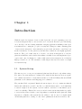
Chapter 1
Introduction
With the rapid development of sensor technologies and onboard computing power, autonomous navigation has become an active area of research. From Google’s self-driving
car to the iRobot home cleaning assistants, emerging applications utilizing technologies
from this field are coming into people’s everyday lives. Being two main consisting parts
of autonomous navigation, environmental perception and automatic control has been
studied extensively over the past few years and have resulted in some highly applicable
methods. The goal of this essay is to describe our efforts in integration of a mobile
platform in hardware and software that utilizes carefully chosen and implemented perception and control techniques to achieve fully autonomous navigation at a relatively
high speed and low cost. The remainder of this chapter introduces in detail of our high
level system setup.
1.1
System Set-up
The first step is to set up an experimental platform that allows for algorithm testing.
Two major test environment are evaluated here with the first that uses motion capture
for localization in an indoor environment and the second in the hallway that uses SLAM
(Simultaneous Localization and Mapping) for localization.
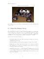
The purchased RC car (named Rustler shown in figure 1 above) contains mechanical
frames and built-in motors and controller box, which is much easier to work with than
a custom designed mobile system, but the built-in controller box has limited speed
control accessibility. This mobile car is a non-holonomic system that makes it possible
to test rear-wheel drived vehicle control algorithms on a much affordable platform. With
suspension on Rustler, this system has the ability to run in outdoor terrains which
extends this platform to testing of control and optimization methods from 2D to 3D.
1
Chapter1. Introduction
Figure 1.1: RC car test platform
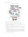
The following sections describes this experimental platform in terms of hardware and
software set-up.
1.2
Mobile Base Hardware Set-up
The experimental mobile platform contains a Traxxas Nitro Rustler car base with brushless back driving motor, and front servo motor for steering.The system runs on APC2
R AtomTM Processor Z550 (512K Cache, 2.00 GHz, 533 MHz FSB-)
computer with Intel
and DEll Vostro laptop with Intel(R) Core(TM) i7-3612QM CPU @ 2.10GHz.
Onboard sensors and actuators include:
• URG-04LX scanning laser range finder with 240 deg measuring area and 60 to
10000mm measurement range.
• ASUS Xtion PRO live is the vision sensor that used for slam or video stream.
• ATM203 Encoder is high accuracy axial modular encoder, which has a build in
SPI communication board. The encoder is mounted on the back wheel records the
absolute movement of the back wheel.
• 5GHz Wifi adaptor is used to seperate wifi signal. Communication between on
board computer and laptop is based on wifi connection. Currently, most wifi
signal is 2.4GHz,so this system used 5GHz wifi that can avoid interference from
most of the wif signals.
2
Chapter1. Introduction
Figure 1.2: System Flowchart
Laptop
User Interface
Graphic
parameter
Control
Command
Optimization Node
Laser
Joy Stick
state
Gmaping
Laser scan Control
command
Odometry
Kinect
Control Listener
Hokuyo Laser
Node
PWM
Wheel position
On-board Computer
&orientation
Car/Micro-controller
Encoder
Gyro
• Li-lon Polymer 7.4V 3 cell battery for computer power supply.
• 3900mAh 3 cell 11.1V G8 Pro battery for electronics power supply.
• Pololu 5V Stepdown Volt Reg converts the voltage output from battery to 5V
input voltage to micro-controller.
• Y-PWR, Hot Swap, Load Sharing Controller is ideal diode that two power sources
can be used together. This allows user to switch the power source without shutting
down the system.
• Arduino USB to Serial converter is used to connect micro-controller to onboard
controller. But power pin wasn’t connect to computer.Electronics and computer’s
power supply were separated to prevent restart of micro controller while the ROS
node start on computer or unstable random signal from power pin that leads to
restart of the micro controller board.
3
Chapter1. Introduction
• BeStar Acoustic Component (F-B-P3009EPB-01 LF) is sound actuator that beeps
when the battery runs low either on computer or electronics.
• Futaba R617FS 7-Channel 2.4GHz FASST Receiver receives control command
from Joystick.
• FUtaba T7C Joystick allows user manual remote control.
1.2.1
Sensor Calibration
In order for subsequent algorithm testings to accurately reflect their performance, careful
calibration of the onboard sensors is key. One of the first steps is to find a conversion
between the controller PWM signal to car speed and Steering angle. Motion capture
can measure the mobile robot position (x, y, θ) at 125 hz and is used here as the ground
truth. PWM signals from 1500 to 1800 with increments of 10 are fed as input commands
to the driving motor, while the steering servo motor remains neutral. Rustler will drive
at constant speed for around 1.5 m. Then,for each PWM input signal driving distance
1
can be estimated from motion captureD = (x2 + y 2 ) 2 , and the corresponding driving
speed can be estimated from the slope.
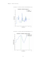
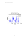
Figure 1.4: Motion Capture Distance
Figure 1.3: Input calibration
Estimation data at vehicle startup are ignored given that it takes time for the motor
to accelerate to certain speed. As can be seen from 1.3 and 1.4, each input PWM is
correlated to one spike. The conversion factor can be obtain from curve fitting the
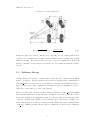
measured position data. Steering angle calibration utilizes very similar method (see
figure 1.5 for a simplified model of the vehicle). Commands are sent to the steering
motor with constant driving speed. The car will then drive in a circle and motion
capture will again log its position information. With know rear distance L, and driving
circle radius (δ), steering is calculated as equation 1.1. Due to the fact that both steering
wheels are controlled by the same servo, δ is consider same for both wheel.
4
Chapter1. Introduction
Figure 1.5: Steering Calibration
R=
q
cot δi + cot δo
a22 + l2 cot δ 2 cot δ =
2
(1.1)
Lastly, the wheel encoders are calibrated by comparing encoder reading with motion
capture pose. Command motor with constant PWM signal for driving, and neutral
signal for steering. The vehicle is then expected to drive at constant speed. It is then
trivial to establish a correspondence between the encoder readings and measured vehicle
velocity.
1.3
Software Set-up
Arduino Autopilot is a micro controller that reads in the sensor data and sent PWM
signal to actuators. The Rosserial library is used for Arduino-ROS communication.
Rosserial arduino sets up a rosnode on the Arduino board that can publish and subscribe
msg to/from rostopic. The computation on Arduino is kept at a minimum in order to
ensure the operational speed of the entire system.
Three nodes run on the onboard computer: CarControlListener, hokuyo node,and AMCL.
The CarControlListener node takes in sensor readings from the micro-controller and interpret the readings to meaningful data such as odometry, while at the same time takes
controller command and publish it to the hardware space such as motor PWM command. The Hokuyo node takes in readings from the Hokuyo laser sensor and publishes
/scan msg. AMCL (Adaptive Monte Carlo Localization) is a ROS based localization
5
Chapter1. Introduction
package that takes in odometry data and laser scan and outputs estimated robot location related to map.
Three nodes run on on-board computer: Gcop, Setwaypoint and Rviz. Gcop uses General Linear-Quadratic Regulator to compute local optimal path (discussed more in later
chapters). Setwaypoint takes in pre-designed global path and publish way points based
on robot current location. Rviz takes in whole frames and generate 3D graphic display
including the global map, robot frames and local optimal path.
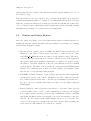
1.4
Control and Safety Feature
Since the vehicle is a high powered test platform that runs at relatively high speed,
making sure that the system can shut-down appropriately is a essential before starting
any automatic navigation testing.
1. The first part is joystick control. Normally, the Futaba T7C joystick is used for
AR.Drone control since it has a stable long range of round 50 meters. Standard APM RC APM2 library is used here for radio signal receiving. The microcontroller will only activate the motor and servo when it receives radio signal from
the joystick. Radio has 7 channels, 2 switch has to be turned on together to toggle
the vehicle to automatic driving mode,the rest of the channels are used for manual
joystick driving. The Microcontroller will sent continuous neutral PWM signals
(1500) to motor when the radio is turned on but not giving control signals to make
sure the motor won’t run under random signal.
2. NCURSES terminal UI (figure 1.6) is a simple user interface that displays the
current states (x, yθ) of the vehicle. All ROS nodes will be shut-down and the
motor will detached from the micro controller upon termination (currently set to
key ”Q”). ”D” is for command desired trajectory and ”I” for user input continuous
PWM signals.
3. Battery switch is connected directly from battery to electronics. Since previous
controls is either based on radio or wifi communication, a hard stop is designed
here to shut down the system power in case any communication issues occurs.This
switch will only shutdown the power supply to the electronics and micro-controller,
thus the onboard computer will remain running. However, no power line were
connect between the host computer and onboard computer, thus restarting the
electronics won’t affect ROS nodes on the host computer.
6
Chapter1. Introduction
Figure 1.6: User Interface
7
Chapter 2
Vehicle Odometry
Odometry is the use of motion sensor information for estimation of position over time.On
our mobile platform, odometry is obtained from a combination of encoder and gyro
sensor data. Here the position of the back wheels can be obtained from encoders and
vehicle’s orientation can obtained by processing gyro data. Although odometry will
diverge due to sensor drift, this divergence can be compensated by a measurement
update (details in the next chapter). But getting an accurate odometry estimate is an
essential first step for localization.
The vehicle’s states are usually presented as

x



 y 




 θ 


 v 


ω
(2.1)
where x and y are vehicle’s planar location and θ is the heading all in world coordinate.
vandω represents linear and rotational velocity. The pair of control inputs is the driving
velocity and steering angle
u
φ
8
!
(2.2)
Chapter 3. Vehicle Odometry
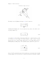
Figure 2.1: simple car model
The simple car model (illustrated in figure 2.1 ) can be written as

ẋ = u ∗ cos(θ)



 ẏ = u ∗ sin(θ) 


θ̇ = Lu tan(φ)
(2.3)
Assuming that sampling can be done at a fast rate, the position of the vehicle can be
reasonably estimated by

x = x + ẋδt



 y = y + ẏδt 


θ = θ + θ̇ ∗ δt
(2.4)
φ in equation 2.3 is the vehicle steering angle which can be obtain from the gyro. Dis
are the discrete encoder readings. In our first attempt to acquire accurate odometry
data, wheel speed u is obtained by finite differencing encoder readings, while front servo
PWM signals give turning angle φ. The dynamics update equations are given below
u = (D0 − D)/δt
u
θ0 = θ + tan φδt
L
x0 = x + u cos(θ)δt
(2.5)
y 0 = y + u sin(θ)δt
where [x0 , y 0 , θ0 ] represents the states at the next time step. A few issues arise from this
treatment.This model doesn’t take into account the fact that the steering angle command
9
Chapter 3. Vehicle Odometry
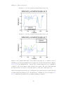
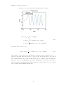
Figure 2.2: Odometry Calibration Result Without Gyro (X)
Figure 2.3: Odometry Calibration Result Without Gyro (Y)
signals does not transfer flawlessly to the actual steering angle due to a number of factor
including ground and mechanism friction, signal noise as well as inertial effects. Figures
2.2, 2.3, 2.4 below illustrates the odometry data obtained using the above formulation
compared to the ground truth obtained from motion capture. We can see that although
the data trend is correct most of the time (less so for X), there exists large error.
Our next attempt integrates the gyro readings into the system and θ is obtained directly
by numerically integrating the gyro measurement ω. Results are plotted in figures 2.5,
2.6, 2.7 which shows a much more promising tracking performance.
10
Chapter 3. Vehicle Odometry
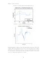
Figure 2.4: Odometry Calibration Result Without Gyro (θ)
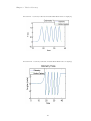
Figure 2.5: Odometry Calibration Result With Gyro (X)
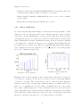
In the last attempt, we aimed for a smoother interpolation between gyro and encoder
readings. Therefore 10 integration steps are used between successive sensor readings.
Assume that for the small time interval t0 to t1 the gyro measurement stayed constant
at ω. It is desirable to find an expression that can estimate the vehicle location at time
t ∈ [t0 , t1 ]. Looking at the expression for x we have
11
Chapter 3. Vehicle Odometry
Figure 2.6: Odometry Calibration Result With Gyro (Y)
Figure 2.7: Odometry Calibration Result With Gyro (θ)
12
Chapter 3. Vehicle Odometry
Figure 2.8: Odometry Calibration Result With Curve Length
Z
t1
x(t) = x(t0 ) +
u cos(θ(t))dτ
t0
Z t1
u cos(θ(t0 ) + ω(τ − t0 ))dτ
= x(t0 ) +
(2.6)
t0
= x(t0 ) +
u
(sin(θ(t0 ) + ω(t − t0 ) − sin(θ(t0 ))
ω
the same can be done for y by
y(t0 ) = y(t0 ) +
u
(− cos(θ(t0 ) + ω(t − t0 ) + cos(θ(t0 ))
ω
(2.7)
Given such, as long as the sensor inputs stays constant, position estimates can be obtained for any time and can therefore be used to smooth out the trajectory between
sensor measurements. A problem for this method is gyro drifting. After 10 mins running, gyro error become significant. One feature is implemented as a temporary solution
where the user can use the provided UI or joystick to stop the vehicle for 5 sec, read in
sensor reading and reinitialize all the state.
13
Chapter 3. Vehicle Odometry
Figure 2.9: Odometry Calibration Result With With Curve Length (Y)
Figure 2.10: Odometry Calibration Result With With Curve Length(θ)
14
Chapter 3
Localization And Mapping
Mapping building is the first step of any fully autonomous driving operations. The
vehicle needs to understand the environment to be able to navigate. Simultaneous
Localization and Mapping also known as SLAM is widely used for such map building
applications.
3.1
Map Building
In this project, the ROS package slam gmapping is used to create an occupancy grid map.
The algorithm utilizes an improved version of the Rao-Blackwellized Particle Filter for
learning grid maps that results in the reduction of sampling size, thus effectively reducing
computation time.
For the general problem of mapping with particle filters, the goal is to estimate the joint
posteriro p(x1:t , m|z1:t , u1:t−1 ) for the map m and trajectory x1:t . The Rao-Blackwellized
particle filter simplifies the problem by making the factorization
p(x1:t , m | z1:t , u1:t−1 ) = p(m | x1:t , z1:t ) · p(x1:t | z1:t , u1:t−1 )
(3.1)
This factorization allows us to decouple the process of estimating the robot’s trajectory
and the map which greatly simplifys the problem. Given the above, the SLAM problem can be categorized into a four-step process of sampling - importance weighting resampling - map estimation. Because the length of trajectory increases over time, the
importance weighting step given by
15
Chapter3. Localization And Mapping
(i)
(i)
wt
=
p(x1:t | z1:t , u1:t−1 )
(i)
(3.2)
π(x1:t | z1:t , y1:t−1 )
can be very inefficient (π is the proposal distribution and p is the target distribution).
However if the proposal distribution can be restricted to fulfill
π(x1:t | z1:t , u1:t−1 ) = π(xt | x1:t−1 , z1−t , u1:t−1 · π(x1:t−1 | z1:t−1 , u1:t−2 )
(3.3)
then the weighting process can be massaged to a recursive form given by
wti =
ηp(zt | xi1:t , z1:t−1 )p(xit | xit−1 , ut−1 ) p(xi1:t−1 | z:t−1 , y1:t−2 )
·
π(xit | xi1:t−1 , z1:t , u1:t−1 )
π(xi1:t−1 | z1:t−1 , u1:t−2 )
p(zt | mit−1 , xit )p(xit | xit−1 , ut−1 )
i
∝
· wt−1
π(xt | xi1:t−1 , z1:t , u1:t−1 )
(3.4)
The contribution of gmaaping over conventional sampling based SLAM techniques with
grid maps is twofold. First, the proposal distribution is modified to consider the most
recent sensor measurement (if accurate) and sample only around that range. Second is
the introduction of an adaptive resampling technique based on the effective sample size
(Nef f ) measure to maintain a reasonable variety of samples. The proposal of the first
idea (modified proposal distribution) is motivated by the fact that if the measurement
model is highly concentrated (very precise) whereas the the proposal distribution is
highly distributed, it would take an enormous number of particles to produce a set
of weights that can accurately capture the target distribution. Assuming the target
distribution is unimodal, define an interval Li by
Li = {x | p(zt |it−1 , x) > }
(3.5)
and locally approximate the proposal distribution p(xt |mit−1 , xit−1 , zt , ut−1 ) around the
maximum of the likelihood function as a Gaussian. Then for each particle, a scanmatching algorithm can be used to provide the pose of maximum likelihood given the
map mit−1 and an initial guess, and in an interval (given by equation 3.5) around that
point a set of sampling points can be selected and their mean and covariance can be
calculated by
16
Chapter3. Localization And Mapping
K
uit
X
1
= i =
xj · p(zt | mit−1 , xj ) · p(xj | xit−1 , yt−1 )
η
(3.6)
j=1
Σit
K
1 X
p(zt | mit−1 , xl ) · p(xj | xit−1 , ut−1 )
= i·
η
j=i
(3.7)
·(xj − µit )(xj − µit )T
where
ηi =
K
X
p(zt | mit−1 , xj ) · p(xj | xit−1 , ut − 1)
(3.8)
j=1
and the new pose of particle i can be drawn from this improved proposal distribution
(which also proves to be the optimal proposal distribution). And using newly generated
particles the weights can be computed as
i
wti = wt−1
· p(zt | mit−1 , xit−1 , uit−1 )
Z
i
= wt−1 · p(zt | mit−1 , x0 ) · p(x0 | xit−1 , ut−1 )dx
i
' wt−1
·
K
X
(3.9)
i
p(zt | mit−1 , xj ) · p(xj | xit−1 , ut−1 ) = wt−1
· ηi
j=1
For the adaptive resampling process, the effective sample size given by
Nef f = PN
1
i=1 (w̃
i )2
(3.10)
is used to evaluate the performance of the current sample set in terms of representing
the target posterior. Nef f can be viewed as a measure of dispersion of the weights
(similar to covariance), if Nef f is too large, that means the estimated target distribution
is overly concentrated (or over-confident) which will result in the newly sampled particles
to lose diversity and ther efore could lead to localization failures. Therefore resampling
is only executed with Nef f is below a threshold thereby not only preserving the variety
of particles but also reduces computational cost.
However,even with gmapping, the speed of realtime map generation is limited (map
update speed is 1 hz). Therefore, for the purpose of testing our control algorithm, a map
of the experimental environment is built in advance using the slam gmapping package
17
Chapter3. Localization And Mapping
Figure 3.1: Kinect Framework
view_frames Result
Recorded at time: 1394135888.891
/optitrak
/camera_link
Broadcaster: /link2_broadcaster
Broadcaster: /camera_base_link1
Average rate: 50.031 Hz
Average rate: 10.164 Hz
Most recent transform: -0.017 sec old Most recent transform: -0.884 sec old
Buffer length: 4.897 sec
Buffer length: 4.821 sec
/map
/camera_rgb_frame
Broadcaster: /slam_gmapping
Average rate: 20.206 Hz
Most recent transform: 0.032 sec old
Buffer length: 4.850 sec
/odom
Broadcaster: /camera_base_link
Average rate: 10.174 Hz
Most recent transform: -0.673 sec old
Buffer length: 4.620 sec
/camera_depth_frame
Broadcaster: /camera_base_link3
Average rate: 10.173 Hz
Most recent transform: -0.851 sec old
Buffer length: 4.817 sec
/camera_rgb_optical_frame
Broadcaster: /camera_base_link2
Average rate: 20.120 Hz
Most recent transform: -0.881 sec old
Buffer length: 4.821 sec
/camera_depth_optical_frame
Broadcaster: /car_control_output
Average rate: 99.867 Hz
Most recent transform: -0.664 sec old
Buffer length: 4.997 sec
/base_link
and the AMCL(Adaptive MCL) package is then used for perception and provide the
vehicle’s position state estimates to the controller.
Two sensor are tested here for localization. The first is Kinect which is a low cost motion
sensor very popular for localization and mapping operations. The OpenNi ROS node
is well developed for the Kinect sensor with built-in sensor driver and image streaming
tools (package contained ROS nodes shown in figure 3.1). Here the Kinect point cloud
depth information is used to simulate laser information which makes implementation
of 2D SLAM methods possible. In addition, Kinect also has stereo vision and color
camera, that gives it the potential to obtain 3D map using RGDBSlam. Low sensor
detection range processing speed (10 fps) and resolution poses great limitation on the
usage of this sensor. Due to the above, a map(shown in figure 3.2) is generated by
using the slam gmapping package offline with the odometry and scan data logged from
teleoperating the vehicle.
The second is a Hokuyo laser range finder that gives a deg 240 detection angle range
and 10 hz of measurement frequency. This performance is well suited for the online
localization task that serves as the perception aspect of the controller
18
Chapter3. Localization And Mapping
Figure 3.2: Generate Occupancy Grid Map of Experimental Hallway
3.2
AMCL
The Adaptive Monte Carlo Localization (AMCL) is a localization package that implements the KLD-Sampling MCL Method for position tracking in 2D. The key to this
approach is to use a particle filter to adaptively vary the size of the sample set. The
result is a small sample size if the target distribution is tightly focused around a small
region and a larger sample size if it is distributed over a larger area (higher uncertainty), and therefore bound the approximation error. Such an error is measured by the
Kullback-Leibler distance that measures the difference between two probability distributions p and q given by
K(p, q) =
X
p(x)log
x
p(x)
q(x)
(3.11)
and hence the name KLD. Although the KL-distance is not a metric, it is widely adopted
as a standard measure for evaluating such differences. Refer to [4] for more details on the
approach. In addition, the AMCL package utilizes assistive algorithms from [3] such as
sample motion model odometry, beam range finder model, likelihood field range finder model,
Augmented MCL, and KLD Sampling MCL. The open source implementation of AMCL
is published as a ROS package that takes in the laser scan message, necessary transforms, an initial position and an occupancy grid map, and the outputs will be the
estimated robot pose, the estimated pose information of a set of particles maintained by
the algorithm as well as the tranforms necessary to map the results.
Error model is key to insure localization. Here, error model were obtained experimentally by compare the Odomety result with motion capture.Base on sensor rate 10 hz,error
model is compute as below:
19
Chapter3. Localization And Mapping
Figure 3.3: AMCL In Motion
alpha1: Specifies the expected noise in odometry’s rotation estimate from the rotational
component of the robot’s motion.
∆θOdom −∆θmotionCapture
∆θmotionCapture
= 0.08
alpha2: Specifies the expected noise in odometry’s rotation estimate from translational
component of the robot’s motion.
∆θOdom −∆θmotionCapture
∆dismotionCapture
= 0.2
alpha3: Specifies the expected noise in odometry’s translation estimate from the translational component of the robot’s motion.
∆disOdom −∆dismotionCapture
=0.8
∆dismotionCapture
alpha4: Specifies the expected noise in odometry’s translation estimate from the rotational component of the robot’s motion.
∆disOdom −∆dismotionCapture
=0.4
∆dismotionCapture
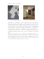
Because the experiment takes place in the hallway where no motion capture or other
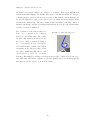
method can provide exact location information. Figure 3.3 provides a screenshot of
the system in operation. The vehicle in the back represents the current position (as
estimated by amcl) while the vehicle in front is the goal position. The white lines are
laser readings of the environment. And the green arrows are the particles performing
the localization task. The particles eventually converge to a small region. Figure below
shows the location and orientation result from AMCL method and compares it with a
picture of the physical surroundings. In figure 3.4, the red frame is the world frame,
blue is the vehicle frame, white areas represent unoccupied space whereas black and grey
areas are occupied by obstacles. Comparing it with figure 3.5 we can observe that the
the generated map can reasonably represent the physical world.
——————————————————————–
Although various localization algorithms are available, due to the system requirements
20
Chapter3. Localization And Mapping
Figure 3.4: AMCL Localization
Figure 3.5: Actual Robot location
and limitations, we found AMCL to be the most applicable package for this application.
Vehicle will mostly navigate in a planar region, thus a 2D map will be able to handle the
localization task. However, since AMCL doesn’t update the map, it is assumed for now
that navigation is done in a static environment. An implementation of the RGDB SLAM
is tested using Kinect but the image acquisition speed is limited to 2 hz which is not
enough for high speed online trajectory optimization, whereas the AMCL update speed
is based on laser data that is able to reach a 10 hz acquisition speed. Therefore based
o feasibility and system performance we have decided to use AMCL as our localization
method.
The major speed limitation is due to localization issue with high speed.Base on the
experiment data, Odometry accuracy doesn’t related to vehicle speed. However, the
error model might be the cause of inaccurate localization. Experiment were tested to
validate this assumption. In amcl, error model were setted as 500%,3.6 that the actual
error is larger than the experimental obtained error model.
21
Chapter3. Localization And Mapping
Figure 3.6: AMCL Odometry
22
Chapter 4
Trajectory Planning And
Tracking
This chapter serves as the theoretical core of this essay. In subsequent sections the underlying methods for optimal trajectory planning and tracking of the generated trajectory
are introduced along with a simulation of the optimal solver.
4.1
Dynamic Feedback Linearization
Dynamic Feedback linearization is a trajectory tracking approach that algebraically
transforms non-linear systems into linear systems, which proceeds by differentiating
the output y = h(x) enough time that the input appears linear and non-singular to
the output. By then the transformed linear system can be controlled using classical
methods. This is a easy-to-implement trajectory tracking scheme is used for various
validation tests at early stages of system integration.
4.1.1
Feedback Linearization for Simple Car Model
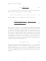
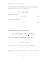
As a recap, the dynamics model for a simple car is given by

ẋ = u ∗ cos(θ)



 ẏ = u ∗ sin(θ) 


u
θ̇ = L tan(φ)
23
(4.1)
Chapter 4. Trajectory Planning And Tracking
where the two inputs are [u, φ] that represents the driving speed and steering angle. It is
obvious from the above model that input and output are related in a nonlinear fashion.
Differentiating the first two equations in 4.1 twice results in
!
ẍ = u̇s cos(θ) − u2s θ̇sin(θ)
(4.2)
ÿ = u̇s sin(θ) + u2s θ̇cos(θ)
Define the virtual inputs as
ẍ = v1
!
(4.3)
ÿ = v2
and the dynamic compensators as
ξ = u1
(4.4)
u2 = tan(uφ )
(4.5)
Also let
The resultant differentiated dynamics can be factorized as
" #
ẍ
"
# "
˙
ξcos(θ)
− L1 ξu2s sinθ
cos(θ)
=
=
1
2
˙
ÿ
sin(θ)
ξsin(θ)
+ L ξus cosθ
#" #
− L1 ξus sin(θ)
ξ˙
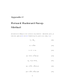
1
L ξus cos(θ)
u2
(4.6)
˙ u2 ] gives
solving the above system of two equations simultaneously for [ξ,
ξ˙ = v1 cos θ + v2 sin θ
u2 = ((v2 cos θ − v1 sin θ)/ξ 2
(4.7)
let ~v = [v1 , v2 ]T and ~y = [x, y]T , since ~v = ~y¨, a stable control law is given by
~v = ~y¨d − kp (~y − ~yd ) − kd (~y˙ − ~y˙ d )
(4.8)
To see that the above control is stable, equation 4.8 can be rewritten in a state space
form as
24
Chapter 4. Trajectory Planning And Tracking
Figure 4.1: Feedback Linearization controller simulation result
#
#"
# "
"
~y − ~yd
0
I
~y˙ − ~y˙ d
=
−kp −kd ~y˙ − ~y˙ d
~y¨ − ~y¨d
(4.9)
for positive definite kp and kd , system 4.9 is globally asymptotically stable. And resulting
virtual inputs can be mapped to physical inputs using equation 4.7
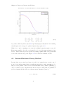
With above control, a simulation is conducted in Matlab using the simple car model.
From start point X0 = [0, 5, 0] to goal point Xf = [5, 2.5, 0], the start and final velocity
are zero. The desired trajectory is generated by fitting a quintic (fifth order) polynomial
between the start and end points. Figure 4.1 below shows the simulation result.
4.2
Forward-Backward Sweep Method
Because what we are aimed at solving for is the local optimal trajectory and control,
it can be reasonably assumed that for small time intervals no path constraint is to be
imposed on the planner. Therefore the Forward-Backward Sweep Method (FBSM) [] []
can be a relatively easy to implement and effective way for solving such an optimization
problem. Assume that the discrete nonlinear system dynamics is given by
xi+1 = f i(xi , ui ),
25
(4.10)
Chapter 4. Trajectory Planning And Tracking
and here we use a linear quadratic cost function of the form
J0 = LN (xN ) +
N
−1
X
Li (xi , ui )
i=0
N
−1
X
1 T
1 T
= x (N )Pf x(N ) +
(x Qxi + uTi Rui )
2
2 i
(4.11)
i=0
and define the cost-to-go to be the above cost from current to the end (Ji = LN (xN ) +
NP
−1
Li (xi , ui )). The goal is to locally optimize the Hamiltonian-Jacobi-Bellman (HJB)
i
value function at each step defined by
Vi (x) = min Ji (x, ui:N −1 )
(4.12)
ui:N −1
and the above value at time i is written in a recursive form by
Vi (x) = min Qi (x, u) = min{Li (x, u) + Vi+1 (fi (x, u))}
u
u
(4.13)
where Q is the unoptimized value function. To minimize Q at step i, the perturbation
around i is defined as
∆Qi (δxi , δui ) = Li (xi +δxi , ui +δui )−Li (xi , ui )+Vi+1 (f (xi +δxi , ui +δui ))−Vi+1 (xi , ui )
(4.14)
Expanding the above equation to second order results in

∆Qi ≈
1
T 
∇x QTi
0
∇u QTi

1

 
 
1
δxi  ∇x Qi ∇2 Qi ∇xu Qi  δxi 
x
 



2
2
δui
∇u Qi ∇ux Qi ∇u Qi
δui
(4.15)
Given the principle of optimality, the choice of δui should minimize ∆Q, in other words
∂∆Q
=0
∂δui
(4.16)
δu?i = Ki · δxi + αi ki
(4.17)
which gives the optimal δu as
26
Chapter 4. Trajectory Planning And Tracking
Figure 4.2: Feedback Linearization controller simulation result
where
Ki = −∇2u Q−1
i ∇ux Qi
(4.18)
ki = −∇2u Q−1
i ∇u Qi
(4.19)
and α is the step size chosen such that the controls result in a sufficient decrease in the
value function.
With the above conclusions, a forward-backward process can be implemented to calculate
the controls that yield locally optimal trajectory according to the designed cost function.
The algorithm first steps backwards in time and recursively find Ki and ki as defined
in equations 4.18 and 4.19. Incorporating these values with the system dynamics, the
controls are then updated forward in time. This forward backward process is repeated
until convergence of the cost function. Details on the step-through of the algorithm is
provided in Appendix C. This method is simulated in ROS with visualization results
shown in figure 4.2. The vehicle in the back and front illustrates current and goal
position respectively, and the blueline denotes the computed optimal trajectory.
27
Chapter 5
Results And Discussion
5.1
Experiment Description and Results
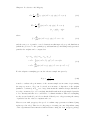
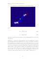
This chapter shows some of experimental results along with discussions of their significance. Given the floor map shown in Chapter 3, the vehicle is to autonomously navigate
itself through the area while avoiding obstacles.
The path that the vehicle takes should also be locally optimal according to the calculation
in the previous chapter. The relationship between the vehicle and world frame as well
as the definition of frames within the vehicle is illustrated in Appendix B. It is necessary
to not that since the brushless motor that drives the vehicle has a large minimal speed,
while the AMCL method cannot provide an accurate estimate if robot runs at high speed
Figure 5.1: Computed vs. Actual Trajectory in Controller Testing
28
Chapter 5. Results and Discussion
Figure 5.2: Video Screenshot
(state update is not able to catch up with actual position change). Therefore parameter
optimization is limited on control of velocity input signal by setting very small R in
the cost function given by 4.11. Figure 5.1 shows the FBSM computed optimal/desire
trajectory compared to the actual executed trajectory record by motion capture in an
in-lab calibration test. We can see that the overall trend is correct and the discrepency
is within a relatively small range (max around 20cm). The short distance traveled is
due to limited lab space.
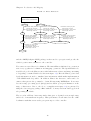
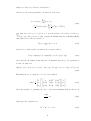
Global trajectory is pre-selected as the red dots showing in the figure 5.2. The goal
speed was assumed constant. Blue line in the same figure shows local optimal trajectory
computed using the Direct Sweep Method. The algorithm uses the vehicle’s current
location as the initial position and last step speed as initial speed. Final position is the
5th closet point in global trajectory in the direction of the current heading. The result
demonstrates that mobile robot was able to track the trajectory for 10 loops at 1 m/s.
The video compares real world vehicle view (recorded using the onboard Kinect) with the
Rviz visual environment (with the graphics generated by sensor and command messages).
The Video in the attachment shows the entire process of loop trajectory optimization
and tracking. Note that the vehicle is manual stopped on the end off the hallway due
the internet connection lose.
5.2
Future Work
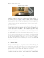
Although odometry is not suppose to give perfectly accurate localization. But improving
odometry result over time will certainly result in a better localization performance. With
a better odometry model, the number of particles used for localization can be reduced
which gives a faster computational time and a higher rate of state update.
The magnetometer is there to provide a constant reference (magnetic north) which
compensates for the drift of the gyroscope. Therefore fusing the gyro and magnetometer
29
Chapter 5. Results and Discussion
information can greatly enhance the accuracy of odometry. There is an IMU(Inertial
measurement unit) built into the Arduino Auto pilot board, which in addition to the gyro
contains a magnetometer as well as an accelerometer. But with the current hardware set
up, several magnets are used for the battery case cap which affects the magnetometer
measurement dramatically. Therefore future design can include removing sources of
magnetic interference and incorporating additional sensors for noise removal and higher
accuracy orientation estimation.
The orientation of the vehicle ranges for
Figure 5.3: issue with trajectory
from −π to π and the solver computes
trajectory only in this range. The resulting issue that arises is shown in the figure below.
With a starting heading of
θ0 = −3rad and a goal of θf = 3.1rad, the
solver will calculate optimal control input
as turning in the direction that crosses
zero (since mathematically there’s only
one direction to go from -3 to 3.1 on the
real line). But simply by adding a 2π wrap-around doesn’t completely solve the problem. This issue renders the optimizer to give suboptimal trajectories in situations like
this and is worth the effort to look at in the future.
30
Chapter 6
Conclusion
This essay aims at introducing a complete system integration process for high speed/low
cost autonomous navigation testbeds from hardware to software and finally choice of
perception and control schemes. Limitations on both the hardware processing power
and software computational time restricts how high a speed the vehicle can accurately
and reliably navigate itself. The proposed system uses a collection of standard off-theshelf mechanical and electrical components. At the time of experimentation, the onboard
computer used is not powerful enough to handle the localization and control algorithms,
so this part is done on a host laptop and onboard computer handles only collection of
sensor data and execution of command given by the host computer. Communication is
established via the Wifi network and a large restriction on the overall performance is
imposed by communication speed and reliability (drop of packets, lost connection, etc).
Therefore it is worthwhile to try and migrate all compution onto the vehicle which makes
the system more closely meet the standard of full autonomy. The choice of gmapping
as our SLAM method due to its ability to draw particles in a more accurate way and
thus dramatically reduces the required number of samples and unncecessary resampling
actions. For our online localization algorithm, AMCL is chosen for its simplicity in
terms of implementation as well as adequate perform for our purposes. The ForwardBackward Sweep Method is used as our locally trajectory planning and tracking scheme
given its effectiveness in generating locally optimal trajectories while also providing a
feedback control law. Overall the proposed system has achieved stable and continuous
autonomous navigation circumventing the close loop hallway as described in chapter 3
with an average speed of 1 m/s. Much room exists for discussion and improvement,
but this essay serves as a detailed guidance in implementing related systems as well as
considerations necessary in the choice of navigation schemes.
31
Appendix A
Experiment procedure
1. Set-up system hardware and joystick control
2. Feedback linearization control using motion capture to localize
3. sweep method and dynamic programming control using motion capture localize
4. Kinetic visual slam using motion capture fake odometry
5. Slam using laser sensor and fake odometry
6. slam gmapping with kinematic model odometry
7. Integration of Slam and differential dynamic programming
32
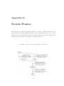
Appendix B
System Frames
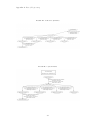
The following are detailed diagrams showing the correlation of different frames used by
the system, the node that publishes them (broadcaster) as well as their rate of broadcast.
This information is important in terms of verification that the system is software-wise
integrated properly and is very useful for debugging purposes.
Figure B.1: Position of The Vehicle Relative to The World
33
Appendix A. List of Project step
Figure B.2: Vehicle Body Frames
Figure B.3: system frames
34
Appendix C
Forward Backward Sweep
Method
As mentioned in Chapter 4, the backwards sweep finds the coefficients Ki and ki as
defined in equations 4.18 and 4.19. Detailed steps are given by (according to [5])
Vx = ∇LN
(C.1)
Vxx = ∇2x LN
(C.2)
k =N −1→0
(C.3)
Qx = ∇x Li + ATi (Vxx )Ai
(C.4)
Qu = ∇u L + B T Vx
(C.5)
Qxx = ∇2x Li + ATi (Vxx )Ai
(C.6)
Qu u = ∇2u Li + BiT (Vxx )Bi
(C.7)
35
Appendix C. List of Project step
Qux = ∇u ∇x Li + BiT (Vxx )Ai
(C.8)
ki = −Q−1
uu Qu
(C.9)
Ki = −Q−1
uu Qux
(C.10)
Vx = Qx + KtT Qu
(C.11)
Vxx = Qxx + DT Qux
(C.12)
While the forward sweep updates the controls by
δx0 = 0,
(C.13)
V0 0 = 0
(C.14)
k =0→N −1
(C.15)
u0i = ui + αki + Ki δxi
(C.16)
x0i+1 = fi (x0i , u0i )
(C.17)
δxi+1 = x0i+1 − xi+1
(C.18)
Vo0 = Vo0 + Li (Xi0 , u0i )
(C.19)
Vo0 = V00 + LN (x0N )
(C.20)
36
Bibliography
[1] G. Grisetti, C. Stachniss, and W.Burgard. Improved Techniques for Grid Mapping
With Rao-Blackwellized Particle Filters. IEEE Transactions on Robotics, 2007.
[2] G. Grisetti, C.Stachniss, and W.Burgard. Improving Grid-based SLAM with RaoBlackwellized Particle Filters by Adaptive Proposals and Selective Resampling. In
ICRA Robots and Automation, 2005.
[3] S. Thrun, W. Burgard, and D. Fox. Probabilistic Robotics. The MIT Press, 2006.
[4] Dieter. Fox. Adapting the Sample Size in Particle Filters Through KLD-Sampling.
Internation Journal of Robotics Research, 22, 2003.
[5] M. Kobilarov. EN530.603 Applied Optimal Control EN530.603 Applied Optimal
Control. Lecture 9: Numerical Methods for Deterministic Optimal Control, October
2013.
37
Biographical Statement
Ying Xu was born July 5th,1989 in Wuhan, China. She completed her undergraduate
studies at Iowa State University in Mechanical Engineering. After that she started her
graduate work at Johns Hopkins University, Baltimore obtained he MSE in Mechanical
Engineering under the Robotics Track in 2014.
38