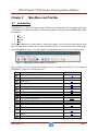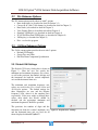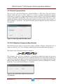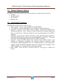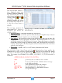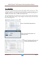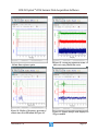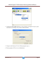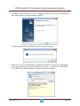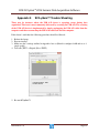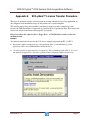
1
SC3-μSeis™
2014
User’s Reference Manual
Version 14.1.0 – February 2014
.
BCE SC3-µSeis™ 2014 Seismic Data Acquisition Software
BCE’s mission is to provide our clients around the world with state-of-the-art seismic data
acquisition and analysis systems, which allow for better and faster diagnostics of the subsurface.
The company provides state-of-the-art hardware and software solutions for a wide variety of
seismic engineering applications. If necessary, we will customize our products to suit the
requirements of our clients even better.
BCE's products and services consist of
• Seismic Data Acquisition and Signal Conditioning Hardware
• Seismic Data Processing Software
• Applied Seismology Consulting Services
• Seismic Data Processing
• Professional Seminars
By publishing this manual we will hopefully provide a better understanding of downhole seismic
testing and the role it can play in geotechnical investigations.
Baziw Consulting Engineers Ltd
3943 West 32nd Avenue Vancouver B.C. Canada V6S 1Z4
url: www.bcengineers.com
email: [email protected]
© 1998 - 2014 Baziw Consulting Engineers Ltd.. All rights reserved. The content on this work is
protected by the copyrights of Baziw Consulting Engineers Ltd.. No part of this document may
be reproduced, stored in a retrieval system, or transmitted in any form or by any means,
electronic, mechanical, photocopying, or otherwise without the prior written permission of
Baziw Consulting Engineers Ltd. Although every precaution has been taken in the preparation
of this manual, we assume no responsibility for any errors or omissions, nor do we assume
liability for damages resulting from the use of the information contained in this manual
Revision 14.1.0
Page i
BCE SC3-µSeis™ 2014 Seismic Data Acquisition Software
Table of Contents
Chapter 1
Introduction ..............................................................................................................1
1.1 What is SC3-µSeis™? .......................................................................................................1
1.2 Organization of users manual ............................................................................................2
Chapter 2
Main Menu and Tool Bar .........................................................................................3
2.1 Introduction........................................................................................................................3
2.2 File Submenu Options .......................................................................................................4
2.3 Utilities Submenu Options .................................................................................................4
2.3.1 Default GUI Settings .....................................................................................................4
2.3.2 Sensor Type and Units ...................................................................................................5
2.3.3 Full Waveform Component Specification .....................................................................5
2.4 Window Submenu Options ................................................................................................6
2.5 Help Submenu Options ......................................................................................................6
Chapter 3
Seismic Data Acquisition .........................................................................................7
3.1 Data File Specification and A/D Parameters .....................................................................7
3.2 Trigger Parameters ...........................................................................................................10
3.2.1 Trigger Parameters.......................................................................................................10
3.2.2 SEED™ Algorithm Event Detection Parameters ....................................................... 11
3.2.3 Pretrigger Parameters ..................................................................................................13
3.3 Begin Acquisition and Stop Acquisition Tool Bar ..........................................................13
3.4 Convert to SC3-Rav™ File Format .................................................................................14
3.5 Data Stack ........................................................................................................................16
Chapter 4
View Seismic Data .................................................................................................17
4.1 View Seismic Data ...........................................................................................................17
4.2 Standard VSP Display......................................................................................................20
4.3 X-Y-Z-Full Waveform VSP Display ................................................................................22
4.4 3D Display .......................................................................................................................25
Chapter 5
Chart Formatting, Exporting, and Printing.............................................................28
Chapter 6
References ..............................................................................................................29
Appendix 1 E. Baziw and G. Verbeek, “Passive (Micro-) Seismic Event Detection by
Identifying Embedded “event” Anomalies within Statistically Describable Background Noise”,
Pure Appl. Geophys., vol. 169, issue 12, pp. 2107-2126, Dec. 2012............................................30
Appendix 2 E. Baziw, "Real Time Seismic Signal Enhancement Utilizing a Hybrid Rao
Blackwellised Particle Filter and Hidden Markov Model Filter", IEEE Geosci. Remote Sensing
Letters, vol. 2, no. 4, pp. 418- 422, Oct. 2005. ..............................................................................31
Appendix 3 BCE technical note entitled “Passive (Micro-) Seismic Event Detection by
identifying, quantifying and extracting frequency anomalies within statistically describable
background noise”. ........................................................................................................................32
Appendix 4 SC3-µSeis™ Installation Procedure .......................................................................33
Appendix 5 SC3-µSeis™ Trouble Shooting ..............................................................................36
Appendix 6 SC3-µSeis™ License Transfer Procedure ..............................................................37
Revision 14.1.0
Page ii
BCE SC3-µSeis™ 2014 Seismic Data Acquisition Software
List of Figures
Figure 1: Main Menu and Tool Bar in SC3-µSeis™ ...................................................................... 3
Figure 2: Default GUI Settings ....................................................................................................... 4
Figure 3: Sensor Type and Units dialog boxes ............................................................................... 5
Figure 4: Full Waveform Component Specification User Interface ............................................... 5
Figure 5: File Menu ........................................................................................................................ 7
Figure 6: Directory Selection Dialog Box ...................................................................................... 7
Figure 7: Trigger Parameters Input Screen ................................................................................... 10
Figure 8: Finite difference source wave with superimposed 140 Hz sinusoid and exponential
decay with rate 0.8/ms ...................................................................................................................11
Figure 9: Low pass filtered (900 Hz) sensor data (green trace), STA/LTA of smoothed AMT (red
trace), and Smoothed AMT (blue trace)........................................................................................ 12
Figure 10: SC3-µSeis™ tool bar ................................................................................................... 14
Figure 11: Convert to SC3-Rav™ File Format user interface ...................................................... 14
Figure 12: File→ Convert to SC3-Rav™ File Format file input dialog box ................................ 15
Figure 13: Data Stack file input dialog box .................................................................................. 16
Figure 14: Specifying the format to save stacked time series ....................................................... 16
Figure 15: Specifying the directory and file name of the stacked time series .............................. 16
Figure 16: Main graphical interface in View Seismic Data software option ................................ 17
Figure 17: Filter Parameter Specification Window ...................................................................... 17
Figure 18: Filtered seismic trace in View Seismic Data software option ..................................... 18
Figure 19: Overlaying unfiltered seismic time series onto filtered time series ............................ 18
Figure 20: Display of frequency spectrum of seismic time series illustrated in Figure 18 .......... 18
Figure 21: Seismic data file with Display Pre-Trigger enabled .................................................... 18
Figure 22: Seismic data before time shift ..................................................................................... 19
Figure 23: Seismic data after time shift of -3.36 ms ..................................................................... 19
Figure 24: Depth Profile dialog box ............................................................................................. 20
Figure 25: Depth Profile graphical interface box ......................................................................... 20
Figure 26: Filtered (30 to 100 Hz bandpass) Standard VSP Display seismic trace profile
illustrating color coded reverse polarized waves .......................................................................... 21
Figure 25: Display of the PPA Values for the X-Component Time Series Data ........................... 22
Figure 26: Example of X-Y-Z-Full Waveform VSP Display Output where the X-component, Ycomponent, Z-component, and Full Waveform Seismic Time Series Data is Displayed ............. 23
Figure 27: Seismic Time Series Data Shown in Figure 28 with the Globally Normalization
Option Enabled ............................................................................................................................. 23
Figure 28: Illustration of PPA Values for Captured Triaxial Data. In addition, the interval velocity
between depths 1.0 m and 2.0 m is shown .................................................................................... 24
Figure 29: Typical 3D Display (data unfiltered) ........................................................................... 25
Figure 30: 2D display of the FFT results of the filtered data shown in Figure 32 ........................ 26
Figure 31: Typical 3D Display (same data as in Figure 31, but now filtered and chart copied to
clipboard as described below)....................................................................................................... 26
Figure 35: Chart Editing Dialog Box ............................................................................................ 28
Figure 36: Chart Printing Dialog Box ........................................................................................... 28
Revision 14.1.0
Page iii
BCE SC3-µSeis™ 2014 Seismic Data Acquisition Software
Chapter 1
1.1
Introduction
What is SC3-µSeis™?
SC3-µSeis™ is a Windows® program that facilitates the autonomous data acquisition of triaxial
Seismic Cone (SC) time series data. SC3-µSeis™ utilizes passive (micro-) seismic monitoring
technology where a dedicated trigger channel remotely discerns whether an “event” or “trigger”
has occurred. When an “event”or a“trigger” is detected the SCPT seismic data is stored to file at
the user specified sampling rate and sample time.
SC3-µSeis™ allows for a Contact or Sensor trigger. The Sensor trigger is based on BCE’s socalled SEED™ (Signal Enhancement and Event Detection) algorithm, which uses real time
Bayesian Recursive Estimation (BRE) digital filtering techniques to analyze in real-time the raw
trigger data.
SC3-µSeis™ includes the following features:
Configurable for either geophones or accelerometers.
Configurable for either Contact or Sensor trigger.
Implementation of the SEED™ algorithm.
Short term average / long term average (STA/LTA) event detection.
Automatic data gain setting.
Suitable for P-Wave and S-wave.
Maximized data sampling rate.
Ability to save trigger channel and pre-trigger data to file.
Functionality to convert acquired seismic data into the SC3-RAV™ data format.
Option for post data stacking.
Bandpass, high pass, low pass, and notch digital filters.
Automatic full waveform SH-wave interval velocity estimates.
Displays of peak particle accelerations, velocities, and displacements.
VSPs with trend line estimation.
3D Displays of VSP Profiles.
Revision 14.1.0
Page 1
BCE SC3-µSeis™ 2014 Seismic Data Acquisition Software
1.2
Organization of users manual
The purpose of this manual is to instruct users of SC3-µSeis™ in the use of the product by
explaining its structure, taking the user step by step through the program menus, and specifying
the use of interactive graphics and I/O routines.
In addition, the manual contains the following items:
•
•
•
•
•
Appendix 1 provides a copy of the paper entitled “Passive (Micro-) Seismic Event
Detection by Identifying Embedded “event” Anomalies within Statistically Describable
Background Noise”. This paper outlines the most recent formulation of the SEED™
algorithm.
Appendix 2 provides a copy of the paper entitled “Real-time seismic signal enhancement
utilizing a hybrid Rao–Blackwellized particle filter and hidden Markov model filter.”
This paper outlines the initial mathematical details behind the SEED™ algorithm.
Appendix 3 provides a copy of the BCE technical note entitled “Passive (Micro-)Seismic
event detection by identifying, quantifying and extracting frequency anomalies within
statistically describable background noise”. This technical note concisely outlines the
SEED™ algorithm and provides examples of the advantages of the SEED™ algorithm
over standard frequency filtering techniques.
Appendix 4 provides the user with a detailed installation procedure for this software.
Appendix 5 offers the user some SC3-µSeis™ trouble shooting tips.
WARNINGS:
•
•
This program requires a 64 bit Windows operating system
To ensure that the program will function properly it is important
that it is installed correctly as outlined in Appendix 4.
Revision 14.1.0
Page 2
BCE SC3-µSeis™ 2014 Seismic Data Acquisition Software
Chapter 2
2.1
Main Menu and Tool Bar
Introduction
SC3-µSeis™ is a Windows® program that facilitates the autonomous data acquisition of triaxial
seismic cone (SC) time series data. As illustrated in Figure 1 the main menu of SC3-µSeis™ has
four options:
• File
• Utilities
• Window.
• Help.
The desired submenu is chosen either by moving the mouse over the desired option and pressing
the left hand mouse button, by pressing function <F10> on the keyboard and selecting the
desired highlighted option, or by pressing the corresponding menu item letter on the keyboard.
Figure 1: Main Menu and Tool Bar in SC3-µSeis™
The program can also be operated by clicking on icons. As illustrated in Figure 1 the toolbar of
SC3-µSeis™ consists of 15 different icons:
Description
Icon
Data Acquisition
Convert to SC3-RAV™ File Format
Data Stack
View Seismic Data
Standard VSP Display
X-Y-Z Full Waveform Display
3D Display
Default GUI Settings
Sensor Type and Units
Full Waveform Component Specification
Manual Section
3
3.4
3.5
4.1
4.2
4.3
4.4
2.3.1
2.3.2
2.3.3
Cascade
Tile Horizontally
Tile Vertically
2.4
2.4
2.4
About
Open User’s Manual
2.5
2.5
Revision 14.1.0
Page 3
BCE SC3-µSeis™ 2014 Seismic Data Acquisition Software
2.2
File Submenu Options
The File menu option provides the user with 7 options:
• Data Acquisition (as described in detail in Section 3.1)
• Convert to SC3-Rav™ file format (as described in detail in Chapter 3)
• Data Stack (as described in detail in Chapter 3)
• View Seismic Data (as described in detail in Chapter 4)
• Standard VSP Display (as described in detail in Chapter 4)
• X-Y-Z Full Waveform VSP Display (as described in Chapter 4)
• 3D Display (as described in Chapter 4)
• Exit – to close the program
2.3
Utilities Submenu Options
The Utilities menu option provides the user with 3 options
• Default GUI Settings
• Sensor Type and Units
• Full Waveform Component Specification
2.3.1 Default GUI Settings
The Default GUI Settings dialog box is shown in
Figure 2.
Here the user can specify the
minimum and maximum frequency axis values,
as well as the precision, the number of digits and
the increment for both the vertical amplitude
axis and the horizontal time axis.
The minimum and maximum frequency axis
values are used for the View Seismic Data and
3D Display options. The default settings for
these frequencies are zero and the Nyquist
frequency (1/2∆, where ∆ is the sampling rate)
respectively. If the user wishes to change these
values, then check box Enable should be
checked and the appropriate minimum and
maximum frequencies should be specified.
The precision, the number of digits and the
increment for both the vertical amplitude axis Figure 2: Default GUI Settings
and the horizontal time axis are used for all
charts displayed within SC3-µSeis™.
Revision 14.1.0
Page 4
BCE SC3-µSeis™ 2014 Seismic Data Acquisition Software
2.3.2 Sensor Type and Units
The Sensor Type and Units dialog box is shown in Figure 3. The Sensor Type Specification
interface allows the user to specify whether Accelerometers (output proportional to particle
acceleration) or Geophones (output proportional to particle velocity) are used for the downhole
seismic testing (DST) investigation. The Unit Specification interface allows the user to select
whether the particle velocities and accelerations recorded are given in units of m/s and m/s2 or
mm/s and mm/s2, respectively. This directly depends upon the amplitude units the seismic data
was stored in.
Figure 3: Sensor Type and Units dialog boxes
2.3.3 Full Waveform Component Specification
The Full Waveform Component Specification option as shown in Figure 4 allows the user to
disable or enable X, Y or Z axis recordings within the full waveform calculation and analysis.
The absolute value of the full waveform is defined as
The constants A, B, or C are set to either 0 or 1 depending on whether the related axis has been
enabled or disabled. This option covers the situation where there have been faulty recordings on
a specific axis and the user does not want to incorporate this time series within the analysis of the
full waveform within the VSP displays. It should be noted that whenever SC3-µSeis™ is started,
the X Axis, Y Axis and Z Axis parameters are enabled.
Figure 4: Full Waveform Component Specification
User Interface
Revision 14.1.0
Page 5
BCE SC3-µSeis™ 2014 Seismic Data Acquisition Software
2.4
Window Submenu Options
The Window menu option provides the user with 4 options to arrange the open window(s):
• Cascade
• Tile Horizontally
• Tile Vertically
• Minimize All
2.5
Help Submenu Options
The Help option provides the user with 3 options:
• About - provides software version information on SC3-µSeis™.
• User’s Manual - opens the SC3-µSeis™ user’s manual in a default pdf browser.
• Appendix 1 opens the paper entitled “Passive (Micro-) Seismic Event Detection by
Identifying Embedded “event” Anomalies within Statistically Describable Background
Noise” in a pdf browser. This paper outlines the most recent formulation of the SEED™
algorithm.
• Appendix 2 opens the paper entitled “Real-time seismic signal enhancement utilizing a
hybrid Rao–Blackwellized particle filter and hidden Markov model filter.” This paper
outlines the initial mathematical details behind the SEED™ algorithm.
• Appendix 3 opens the BCE technical note entitled “Passive (Micro-)Seismic event
detection by identifying, quantifying and extracting frequency anomalies within
statistically describable background noise” in a default pdf browser. This technical note
concisely outlines the SEED™ algorithm and provides examples of the advantages of the
SEED™ algorithm over standard frequency filtering techniques.
• Link to BCE - opens the Baziw Consulting Engineers’ web page in a default web
browser.
Revision 14.1.0
Page 6
BCE SC3-µSeis™ 2014 Seismic Data Acquisition Software
Chapter 3
Seismic Data Acquisition
The File→Data Acquisition menu
option is used to carry out
autonomous data acquisition and
allows the user to communicate with
the BCE signal conditioning board
and the analog/digital (A/D)
conversion board. As shown in
Figure 5, this menu has two tabs for
data input:
• Data File Specification and
A/D Parameters.
• Trigger Parameters.
Once the data has been entered, the
tool bar at the top of the screen is
used to control the actual data
acquisition.
Figure 5: File Menu
3.1
Data File Specification and A/D Parameters
The Data File Specification and A/D Parameter tab is illustrated in Figure 5 and the input
parameters required on this tab are as follows:
• Site Name – the user specified Site Name is utilized
within SC3-µSeis™’s automatic seismic data file
naming and saving process. The default Site Name is
uSEIS
• Data Directory - the default data file storage
directory is selected by pressing the directory list
icon . Figure 6 illustrates the dialog box which
appears when this icon is selected. The user browses
the available drives and directories and selects the
one most appropriate for seismic data file storage.
• Save Data As - the user has the option to store
seismic data in either ASCII or binary file formats by
selecting the appropriate radio button. The default
filenames are *.aci for ASCII file formats and *.bin
for Binary file formats. Binary file formats are Figure 6: Directory Selection
desirable because they typically require less memory Dialog Box
storage, while ASCII data files can easily be read into
other programs. The default format is Binary.
• Source Wave Type - S-wave (S) or P-wave (P) - dominant source wave type under
analysis. The default wave type is S-wave.
Revision 14.1.0
Page 7
BCE SC3-µSeis™ 2014 Seismic Data Acquisition Software
A typical file name for a seismic file saved is outlined and defined as follows:
uSEISS_28_01_2014 15_15_25_152.bin
uSEIS
S
28_01_2014
15_15_25_152
.bin
specified by the user in the Site Name edit box
S-wave (S) or P-wave (P) - dominant source wave type
day data acquired (i.e., day_month_year)
time data acquired (i.e., hour-minute-sec-msec)
user specified data type
If option Save Trigger Channel to File option is enabled (see Section 3.2) the associated saved
trigger file includes TRIG prior to the day information (e.g., uSEISS_TRIG28_01_2014
15_15_25_152.bin).
Apart from the Data File Specification input the user also has to enter the following:
• Radial Offset - radial offset (m) of the source from the penetration cone.
• Source Depth - depth (m) of the source into the ground.
• Data Gain - the data gain corresponds to the amplitude gain on the recorded data, and
can be set from 0 to 84 dB in increments of 6 dB. The default Data Gain is 30 KHz.
• Sampling Rate - the sampling rate is specified in KHz and it ranges in value between 1
and 50 KHz. The default Sampling Rate is 20 KHz.
Once the user has specified the Sampling Rate, the program will determine the Actual
Sampling Rate, which is a multiple of the specified Sampling Rate, to take optimal
advantage of the fact that a digital trigger is used.
Listed below are the Actual Sampling Rates for each of specified Sampling Rate for both
the Contact trigger and the Sensor trigger (see Section 3.2):
Sampling Rate (KHz)
2
3
4
5
6
7
8
9
10 20 30 40 50
Specified 1
Actual
contact 125 120 120 120 125 120 140 160 180 120 120 120 120 150
sensor 20 20 18 20 20 18 21 24 18
20 30 40 50
From the table above it is clear that there is a distinct difference in actual sampling rates
depending on the trigger type. This is due to the computational requirements of the
SEED™ algorithm used with a sensor trigger. This algorithm must complete filtering and
event detection within ∆×ring buffer size prior to extracting the next set of data from the
ring buffer. This means that the maximum allowable processing time for a 8192 point
ring buffer and a sampling rate of 20 KHz is 410 ms. Performance testing of the SEED™
algorithm has shown that it requires approximately 140 ms to process 8192 data points
with a sampling rate of 20 KHz, or approximately 1/3 of the maximum allowable
processing time. The computer system utilized for this test was a Dell Latitude E6520
laptop with a quad-core 2.40 GHz CPU.
Revision 14.1.0
Page 8
BCE SC3-µSeis™ 2014 Seismic Data Acquisition Software
WARNING:
The CPU time depends on the computer system utilized and
the additional applications that are running simultaneously. If
the processing time of the SEED™ algorithm exceeds the
allowable time a file with CPUFAILURE appended to the file
name will be saved to disk (e.g., uSEIS_24_01_2014
21_15_39_367CPUFAILURE.bin). If this occurs, the user should
decrease the specified sampling rate.
•
•
It should be noted that the analog anti-aliasing filter is set automatically based on the
specified sampling rate (at 1/3 of the sampling frequency).
Sampling time - the Sampling Time is specified in ms and it corresponds to the total data
acquisition time. For optimal data storage and processing, the sampling time should not
be much longer than what is required to capture the P-wave and S-wave.
As a first estimate of this parameter’s value the user should determine the maximum
travel distance of the seismic wave and assume a wave velocity of 100 m/s to calculate
the travel time. To determine the recommended Sampling Time the user should add to the
travel time at least 60 ms to cover three periods of a 60Hz SH source wave. However,
since data storage is not really limited in most cases, it is more important that the
Sampling Time is set large enough to capture all required data within a vertical seismic
profile than to optimize this parameter. The default Sampling Time is 500 ms.
Sensor Sensitivity - the user inputs the seismic sensor’s sensitivity allowing for the
recording of the particle accelerations or velocities (in the true units of m/s2 or m/s
respectively). This value is provided by your SC system supplier and should be entered
in mv/g or v/(m/s) for accelerometers and geophones respectively.
WARNING:
The program shows a default numeric value of 100, as this is
appropriate for the PCB accelerometers commonly used with
BCE equipment.
However, it is definitely not correct
whenever geophones are used, and in any event the user
should check this value before data acquisition is started.
•
Enable Automatic Gain Setting – if this option is enabled then the Data Gain is readjusted automatically. This adjustment is determined by comparing the maximum
absolute recorded amplitude (MARA) measured in true units (e.g., m/s2) on the X, Y and
Z axis with the full scale value (FSV) for the Data Gain specified. The Data Gain is then
adjusted so that the MARA value resides within the amplitude range of 30% FSV to 70%
FSV. Each adjustment is limited to 12 dB so that a single erroneous data file does not
alter the gain setting dramatically.
Revision 14.1.0
Page 9
BCE SC3-µSeis™ 2014 Seismic Data Acquisition Software
3.2
Trigger Parameters
The Trigger Parameters tab is illustrated in Figure 7 and it contains three different types of
inputs: Trigger related inputs, SEED algorithm related inputs and Pretrigger related inputs.
3.2.1 Trigger Parameters
To specify the trigger the user needs to provide five inputs:
• Trigger Type there are two types
of
triggers:
a
Contact
trigger
(whereby
the
system is triggered
when contact is
made
between
source and receiver,
e.g.,
when
the
source
hammer
strikes the truck
pads) and a Sensor
trigger (when the
signal
of
a
transducer, e.g. an
accelerometer
or
geophone is used to
trigger the system).
• Trigger Gain - the
gain
on
the
Figure 7: Trigger Parameters Input Screen
trigger channel
has four possible
settings: 0 dB (1x), 20 dB (10x), 40 dB (100x) and 60 dB (1000x). This parameter is
only applicable when a Sensor trigger is used (since a zero gain is applied in case of a
Contact trigger) and has a default value of 40 dB.
• Trigger level (or sensitivity) - this value specifies the percentage of full scale trigger
amplitude that signifies a trigger event. This parameter is only applicable when a Sensor
trigger is used (since a Contact trigger is an on-off trigger) and has a default value of 10%
or 409 for a 13 Bit A/D.
• Save Trigger Channel to File – if checked the trigger data is saved to file. In the saved
trigger data file the trigger channel is mapped to the X axis, the X axis sensor response is
mapped to the Y axis and the Y axis response is mapped to the Z axis. It should be noted
that while the Z axis sensor response is not displayed it is saved in the data file.
Revision 14.1.0
Page 10
BCE SC3-µSeis™ 2014 Seismic Data Acquisition Software
•
Trigger Sensor Sensitivity - the user inputs the trigger sensor’s sensitivity allowing for
the recording of the particle accelerations or velocities (in the true units of m/s2 or m/s
respectively). This value is provided by your SC system supplier and should be entered
in mv/g or v/(m/s) for accelerometers and geophones respectively.
WARNING:
The program shows a default numeric value of 100, as this is
appropriate for the PCB accelerometers commonly used with
BCE equipment.
However, it is definitely not correct
whenever geophones are used, and in any event the user
should check this value before data acquisition is started.
3.2.2 SEED™ Algorithm Event Detection Parameters
When specifying a Sensor trigger the program will use the SEED™ algorithm to detect the
seismic event. This algorithm characterizes the trigger source wave (TSW) as a frequency
anomaly embedded within background noise, whereby the TSW is uniquely modeled as an
Amplitude Modulated Sinusoid (AMS). The AMS wave has proven very accurate in modeling
seismic data acquired during passive seismic monitoring and vertical seismic profiling. Figure 8
illustrates the three parameters which define the AMS trigger source wave:
:
:
h:
the angular frequency with f the TSW’s dominant frequency;
the offset time from the arrival time of the source wave (t0) when the
sinusoidal component commences;
the exponential decay rate of the source wave.
Figure 8: Finite difference source wave with superimposed 140 Hz sinusoid and exponential
decay with rate 0.8/ms
Revision 14.1.0
Page 11
BCE SC3-µSeis™ 2014 Seismic Data Acquisition Software
In general terms, the AMS TSW is defined to be a sinusoid with a dominant frequency and phase
modulated by an Amplitude Modulating Term (AMT). The discrete representation of the AMS
source wave is given as
(1)
AMS = AMT sin[ 2π f ∆k + ϕ ]
k
k
d
where k denotes the time index, fd the dominant frequency, ∆ the sampling rate, and φ the phase
of the AMS TSW.
The SEED™ algorithm estimates on a real time basis the AMT component and the dominant
frequency of the AMS. A Short Term Average / Long Term Average (STA/LTA) is then
calculated on the smoothed and normalized version of the estimated AMT. Once the trigger
channel has exceeded the Trigger level and the AMT STA/LTA level has subsequently exceeded
the user specified threshold (i.e., parameter Threshold Ratio), the system will identify an “event”
and store the seismic data. This is illustrated in Figure 9, where the top trace shows the trigger
pulse embedded within a high noise environment (Display Pre-Trigger enabled with
corresponding Pre-trigger time = 50 ms). the blue trace the smoothed estimate of the trigger
pulse AMT, and the red trace the corresponding STA/LTA of the blue trace.
When the STA/LTA ratio
exceeds the user specified
Threshold Ratio (set at 5.0 for
this example) an “event” is
identified. The corresponding
time location is shown in
Figure 9 by the black short
line at t1 ≈ 9 ms. In the
SEED™ algorithm the trigger
time t0 = 0 (magenta short line
in Figure 9) is determined by
initially moving back in time
from t1 until the AMT value
drops to 20% of the AMT
value at t1, which is shown in
Figure 9 by the cyan short line
at t2 ≈ 3 ms. The trigger time
t0 is then determined by
moving back in time from t2
until the first zero crossing is
Figure 9: Trigger sensor data (green trace), STA/LTA of reached within the trigger
trace where a low pass filter
smoothed AMT (red trace), and Smoothed AMT (blue trace)
(900 Hz) is initially applied to
remove false zero crossings.
When obtaining interval velocities from a pseudo-interval SCPT it is important that a common
reference point is selected for the trigger channel, and that that reference point is used for the
Revision 14.1.0
Page 12
BCE SC3-µSeis™ 2014 Seismic Data Acquisition Software
entire SCPT profile under analysis. The zero crossing is selected as that reference point due to
the fact that this is a very distinct time marker (no ambiguity) and can easily be adjusted (e.g.,
earlier or later zero crossing) if required. It is of paramount importance that a common t0 or
time marker for the trigger channel is used throughout the SCPT profile under analysis.
From the above it shall be obvious that the user has to enter the following SEED™ algorithm
event detection parameters:
• STA/LTA Parameters
▪ Threshold Ratio – the STA/LTA threshold required to exceed for a trigger to be
identified.
▪ STA Window – STA Window length specified in ms.
▪ LTA Window – LTA Window length specified in ms.
▪ Automated STA/LTA Settings – if the Automated STA/LTA Settings Checkbox is
checked then the STA and LTA window lengths are set automatically. This carried
out by initially calculating an average dominant period where TD = 2 / (Min
Frequency + Max Frequency). STA = 85% of TD and LTA = 10×STA.
• Trigger Dominant Frequencies
The dominant frequencies input parameters allow the investigator to specify minimum
and maximum expected values for the trigger pulse P- or S-wave dominant frequency.
▪ Min Frequency – minimum dominant frequency in Hz (default value is 90 Hz).
▪ Max Frequency – maximum dominant frequency in Hz (default value is 160 Hz).
It highly recommended that the investigator determine the Min Frequency and Max
Frequency parameters from preliminary test and data captures of the trigger channel once
the autonomous SCPT system has been mobilized.
3.2.3 Pretrigger Parameters
To specify the pretrigger the user has to provide two inputs:
• Pretrigger Duration- the Pretrigger slide bar allows the user to specify the amount of
information to be stored prior to triggering. The Pretrigger Duration is specified as a
percentage of the total Sampling Time. For example, if the total sampling time is 500 ms
and the Pretrigger Duration slide bar is set to 10% then the pretrigger is (500 x 0.10) =
50 ms. The maximum allowable pretrigger duration is 20% of the total sampling time
specified. The default Pretrigger Duration is set at 10% of the Sampling Time.
• Save Pretrigger – if checked, the pretrigger data is saved to file.
3.3
Begin Acquisition and Stop Acquisition Tool Bar
Once the user has specified the necessary data acquisition and trigger parameters, autonomous
seismic cone data acquisition can commence. The SC3-µSeis™ tool bar options are as follows:
• Begin Acquisition - the Begin Acquisition option is chosen once the data acquisition
parameters have been specified and the user desires to commence autonomous data
acquisition. SC3-µSeis™ stores the current data acquisition parameters in the
Revision 14.1.0
Page 13
BCE SC3-µSeis™ 2014 Seismic Data Acquisition Software
•
SC3useis.ini file and these values become the default parameters. As soon as a trigger
occurs the seismic cone data files are stored to the hard-drive as previously outlined.
Stop Acquisition - the user may abort the operation by pressing the Stop Acquisition push
button.
Figure 10: SC3-µSeis™ tool bar
The graphical LED next to the Stop Acquisition push button shows at all times the status:
Green ready to commence data acquisition
Yellow waiting for trigger
Red
trigger occurred
It should be noted that the save data file includes the following header information:
sample rate (ms), time delay (ms), probe depth, source radial offset, and source depth.
The Probe Depth defaults to 1.0 m, and is subsequently corrected by the user as described in
Section 3.4. At that time the user will also add the Source Polarization, and both entries will be
based on the time stamp of the acquired files (e.g., a relatively large time stamp difference is
indicative of a new probe depth).
3.4
Convert to SC3-Rav™ File Format
The data file generated by SC3µSeis™ cannot be analyzed by
BCE’s standard tri-axial data
analysis program SC3-RAV™
unless it has undergone a minor
conversion.
The File menu
option Convert to SC3-Rav™
File Format allows the user to do
this. When selecting this menu
option the user interface as
shown in Figure 11 appears.
The first step is for user to select
the desired data files to convert Figure 11: Convert to SC3-Rav™ File Format user
by pressing the Specify Files
interface
button, after which the file input
dialog box shown in Figure 12
appears. Here the user can identify the file(s) to be converted. Multiple files can be selected in
this dialog box by <SHIFT> plus left mouse click or <CTRL> plus left mouse click.
Revision 14.1.0
Page 14
BCE SC3-µSeis™ 2014 Seismic Data Acquisition Software
The first file under analysis is
then displayed under text
heading SC3-µSeis™ Data File.
The selected data files can be
polled forward and backward by
selecting buttons
and
,
respectively. The File Index
parameter identifies the current
file location index within the set
of data files selected (starts at
index 0).
The user input parameters for
menu option File→ Convert to Figure 12: File→ Convert to SC3-Rav™ File Format file
SC3-Rav™ File Format are input dialog box
outlined as follows:
• Depth Increment – cone depth increment (m) between tests.
• Probe Depth – the user has the option to either enter the probe depth directly or increase
the current value by the Depth Increment by clicking on the .
• Save Data As – the user has the option to store seismic data in either ascii or binary file
formats by selecting the appropriate radio button. The default filenames are *.aci for
ASCII file formats and *.bin for Binary file formats. Binary file formats are desirable
because they typically require less memory storage, while ASCII data files can easily be
read into other programs. The Default option saves the formatted file in the same format
as the file to be converted.
• Polarization – right (R), left (L), or no (N) source polarization radio buttons.
Once the Probe Depth, Data Format and Source Polarization have been specified, the
reformatted file is saved to disk by selecting button . This file has the identical file naming
convention as SC3-DAC™ with the Probe Depth and Polarization incorporated into the file
name. For example, the SC3-µSeis™ file uSEISS_28_01_2014 15_15_25_152.bin would be
renamed as
uSEISS_2_00R_28_01_2014 15_15_25_152.bin
uSeis
S
2_00
R
28_01_2014
15_15_25_152
.bin
Revision 14.1.0
specified by the user in the Site Name edit box
S-wave (S) or P-wave (P) - dominant source wave type
probe depth specification
source polarization (right for this example)
day data acquired (i.e., day_month_year)
time data acquired (i.e., hour-minute-sec-msec)
user specified data type
Page 15
BCE SC3-µSeis™ 2014 Seismic Data Acquisition Software
3.5
Data Stack
The Data Stack option allows the user to post-stack acquired seismic cone time series. When
selecting this option the file input dialog box shown in Figure 13 appears where the user can
select the seismic files to stack. The user can input multiply seismic files in this dialog box (i.e.,
<SHIFT> plus left mouse click or <CTRL> plus left mouse click).
After specifying the files to be stacked, the user is asked to specify the format of the stacked data
file (either ASCII or Binary format, as shown in Figure 14) and the directory and name for this
file (as shown in Figure 15).
Figure 13: Data Stack file input dialog box
Figure 14: Specifying the format to save
stacked time series
Figure 15: Specifying the directory and
file name of the stacked time series
Revision 14.1.0
Page 16
BCE SC3-µSeis™ 2014 Seismic Data Acquisition Software
Chapter 4
View Seismic Data
SC3-µSeis™ provides four advanced graphical
interfaces, which allow the user to filter and plot
captured triaxial seismic traces:
• View Seismic Data
• Standard VSP Display
• X-Y-Z Full Waveform Display
• 3D Display
4.1
View Seismic Data
The View Seismic Data option allows the user to
analyze an individual seismic file. Analysis features
consists of filtering the seismic trace, overlaying the
unfiltered trace onto the filtered trace and displaying
the smoothed Fourier transform of either the unfiltered
or filtered seismic time series.
Figure 16: Main graphical interface in
View Seismic Data software option
Upon selecting this option an input dialog box appears
where the user specifies the seismic file to process.
Figure 16 shows the graphical output which appears
once the appropriate seismic file has been selected. At
the top of this figure there are four checkboxes (Filter,
Overlay, FFT and Display Pre-Trigger) and option to
time shift the graphical output. At the bottom the
numeric values of the time and amplitude at the current
location of the graphical crosshair are shown.
If the Filter check box is selected the Filter Parameter
Specification Window as shown in Figure 17 appears,
which allows the user to specify four different types of
filters as well as the start time.
Figure 18 shows the graphical results after specifying a
bandpass of 30 to 100 Hz. The user may then overlay Figure 17: Filter Parameter
the unfiltered seismic trace onto the filtered trace by Specification Window
selecting checkbox Overlay as illustrated in Figure 19.
The smoothed Fast Fourier Transform (FFT) of either the unfiltered or filtered seismic trace is
derived and displayed by selecting checkbox FFT. The frequency spectrum of the filtered trace
is displayed if the checkbox Filter is selected along with the FFT checkbox. Otherwise the
unfiltered seismic trace’s frequency spectrum is displayed. Figure 20 shows the frequency
spectrum of the filtered data file shown in Figure 18.
Revision 14.1.0
Page 17
BCE SC3-µSeis™ 2014 Seismic Data Acquisition Software
Figure 18: Filtered seismic trace in View
Seismic Data software option
Figure 20: Display of frequency spectrum of
seismic time series illustrated in Figure 18
Revision 14.1.0
Figure 19: Overlaying unfiltered seismic
time series onto filtered time series
Figure 21: Seismic data file with Display PreTrigger enabled
Page 18
BCE SC3-µSeis™ 2014 Seismic Data Acquisition Software
As mentioned in Section 3.3.2 it may be necessary to time shift the recorded traces to modify t0
(common trigger zero crossing). This is done by entering the required tie shift (in ms) and then
selecting the
button. To illustrate this feature, Figure 23 shows the same data as Figure 22 but
with a -3.36 ms time shift. The time shifted file is saved to disk by selecting button , in which
case the file is saved at the same location as the original files, but with the subscript
“_SHIFTED” added to the file name, e.g., uSEISS_TRIG25_01_2014 10_15_00_362_bin
becomes uSEISS_TRIG25_01_2014 10_15_00_362_SHIFTED.bin.
Figure 22: Seismic data before
time shift
Figure 23: Seismic data after time
shift of -3.36 ms
Note:
The filter applied to the raw
sensor data illustrates that with
filtered data the crossing can be
identified more easily).
Revision 14.1.0
Page 19
BCE SC3-µSeis™ 2014 Seismic Data Acquisition Software
4.2
Standard VSP Display
When the user selects the Standard VSP
Display option, the file input dialog box
shown in Figure 24 appears. The user can
input multiply seismic files in this dialog
box (i.e., <SHIFT> plus left mouse click or
<CTRL> plus left mouse click). After the
Open button has been selected by the user,
the main Standard VSP Display graphical
user interface dialog box appears as is
illustrated in Figure 25. In addition, a
vertical seismic depth profile appears as is
illustrated in Figure 26.
Figure 24: Depth Profile dialog box
The graphical interface box provides
extensive chart display configuration
options:
• Axis options
o None: do not display the axis
component of the selected
seismic data files.
o Display X/Y/Z Axis: display all
axis component data of the
selected seismic data files.
o Depth Range: specify a desired
depth range for which the axis
component data should be
displayed.
• Full wave options
The same options exist as described
for the axes, with one additional
option:
o Absolute Value - if checked then
the absolute value of the full
waveform
is
displayed;
otherwise the θyx angle (either
derived from the Incident Angle
analysis or guessed) should be Figure 25: Depth Profile graphical interface box
specified.
Revision 14.1.0
Page 20
BCE SC3-µSeis™ 2014 Seismic Data Acquisition Software
As previously outlined the user can automate the seismic data file naming and saving process. In
that case the program may be able to recognize whether and if so, how the signals have been
polarized. Based on this information the traces will be given the colors as indicated in the
graphical interface box:
o D: for traces that are not polarized or where the filename does not meet the BCE naming
convention
o R: for traces polarized on the right side
o L: for traces polarized on the left side.
The user can modify the seismic trace coloring scheme by selecting the appropriate color button.
The coloring scheme is then saved within the sc3uSeis.ini file for future applications. The user
should select user button
in order to implement newly specified chart configuration
parameters.
If check box Normalize is checked in the Depth Profile graphical interface box, then the
displayed seismic wave traces are normalized to +/- 1.0. Alternatively, the seismic amplitudes
are scaled relative to the maximum amplitude within the displayed seismic profile.
Figure 26 illustrates a typical Standard
VSP Display of reversely polarized
SH waves. The trend line shown in
Figure 26 is specified by pressing the
middle mouse button (or <shift> +
right mouse button or <shift> + left
mouse button) to identify individual
points of interest. SC3-µSeis™ then
automatically draws a line between the
points specified and provides a
velocity estimate1. Pressing options
<Ctrl> + left mouse button or <Ctrl> +
right mouse button will delete the
previously specified trend line. Double
clicking the middle mouse button will
delete all the specified trend lines.
Figure 26: Filtered (30 to 100 Hz bandpass) Standard
VSP Display seismic trace profile illustrating color
coded reverse polarized waves
1
To obtain accurate interval arrival times utilizing the trend line specification, it is mandatory that the user selects the appropriate
time index at the exact depth of the probe from which the seismic data was recorded. Alternatively, if check box Enable
Closest Depth is enabled the SC3-µSeis™ software relates back to the closest data depth when specifying trend lines.
Revision 14.1.0
Page 21
BCE SC3-µSeis™ 2014 Seismic Data Acquisition Software
As shown in Figure 26, immediately above the display there are 10 buttons to assist the user in
working with this display. The function of these buttons can be described as follows:
• Zoom in: to scale the seismic amplitudes up in 10% increments;
• Zoom out: to scale the seismic amplitudes down in 10% increments;
• Edit Chart: to allow for chart formatting, printing, and exporting;
• Show PP: to enable and disable the display of peak particle values;
• PP Type: Select the peak particles values to display (i.e., acceleration, velocity or
displacement);
• Save TLEs: to save the trend line data;
• GUI: to open the graphical interface box shown in figure 20;
• Save: to save the latest defined chart settings;
• Load: to enable the latest defined chart settings;
• Legend: to enable and disable the display of chart legend.
Figure 27 illustrates a Standard Display
VSP of the PPA values of the data used to
generate figure 18. As mentioned above,
the display of these values can be enabled
and disabled by toggling user interface
button .
As the user moves the cursor over
individual traces, the corresponding file
name of the seismic trace is displayed at
the bottom right hand corner of the chart.
The user can display acceleration, velocity
or displacement profiles by pressing the
PP Type button
and selecting the
desired particle motion.
4.3
Figure 27: Display of the PPA Values for the
X-Component Time Series Data
X-Y-Z-Full Waveform VSP Display
The X-Y-Z-Full Waveform VSP Display option allows the user to simultaneously display the X, Y,
Z and Full waveform responses onto a VSP graphical display. In the software option the user
selects the files to be displayed as previously described for the Standard VSP Display option, and
the graphical interface box shown in Figure 25 also appears.
Figure 28 illustrates a typical X-Y-Z-Full Waveform VSP Display where the time series data for
the X-component, Y-component, Z-component and full waveform are displayed. The user can
normalize the display locally or globally by opening the Normalize pull down menu and then
selecting the appropriate normalization option. By normalizing the seismic data locally, the
amplitudes of a X-component, Y-component, Z-component and full waveform set of time series
data for a specific depth are normalized with respect to the absolute maximum value recorded for
Revision 14.1.0
Page 22
BCE SC3-µSeis™ 2014 Seismic Data Acquisition Software
this set of triaxial data. Normalizing the data globally, all of the displayed seismic data is
normalized with respect to the absolute maximum amplitude recorded within the entire set of
displayed data. Figure 29 illustrates the seismic data shown in Figure 28 following a global
normalization.
Figure 28: Example of X-Y-ZFull Waveform VSP Display
Output where the X-component,
Y-component, Z-component, and
Full Waveform Seismic Time
Series Data is Displayed
Figure 29: Seismic Time Series
Data Shown in Figure 28 with
the Globally Normalization
Option Enabled
Revision 14.1.0
Page 23
BCE SC3-µSeis™ 2014 Seismic Data Acquisition Software
Similar to the Standard VSP Display software option, the user can display peak particle values
for acceleration, velocity and displacement within the X-Y-Z-Full Waveform display. In addition,
the X-Y-Z-Full Waveform VSP Display allows for the automation of the interval velocities based
upon the relative arrival time differences of the peak particle values. To implement this, the user
should first select the axis component (i.e., X, Y, Z or full waveform) from which the relative
arrival time will be calculated by enabling pull down menu Arrival. Next the user selects menu
button Show PP so that the peak particle values are displayed. For example, Figure 29 illustrates
the PPA values for recorded triaxial data. The user then selects the appropriate peak particle (PP)
text box and moves it as desired so that the location of the PP value can be identified. As the
user moves the cursor through the graphical profile, interval velocity estimates will be displayed
within the bottom message window. The two PP values utilized to obtain the relative arrival
times will be blink red for easy identification. For example, in Figure 30 the PPA values at
depths 1.0 m and 2.0 m are identified by blinking red dots. The corresponding interval velocity
is displayed at the bottom of the chart as follows:
Interval Velocity, X- 1.00m to X - 2.00 m: 118.5 m/s
Figure 30: Illustration of PPA Values for Captured Triaxial Data. In
addition, the interval velocity between depths 1.0 m and 2.0 m is shown
As shown in Figures 28 - 30, immediately above the display there are 9 buttons to assist the user
in working with this display. The function of these buttons can be described as follows:
• Edit Chart: to allow for chart formatting, printing, and exporting;
• Show PP: to enable and disable the display of peak particle values;
• PP Type: to select whether the acceleration, velocity or displacement values of the time
series data are displayed;
Revision 14.1.0
Page 24
BCE SC3-µSeis™ 2014 Seismic Data Acquisition Software
•
•
•
•
•
•
4.4
Normalize: to allow either local or global normalization of the data;
Arrival: to define select the axis component (i.e., X, Y, Z or full waveform) from which
the relative arrival time will be calculated;
GUI: to open the graphical interface box shown in Figure 25;
Save: to save the latest defined chart settings;
Load: to enable the latest defined chart settings;
Legend: to enable and disable the display of chart legend.
3D Display
The 3D Display option allows the user to display the time series data for the X-component, Ycomponent, or Z-component at various depths into a 3D display. In this software option the user
selects first the axis and then the files to be displayed as previously described for the VSP
Display options. Figure 31 illustrates a typical 3D Display where the time series data for the Xcomponent are displayed
Figure 31: Typical 3D Display (data unfiltered)
These graphs (in the time and frequency domains) can illustrate very well how the earth acts as a
low-pass filter as the seismic source wave travels deeper into the soil stratigraphy, a phenomenon
directly related to the absorption (Q value) of the soil profile.
Revision 14.1.0
Page 25
BCE SC3-µSeis™ 2014 Seismic Data Acquisition Software
Figure 33: Typical 3D Display (same data as in Figure 31, but now filtered and chart copied to
clipboard as described below)
Figure 32: 2D display of the FFT results of the filtered data shown in Figure 32
Revision 14.1.0
Page 26
BCE SC3-µSeis™ 2014 Seismic Data Acquisition Software
As shown in Figure 31, immediately above the display there are 8 buttons to assist the user in
working with this display. The function of these buttons can be described as follows:
• Re-Filter: the Filter Parameter Specification Window as shown in Figure 15 appears, to
allow specification of four different types of filters as well as the start time;
• FFT: to derive and display the smoothed Fast Fourier Transform (FFT) of selected
(filtered or unfiltered) time series data;
• Normalize: to allow normalization of the data;
• PP Type: to select whether the acceleration, velocity or displacement values of the time
series data are displayed;
• Animate: to start or stop rotation of the display;
• Save: to save the latest defined chart settings;
• Load: to enable the latest defined chart settings;
• Legend: to enable and disable the display of chart legend.
Above these 8 buttons there is another toolbar with 10 options that allow the user to perform the
following:
: drag the data series with the left mouse button down to zoom , and with the right
•
mouse button down to scroll;
•
•
•
: drag the chart to rotate;
: drag the chart to move;
: drag the chart to zoom;
•
•
•
: drag the chart to adjust the depth;
: click to toggle between a 2D and 3D display of the data;
: click to allow for display formatting, printing and exporting;
•
: click to allow for display printing;
•
•
: click to copy the display to the clipboard;
: click to save the display as a TeeChart Pro file.
Revision 14.1.0
Page 27
BCE SC3-µSeis™ 2014 Seismic Data Acquisition Software
Chapter 5
Chart Formatting, Exporting, and Printing
The graphical edit button
displayed in various screens allows for chart formatting, printing,
and exporting. Figure 34 illustrates the graphical interface that appears when this button is
selected, which allows for extensive modification of the displayed data and chart attributes. In
addition the data can be printed by selecting the Print tab, which brings up the Chart Printing
Dialog Box as shown in Figure 35. Finally, this utility has an extensive electronic Help function,
which is accessed though the Help button at the bottom left of the screen.
Figure 34: Chart Editing Dialog Box
Figure 35: Chart Printing Dialog Box
Revision 14.1.0
Page 28
BCE SC3-µSeis™ 2014 Seismic Data Acquisition Software
Chapter 6
References
[1] E. Baziw and I. Weir-Jones, “Application of Kalman filtering techniques for microseismic
event detection”, Pure Appl. Geophys., vol. 159, pp. 449-473, Jan. 2002.
[2] E. Baziw, B. Nedilko, and I. Weir-Jones, “Microseismic event detection Kalman filter:
derivation of the noise covariance matrix and automated first break determination for
accurate source location estimation”, Pure Appl. Geophys., vol. 161, pp. 303-329, Feb. 2004.
[3] E. Baziw, "Real Time Seismic Signal Enhancement Utilizing a Hybrid Rao Blackwellised
Particle Filter and Hidden Markov Model Filter", IEEE Geosci. Remote Sensing Letters, vol.
2, no. 4, pp. 418- 422, Oct. 2005.
[4] E. Baziw and G. Verbeek, “Passive (Micro-) Seismic Event Detection by Identifying
Embedded “event” Anomalies within Statistically Describable Background Noise”, Pure
Appl. Geophys., vol. 169, issue 12, pp. 2107-2126, Dec. 2012.
Revision 14.1.0
Page 29
BCE SC3-µSeis™ 2014 Seismic Data Acquisition Software
Appendix 1
E. Baziw and G. Verbeek, “Passive
(Micro-) Seismic Event Detection by Identifying
Embedded “event” Anomalies within Statistically
Describable Background Noise”, Pure Appl. Geophys.,
vol. 169, issue 12, pp. 2107-2126, Dec. 2012.
Revision 14.1.0
Page 30
BCE SC3-µSeis™ 2014 Seismic Data Acquisition Software
Appendix 2
E. Baziw, "Real Time Seismic Signal
Enhancement Utilizing a Hybrid Rao Blackwellised
Particle Filter and Hidden Markov Model Filter", IEEE
Geosci. Remote Sensing Letters, vol. 2, no. 4, pp. 418422, Oct. 2005.
Revision 14.1.0
Page 31
BCE SC3-µSeis™ 2014 Seismic Data Acquisition Software
Appendix 3 BCE technical note entitled “Passive
(Micro-) Seismic Event Detection by identifying,
quantifying and extracting frequency anomalies within
statistically describable background noise”.
Revision 14.1.0
Page 32
BCE SC3-µSeis™ 2014 Seismic Data Acquisition Software
Appendix 4
SC3-µSeis™ Installation Procedure
WARNINGS:
In order for SC3-µSeis™ to function properly it is important that the all software (incl.
the InstaCal software) is installed in the right sequence. Therefore do not connect the
USB-1208HS A/D device until step 3.
The software should be installed as follows:
1. Download the software; navigate to sub-directory InstaCal and install InstaCal (select file
icalsetup.exe).
2. After installation, reboot the computer.
3. Plug USB-1208HS A/D into USB port and execute program InstaCal. InstaCal insures that
the USB A/D device is recognized by the Windows® operating system and allows for
configuration and calibration. Verify that the USB-1208HS device is configured as Board #0
as illustrated below.
If not, select the USB-1208HS A/D device and right mouse click and select the Change
Board # as shown below.
Revision 14.1.0
Page 33
BCE SC3-µSeis™ 2014 Seismic Data Acquisition Software
4. Configure the USB-1208HS A/D device as Single Ended by selecting the Configure option
shown above and selecting 8 Single Ended as illustrated below.
5. Navigate to sub-directory SC3-uSeis. Execute program setup.exe.
6. Execute program sc3Useis.exe as an Administrator.
Revision 14.1.0
Page 34
BCE SC3-µSeis™ 2014 Seismic Data Acquisition Software
7. When the screen below appears – leave “Launch the program” checked. This will allow for
the CrypKey drivers to be automatically installed.
Upon Installation of the CrypKey drivers the screen below appears.
8.
Run SC3-µSeis™ as an administrator. On the first execution of SC3-µSeis™ the interface
below appears. Email (cut and paste) BCE the Site Code (e.g., “8B3C 7C73 13DE FAF5
8A”). BCE email will then email the required Site Key for validation.
Revision 14.1.0
Page 35
BCE SC3-µSeis™ 2014 Seismic Data Acquisition Software
Appendix 5
SC3-µSeis™ Trouble Shooting
There may be instances where the USB A/D device is reporting errors during data
acquisition. This issue is most commonly addressed by resetting the USB A/D. The resetting
of the USB A/D device is implemented by simply unplugging the USB A/D cable from the
computer and then reconnecting the USB A/B cable back into the computer.
If this doesn’t work then the following procedure should be followed:
1. Reboot the laptop.
2. Execute instacal.
3. Make sure the 2 settings outlined in Appendix 1are set (Board is configured a #0 and set as 8
single ended).
4. Test A/D (TEST -> Digital) (Press TEST).
5. Re-run SC3-µSeis™.
Revision 14.1.0
Page 36
BCE SC3-µSeis™ 2014 Seismic Data Acquisition Software
Appendix 6
SC3-µSeis™ License Transfer Procedure
This type of operation transfers a license from an existing authorized copy of an application on
one computer to an unauthorized copy of the product on a second computer.
The transfer process does not jeopardize your license in any way and is completely secure
because the USB Flash Drive is registered to a specific PC in a specific location. This ensures the
license can only be transferred to the target PC you specify.
Please note where the software shows “floppy drive” a USB flash drive can be used as the
medium instead.
Example
You want to transfer the license for the Calculator example program from PC-1 to PC-2.
1. Ensure that you have an authorized copy of the application on PC-1, an unauthorized copy of the
application on PC-2, and a USB Flash Drive inserted into PC-2.
2.
Your first operation is on the unauthorized computer (i.e., PC-2). Start the program on PC-2. As soon as
the splash screen appears hit to space bar to open the License Configuration window shown below:
Revision 14.1.0
Page 37
BCE SC3-µSeis™ 2014 Seismic Data Acquisition Software
3. Click the License option to display the Transfer in from another computer command, as shown below:
The system then displays the following window:
Revision 14.1.0
Page 38
BCE SC3-µSeis™ 2014 Seismic Data Acquisition Software
4. Use the Browse button if necessary to supply the USB Flash Drive path, then click Next. The program
imprints its registration on the USB Flash Drive and the system displays the following window:
5. If you need to close the PC-2 program while you work with the PC-1 program, click the Continue
Transfer Later button in the above window. The system displays the following popup message:
6. Click OK to acknowledge the above popup.
7. Remove the USB Flash Drive from PC 2, and insert it into PC 1.
Revision 14.1.0
Page 39
BCE SC3-µSeis™ 2014 Seismic Data Acquisition Software
8. Start the program on PC 1 and press the space bar as soon as the BCE flash screen appears.
9. By doing this the License Configuration screen will open. Click the License button and select Transfer
out to another computer as shown below:
Revision 14.1.0
Page 40
BCE SC3-µSeis™ 2014 Seismic Data Acquisition Software
10. The system displays the following window:
10. In the above window, use the Browse button if necessary to supply the USB Flash Drive path, then click
Next. The program reads the registration imprint file and then writes a matching file to the USB Flash
Drive, decrementing the license count at the source or discontinuing it (if it is a single user license).
11. Remove the USB Flash Drive from PC-1, and return it to PC 2.
12. Resume the program on PC-2.
•
•
If you did not exit from the program in Step 5, proceed to Step 14.
If you exited the program in Step 5, the following window appears when you start the
program again:
Revision 14.1.0
Page 41
BCE SC3-µSeis™ 2014 Seismic Data Acquisition Software
13. The above window simply advises you that you have previously initiated a license transfer. To continue this
operation, click Continue existing transfer in the above window. The following window is displayed:
14. If you did not exit the program on PC-2, the program window appears as follows:
In the above window, click Transfer Into Computer to complete the transfer. The system displays the
Continue Pending Transfer window, shown in Error! Reference source not found.9.
Revision 14.1.0
Page 42
BCE SC3-µSeis™ 2014 Seismic Data Acquisition Software
15. Click Next in the Continue Pending Transfer window. The following window appears, indicating that the
transfer is complete:
16. Click Finish. The License Configuration window on PC-2 appears, showing that you are authorized to use
it.
Revision 14.1.0
Page 43