Download Quantised State System Simulation in Dymola/Modelica using the

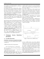
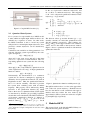
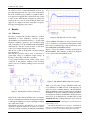
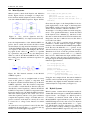
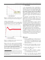
Quantised State System Simulation in Dymola/Modelica Using the DEVS Formalism
Quantised State System Simulation in Dymola/Modelica
using the DEVS Formalism
Tamara Beltrame
VTT, Industrial Systems
PO Box 1000, VM3
02150 Espoo, Finland
[email protected]
François E. Cellier
Institute of Computational Science
ETH Zurich
8092 Zurich, Switzerland
[email protected]
Abstract
Continuous-time systems can be converted to discreteevent descriptions using the Quantised State Systems
(QSS) formalism. Hence it is possible to simulate
continuous-time systems using a discrete-event simulation tool, such as a simulation engine based on the
DEVS formalism.
A new Dymola library, ModelicaDEVS, was developed that implements the DEVS formalism.
DEVS has been shown to be efficient for the simulation of systems exhibiting frequent switching operations, such as flyback converters. ModelicaDEVS contains a number of basic components that can be used
to carry out DEVS simulations of physical systems.
Furthermore, it is also possible - with some restrictions - to combine the two simulation types of ModelicaDEVS and Dymola (discrete-event and discretetime simulation) and create hybrid models that contain
ModelicaDEVS as well as standard Dymola components.
Keywords: DEVS formalism; Quantised State Systems; Event-Based Simulation; Numerical Integration
1 Introduction
of the new integration approach was to replace the
discretisation of time by a quantisation of state.
The DEVS formalism turned out to be particularly
well suited for implementing such a state quantisation
approach, given that it is not limited to a finite number
of system states, which is in contrast to many other
discrete-event simulation techniques.
The Quantised State Systems (QSS) introduced by
Kofman [6] in 2001 improved the original quantised
state approach of Zeigler by avoiding the problem of
ever creating illegitimate models, and hence gave rise
to efficient DEVS simulation of large and complex
systems.
The simulation of a continuous system by a (discrete) DEVS model comes with several benefits:
When using discretisation of time, variables have to
be updated synchronously1 . Thus, the time steps have
to be chosen according to the variable that changes the
fastest, otherwise a change in that variable could be
missed. In a large system where probably very slow
but also very fast variables are present, this is critical
to computation time, since the slow variables have
to be updated way too often. The DEVS formalism
however allows for asynchronous variable updates,
whereby the computational costs can be reduced
significantly: every variable updates at its own speed;
there is no need anymore for an adaptation to the
fastest one in order not to miss important developments between time steps. This property could be
extremely useful in stiff systems that exhibit widely
spread eigenvalues, i.e., that feature mixed slow and
fast variables.
The DEVS formalism is very well suited for problems
with frequent switching operations such as electrical
Since Dymola/Modelica was primarily designed to
deal with continuous physical problems, numerical
integration is central to its operation, and therefore,
the search for new algorithms that may improve the
efficiency of simulation runs is justified.
Toward the end of the nineties, a new approach for
numerical integration by a discrete-event formalism
has been developed by Zeigler et al. [13]: given
the fact that all computer-based continuous system
simulations have to undergo a discretisation of one
1 Note that this is not true for methods with dense output. Howform or another –as digital machines are not able ever, the above statement holds for the majority of today’s integrato process raw continuous signals– the basic idea tion methods, since they rarely make use of dense output.
The Modelica Association
73
Modelica 2006, September 4th – 5th
T. Beltrame, F.E. Cellier
external event has been received. δint (s) is the internal
transition that is executed as soon as the system has
spent in its current state the time indicated by the
time-advance function.
ta(s) is the so-called time advance function that
indicates how much time has to pass until the system
undergoes the next internal transition. The timeadvance function is often represented by variable σ
which holds the value for the amount of time that the
system has to remain in its current state in the absence
of external events.
The λ-function is the output function. It is executed
prior to performing an internal transition. External
transitions do not produce output.
Figure 1 illustrates the functioning of a DEVS model:
the system receives input (top graph) at certain time
Since the mid seventies, when Zeigler introduced the instants, changes its states according to the internal
DEVS formalism [11], there have emerged several and external transitions (center graph), and produces
DEVS implementations, most of them designed to output (bottom graph).
simulate discrete systems. However, one simulation/modelling software system aimed at simulating
continuous systems is PowerDEVS [8]: it provides
a library consisting of block diagram component
models that can be used for modelling any system
described by ODE’s (DAE’s), thereby allowing for the
simulation of continuous systems.
The implementation of ModelicaDEVS has been
kept close to the PowerDEVS simulation software. Hence ModelicaDEVS can be considered a
re-implementation of PowerDEVS in Modelica.
power systems. Given that the problem of iteration at
discontinuities does not apply anymore, it even allows
for real-time simulation.
For hybrid systems with continuous-time, discretetime, and discrete-event parts, a discrete-event method
provides a “unified simulation framework”: discretetime methods can be seen as a particular case of
discrete-event methods [6], and continuous-time parts
can be transformed in a straightforward manner to
discrete-time/discrete-event systems.
When using the QSS approach of Kofman in order to
transform a continuous system into a corresponding
discrete system, there exists a closed formula for the
global error bound [2], which allows a mathematical
analysis of the simulation.
2 Continuous
with DEVS
2.1
System
Simulation
The DEVS Formalism
Figure 1: Trajectories in a DEVS model.
The DEVS formalism has been introduced by Zeigler
in 1976 [11]. It was the first methodology designed
for discrete-event system simulation that is based on
In theory, DEVS models can describe arbitrarily
system theory.
complex systems. The only drawback is that the more
complex the system is, the more difficult it will be
A DEVS model has the following structure:
to set up the correct transition functions describing
the system. Fortunately, complex systems can be
M = hX,Y, S, δint (s), δext (s, e, x), λ(s),ta(s)i
broken down into simpler submodels that are easier to
where the variables have the following meaning (see handle. The fact that DEVS is closed under coupling
also [2], Chapter 11):
[2] makes such an approach viable.
X represents all possible inputs, Y represents the Figure 2 illustrates this concept: the model N consists
outputs, and S is the set of states.
of two coupled atomic models Ma and Mb . N can be
The variable e indicates the amount of time the system said to wrap Ma and Mb and is indistinguishable from
has already spent in the current state. δext (s, e, x) the outside from an atomic model.
is the external transition that is executed after an
The Modelica Association
74
Modelica 2006, September 4th – 5th
Quantised State System Simulation in Dymola/Modelica Using the DEVS Formalism
be the set of piecewise continuous trajectories, and
let x ∈ Ω be a continuous trajectory. The mapping
b : Ω → Ω is a hysteretic quantisation function if the
trajectory q = b(x) satisfies:

Qm
if t = t0



Qk+1 if x(t) = Qk+1 ∧ q(t − ) = Qk ∧ k < r
q(t) =
Q
if x(t) = Qk − ε ∧ q(t − ) = Qk ∧ k < 0


 k−1
−
q(t ) otherwise
and:
Figure 2: Coupled DEVS models [2].
2.2

 0 if x(t0 ) < Q0
r if x(t0 ) ≥ Qr
m=

j if Q j ≤ x(t0 ) < Q j+1
Quantised State Systems
For a system to be representable by a DEVS model,
it must exhibit an input/output behaviour that is describable by a sequence of events. In other words,
the DEVS formalism is able to model any system
with piecewise constant input/output trajectories, since
piecewise constant trajectories can be described by
events [2].
Continuous state variables are being quantised. Consider the following system represented by the statespace description:
ẋ(t) = f(x(t), u(t),t)
where x(t) is the state vector and u(t) is the input
vector, i.e. a piecewise constant function. The corresponding quantised state system has the following
form:
ẋ(t) ≈ f(q(t), u(t),t)
where q(t) is the (componentwise) quantised version
of the original state vector x(t). A simple quantisation
function could be:
q(t) = floor(x(t)).
Unfortunately, the transformation of a continuous
system into its discrete counterpart by applying an
arbitrarily chosen quantisation function can yield an
illegitimate model2 . Thus, the quantisation function
has to be chosen carefully, such that it prevents
the system from switching states with an infinite
fequency. This property can be achieved by adding
hysteresis to the quantisation function [6], which
leads to the notion of a Quantised State System (QSS)
as introduced by Kofman [6] providing legitimate
models that can be simulated by the DEVS formalism.
A hysteretic quantisation function is defined as
follows [2]: Let Q = {Q0 , Q1 , ..., Qr } be a set of real
numbers where Qk−1 < Qk with 1 ≤ k ≤ r. Let Ω
2 Definition
[2]: “A DEVS model is said to be legitimate if it
cannot perform an infinite number of transitions in a finite interval
of time.” Illustrative examples of illegitimate models can be found
in [2] and [6].
The Modelica Association
The discrete values Qi and the distance Qk+1 − Qk
(usually constant) are called the quantisation levels
and the quantum, respectively. The boundary values Q0 and Qr are the upper and the lower saturation
values, and ε is the width of the hysteresis window.
Figure 3 shows a quantisation function with uniform
quantisation intervals.
Figure 3: Quantisation function with hysteresis [2].
The QSS described above is a first-order approximation of the real system trajectory. Kofman however
has also introduced second- and third-order approximations that may reduce the error made by the
approximation. These systems are referred to as QSS2
[7] and QSS3 [9], respectively.
3
ModelicaDEVS
The average block of the ModelicaDEVS library exhibits the following basic structure:
75
Modelica 2006, September 4th – 5th
T. Beltrame, F.E. Cellier
1
2
3
4
5
6
7
8
9
10
11
12
13
14
15
16
17
18
19
20
21
22
23
24
25
26
27
28
29
30
31
32
33
34
by an equation
block SampleBlock
extends ModelicaDEVS.Interfaces. ... ;
parameter Real ... ;
dext = uEvent;
where uEvent is the Boolean component of the connector that represents an input event. Suppose now
that block A produces an output event at time t = 3.
At this precise instant, it updates its output vector with
the appropriate values (the coefficients of the Taylor
series) and sets A.yEvent to true:
protected
discrete Real lastTime(start=0);
discrete Real sigma(start=...);
Real e;
Boolean dext;
Boolean dint;
[...other variable declarations...]
when dint
yVal[1]=
yVal[2]=
yVal[3]=
end when;
yEvent =
equation
dext = uEvent;
dint = time>=pre(lastTime)+pre(sigma);
when {dint} then
yVal[1]= ...;
yVal[2]= ...;
yVal[3]= ...;
end when;
yEvent = edge(dint);
then
...; //new output value 1
...; //new output value 2
...; //new output value 3
edge(dint);
Still at time t = 3, block B notices that now B.uEvent
has become true (note that B.uEvent = A.yEvent
because the two blocks are connected), and therefore
dext has become true, also. Consequently, Block B is
executing its external transition [4].
when {dint, dext} then
e=time-pre(lastTime);
if dint then
[..internal transition behaviour..]
else
[..external transition behaviour..]
end if;
lastTime=time;
end when;
A DEVS model must contain code to perform
internal and external transitions, as well as execute the
time advance and output functions at the appropriate
instants. All of these functions have to be explicitly or
implicitly present in the ModelicaDEVS blocks.
The time advance function is normally represented
by a variable sigma. It is a popular trick in DEVS
end SampleBlock;
to represent the current value of the time advance
function by sigma [2].
The following sections will offer more insight into the The internal transition is executed when dint is true.
reasons for this specific block structure.
An internal transition depends only on sigma. Hence
the value of dint can be calculated as:
In accordance with the PowerDEVS implemen- dint = time >= pre(lastTime) + pre(sigma);
tation, ModelicaDEVS event ports (connectors) where lastTime holds the time of the last execution of
consist of four variables representing the coefficients a transition (internal or external).
to the first three terms (constant, linear, and quadratic) The external transition is executed when dext is true.
of the function’s Taylor series expansion, and a The variable dext is defined as follows:
Boolean value that indicates whether a block is
dext = uEvent;
currently sending an event.
The internal and external transitions are represented
Dense output can then be approximated as:
by a when-statement.
The reason for packing
yout = y0 + y1 · (t − tlast ) + y2 · (t − tlast )2
the internal and external transitions into a single
whereby the coefficient of the quadratic term of when-statement instead of having two separate whenthe Taylor series, y2 = yVal[3], is only used by statements, one representing the internal transition
the third-order accurate method, QSS3, whereas the and the lambda function, the other one representing
linear term, y1 = yVal[2], is used by QSS2 and QSS3. the external transition, is due to a rule of the Modelica
language specification that states that equations in
Let us now consider a small example in order to gain different when-statements may be evaluated simulincreased insight into the role of the Boolean variable taneously. Hence, if there are two when-statements
of the port. Let us assume a two-block system consist- each containing an expression for a variable X, X
ing of block A and block B, where the only input port is considered overdetermined. This circumstance
of block B is connected to the only output port of block would cause a syntactical problem with variables that
A. Every block features a variable dext accompanied have to be updated both during the internal and the
The Modelica Association
76
Modelica 2006, September 4th – 5th
Quantised State System Simulation in Dymola/Modelica Using the DEVS Formalism
external transition and thus would have to appear in
both when-statements. For this reason, we need to
have a when-statement that is active if either dint
or dext becomes true. Subsequently, an additional
discrimination is done within the when-statement,
determining whether it was an internal (dint is true)
or an external transition (dext is true) that made the
when-statement become active, and as the case may
be, updating the variables with the appropriate value.
The lambda function is executed right before an
internal transition. Lines 17-22 of the “block basic
structure” code (beginning of Section 3) constitute
the typical lambda function part, containing a whenstatement and a separate instruction for the yEvent
variable. The right hand side of the equations in the
lambda function normally depends on pre() values
of the used variables. This is due to the fact that
the lambda function has to be executed prior to the
internal transition. The variable yEvent has to be
true in the exact instant when an internal transition
is executed and false otherwise. This behaviour is
obtained by using the Modelica edge() operator.
There is one particular situation that can occur
in a model that requires special attention: let us
assume two connected blocks, where both block A
and block B have to execute an internal transition
simultaneously (Figure 4). Whereas block A simply
Figure 4: Concurrent events at block B.
executes its internal transition, block B is confronted
with the problem of concurrent events: from block
A it receives an external event, but at the same time,
it was about to undergo its own internal transition.
Which event should be processed first? This question
is to be answered by the priority settings between the
two blocks.
In our simple two-block example there are only
two possible priority orderings with the following
consequences: either block A is prior to block B, and
block A will produce the output event before block
B executes the internal transition (block B will first
execute an external transition triggered by the external
event it received from block A), or block B is prior
The Modelica Association
to block A, such that block B will first undergo its
internal transition and receive the external event right
afterwards, when A will be allowed to execute its
internal transition.
The problem of block priorities can be solved in
two ways: by an explicit, absolute ordering of all
components in a model (e.g., a list), or by letting
every block determine itself whether it processes the
external or the internal event first, in case both of them
occur simultaneously. ModelicaDEVS implements
the latter approach. As can be seen in the “block
basic structure” code, internal transitions take always
priority over external transitions (line 26: the code
checks first whether dint is true).
The reason for this choice is quite simple. As internal
events are processed before external events, and since
internal events are accompanied by output events,
the variable yEvent can be computed as a function
of dint alone. If we were to force external events
to be processed before internal events, we would
need to make sure that yEvent is only set true in the
case that the internal event is not accompanied by
a simultaneous external event. Thus yEvent would
now be a function of both dint and dext. Yet, dext
is a function of uEvent. Thus, if ModelicaDEVS
blocks were connected in a circular fashion, as this is
often the case, an algebraic loop in discrete (Boolean)
variables would be created, which would get the
Dymola compiler into trouble.
By forcing the internal events to always take preference over external events, ModelicaDEVS blocks
can be interconnected in an arbitrary fashion without
ever creating algebraic loops in the Boolean eventindication variables.
Note that since Dymola/Modelica is already aimed at
object-oriented modelling, which includes the reuse
of multi-component models as parts of larger models,
the issue of hierarchically coupled models did not
require any special treatment in ModelicaDEVS.
Dymola can trigger two types of events: state
events that require iteration to locate the event time,
and time events that make Dymola “jump” directly to
the point in time when the time event takes place.
The only expressions responsible for activating the
when-statements in the models, namely:
dext = uEvent;
and:
dint = time >= pre(lastTime) + pre(sigma);
both trigger time events and hence avoid the computationally more expensive state events.
77
Modelica 2006, September 4th – 5th
T. Beltrame, F.E. Cellier
An earlier version of ModelicaDEVS used an approach that triggered mostly state events. Inspired by
the book of Fritzson [4], a number of small modifications have been applied that converted all state events
to time events. Performance comparisons carried out
between the two versions showed that the time-event
approach is roughly four times faster than an equivalent approach triggering state events.
4 Results
4.1
Efficiency
In order to compare the run-time efficiency of ModelicaDEVS to other simulation software systems
(PowerDEVS and standard Dymola), a system with
frequent switching operations was modelled using
each of the three tools (PowerDEVS, ModelicaDEVS
and Dymola), and the execution times of the three
codes were compared against each other.
The chosen system is the flyback converter example
presented in [5].
The flyback converter can be used to transform a
given input voltage to a different output voltage. It
belongs to the group of DC-DC converters.
A very simple electrical circuit with a voltage source
connected to the primary winding of the converter
and a load to its secondary winding looks as shown in
Figure 5.
Figure 6: The flyback converter output.
or PowerDEVS, the behaviour of the converter needs
to be converted to a causalised block diagram3 , which
then can be modelled using component models of the
PowerDEVS/ModelicaDEVS libraries.
Figure 7 shows the flyback converter model built in
ModelicaDEVS. The structure of this block diagram
is also valid for the PowerDEVS model.
Figure 7: The ModelicaDEVS flyback converter.
Table 1 provides the average simulation CPU time
for a simulation of 0.002 seconds of the flyback converter model in standard Dymola, ModelicaDEVS,
and PowerDEVS, respectively. The Dymola and ModFigure 5: The flyback converter in Dymola.
elicaDEVS model were simulated setting the numerical integration method to LSODAR4 . Testing has been
Figure 6 shows the first two milliseconds of a simula- carried out on an IntelCeleron 2.6 GHz Laptop with
tion run of the flyback converter circuit given in Figure 256MB RAM. The resulting CPU time may vary from
3 For more details on the causalising process in the flyback con5. The rapid switching is a result of the high switching
rate of the ideal switch.
verter example, see [1].
4 Although ModelicaDEVS does not make use of LSODAR diThe flyback converter is described by a set of acausal
equations in Dymola. However, in order to be able to rectly, the event handling behaviour of Dymola is somewhat influmodel the flyback converter in either ModelicaDEVS enced by the selection of the numerical integration algorithm.
The Modelica Association
78
Modelica 2006, September 4th – 5th
Quantised State System Simulation in Dymola/Modelica Using the DEVS Formalism
one computer system to another, but the relative ordering is expected to remain the same.
Table 1: Execution efficiency comparison.
CPU
time
result
time [s] events points
Dymola
0.062
239
738
QSS1
3.55
6363 11829
M-DEVS QSS2
0.688
958
2299
QSS3
0.656
833
2164
QSS1
0.064
N/A
N/A
P-DEVS QSS2
0.019
N/A
N/A
QSS3
0.018
N/A
N/A
Table 1 shows a clear ordering of the three different
systems in terms of performance: PowerDEVS is
faster than Dymola, which in turn is faster than
ModelicaDEVS.
First, it needs to be remarked that standard Dymola
simulates this model very efficiently. The switching
(BooleanPulse) block leads to time events only,
whereas the diode should lead to state events. Yet, this
is not the case.
Switching at the input leads immediately to a switching of the diode as well. Since Dymola iterates after
each event to determine a consistent set of initial
conditions, the switching of the diode is accomplished
at once without need of first triggering a state event.
Second, the model is quite trivial. The execution
time is almost entirely dictated by the number of time
events handled. What happens in between events is
harmless in comparison.
Standard Dymola performs exactly one time event
per switching. In contrast, ModelicaDEVS performs
considerably more time events. Time events take here
the role of integration steps.
Figure 8 shows the constant term of the Taylor series
expansion of the load voltage as a function of time
for QSS1 and QSS3. QSS1 requires a new time event
as soon as the constant output no longer represents
the true output, whereas QSS3 requires an event
only, when the second-order accurate Taylor series
expansion no longer approximates the true output.
QSS1 requires roughly eight times as many events
as QSS3, and is therefore between five and six times
slower. Yet, even QSS3 requires roughly three times
as many events as standard Dymola. In addition, the
ModelicaDEVS model contains roughly three times
as many variables as the standard Dymola model.
All of these variables are being stored at every event.
Consequently, QSS3 is roughly nine times slower than
standard Dymola.
The Modelica Association
Figure 8: QSS3 simulation vs. QSS1 simulation.
Yet, QSS3 in PowerDEVS is roughly three times
faster than standard Dymola for comparable accuracy. A comparison between PowerDEVS and
ModelicaDEVS is not straightforward. PowerDEVS
implements Zeigler’s hierarchical simulator [12],
whereas ModelicaDEVS operates on simultaneous
equations and synchronous information flow [10].
Consequently, PowerDEVS suffers from requiring
message passing to implement the communication
between blocks, but enjoys the advantage of only
having to process those equations that are directly
involved with the event being handled. In contrast,
ModelicaDEVS needs to visit all equations of all
blocks whenever an event takes place. Which variables are to be updated in each case is decided by
Boolean expressions associated with the various
when-statements.
Yet the true difference in speed has probably more
to do with the event handling itself. Dymola has
been designed for optimal speed in the simulation
of continuous models and for optimal robustness in
handling hybrid models.
The algorithms implemented in Dymola for robust
event handling are important in the context of hybrid
modelling. In the context of a pure discrete-event
simulation, these algorithms are an overkill. For
example, in a pure discrete-event simulation there is
no need for iteration after each event to determine a
new consistent set of initial conditions. In Dymola,
many variables are being stored internally in order
to allow LSODAR to integrate continuous state
equations correctly across discontinuities. In a pure
discrete-event simulation, variables need to be stored
for output only.
79
Modelica 2006, September 4th – 5th
T. Beltrame, F.E. Cellier
4.2
Mixed Systems
du=der(u);
Mixed systems contain both Dymola and Modelica
blocks. Figure 9 shows an example of a simple electrical circuit modelled in Dymola, and in a mixed version with a ModelicaDEVS capacitor. Figure 10 illus-
Figure 9:
Two versions (Dymola and Dymola/ModelicaDEVS) of a simple electrical circuit.
trates the implementation of the ModelicaDEVS capacitor. On its outside, this block looks like a normal
electrical Dymola component, but internally it consists
of ModelicaDEVS blocks that model the behaviour
of a capacitor: The Gain block multiplies the incoming signal by the value of C1 , where C is specified
by a parameter, and passes it on to the Interpolator.
Taken as a whole, the ModelicaDEVS blocks constitute nothingR more than the well known capacitor formula v = C1 i dt.
when sample(start,period) then
yVal[1]=u;
yVal[2]=if method>1 then du else 0;
yVal[3]=if method>2 then der(du) else 0;
end when;
Given that the input of the SamplerTime block depends algebraically on the output of the Interpolator
in the DEVS capacitor, Dymola would have to differentiate discrete variables, which it is unable to do.
An attempt to solve this problem was made using Dymola’s “User specified Derivatives” feature described
in the Dymola User’s Manual [3]: functions for the
first and second derivatives have been inserted into the
Interpolator, but due to unknown reasons, this did not
resolve the issue either.
In order to be able to perform mixed simulations
nonetheless, another trick has been applied: supplementary to the standard ModelicaDEVS SamplerTime
block that uses the Modelica der() operator, an additional block has been programmed: the SamplerTimeNumerical block avoids the problem caused by
the der() operator by means of the delay() function
that is used to differentiate the input variable numerically. Instead of the first and second derivatives of
the input signal, the SamplerTimeNumerical returns a
numerical approximation:
Du = delay(pre(u),D);
D2u= delay(pre(u),2*D);
yVal[1]= pre(u);
yVal[2]= if method>1 then
(pre(u)-Du)/D else 0;
yVal[3]= if method>2 then
(pre(u)-2*Du+D2u)/(D*D) else 0;
Figure 10: The internal structure of the ModelicaDEVS capacitor.
Unfortunately, it is not as straightforward as it may
seem at first glance to replace a component from
the Dymola standard electrical library by its ModelicaDEVS equivalent: since the electrical components
do not assume a certain data flow direction (they are
described by acausal equations), whereas the ModelicaDEVS components do (DEVS components feature
input and output ports), the ModelicaDEVS capacitor
must turn acausal equations into causal ones. It assumes the capacitive current i to be given, and hence
computes the capacitive voltage v. Note that such a capacitor would not work anymore correctly if we were
to connect it to a voltage source instead of a current
source.
An even more severe problem is caused by the SamplerTime block applying the der() operator to the signal that it receives through its input port:
The Modelica Association
Using the new sampler block, the mixed simulation
could be carried out without any problems, and the results differ only slightly from the simulation with conventional Dymola components (see Figure 11).
4.3
Hybrid Systems
Hybrid systems contain mixed integration methods:
standard Modelica integrators and ModelicaDEVS Integrator blocks. An example of a hybrid system is
for instance an electrical circuit with at least one
ModelicaDEVS capacitor/inductor (using the ModelicaDEVS Integrator block) and at least one Dymola
capacitor/inductor (using the Modelica der() operator). The flyback converter of Section 4.1, where the
capacitor in the secondary winding is replaced by an
equivalent ModelicaDEVS capacitor, may serve as an
80
Modelica 2006, September 4th – 5th
Quantised State System Simulation in Dymola/Modelica Using the DEVS Formalism
5
Conclusions
A new Dymola/Modelica library implementing a
number of Quantised State System (QSS) simulation
algorithms has been presented. ModelicaDEVS duplicates the capabilities of PowerDEVS. The graphical
user interfaces of both tools are practically identical.
However, the underlying simulators are very different.
Whereas PowerDEVS implements Zeigler’s hierarchical DEVS simulator, ModelicaDEVS operates on
simultaneous equations and synchronous information
flows.
The embedding of ModelicaDEVS within the DyFigure 11: Standard Dymola (blue) and mixed (red) mola/Modelica environment enables users to mix
simulation of the simple electrical circuit (Figure 9).
DEVS models with other modelling methodologies
that are supported by Dymola and for which Dymola
offers software libraries.
example of a hybrid system.
Unfortunately, ModelicaDEVS is much less efficient
Note that the ModelicaDEVS capacitor applies numerin run-time performance than PowerDEVS. The loss
ical differentiation in order not to obtain “DAE index
of run-time efficiency is probably caused by Dymola’s
reduction” error messages (see previous section).
event handling algorithms that have been designed for
optimal robustness in the context of hybrid system
simulation rather than run-time efficiency in the
context of pure discrete-event system simulation.
Although ModelicaDEVS offers a full implementation
of a DEVS kernel and can therefore be used for the
simulation of arbitrary discrete-event systems, the
modelling blocks that have been made available so far
in ModelicaDEVS are geared towards the simulation
of continuous systems using QSS algorithms.
References
Figure 12: Standard Dymola (blue) and mixed (red)
simulation of the flyback converter.
Figure 12 shows the output of the mixed simulation
compared to the result of the standard Dymola simulation. Just as it was the case with the simpler example
of Section 4.2, the output of the hybrid simulation differs only slightly from the Dymola simulation.
Thus, it is also possible to perform not only accurate5
mixed simulations, but also hybrid simulations.
5 Note that due to the numerical differentiation used in the Sam-
plerTimeNumerical block, the result is not as accurate as if analytical differentiation had been used. However, the accuracy is sufficient for most purposes, and also adjustable through selection of
the width parameter, D.
The Modelica Association
81
[1] Beltrame, T. (2006), Design and Development of
a Dymola/Modelica Library for Discrete Eventoriented Systems using DEVS Methodology, MS
Thesis, Institute of Computational Science, ETH
Zurich, Switzerland.
[2] Cellier, F.E. and E. Kofman (2006), Continuous
System Simulation, Springer-Verlag, New York.
[3] Dynasim AB (2006), Dymola Users’ Manual,
Version 6.0, Lund, Sweden.
[4] Fritzson, P. (2004), Principles of ObjectOriented Modeling and Simulation with Modelica 2.1, Wiley-Interscience, New York.
[5] Glaser, J.S., F.E. Cellier, and A.F. Witulski
(1995), “Object-Oriented Switching Power ConModelica 2006, September 4th – 5th
T. Beltrame, F.E. Cellier
verter Modeling Using Dymola With EventHandling,” Proc. OOS’95, SCS Object-Oriented
Simulation Conference, Las Vegas, NV, pp.141146.
Biographies
Tamara Beltrame received her
MS degree in computer science
from the Swiss Federal Institute
of Technology (ETH) Zurich in
2006. She recently started working
at VTT (Finland), where she deals
with problems of simulation aided
automation testing.
[6] Kofman, E. and S. Junco (2001), “Quantised
State Systems: A DEVS Approach for Continuous Systems Simulation,” Transactions of SCS,
18(3), pp.123-132.
[7] Kofman, E., “A Second Order Approximation for
DEVS Simulation of Continuous Systems,” Simulation, 78(2), pp.76-89.
[8] Kofman, E., M. Lapadula, and E. Pagliero
(2003), PowerDEVS: A DEVS-based Environment for Hybrid System Modeling and Simulation, Technical Report LSD0306, LSD, Universidad Nacional de Rosario, Argentina.
[9] Kofman, E., “A Third Order Discrete Event
Method for Continuous System Simulation,”
Latin American Applied Research, 36(2),
pp.101-108.
[10] Otter, M., H. Emqvist, and S.E. Mattsson (1999),
“Hybrid Modeling in Modelica Based on the
Synchronous Data Flow Principle,” CACSD’99,
IEEE Symposium on Computer-Aided Control
System Design, Hawaii, pp.151-157.
[11] Zeigler, B.P. (1976), Theory of Modeling and
Simulation, John Wiley & Sons, New York.
[12] Zeigler, B.P. (1984), Multifacetted Modelling
and Discrete Event Simulation, Academic Press,
London.
[13] Zeigler, B.P. and J.S. Lee (1998), “Theory of Quantized Systems: Formal Basis for
DEVS/HLA Distributed Simulation Environment,” SPIE Proceedings, Vol. 3369, pp.49-58.
The Modelica Association
François E. Cellier received his BS
degree in electrical engineering in
1972, his MS degree in automatic
control in 1973, and his PhD degree in technical sciences in 1979,
all from the Swiss Federal Institute
of Technology (ETH) Zurich. Dr.
Cellier worked at the University of
Arizona as professor of Electrical and Computer Engineering from 1984 until 2005. He recently returned to
his home country of Switzerland. Dr. Cellier’s main
scientific interests concern modeling and simulation
methodologies, and the design of advanced software
systems for simulation, computer aided modeling, and
computer-aided design. Dr. Cellier has authored or coauthored more than 200 technical publications, and he
has edited several books. He published a textbook on
Continuous System Modeling in 1991 and a second
textbook on Continuous System Simulation in 2006,
both with Springer-Verlag, New York. He served as
general chair or program chair of many international
conferences, and serves currently as president of the
Society for Modeling and Simulation International.
82
Modelica 2006, September 4th – 5th