1
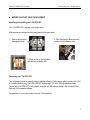
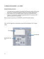
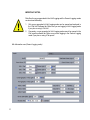
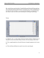
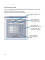
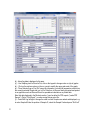
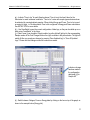
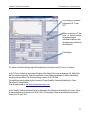
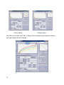
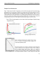
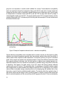
I-CAL 2000 HPC
User Manual
Calmetrix I-Cal 2000 HPC User Manual
CALMETRIX INC.
I-CAL 2000 HPC ISOTHERMAL CALORIMETER
FOR CONCRETE AND CEMENT
USER MANUAL
2
Calmetrix I-Cal 2000 HPC User Manual
© 2016 Calmetrix Inc. – All rights reserved
IMPORTANT SAFETY RULES
•
Exercise caution when lifting the calorimeter to avoid back or other
injuries. Consider a two person lift or mechanical aid.
•
Never operate the calorimeter or temperature control unit in a wet
environment.
DISCLAIMER
Calmetrix does not assume any liability as related to the accuracy, relevance or interpretation of results
while using I-Cal or the CalCommander software.
COPYRIGHT
This User Manual is subject to copyright and may not be reproduced in whole or part without permission.
3
4
Calmetrix I-Cal 2000 HPC User Manual
© 2016 Calmetrix Inc. – All rights reserved
TABLE OF CONTENTS
__________
A.
BEFORE YOU START USING THE EQUIPMENT ………………………………….
Page 7
B.
GENERAL USE ………………………………………………………………………….
Page 8
C.
HANDLING INSTRUCTIONS …………………………………………………………..
Page 9
D.
CALIBRATION……………………………………………...........................................
Page 9
E.
OPERATING YOUR EQUIPMENT – I-CAL LOGGER ………………………………
Page 10
F.
SAMPLE PREPARATION AND RECOMMENDED TEST PROCEDURE ………..
Page 17
G. VISUALIZING RESULTS – I-CAL REPORTS ………………………………………..
Page 20
H.
DETERMINING ACTIVATION ENERGY – I-CAL AE………………………………..
Page 25
I.
PREDICTING COMPRESSIVE STRENGTH – I-CAL STRENGTH………………..
Page 33
J.
ESTIMATING SETTING TIMES – I-CAL SET ……………………………………….
Page 39
K.
DETERMINING HEAT OF HYDRATION – I-CALHoH ………………………………..
Page 43
5
6
Calmetrix I-Cal 2000 HPC User Manual
A.
© 2016 Calmetrix Inc. – All rights reserved
BEFORE YOU START USING THE EQUIPMENT
Unpacking and Installing your I-Cal 2000 HPC.
Your I-Cal 2000 HPC is shipped in one single carton.
All accessories are included in white boxes placed in the main carton.
1.
Remove all protective
packaging material.
1.
2. Place the stacks of three reference
masses into the reference cells
3. Place the lids on the reference
cells and active sample cells.
Connecting your I-Cal 2000 HPC.
Your calorimeter includes a computer with pre-installed software. Use the power cable to connect your I-Cal
to a suitable electrical plug. Your I-Cal 2000 HPC functions with 110-240V, 50/60 Hz electrical supply.
Connect your I-Cal 2000 HPC to the computer using the two USB cables included in the Accessories box.
Open the CalCommander software.
Congratulations! You are now ready to use your I-Cal equipment.
7
Installing the CalCommander Software on additional computers.
Minimum requirements: Windows XP or later, 2 GB RAM and 250MB hard drive space, screen resolution of
1024x768 or higher.
Do not yet connect your I-Cal unit to the new computer. Install your software first:
1.
2.
3.
4.
Insert the Calmetrix USB Flash Drive in your computer’s USB port and browse to the Software
Installation folder. Double-click on the CalCommSetup icon and follow the on-screen installation
instructions. Refer to detailed instructions on the Quick Set-Up sheet enclosed in the Accessories
box. Do not restart the computer during installation, even if prompted to do so.
Once the installation is finished, connect your I-Cal 2000 HPC and wait for 30 seconds for the
operating system to recognize the equipment. Then open CalCommander.
Click on the Settings tab
Email your ID number to [email protected] or call +1 617-203-2090 to obtain your
Registration number. Once received, key in the number in the Reg ID field.
NOTE: in addition to the pre-installed software on the computer that came wit your I-Cal 2000 HPC,
your I-Cal 2000 HPC includes one free software license for the I-Cal Logger logging interface, one
license for the I-Cal Reports report generator and one license for the I-Cal HoH heat of hydration
software. The computer you register for the use of your I-Cal will be the only computer registered. To
purchase additional licenses, please email [email protected] or call (617) 203-2090.
5.
6.
Once you received your 7-digit registration numbers for I-Cal Logger, I-Cal Reports, I-Cal HoH, and
any additional modules you purchased, enter them in the Settings tab.
Once the registration numbers have been keyed in, the corresponding boxes should be checked.
You are now ready to use your I-Cal 2000 HPC on the new computer.
B. GENERAL USE
Calmetrix I-Cal calorimeters measure the heat flow from concrete, mortar or cement paste samples over
time in a close to constant temperature environment. The heat flow curve provides a “fingerprint” of the
chemical reactions in the sample. We recommend that you review ASTM C1679 general practice before
using your calorimeter.
8
Calmetrix I-Cal 2000 HPC User Manual
© 2016 Calmetrix Inc. – All rights reserved
C. HANDLING INSTRUCTIONS
The reusable plastic sample cups must be clean on the outside before inserting them into the calorimeter.
Cement or admixtures on the outside will cause vials to get stuck in the calorimeter, with expensive and
time-consuming repair as a result. Cups must be properly sealed to avoid erroneous measurement data.
Only use the Suction Cup that was provided with your I-Cal calorimeter to remove Plastic Cups from the
unit. Other removal methods may damage the unit or cause sample material to spill.
When opening the lid while performing a test, immediately close the lid when finished to minimize heat
exchange caused by keeping the lid open.
Use gloves and paper towels to ensure NO admixtures, cement dust, fingerprints or other material get left on
the outside of sample cups when loading them into the calorimeter.
D. CALIBRATION
Your I-Cal calorimeter was calibrated before shipping. You do not need to recalibrate the equipment. The
calibration file is already placed in the computer that was shipped with your I-Cal equipment. The calibration
file is placed in C:\Users\Public\Documents\Calmetrix\CalCommander\Calibration and can be copied to
another computer you use to operate your equipment. Always make sure that the Yellow Calibration light is
lit on the upper right hand side of the I-Cal Logger screen when operating your equipment, as shown in Part
E. “Operating your Equipment – I-Cal Logger” below.
Please email us at [email protected] or call +1 617-203-2090 for any help with calibration and
calibration files.
9
E. OPERATING YOUR EQUIPMENT – I-CAL LOGGER
Important Operating instructions.
•
•
Your computer has to be connected to the equipment at all times while running a test. Do not plug
and unplug your I-Cal while CalCommander is running, as this will cause the program to fail
While running a test, the CalCommander software is continuously communication with the
equipment. It is recommended to disable all energy saving features of the computer to avoid
possible interruption in the communication
With your computer connected to your I-Cal 2000 HPC, open the CalCommander software
Click on the I-Cal Logger tab on top and familiarize yourself with the main window of the I-Cal Logger
module:
Plot area
Command area
Mix Information area
area
10
Calmetrix I-Cal 2000 HPC User Manual
© 2016 Calmetrix Inc. – All rights reserved
Command area.
This area is used to operate the I-Cal’s logging functions
Select output to plot: Voltage is raw data measured by heat sensors. Power
is heat flow normalized per unit of dry cement or cementitious material.
Energy is accumulated heat per unit of dry cement or cementitious material.
Detects if a Calibration file is present. A Green indicator means that the
Calibration file is present and loaded. If the indicator is Red, locate and
install the Calibration file as in Section D of this Manual
Voltage: real-time measurement by sensor.
Status: yellow with time if logging is active, gray if logging is inactive.
Last logged: displays last value logged by sensor
Choose between two ways to log data:
a. select HoH Logging if you would like to determine the absolute heat of
hydration value, for example according to ASTM C1702. In HoH Logging
mode, you can choose a logging interval for an Initial Phase, and a another
usually longer interval after the Initial Phase of hydration. Refer to ASTM
C1702 for guidance on logging intervals
b. select Generic Logging for all other experiments
Control the temperature in your calorimeter.
Set T env: enter desired test temperature between 5°C and 45°C and press
“Turn Controller ON”. Remember to set the desired temperature and let the
equipment stabilize to isothermal conditions for at least 24 hours before
testing begins.
Actual T env: actual temperature inside the calorimeter.
Copy/Paste functions for data contained in the Mix Configuration area.
These commands facilitate copying a mix configuration from one channel to
another. Configuration Templates are for frequently used mixes. Press
Update Configuration to save any changes to configuration data.
Start logging each channel as close as possible to the time when water enters
in contact with the cement.
Stop logging the selected channel – you can stop an experiment at any time up
to the logging time defined in (b).
11
IMPORTANT NOTES:
Data files for curves generated in the HoH Logging and the Generic Logging modes
are structured differently:
1.
2.
Only curves generated in HoH Logging mode can be opened and analyzed in
the I-Cal HoH Software tab. Make sure you are logging in HoH Logging mode
if you plan on using I-Cal HoH
Conversely, curves generated in HoH Logging mode cannot be opened in the
I-Cal reports software tab. Make sure you are logging in the Generic Logging
mode if you plan on using I-Cal reports
Mix Information area (Generic Logging mode)
(f)
(d)
(e)
(a)
(g)
(b)
(c)
12
Calmetrix I-Cal 2000 HPC User Manual
© 2016 Calmetrix Inc. – All rights reserved
Box (a) – Total Mass – enter the total mass of specimen as sampled. Target ~20-50 g for cement paste,
100 g for mortar and a full cup for concrete. This information is used to normalize readings across
samples. Please note that units (US or metric system) can be changed in the Settings tab
Box (b) – Logging, hh:mm – enter the desired total length of the experiment
Box (c) – Mix Date/Time – enter the mixing time (when the water gets in contact with the cement). Make
sure you fill in this part properly, as the mix time is used in all other software tabs to display and analyze
data properly
Box (d) – Content, SCM 1, 2 &3 - Enter SCM unit mass as per mix design. This mass is regarded as a
“filler” (inert material) if plotting Power per unit of dry cement and considered “active” if plotting Power
per unit of dry cementitious material. You MUST enter the data for each SCM if included in the
sample in order to be able to plot Power per Unit later.
Box (e) – Content, Coarse and Fine Aggregate - Enter coarse and fine aggregate mass per mix design
if testing mortar or concrete. (Do not enter coarse aggregates if these have been removed from mix
prior to sampling). As with SCMs, you MUST enter data for coarse and fine aggregate if included in
sample
Box (f) – Total Water Content and Total Cement Content – Enter data as per your mix design (cement
content and total water to reach the design water cement ratio)
Box (g) – Admixture data – These fields are for informational purposes only. The values are not used in
any calculations. Add any aqueous part of admixtures to the Total Water Content (f).
Note that for boxes (a), (d) and (f), you can use the proposed units or any other unit (e.g. grams of each
material you used when preparing your sample on a benchtop mixer), as long as you use the same
units for all these fields.
The total mass in box (a) has to be expressed in grams, as it is used to compute and display Power and
Energy per unit weight of material.
13
Mix Information Area (HoH Logging mode)
(a)
(b)
(c)
(f)
(g)
(d)
(h)
(e)
Box (a) – Water Content – Enter the total water content contained in your sample
Box (b) – Cement or Inert Content – Enter the total mass of cement (if logging an active sample) or of
inert material (if logging a reference sample to determine the Q3 correction factor as per ASTM C1702).
Box (c) – SCM content – Enter the total mass of Supplementary Cementitious Material contained in
your sample
Box (d) and (e) – Total Mass and Water/Binder Ratio are calculated values
Box (f) – Mix Date / Time – Make sure to enter the mix time, when water gets in contact with the cement
Box (g) – Indicate the Mixing Method, if applying ASTM C1702
Box (h) – Logging time – A typical heat of hydration test should last 168 hours or more. Please enter a
value that allows for at least 168 hours of logging from Mix time
14
Calmetrix I-Cal 2000 HPC User Manual
© 2016 Calmetrix Inc. – All rights reserved
Note: raw data files are saved in the folder C:\Users\Public\Documents\Calmetrix\CalCommander\Logs
once a measurement has been finished and saved. This allows the user to correct mix design data until
the measurement has been finished. You can also copy finished data sets to your designated network
drive. Be sure to create a sub-folder for each individual project to facilitate good record keeping.
Plot area.
(c)
(b)
(a)
(a)
(a) - Right-click on the x or y-axis to change scaling from Automatic to Manual. In Manual mode, you
can adjust the min and max by double-clicking on a number on the axis and typing in desired values .
(b) - Click on a graph legend/color on the right of the screen to change the appearance (color, line type,
etc.).
(c) - Click on the Zoom and Motion tools on top (f) to zoom in/out or move the graph.
15
Units and Channel Color Coding.
Units (metric or standard US) and colors assigned to the curves corresponding to each test channel can be
modified in the SETTINGS tab. Click on a color to change it.
Make sure to press “Apply New Settings” to save any changes.
Change units from Metric to US
Click on a default color to
change and select a new
color in the pop-up window.
Select or deselect the
Software application tabs you
would like to show in the tab
list on the top of the window.
Click on a “Apply New
Settings” to validate your
changes.
16
Calmetrix I-Cal 2000 HPC User Manual
© 2016 Calmetrix Inc. – All rights reserved
F. SAMPLE PREPARATION AND RECOMMENDED TEST PROCEDURE
1.
Ensure that the mixing procedure is sufficient to disperse binder properly.
2.
If the w/c ratio is pre-defined, perform a pre-test mix with blank cement paste or mortar (no
admixtures) and another pre-test with the highest desired dosage of admixtures. Adjust w/c ratio if
necessary.
3.
If the water demand of the cement – admixture combination to be tested is unknown, perform a pretest to determine required water to binder ratio (binder comprises of cement and any pozzolan used
as cement replacement)
How to accommodate different sample sizes of mortar, concrete or paste.
I-Cal 2000 HPC is equipped with variable reference cells to accommodate different sample sizes and types
in the sample cells. You can use either one, two or three of the supplied metal references, or use any
custom made reference such as a sample of inert sand. In general, the thermal mass of the reference
should be similar to that of the sample. The table below serves as a guide for using the supplied metal
references:
Sample type
Reference
20-100 g cement paste
1 metal cylinder
100-200 g cement paste or mortar
2 metal cylinders
250+ g cement paste, mortar or concrete
3 metal cylinders
Metal
references
Reference Cell
Sample to be tested
17
Recommended preparation of cement paste, mortar or concrete samples.
4.
Dial in desired test temperature in the “Set Tenv” box in the I-Cal Logger tab and press Turn
Controller On. The controller should be on for at least 24 hours before test runs to reach a stable test
temperature.
5.
Pre-dilute admixtures to ensure accurate weighing or use high accuracy micro-pipettes for accurate
volumetric dosing.
6.
If the mixing procedure is new to the operator, run 5-10 practice mixes to ensure a consistent mixing
method throughout a test series.
7.
Use the same mixing sequences and times as far as possible within a test series
8.
Prepare mortar or concrete according to standard. For a better signal to noise ratio, you can remove
the coarse aggregates > 4 mm using a sieve. Be sure to enter all the different materials used in the
software to ensure proper calculation of power and heat. The software reports power and heat
normalized to total weight of cementitious materials or portland cement, making it easy to visualize
any effect of admixtures and SCM’s on the portland cement reaction. Please be careful not to spill
any material outside of the 125 ml sample cup.
9.
For paste calorimetry, several methods ca be used, including hand mixing and using a benchtop
mixer. You can visualize a video tutorial on the Calmetrix website, in the Support Section.
The following procedure is commonly used by operators of Calmetrix I-Cal calorimeters:
18
a)
Weigh up 100 grams of cement in a plastic 800ml beaker and cover.
b)
Place a clean empty specimen cup onto the scale and weigh out the required amount of
admixture
c)
Add water and diluted admixture for mix water addition to bring the total weight to 45
grams (for a W/C of ratio of 0.45). Immediately start the logger for this cell.
Calmetrix I-Cal 2000 HPC User Manual
© 2016 Calmetrix Inc. – All rights reserved
d)
Use a commercial laboratory mixer at a speed of 400 rpm for 4 minutes after the addition
of the water. Delayed addition admixtures are added at the 60-second mark and mixed for
the remaining 3 minutes. Tail End addition admixtures are added at the 15-second mark
and mixed for the remaining 3 minutes and 45 seconds Note that mix water must be
adjusted for any water in the admixture as the water to cement ratio is kept constant
unless otherwise requested.
e)
Place an empty clean 125 ml plastic cup on the scale and tare. Carefully weigh out
approximately the paste amount required to reach 25 grams of paste. You must be
careful not to get any paste outside of the 125 ml sample cup. Record the total mass
of the sample and update in the Mix Configuration part on the I-Cal tab in CalCommander.
f)
Quickly place the plastic lid on the sample cup and make sure cup is perfectly clean and
sealed.
g)
Target the same time between start of mixing (i.e. when cement and water get in contact)
and loading into the calorimeter for all mixes in a test series.
19
G. VISUALIZING RESULTS – I-CAL REPORT GENERATOR
Using I-Cal Reports to plot and interpret data or create reports.
With CalCommander open on your computer, click on the I-Cal Reports Tab on top.
appears, as in the picture below.
A new window
(a3)
(a1)
(a2)
(a1) Open Data Folder – this command is a direct link to open the Calmetrix folder on your computer,
which contains the default folders where data logs, images, batches and reports are stored.
(a2) Load Batch – lets you load a combination of data logs that you previously saved as a Batch
(using the Save Batch command). This lets you load sets of curves from previous work with I-Cal
Reports, saved as batches, without having to import individual logs one by one.
20
Calmetrix I-Cal 2000 HPC User Manual
© 2016 Calmetrix Inc. – All rights reserved
(a3) - Add Logs – lets you load data logs from completed tests. A new window will appear.
Browse to the folder where you stored your completed test file data.
Select the logs you would like to import. For multiple selections, press the <CTRL> key while
selecting.
Repeat the steps above to add more files form other log files. You can add up to 8 files on any
Report Generator graph.
Click OK and the files you selected will appear in the Report Generator window.
21
(k)
(d)
(c)
(b)
(d)
(d)
(g)
(i)
(e)
(f)
(h)
(b) - Actual log data is displayed in this area.
(c) - Use Graphing tools to Zoom In/Out, click on the legend to change colors or style of graphs.
(d) - Click on the min/max values on the x or y-axis to modify the range and scale of the graph.
(e) - “Save Selected Log as Text File” saves the information, including all temperature values from
the currently selected Sample tab in a .txt file. Data from .txt files can easily be copied and pasted
in an application such as Microsoft Excel for spreadsheet calculations on plotted data.
Note that data displayed in the Mix data section (i) can be edited for PDF reports (“create PDF
Reports”), Prints (“Print Report”), or when saving data as a text file.
(f) – Press Shift Log left/right to change the order in which Samples are ranked and displayed, e.g.
to make Sample #2 take the position of Sample #1, select the Sample 2 tab and press “Shift Left”
22
(e)
Calmetrix I-Cal 2000 HPC User Manual
© 2016 Calmetrix Inc. – All rights reserved
(g) – Indicate “Time to Iso” for each Sample channel. Time to Iso is the time it takes for the
calorimeter to reach isothermal conditions. “Time to Iso” varies with sample type and size and can
be estimated by running duplicate samples. When plotting Energy and Power, Time to Iso is used
as a point of origin, i.e. all values before Time to Iso are ignored in Energy and Power calculations.
See ASTM C1679 for more details.
(h) – Use Save Batch to save the current configuration of data logs, so they can be called up as on
batch using “Load Batch” in the future.
(j) – Data in area (j) can be edited. If data is edited, a yellow light will light up for the corresponding
Sample number in the Conf Changed field on the right, as shown in the picture below. The light will
switch off after you saved your changes by pressing “Save Updated Log” or “Save All Updated
Logs”. Please note that changes cannot be undone once saved.
Indicates a change
has been made in
the configuration
data [area (j)] for
Sample # 4
(i)
(k) - Switch between Voltages, Power or Energy data by clicking on the box on top of the graph, as
shown in the example below (Energy plot).
23
For examples and guidance on interpretation of results, it is highly recommended to obtain a copy of
Standard Practice C1679 from ASTM and review the examples of interpretation given in the appendix
of this standard.
Calmetrix does not warrant the fitness for purpose of any equipment, software, training or other commercial
and non-commercial products marketed, distributed or recommended by Calmetrix, its principals, employees
and other representatives. Calmetrix does not assume any liability as related to the accuracy, relevance or
interpretation of results while using I-Cal and CalCommander.
24
Calmetrix I-Cal 2000 HPC User Manual
© 2016 Calmetrix Inc. – All rights reserved
H. DETERMINING ACTIVATION ENERGY – I-CAL AE (Optional Module)
What is Activation Energy?
The temperature dependency of the hydration rate of portland cement can be described by Arrhenius’ law,
with faster hydration the warmer the concrete. See equation (1) where
(1)
k is the rate constant for the reaction, Z is a proportionality constant that varies from one reaction to another.
Ea is the activation energy for the reaction, which in case of most cementitious systems is the so-called
“apparent” activation energy, since several complex chemical reactions may take place during the hardening
process. R is the ideal gas constant in joules per mole Kelvin, and T is the temperature in Kelvin. According
to this equation, a plot of ln k versus 1/T should give a straight line with a slope of - Ea/R. The calculation of
the apparent activation energy is based on the assumption that the overall reaction proceeds along the
same path at different temperatures according to the Arrhenius law. It is assumed that the activation energy
is only dependent on the produced energy (the degree of hydration), and therefore the activation energy can
be evaluated at different degrees oh hydration from the slope of the logarithm of the thermal power vs. the
inverse of the absolute temperature.
How to use the I-Cal AE module.
To utilize the Activation Energy module, you will need to run tests at at least three different temperatures for
any given mix.
CalCommander uses two different methods to determine activation energy: the “S-shaped” method
developed by Anton Schindler and the “Generic” method developed by Lars Wadso. While there is no strict
guideline as to which method is best, in general terms, we recommend use of the “S-shaped” method for
mixes where Portland cement is the predominant cementitious material, and the ”Generic” method for very
high substitution levels or geopolymer–type mixes.
In the Setting tab, choose the method you would like to use. Once selected, make sure you press “Apply
New Settings” for the change to take effect:
25
Now click on the I-Cal AE tab on top. The following window will appear.
Click add Logs to add test results from tests conducted at three (or more) different temperatures for the
same mix.
26
Calmetrix I-Cal 2000 HPC User Manual
© 2016 Calmetrix Inc. – All rights reserved
In this example, tests were
performed at 50, 73 and
95°F.
Make sure you key in “Time
to Iso”, i.e. the time at which
the system reached
isothermal conditions, after
the sample was inserted into
the calorimeter.
Click Analyze
The values of Activation Energy might differ depending on the method used (“S-Curve” or Generic”).
In the “S-Curve” method, several values indicative of the shape of the curve are displayed: Hu, Alpha, Beta
and Tau values are inputs for Texas ConcreteWorks.,a free software application for maturity calculations,
including crack prediction. The Activation Energy is shown in the “AE” field.
ConcreteWorks was developed by the University of Texas Durability Center and funded by the Texas
Department of Transportation.
It can be downloaded at: http://www.texasconcreteworks.com
In the “Generic” method, Activation Energy is calculated at five different points along the test curves. Values
for these calculations are shown in the “E act” fields. The average of these values should be used, and is
shown in the “E aver” field.
27
“Generic” method
“S-shape” method
At any time, you can switch from “Power” to “Energy” plots by selecting the type of graph from the drop
down menu located at the top of the graph.
28
Calmetrix I-Cal 2000 HPC User Manual
© 2016 Calmetrix Inc. – All rights reserved
Examples of use of Arrhenius plots.
Figure 1 below shows the effect of temperature on the heat flow rate (power) and the produced energy
(approximation for the overall degree of hydration) for a portland cement paste without admixture, w/c 0.45.
Note that the initial non-isothermal heat flow is excluded from the energy calculation, Figure 1 (b). The
measured data was then fitted mathematically to an S-shaped hydration development curve that is known to
work well for portland cement based mixtures according to Schindler (Ref 1 & 2 below). Figure 2 shows the
corresponding Arrhenius plot as a fitted straight line representing the apparent activation energy.
Figure 1: Effect of curing temperature on rate of reaction (heat flow) and degree of hydration (energy
– integrated heat flow)
(a) Heat flow
(b) Energy (integrated heat flow)
Figure 2: Arrhenius plot based on the results in Figure 3 using
Eqv (1). The slope is the apparent activation energy for the
overall cement hydration process.
Arrhenius law applies only if a change in temperature merely changes the
speed of reaction and not the major path of reaction. This is usually the
case for straight portland cement mixtures, which in turn makes the
foundation for the use of Maturity models for predicting degree of hydration
and strength development. However, a “major” change in the reaction path
29
going from one temperature to another would invalidate this concept. Cement-admixture incompatibility
issues are sometimes induced by a temperature change such that the major path of cement reaction has
changed and therefore could be undetected by standard laboratory room temperature tests. Figure 8 shows
an example where an industrial concrete with 20% fly ash and 0.3% low range water reducer by weight of
cement hydrated normally at 10 and 23°C. The slower hydration rate at 10°C is expected, however note the
complete different path at 40°C as evident by both the timing and abnormal shape of the main exotherm and
the abnormal Arrhenius plot.
(a) Heat flow
(b) Arrhenius plot
Figure 3: Example of temperature induced cement – admixture incompatibility
Cement-admixture incompatibility issues associated with hot weather concrete are often based on sulfate
imbalance, since higher temperatures generally make the aluminate reactions faster while the solubility of
calcium sulfate is lower compared to lower temperatures. The response (red curve) in Figure 3 is somewhat
typical. As the concrete was mixed at room temperatures before curing at three different temperatures inside
three separate isothermal calorimeter units, the initial positive or negative power readings represent nonisothermal conditions and are not included in the calculation of activation energy, along with the initial heat
of dissolution. Note however the higher activity of the 40°C sample after having reached isothermal
conditions after some 60 minutes. The accelerating effect of temperature on aluminate hydration coupled
with a negative effect on gypsum solubility likely caused the mixture at 40°C to temporarily run out of soluble
calcium sulfate at early age, causing a poisoning effect on the strength-giving alite hydration that is often
observed as a result of poorly controlled aluminate hydration. The alumina activity then reached a stage of
lower activity which was low enough to allow for enough gypsum to dissolve to reach sulfate balance and
allow for some alite hydration until the mix most likely ran out of gypsum after about 18 hours as indicated by
30
Calmetrix I-Cal 2000 HPC User Manual
© 2016 Calmetrix Inc. – All rights reserved
the very steep exotherm. The steep slope and amount of heat released by this exotherm is typical of uncontrolled alumina hydration, which in turn effectively poisoned any further alite hydration during the test.
The sample cured at 40°C was soft without any appreciable mechanical strength at the end of the test,
which is also typical for the type of response seen by calorimetry at 40°C (red curve).
Not all cases of non-compliance with Arrhenius law are as clear-cut as the example shown in Figure 3.
Figure 4 shows an example of alkali activated fly ash concrete where the power plots have somewhat
different shape at 40°C relative to 23 and 10°C. The different shape seen by calorimetry at 40°C may
indicate a partially different reaction path or possibly an added reaction at high temperature, while the
Arrhenius plot assumes that the path of reaction is the same at all temperatures. In other words it is
assumed that the reaction taking place in the second peak that was only observed at 40°C is similar to the
reaction taking place in the first peak at all three temperatures. More knowledge is needed about the general
hydration mechanism before one can assume that the activation energy concept is valid and useable for
predicting engineering properties such as strength development before applying it to novel binders such as
alkali activated fly ash. Nevertheless, calorimetry is a very useful tool for characterizing the reactivity of both
conventional and non-conventional binder systems to identify areas of potential concern for the practitioner
as well as where more work is needed for the researcher.
(a) Heat flow
(b) Arrhenius plot
31
References:
32
1.
Schindler, A.K. and Folliard, K.J., “Heat of hydration models for cementitious materials,” ACI Mat.
Journal., V. 102, No. 1, pp. 24-33, 2005.
2.
Schindler, A.K., “Effect of temperature on hydration of cementitious materials,” ACI Mat. Journal.,
V. 101, No. 1, pp. 72-81, 2004.
3.
Riding, K.A., Poole J.L., Juenger, M.C.G., Schindler, A.K., and Folliard K.J., “Calorimetry
Performed On-Site: Methods and Uses”, ACI SP-241.
4.
Poole, J.L., “Hydration Study of Cementitious Materials Using Semi-Adiabatic Calorimetry,” PhD
Dissertation, The University of Texas at Austin, Austin, TX, 2007.
Calmetrix I-Cal 2000 HPC User Manual
© 2016 Calmetrix Inc. – All rights reserved
I. PREDICTING COMPRESSIVE STRENGTH DEVELOPMENT – I-CAL STRENGTH (Optional Module)
I-Cal Strength is based on the assumption that for a given mix design with a given porosity there is a
correlation between the energy released (degree of hydration) and the compressive strength development.
As with traditional maturity, the assumption is only valid for mixes with the same materials and proportions.
How to use the I-Cal Strength module.
To be able to predict compressive strength development for a given mix design, you will first have to create
a model which establishes the relationship between degree of hydration and compressive strength.
IMPORTANT NOTE: Any given model is only valid for prediction of other mixes WITH THE SAME
MIX DESIGN tested at the same temperature. Hence, I-Cal Strength works well for standard mixes
or high volume mixes used often in next to similar conditions.
Experience has also demonstrated that the model works for predictions of mortar mixes with minor
deviations such as using a slightly different admixture type or dose. However, the mixing method as
well as binder, water, air and sand type and content cannot be changed without having to redevelop the model. The use of defoamer is also recommended to minimize variable air entrainment
whenever possible. Hence
First, build a model
To build a new Model for a given mixture, proceed as follows:
1.
2.
3.
4.
5.
Go to I-Cal Strength and select the “Modeling” tab. Click on New Model (a)
Click on “Add Modeling Log” (b). A new window will pop up, letting you browse to the file containing
the calorimetry curve for the mix for which you would like to build a model. You can load up to 8
curves for the same mix.
Select one or several curves for this mix. As shown in the example below, the software will plot
Energy/Cementitious Material for the curve(s) you selected.
For each curve, select the “Maturity Start Time” (c). The Maturity Start Time is the beginning of the
main hydration, when strength is starting to build in your mix. This should be the Initial Set Time of
the mix, if known, and in any case at least 30 minutes longer than the Time to Iso, which can be
determined in I-Cal Reports using the guidelines on page 21 of this manual.
Define your extrapolation. I-Cal Strength lets you extrapolate a calorimetry curve. Enter an
“Extrapolation Start Time” (d) and a “Max Extrapolation Time” (e) to determine the time window for
33
the extrapolation. The “Extrapolation Start Time” must be shorter than the time of actual data that
was logged.
(c)
(a)
(d)
(f)
(e)
(h)
(i)
(j)
(b)
(g)
The extrapolation will be displayed as a gray add-on to the original curve.
NOTE: Data must be logged long enough to capture most of the heat generation from any given
mix to enable reasonable extrapolation of energy and prediction of compressive strength at later
ages. For most Portland cement based mixes tested at room temperature data must be logged for
a minimum of 48 hours and preferably beyond 72 hours.
For best results, we recommend that the Extrapolation Start Time is at least twice a long as the
time to reach maximum power in the main hydration peak. For example, if the main hydration peak
was reached after 24 hours, we recommend that the Extrapolation Start Time be set at 48 hours or
later.
34
Calmetrix I-Cal 2000 HPC User Manual
© 2016 Calmetrix Inc. – All rights reserved
Optional advanced use:
The following tools are available to fine tune the extrapolated part of the energy curve in the modeling
section:
o Entering a measured or calculated hydration energy in the “Hydration Energy” field (i), or
o Entering known energy values (for examples from separate verification tests) at specified
hydration times in the “Visual Feedback” boxes (j). With a number entered in the
“Hydration Energy” box (i), the user can then use the up/down arrows or simply type
different numbers in the box to adjust the extrapolated energy curve up or down for a
better long term fit with the data entered in “visual feedback”.
6.
Enter measured compressive strength data in fields (f) “Time since Mix” and (g) “Measured
Compressive Strength”.
(m)
(n)
(r)
(h)
(q)
(k)
(m)
(f)
(g)
(o)
(p)
35
Compressive Strength Data can be entered manually, or can be copy-pasted from a spreadsheet
application such as Microsoft Excel by using “Paste CS(t)” (h)
The compressive strength data used should be for identical mixtures and cured at the same
temperature as in the calorimeter test. For example, if you used a standard mixture and conducted
a calorimetry test at 23°C, you would perform compressive strength testing on cubes or cylinders of
the same mixture, cured at 23°C.
For best results a minimum of 5 to 6 compressive strength data points at various ages should be
entered. In our example, we used 6 data points.
The left-hand graph window (m) displays the relationship between Energy and time (left axis) and
Compressive Strength over time (right axis).
The right hand graph window (n) displays the relationship between Energy and Compressive
Strength. A Power function is used as a default fit, but other models can be chosen from the “CS(E)
fit Type” drop down menu (k).
Equations corresponding to the curves that are displayed are shown in boxes (o) and (p).
Once finished you can Save your Model for this mixture by clicking on “Save Model” (q). You can
later use “Load Model” (r) to retrieve and edit any previously saved model.
Now you’re ready to use the prediction tool
Once a model has been established for a given mixture, it can be used to predict compressive
strength of the same mixture by using only a calorimetry curve. This means that whenever you work
with the same mixture again in the future, you only need to perform a calorimetry test to infer
compressive strength. Hence, you can significantly cut back on physical compressive strength
testing, and you do not have to wait until you reach a given curing age to get an estimate of
compressive strength gain.
To use the prediction tool, proceed as follows:
1.
2.
36
Click on the “Data Analysis” tab.
Select the mix-specific model to use by clicking on the down arrow of the “Model” field (A), then
click on “Add Analysis Logs” (B) to select the calorimetry data for which you would like to predict
the strength development. You can add up to 8 calorimetry curves. I-Cal Strength will use the
average of al curves to infer compressive strength values.
Calmetrix I-Cal 2000 HPC User Manual
© 2016 Calmetrix Inc. – All rights reserved
(C)
(A)
(D)
(D)
(E)
(F)
(B)
(G)
3.
4.
Just like in the Modeling tab, carefully select the “Maturity Start Time” (C) for each curve you
added. The Maturity Start Time is the beginning of the main hydration, when strength is starting to
build in your mix. This should be the Initial Set Time of the mix, if known, and in any case at least
30 minutes longer than the Time to Iso, which can be determined in I-Cal Reports using the
guidelines on page 21 of this manual.
As in the Modeling tab, use extrapolation (D) to help you predict values beyond the total duration of
the calorimetry test.
Optional advanced use:
37
You can specify the Hydration Energy (E) if you know it from a calculated or measured value for this
mixture
5.
6.
Enter the ages (F) at which you want the predicted compressive strength based on the measured
energy
Read the predicted compressive strength in the “Estimated Compressive Strength” fields (G)
Optional advanced use:
For verification and fine-tuning of predicted Compressive Strength values, you can perform physical
strength testing as an “adjustment data point” on a sample at any curing age and enter the
corresponding result in the “Correction: Age” and “Correction: Strength” fields (H). I-Cal Strength will
adjust all predicted compressive strength values proportionally. In the example below, physical
strength testing was done at 36 hours. This data point is plotted as a square on the graph, and the
overall CS(t) curve adjusted accordingly.
Adjustment
data point
38
Calmetrix I-Cal 2000 HPC User Manual
© 2016 Calmetrix Inc. – All rights reserved
J. ESTIMATING SETTING TIMES FROM CALORIMETRY CURVES – I-CAL SET (Optional Module)
I-Cal Set will help you predict initial and final setting times within close approximation by applying the
“Fractions Method” and generate Thermal Indicators of Set (TIS). This method is based on the assumption
that for a given mix design there is a correlation between the heat evolution and setting times. Initial set is
reached when the temperature level in a sample placed in the I-Cal reaches a certain fraction of the peak.
Each mix has its very own fraction values corresponding to initial and final set. Once the fraction values are
determined for a given mix design, they can be used to predict setting times when the same mix is used
again in the future.
How to use the I-Cal Set module.
To be able to predict setting times for a given mix design, you will first have to create a model which
establishes the relationship between the temperature curve and initial and final set, as measured by a
standard method, for example ASTM C403.
First, build a model
To build a new Model for a given mixture, proceed as follows:
7.
8.
Go to I -Cal Set and select the “Modeling” tab. Click on New Model (a)
Click on “Add Modeling Log” (b). A new window will pop up, letting you browse to the file containing
the calorimetry curve for the mix for which you would like to build a model. You can load up to 8
curves for the same mix.
9. Select one or several curves for this mix and click on “Accept”. The selected curve(s) will appear on
the screen, as shown below.
10. For each curve, enter the measured Initial Setting time in the Initial TIS field and the Final Setting
time in the Final TIS field (c). These values should be measured using the standard you normally
use to determine setting times, e.g. ASTM C403. Now select the curves that you want to use to
build your Fractions Model for this mix by checking or un-checking the “Valid” box (d). The average
fraction values of all “Valid” mixes will display in the Initial Set Fraction and Final Set Fraction fields
to the right (e).
11. Save your model by clicking on “Save” (f). You will be asked to provide a name for your model.
Once saved, your model will be stored in the Calibration folder and can later be selected when
predicting setting times for the same mix design using the Data Analysis tab.
39
(b)
(c)
(d)
(e)
(a)
(g)
(f)
12. You can later open and edit an existing model by clicking on Load Model (g)
Now you’re ready to use the setting time prediction tool
Once a model has been established for a given mixture, it can be used to predict early and late times of
set of the same mixture by using only a calorimetry curve. To use the prediction tool, proceed as
follows:
7.
8.
40
Click on the “Data Analysis” tab.
Click on “Add Analysis Logs” (A) to select the calorimetry data for which you would like to make a
setting time prediction and click OK. You can add up to 8 calorimetry curves.
Calmetrix I-Cal 2000 HPC User Manual
© 2016 Calmetrix Inc. – All rights reserved
(A)
(B)
(C)
9. You can remove one or several logs by clicking on Remove Analysis Logs (B).
10. Once you have loaded all curves you would like to analyze, select the calibration field to use for
each by clicking on the drop-down menu in (C).
11. The software will calculate and display the Thermal Indicators of Set (D).
41
(F)
(C)
(D)
12. The upper right hand side graph (F) displays the calculated initial set, final set and the Finishability
time window.
42
Calmetrix I-Cal 2000 HPC User Manual
© 2016 Calmetrix Inc. – All rights reserved
H. DETERMINING HEAT OF HYDRATION – I-CALHoH
I-Cal HoH helps you determine the total heat of hydration, usually expressed in J/g of your cement or
cementitious binder system, when you follow the protocol outlined in ASTM C1702.
NOTE: as mentioned in Section E (I-Cal Logger), only curves generated in the HoH
Logging mode can be opened and analyzed in I-Cal HoH.
(b)
(c)
(e)
(f)
(d)
(a)
(g)
(b1)
(h)
43
(a) - Add or Remove Logs to be analyzed. You can load up to eight logs.
(b) – Choose a calibration to be applied to a calorimetric curve you load. Any available calibration files for
this calorimeter will automatically be displayed in a list. This can be used when you would like to apply a
calibration file that is different from the one you used while conducting the test, like for example if you
conducted a heat of hydration test, and re-calibrated the equipment right after your test.
You can save a copy of the logs with the new calibration file by clicking on “Create Copies of Logs with new
Calibration” in (b1)
(c) – Choose at what curing age you would like to see the heat of hydration (HoH) value for each of the
Samples 1-8 below.
(d) – Choose the Time to Iso, i.e. the time after the initial aluminate peak (and any thermal disturbances),
which do not contribute to strength developing hydration energy. The software will only account for energy
released after Time to Iso was reached.
(e) – Heat of Hydration J/g – The heat of hydration values are displayed in these fields.
(f) – Mix data – the mix data entered during logging (Section E – I-Cal Logger) is displayed in this area. You
can modify these fields and click on (h) [“Save Updated HoH Logs”] to save the modified data
(g) – Create PDF and Print report – Use this section to create or print a standard report of your analysis. If
using the ASTM C1702 Method B option, the report will automatically contain all the information as required
by the standard.
(h) – Export Logs as Text Files – Use this function to create a text file of all data points, which can easily be
copied and pasted into a spreadsheet calculator software such as Microsoft Excel.
44
Calmetrix I-Cal 2000 HPC User Manual
© 2016 Calmetrix Inc. – All rights reserved
Questions? - Find us at:
+1 617 203-2090
[email protected]
http://www.calmetrix.com
The Calmetrix Team
ENJOY YOUR I-CAL 2000 HPC
v. 102626-1.68
45
Calmetrix Inc.
PO Box 70
Arlington, MA 02476-0001
USA
T: +1 617 203-2090
e: [email protected]
w: http://www.calmetrix.com
© 2010 - 2013 Calmetrix Inc. - All rignts reserved