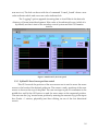
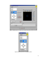
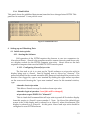
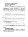
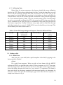
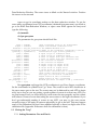
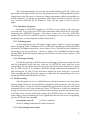
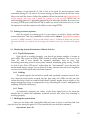
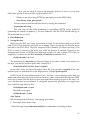
1
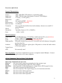
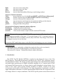
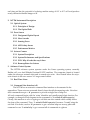
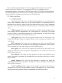
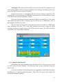
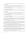
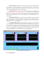
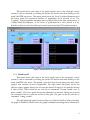
WIYN TIP-TILT MODULE
USER MANUAL
(KPNO SYSTEM)
Version: July 02, 2002
Chuck Claver and Dipankar Maitra
With contributions from
The rest of the world
The Ring Nebula
[send comments on manual to [email protected]]
Overview: Quick Start
General Characteristics:
Arrays:
Image size:
Pixels size:
Read-noise:
DQE:
Dark-current:
Read-out time:
Cosmetics:
Filters:
Saturation:
Gain:
2048 x 4096 EEV CCD; thinned , engineering grade
2048 x 2500 @ 16 bits, plus header, overscan:~10.58 Mbytes
13.5-um ( ~ 0.1125"/pixel )
~4.65 e−
86% peak at 6500Å [find this]
~5 e−/pixel/hr [find this]
2.6 minutes
Fair to good; about half a dozen bad columns; a dozen or so small 1-2
pixel bad areas.
2" x 2"
Typically, linear to 0.1% to 100,000 e~1.983 e−/ADU
WIYN Parameters:
Count Rates:
At UBVRI=20th mag: U: 35; B:330; V: 340; R: 410; I: 225 e-/sec [find this]
FOV:
3.8'x4.2', XIMTOOL Orientation: North- up, East-left
Scale:
0.1125"/pixel at center [determine field distortion]
Image quality:
PSF quite constant across the FOV, but will vary with distance from guide
star less than 10%
Artifacts:
Bright stars will show a ghost plus ~100 pixels in x from the back surface
of the beam splitter.
Typical focus:
ADC:
Not currently used
Data Acquisition: Acquisition commands are given on computer named Navajo -- Analysis
commands are given also on the same computer.
All the Commands That Are Likely To Be Needed
Observing Commands (on wiyn-ccd)
Observe
take one or more exposures prompting for the exposure type
Doobs
a script which takes flats/objects for a list of filters
Mosdither
takes (typically 5) dithered images in a single filter to fill the gaps in array
More
take more exposures just like the last one
Test
take a test exposure. The output image, test, is overwritten each time
Object
take one or more object exposures
Zero
take one or more zero (bias) exposures
Dark
take one or more dark exposures
2
Dflat
Sflat
Focus
Recover
take one or more dome flats
take one or more sky flats
take a focus frame
recover data (if possible) following a crash during readout
Exposure Control Commands
Pause
pause exposure (e.g. clouds) [do not ABORT or STOP from within pause!]
resume
resume a paused exposure [then ABORT or STOP if necessary!]
tchange
increase or decrease the exposure time
Stop
stop an exposure (and sequence of exposures) reading out the detector
Abort
abort an exposure (or sequence) discarding the data
pictitle
change the title of the picture
Quick-look and Taping Commands (driftwood/pecan)
mscdisplay
display an entire mosaic frame
mscexamine general tool for examining images
mscwfits
write mosaic frames to tape in multi-extension FITS format
Caution :Tape your data as you go; DLT-7000 (~250 images/tape) and Exabyte drives (~35
images/tape) are available. Write time: ~75 seconds/image to DLT, ~3 minutes/image to
Exabyte. DDS-4 DAT drive available on Pecan (4m); write time ~40s/image. Please be off
the computer by noon of your last day!
You can buy DLT and Exabyte tapes on the Kitt Peak, but bringing your own is cheaper.
Calibration data:
Take dome flats or, preferably, twilight flats (night sky flats work even better!).
Take dark exposures of similar length to your science exposures.
Take zeroes (i.e., biases) -- Darken the dome for darks and zeroes!
1. Introduction
The WIYN Tip-Tilt Module (WTTM) is attached at the Nasmyth focus of the 3.5m
WIYN telescope. Physically the module is installed at the “WIYN” port, which also houses
the Mini-Mosaic Camera. The design permits rapid change from wide-field CCD imaging
and multi-object spectroscopy to higher resolution imaging over a 5 arcmin field of view
and integral field spectroscopy as science objective and atmospheric seeing dictates. As a
result of the active optics system already installed on WIYN, control of the local
environment and location of the telescope, the image degradation is primarily a result of
upper atmospheric turbulence of which measurements indicate that for an aperture of this
size image motion is a major contributor. The WIYN tip-tilt system corrects this motion in
3
real time and has the potential of reducing median seeing of 0.8" to 0.5" at R and produce
nearly diffraction limited images at H.
2. WTTM Instrument Description
2.1. Optical System
2.1.1. Principles of Design
2.1.2. The Optical Path
2.2. Error Sensor
2.2.1. Design and Optical layout
2.2.2. How it works
2.2.3. Sensing Focus
2.2.4. APD Safety Issues
2.2.5. Performance Metrics
2.3. Science Camera
2.3.1. System Description
2.3.2. System Performance and Specifications
2.3.3. FOV: Why it looks the way it does
2.3.4. Beam-splitters for Science
3. Software Control System
The WTTM software system operates under the Linux operating system, currently
Redhat v6.2 on a dual 500mhz Pentium III CPU machine. The computer chassis is located
under the telescope azimuth skirt and is named wiyn-wttm. Also located below the wiynwttm chassis is the error sensor X-Y stage control chasis.
3.1. Real Time Linux
3.2. Command Line Interface (cli)
The WTTM has an extensive command line interface as documented in the
appendices. These notes are extracted directly from the self-documenting code. Note that
most commands accept a ‘-h’ parameter to provide a single line of help text.
All such commands begin with the ‘wttm’ identifier and usually match their function. For
example, to change the task frequencies the command is ‘% wttmSetTaskFrequencies’.
Clearly, this amounts to a lot of typing so soft links are also created which usually follow
the form of the command. Thus, ‘% wttmSetTaskFrequencies’ becomes ‘% wstf’ using the
soft link. If in doubt, use the ‘-h’ parameter to get a one-line help text on any particular
command or use ‘% wttm help’ to get a screen full of commands at a glance.
4
The cli commands are issued by the observer logged in the computer “wiyn-wttm”
from the terminal of “Almond”. For a greater detail on the cli commands (from a
programmers point of view) refer to “WTTM Users Guide” by P.N.Daly (this should be in
the WIYN Control Room). However all the working of WTTM can also be controlled with
user friendly GUIs developed using Labview as described below.
3.3. Labview Interfaces
3.3.1. WttmControlVI
This panel allows the user to send the main 9 elements to the real-time core.
When these parameter values are set, the button labeled SET PARAMETERS must be
pressed once to send the values to the core (otherwise they are not sent). Remember
that some values can be adjusted whilst the system is in closed-loop mode and some
cannot.
APD Frequency: This value sets the frequency in Hertz for the reading of the 4
APD counters and the computation of the 3 error signals, X, Y and Focus. The system
must be in idle (e.g. paused from pressing the “stop acquisition” on this GUI) in order
for this value to be sent to the real-time Linux core.
APD Update: This value sets the frequency in Hertz that the APD values in the
WttmGetTaskValuesVI panel are updated (more on the consequences relating to this
value later).
DIO Frequency: This value sets the frequency in Hertz that the DIO task
updates the position of the tip-tilt mirror via the Physique-Instrumente control chassis.
This is normally set to the same frequency as the APD Frequency.
DIO Update: This value sets the frequency in Hertz that the DIO values in the
WttmGetTaskValuesVI panel are updated. Typically this is set to the same value as the
APD Update frequency.
Focus Interval: This value sets the interval in Seconds over which the focus
signal is averaged to determine the incremental focus corrections once the focus control
loop is locked.
Guider Interval: This value sets the interval in Seconds over which the
commanded tip-tilt mirror position is averaged in order to determine incremental X
and Y guider corrections.
X and Y milligain: These values set the relative conversion factor between
computed X and Y errors and the additive offset in volts applied to the current mirror
tip-tilt position that generates the next commanded tip-tilt mirror position.
5
Z milligain: This value sets the relative conversion between the computed focus
error and the additive offset in microns applied to the telescope secondary position by
way of the WIYN router to the SecTilt client
is a debugging aid and returns nothing of interest to the
average user. SAVE PARAMETERS and RESTORE PARAMETERS save and recall these 9 items
to the file /home/wttm/development/.wttmrc.
REPORT PARAMETERS
The START ACQUISITION and STOP ACQUISITION buttons are analogous to the pause
and resume functions in the cli. Indeed, you can still use the ‘% wcli pause’ and ‘%
wcli resume’ should you so wish.
The EXIT button in this panel is the main button that sets wttmExit to TRUE and,
thus, terminates all other GUIs. Note that terminate here means ‘stops the GUIs
running’ and does not imply ‘removes the GUIs from the screen’. The GUIs should be
removed by the ‘% wlv stop’ command.
Figure 1: wttmControlVI Panel
3.3.2. WttmGetTaskValuesVI
This panel is the main system monitor and shows the X, Y and Z errors as well
as APD counts for each channel. The following items can be identified (from the
bottom up):
LOGGING?
If checked, all incoming values are appended to taskVI.dat in the data
sub-directory of /home/wttm/development. These files can grow quite large and
should be expunged regularly.
6
DIO COUNT
is the number of times the DIO task has been through its
programming loop.
DIO HW ERROR is
a flag to indicate a DIO hardware violation detected by the realtime core. A zero value indicates no error, a non-zero value is undesireable.
is the typical time take to access DIO hardware from the real-time
core expressed in microseconds.
DIO HW TIME
is the typical time take to complete 1 complete programming loop
(for the DIO task) in the real-time core.
DIO HW TIME
APD COUNT
is the number of times the APD task has been through its
programming loop.
is a flag to indicate a APD hardware violation detected by the
real-time core. A zero value indicates no error, a non-zero value is undesireable.
APD HW ERROR
is the typical time take to access APD hardware from the real-time
core expressed in microseconds.
APD HW TIME
is the typical time take to complete 1 complete programming loop
(for the APD task) in the real-time core.
APD HW TIME
is a graphical representation of the APD counts as a snapshot taken
every APD update rate in Hertz. The 4 APDs are colour coded (0=yellow,
1=green,2=pink,3=purple) and explicit values are also shown in the color-keyed
indicator boxes at the lower right of the graph.
APD COUNTS
X is
the main graphical representation of X errors. The average error is shown in
the upper panel and the variance in the lower panel. The variance is 0.0 (and hence
undefined) when the number of available data points is <2. Data displayed in this
graph can be changed using the ring buffer widget called XYZ Graph.
Y is
the main graphical representation of Y errors. The average error is shown in
the upper panel and the variance in the lower panel. The variance is 0.0 (and hence
undefined) when the number of available data points is <2. Data displayed in this
graph can be changed using the ring buffer widget called XYZ Graph.
Z is
the main graphical representation of Z errors. The average error is shown in
the upper panel and the variance in the lower panel. The variance is 0.0 (and hence
undefined) when the number of available data points is <2. Data displayed in this
graph can be changed using the ring buffer widget called XYZ Graph.
XYZ GRAPH controls what is displayed in the X, Y and Z graphs above. There
are 4 options:
7
Raw APD Errors are snapshot values at the cadence of the task update rate.
For example, if the APD update rate is 20 Hz and this option is selected then
snapshot (raw) values are placed on the buffer by the real-time core every 1/20 s and
these values are displayed in the X, Y and Z graphs.
Raw DIO Errors are snapshot values at the cadence of the task update rate
[looks same as above !!! which one is correct ????]. For example, if the DIO update
rate is 10 Hz and this option is selected then snapshot (raw) values are placed on the
buffer by the real-time core every 1/10 s and these values are displayed in the X, Y
and Z graphs.
Accumulated APD Errors are average data at the cadence of the task update
rate. For example, if the APD task frequency is 1000 Hz and the APD update rate is
20 Hz then 1000 / 20 = 50 data points are averaged and the result (and variance)
displayed via the X, Y and Z graphs.
Accumulated DIO Errors are average data at the cadence of the task update
rate. For example, if the DIO task frequency is 500 Hz and the DIO update rate is 25
Hz then 500/25 = 20 data points are averaged and the result (and variance) displayed
via the X, Y and Z graphs. It gets more complicated than that, however, if the DIO
task is not running at the same frequency as the APD task as the DIO task can
accumulate APD values—check the source code for an explanation!
Figure 2: wttmGetTaskValuesVI Panel
3.3.3. WttmGuiderVI
8
This panel shows the value of the guide signals sent to the telescope control
system. It can be restarted by clicking the (local) exit button and then clicking on the
usual LabVIEW run arrow. The upper panels show the X and Y guide adjustments and
the lower panel the associated variance (if applicable) all in seconds of arc. The
‘Logging?’ options appends incoming data to guiderVI.dat in the data sub-directory of
/home/wttm/development. If the value of guideInterval is zero (which it is by
default) no data is sent to the telescope control system and this GUI remains inactive.
Figure 3: wttmGuiderVI, the guider panel
3.3.4. WttmFocusVI
This panel shows the value of the focus signal sent to the secondary control
system. It can be restarted by clicking the (local) exit button and then clicking on the
usual LabVIEW run arrow. The panels on the left show the incoming raw data value
(upper) and variance (lower) if applicable. The right hand side panel shows the
effective target (upper) taking into account the desired Z target (if set) and the desired
Z offset (if set). These values are set with the cli commands ‘% wszt -t<val>’ and ‘%
wszo -o<val>’. The lower panel shows the adjustment in microns taking into account
the conversion factor to microns and the Z-axis gain. The gain can be set with the cli
command ‘% wsg _z<val>’.
The right hand side panel is activated by use of the lock facility. When unlocked,
the graph is disabled. When locked, the graph is enabled (assuming the focusInterval is
9
non-zero too). The lock can be set with the cli command ‘% wszl _l<val>’ where a zero
value indicates unlock and a non-zero value indicates lock.
The ‘Logging?’ options appends incoming data to focusVI.dat in the data subdirectory of /home/wttm/development. If the value of focusInterval is zero (which it is
by default) no data is sent to the secondary control system and this GUI remains
inactive.
Figure 4: wttmFocusVI, the focus panel
3.3.5. XyManVI: Error Sensor position control
This GUI controls the position of the error sensor ans is used to move the errors
sensor to the location f the desired guide star. The current x and y positions of the error
sensor is shown at the top of the panel. The user can input a pair of coordinates in the
middle box and hit the GO button to send the error sensor at the requested position.
The user can also ‘jog’ around some position by entering the amount to jog in the input
box (2units = 1 micron, physically) and then clicking on one of the four directional
arrows.
10
Figure 5: xyManVI panel, as it comes up. It comtrols the position of the error sensor.
Figure 6: xyManVI panel after resizing the window.
11
3.3.6. WttmPublish
This panel shows the published data stream items that have changed since WTTM. This
panel can be restarted ‘% wttm publish restart’.
Figure 7: wttmPublish Panel
4. Setting-up and Obtaining Data
4.1. Initial start-up tasks
4.1.1. Starting the Software
Full operation of the WTTM requires the observer to use two computers viz.
Almond and Navajo. Almond is the computer used for remote observing and serves only
as a display console for the WTTM computer wiyn-wttm. Navajo serves as the data
acquisition computer that runs the HARCON CCD control system.
4.1.1.1. Configuring Almond/wiyn-wttm
The first task to do is to start up the Tip-tilt software on wiyn-wttm with its
display being sent to Almond. Start by logging onto to Almond as “observer”. The
password should be the normal mountain user password and should be posted on the
monitor. Once logged in, open a new terminal by clicking the right mouse anywhere
on the screen and choosing the “open new terminal” menu. In this terminal window,
type
almond> xhost wiyn-wttm
This allows Almond to accept X-windows from wiyn-wttm.
almond> rlogin wiyn-wttm –l root [this will be changed]
wiyn-wttm> export DISPLAY=”Almond:1”
This is a bash shell command that tell wiyn-wttm top send all X-window display
from this session to Almond’s screen number 1. Note: On Almond the default login
screen is the 24 bit display and is referred to as Almond:1, where the alternate 8 bit
display is referred to as Almond:0. At this point Almond and wiyn-wttm should be
configured to start WTTM software.
12
4.1.1.2. Starting WTTM software on wiyn-wttm
In the wiyn-wttm terminal window type
wiyn-wttm> wlv start
This will start the WTTM Labview software which enables the user to control
the operation of the tip-tilt module. A few messages will appear on the terminal,
followed by opening of five GUIs with titles WttmPublish, WttmControlVI,
WttmGetTaskValuesVI, WttmGuiderVI and WttmFocusVI. The WttmControlVI
window is the most important of all these because it is through this GUI that user feeds
all the inputs to control the WTTM. The rest are mainly for visualizing the outputs and
checking for erroneous behaviour (if any). The user may want to minimize the
WttmPublish as it is the least needed (in fact not at all if things are going fine!). The
other windows may also be moved and resized to use the monitor screen efficiently.
Now type
wiyn-wttm>xyManVI &
to start the GUI to position the error sensor. Fig.5 shows the window that comes
up. However the user may resize it to resemble Fig.6 without any loss in efficiency.
This completes the initial startup process for the WTTM and now the observer may
proceed to setup Navajo, the computer used for data collection.
Configuring Navajo
The data acquisition takes place in Navajo. Login as “wiyn_ccd”. The password
should be posted on the monitor. Along with various ARCON windows, an IRAF Data
Acquisition Window and another IRAF Data Reduction Window opens up. An
Ximtool window also opens up which shows the most recently acquired image. Right
click and (Re)start ARCON if it is not already running.
4.1.2. Initial Configuration
In the WttmControlVI set the APD/DIO frequencies and APD/DIO update
rates as shown in Fig.1. But keep the X,Y and Z milligains to zero, to keep the loop
open. Hit the Set Parameters button and then Start Acquisition. The user will notice
that the APD counter in wttmGetTaskValuesVI becomes alive. However the counts in
all 4 APDs is zero because during the startup, the power in the APDs is off by default
(to increase the longevity of the APDs). To turn the power in the APDs on, issue the
command:
wiyn-wttm>wttm_pwr apd on .
Similarly wiyn-wttm>wttm_pwr apd off turns power in the APDs. When the
power in the APDs is turned on, a brief surge of counts from each APD is seen[why ?].
After this brief surge, the counts will come down to ~2 or 3 counts for each APD. This
ensures that the system is working properly.
13
4.1.3. Calibration Data
Before/after the science exposures, the observer should take some calibration
data for the CCD. This invloves taking dome/sky flats. To take the dome flats you will
have to tell the observing assistant first that you intend to do so. Once you get his
green signal you should right click anywhere on the desktop on Navajo and select the
Domeflat menu. Once the GUI comes up[need a screenshot of that], turn the high lamp
on at your selected intensity (Table 1 may be a useful starting point). Once the lamps
are on you can actually see them in the TV in the control room. You may use either the
observe command or the dflat/sflat and zero command to take dome/sky-flats and the
bias frames respectively. Usually 5-10 biases every night, and five dome flats through
each filter (aiming for a count of ~20,000 ADUs in each) should be good enough. This
should flatten your data to better than 1%.
Table 1: Dome-Flat Lamp Settings and Exposure Times for different Filters
FILTER
HIGH LAMP
INTENSITY
EXPOSURE (s)
Approximate Count
(ADUs)
Harris V
2000
4
20,300
Harris R
1500
3
20,600
Harris I
1000
5
20,000
Gunn r
1800
4
20,800
Gunn I
1100
5
20,500
Gunn z
1200
4
22,300
1.1. Getting on Sky
1.1.1. Initial Focus
After you get to your field, take a quick snapshot of the field, by typing in the
data acquisition window
cl> test
Do a quick focus sequence. When you take a focus frame with the ARCON
software at WIYN, you typically take a short (3-10 sec) exposure of a 11-12th mag star,
clock the charge down 30 rows, decrease the focus value, take another exposure, clock
down the charge, decrease the focus, etc., for a series of 7-9 exposures. The frame is
then read down, the the image examined with mscexam/mscfocus to determine the
best focus value. Note that the double-space gap occurs after the first exposure. A
sample run is shown in Fig. 6.
14
1.1.2. Acquiring your field [details of “observe” command ? already there in
MINIMO manual]
Figure 8: A focus run centered at 4800 and step size -20
1.2. Selecting a guide star
Select a fairly bright star (mv between 10-15)near you object of interest. Try to
make sure that the star you chose is not variable [why?]. Type mscexamine on the IRAF
15
Data Reduction Window. The cursor turns to blink on the Ximtool window. Position
the cursor on the star and
type a to get its coordinate written on the data reduction window. To get the
error sensor coordinates from CCD coordinates (obtained from mscexam), one needs to
go to the IRAF Data Reduction Window, or open a new IRAF xgterm on Navajo and
type the following:
cl> immatch
cl> lpar geoxytran
The parameters for geoxytran should look like
input
output
database
transforms
(geometry
(xref
(yref
(xmag
(ymag
(xrotation
(yrotation
(xout
(yout
(xshift
(yshift
(xcolumn
(ycolumn
(calctype
(xformat
(yformat
(min_sigdigit
(mode
=
=
=
=
=
=
=
=
=
=
=
=
=
=
=
=
=
=
=
=
=
=
"STDIN"
Input coordinate files to be transformed
"STDOUT"
Output transformed coordinate files
"ES_CCD_trans.fit" The GEOMAP database file
"ES_CCD_trans.dat" Names of the coordinate transforms in the da
"geometric")
Transformation type (linear,geometric)
INDEF)
X input origin in reference units
INDEF)
Y input origin in reference units
INDEF)
X scale in output units per reference unit
INDEF)
Y scale in output units per reference unit
INDEF)
X axis rotation in degrees
INDEF)
Y axis rotation in degrees
INDEF)
X output origin in output units
INDEF)
Y output origin in output units
INDEF)
X origin shift in output units
INDEF)
Y origin shift in output units
1)
Input column containing the x coordinate
2)
Input column containing the y coordinate
"real")
Data type for evaluation coordinates
"")
Output format of the x coordinate
"")
Output format of the y coordinate
7)
Minimum precision of output x and y coordinates
"ql")
Run geoxytran and input the CCD coordinates to get Error Sensor coordinates.
Set the coordinates in xyManVI and “go” there. The counts in each APD should rise as
the error sensor gets to the star. The counts may not be balanced in each APD to begin
with, but as long as you are getting a good number of counts in at least one APD, you
are fine because once you close the loop it will center the star properly and the counts
will balance. However even after taking the error sensor to the right coordinates if you
don’t get substantial number of counts in any APD, you may jog the error sensor
around in steps of 100 units (50 microns physically) to get to the star. This may happen
rarely if the calibration file hasn’t been updated recently or there is a slight error in the
calibration file (Appendix B discusses how the calibration is done).
1.3. Closing the “loop”
1.3.1. Setting Parameters: Dos and Don’ts
16
The control parameters are set from the wttmControlVI panel. Fig.1 shows the
panel with some typical values used for the parameters used. All the parameters can be
changed any time (however you better not change parameters while in the middle of a
science exposure). To change any parameter, first change its value in the box, then hit
Stop Acquisition followed by Set Parameters. Then you are ready to Start Acquisition
again.
1.3.2. Selecting a frequency
Generally an APD/DIO frequency of 200 Hz is a good point to start once you
are at the star. Try to bring the APD counts somewhere between 20-40 for each APD.
Increasing the APD/DIO frequency will reduce counts and vice-versa. APD/DIO
update rate of 10-20 Hz should be good for most purposes (our eyes hardly notices
anything faster, so increasing this wouldn’t help much !).
1.3.3. Selecting a gain
At low frequencies you will need a larger value of gain to correct for image
motion. Keeping X and Y milligains to 50 for APD/DIO frequency around 50-200 HZ is
reasonable. For higher frequencies a lower value of 10 or 5 should be good. Similarly if
the seeing is not very good (say ~1 arcsec or higher), the Z milligain should be high
(around 1000). When the seeing is quite good (0.6 arcsec or lower), even a value of ~500
should be good.
1.3.4. Telescope Guiding
Usually the guiding in WIYN is done by choosing a guide star nearby the field
and the autoguider tracks the star. However for WTTM we don’t need any extra
autoguiding, our star chosen above for doing the tip-tilt correction itself acts as a guide
star. A Guider Interval of 5 seconds is should be enough under most circumstances. So
after closing the X,Y and Z loops and before setting the focus interval to a non-zero
value one must ask the telesccope operator to make sure the autoguiding is off. Once
operating WTTM itself will take care of that.
1.4. Final Focussing
Once the gains are set ( i.e. feedback loop is closed for motion on the focal plane
and any image motion on the focal plane is annulled) for the guide star, and the star is
reasonably close to focus, the observer should take another focus sequence with small
increments (10 or even 5 step increment). Since WTTM tries to extract the maximum
seeing, it is crucial to focus it very accurately before starting. Request the operator to go
to the best focus, wait for about half-a-minute (for WTTM to know its reference focus,
from where it starts calculating the focus signals)and then lock the focus (for updating
only by WTTM) by the command
wiyn-wttm> wszl –l1
[1 locks, 0 unlocks]
Set the Z milligain and then hit ‘Start acquisition’.
1.4.1. Closed Loop Focus Control
17
Setting a focus interval of ~30s is seen to be good for most purposes under
reasonable seeing (0.7-1.0 arcsec). For worse seeing you may decrease it and vice-versa.
How-ever until the focus is locked the updates will not be carried out [I am not sure it
works exactly this way, but I think so, correct if I am wrong]. WIYN has an
autofocussing option too, generally operated by the telescope operator. But when you
are using WTTM you would like WTTM to make any focus corrections for you, so ask
the operator to turn the autofocus off while you are using WTTM.
1.5. Starting a science exposure
Once the tip-tilt is working good, it is now time to go back to Navajo and take
science exposures. The only command you really need is observe. [give full description
or refer to MIMO manual ? when to take dflats, zeros ? if different filters are used for
the same field do you unlock the focussing, do another focus seq. and then lock again
?]
1.6. Monitoring System Performance: What to look for
1.6.1. Tip-tilt Performance
If the tip-tilt is working properly, you should get decent number of counts in
each APDs. The counts in all the APDs should be nearly balanced. The errors for all
three X,Y and Z axes should be scattered randomly, close to zero. Any
increasing/decreasing trend in time points towards something going wrong. Usually
we look at the “Raw APD errors” rather than the “Accumulated” errors because the
accumulated errors average over an interval of time, whereas raw errors are snapshots
of errors in the APDs taken after fixed time interval.
1.6.2. Guiding
The guide signals also should be small and randomly scattered around zero.
Any observed trend points towards the fact that either the APDs lost the star (the
counts should go down in wttmGetTaskValuesVI panel), maybe due to clouds, or the
image motion is too large to compensate for (try increasing the X and Y milligains and
reducing APD/DIO frequency).
1.6.3. Focus
As intuitively expected, the values of the focus signal sent to the telescope
should also be small and randomly scattered around zero when the focussing is
working properly.
1.7. Shutting the system down
Once you are done with a particular field and want to move to another field, first
open the loop by setting the gains to 0. Then unlock the focus with the command
wiyn-wttm> wszl –l0
18
Now you are ready to request the telescope operator to move to your next
field. After getting to the next field, repeat from Sec. 4.2.1.
When you are done using WTTM for the night, power the APDs off by
wiyn-wttm> wttm_pwr apd off
You may want to shut the software down by issuing the command
wiyn-wttm> wlv stop
This will close all the GUIs pertaining to ccontrolling WTTM except xyManVI
(remember we started it separately ?). To close xyManVI, click the STOP buttom, then go to
File menu and choose ‘Quit’.
2. Data Reduction
3. Saving the data
Right now the DAT tape drive is mounted on Sand. So the observer has to ftp all his
data to Sand. Both Exabytes and DATs are available. These are mta for the Exabyte drive,
and mtb is the DAT drive. The DAT supports DDS-4 densities (20 Gbytes per tape). The
DAT on sand is internal to the tower box while the Exabyte is external. Because of the
multiextension format of WTTM data (although actually it is only a single CCD with one
amplifier), you must use the IRAF mscwfits and mscrfits commands. Do a
cl>allocate mtb from Sand.
The parameters for mscwfits are shown in Figure #. In order to check to see what is on
the tape, you can list the titles quite easily. Simply do a
cl>mscrfits mtb 1-999 list+ short+ original+
to see what's there. To direct this output into a file, you can add a > tapelist to the end,
and then you can print that list on the lineprinter by a simple lprint tapelist.
NOTE: If you do write additional files to an ``old tape'' (one containing useful data but
which had previously been removed from the drive), make certain that the software (IRAF
and Unix) is aware that the tape has been rewound before starting to write to the tape----or
your old data may be overwritten! To safeguard against this possibility we suggest that
you ALWAYS swap tapes by first:
cl>deallocate mtb (or mta)
Physically swap tapes
cl>allocate mtb (or mta)
Safe Taping
We recommend the following ``safe taping'' procedures.
1. Each night write data to tape.
2. Read the tape using cl>mscrfits mtb list+ to substantiate everything is there.
19
3. Deallocate the drive, remove the tape, and stick it under your pillow.
4. Make a second copy of your tape. (This tape could be an accumulative copy of the
data throughout your run.) Check this tape with mscrfits!
5. Only now delete the data from disk if necessary.
Save-the-Bits!
All data taken at WIYN (and the other Kitt Peak telescopes) are automatically saved to
tape. Extracting a night's worth of data from these tapes is laborious and labor- intensive,
and we strongly emphasize the need for the ``safe taping'' procedures above. But if you
ever do need to recover a night's worth of data, take heart! You can send email to
[email protected] .
Writing CDROMs
You can also take your data home on CDs, but be forewarned that you will need about
4-5 CDs per night of observing. They hold only about 650 Mbytes of data. Instructions for
writing CDROMs can be found at: http://claret.kpno.noao.edu/wiyn/cd write.html . Note
that you should use the CD writer on sand rather than pearl; otherwise the instructions
should work. You can then check the CDs by placing them in the CD reader on sand and
displaying from the directory /mnt/cdrom.
4. Issues about Astrometry and Photometry
Appendix A; Recognizing when things go wrong and what to do
Appendix B: Calibrating the CCD – Error Sensor Coordinates
The CCD- Error Sensor Coordinates are calibrated by uniformly illuminating (the lights
for dome flats are good) an array of 5 x 5 pinholes, each of 5u dia., placed at the Nasmyth
focus of WIYN. The CCD position of each pinhole was noted by briefly exposing the chip.
Then their corresponding positions on the Error Sensor were found by putting the tip-tilt
correction on and jogging around (see the xyManVI GUI) till the x and y tilts were
effectively nulled out. This procedure shouldn’t be required unless there is any physical
disturbance to the WTTM unit. However it might be a good to check this calibration from
time to time in order to make sure everything is fine. As a starting point for a calibration
run, use the earlier input coordinate file (es_trans.dat) to assess the Error Sensor coordinate
for a given CCD coordinate. Remember to open the loop (set X and Y milligain to zero)
before moving from one pinhole to another.
As the keen observer has surely noted ,the CCD chip has 2048 x 2500 pixels whereas the
XY Error Sensor scale ranges from 0 to 80,000 in either directions (as seen in the xyManVI
window). Actually the transformation from CCD coordinates to Error Sensor coordinates is
not just linear but has higher order terms it. However this calibration is already done
beforehand and the user doesn’t have to worry about it. However the user must supply the
error sensor coordinates of the star he/she wishes to use as a guide star.
20
The most recent data file for calibration file is es_trans.dat [where these files are? there
should be a common repository for these files]. The transformation from CCD to Error
Sensor coordinates is done by the “geomap” task in the IRAF “immatch” package. An lpar
on geomap should look like the following:
input
database
xmin
xmax
ymin
ymax
(transforms
(results
(fitgeometry
(function
(xxorder
(xyorder
(xxterms
(yxorder
(yyorder
(yxterms
(reject
(calctype
(verbose
(interactive
(graphics
(cursor
(mode
=
=
=
=
=
=
=
=
=
=
=
=
=
=
=
=
=
=
=
=
=
=
=
"es_trans.dat"
"es_trans.fit"
INDEF
INDEF
INDEF
INDEF
"es_trans")
"")
"general")
"polynomial")
4)
4)
"half")
4)
4)
"half")
INDEF)
"real")
yes)
yes)
"stdgraph")
"")
"ql")
The input coordinate files
The output database file
Minimum x reference coordinate value
Maximum x reference coordinate value
Minimum y reference coordinate value
Maximum y reference coordinate value
The output transform records names
The optional results summary files
Fitting geometry
Surface type
Order of x fit in x
Order of x fit in y
X fit cross terms type
Order of y fit in x
Order of y fit in y
Y fit cross terms type
Rejection limit in sigma units
Computation type
Print messages about progress of task ?
Fit transformation interactively ?
Default graphics device
Graphics cursor
Then the “geoxy” task could be used to find the Error Sensor coordinates for a given
pair of CCD coordinates.
21