Download Report

Implementation of a Pragmatic Translation
from Haskell into Isabelle/HOL
Patrick Bahr
December 18, 2008
Abstract
Among other things the functional programming paradigm – in its pure form
– offers the advantage of referential transparency. This facilitates reasoning over
programs considerably. Haskell is one of the rare purely functional programming
languages that is also of practical relevance. Yet, a comparable success for the
verification of Haskell programs has not been achieved, so far. Unfortunately, Haskell
lacks a decent theorem prover. On the other hand, the theorem prover Isabelle allows
specifying functional programs in its logic HOL. We present an implementation –
written in Haskell – which enables to translate Haskell programs into Isabelle/HOL
theories. This approach is pragmatic, since its focus is to produce theories that are
easily readable and minimise the effort to construct proofs. To this end we had to
sacrifice soundness and completeness of the translation. Nevertheless, in practice
this kind of translation has proven to be adequate and powerful. We also show
some of the techniques that we have used for the implementation including meta
programming and generic programming.
1 Introduction
In general an automated translation from programming languages into the language of a
theorem prover may provide useful support for the verification of programs. It is widely
established that functional languages, due to their declarative style and comparatively
simple semantics, facilitate the effort of proving properties of programs written in them
(cf. [22, 21]). This is particularly true for the purely functional programming language
Haskell. Due to its purely functional semantics it allows equational reasoning which
simplifies proofs about programs considerably. On the other hand, as a result of its
growing richness in features, including a sophisticated strong type system, it has found
its way into a large number of practical applications (cf. [8, Part IV]). This also stems
from the fact that the language still allows to write imperative code, which is nicely
separated from its pure semantics using the concept of a monad [16] in conjunction
with the language’s comprehensive type system. The generic theorem prover Isabelle
[18] provides a modular collection of tools which enable reasoning about a variety of
1
different logics. In particular we are interested in its logic HOL, a classical higher-order
logic based on the simply typed lambda calculus. It allows to specify functional programs
and to prove properties about them quite efficiently.
Our aim is to combine these two systems by providing an automated translation from
Haskell into Isabelle/HOL. The focus of our endeavour is set on producing Isabelle/HOL
theories which are still close to the original formulation in Haskell and which, therefore,
alleviate the effort of constructing proofs. This is the reason for choosing Isabelle/HOL
as the target languages rather than a richer logic like Isabelle/HOLCF. Isabelle/HOLCF
[17] is a conservative extension of Isabelle/HOL by Scott’s Logic of Computable Functions. This logic is well suited to describe Haskell’s non-strict semantics as well as partial
functions. We do not attempt to achieve similar results within Isabelle/HOL.
In fact the choice of the target logic Isabelle/HOL causes a number of difficulties
when trying to formalise a Haskell program. This includes Isabelle/HOL’s weaker type
system as well as it’s inability to formalise partial functions. The latter is indeed a
problem for Haskell’s non-strict semantics. Therefore, our implementation will not be
able to translate programs correctly which depend on Haskell’s non-strict semantics.
The problem that we are facing, regarding Isabelle/HOL’s type system, is its inability
to express type constructor classes. This has significant consequences, as this prevents
a proper translation of monadic Haskell programs.
Nevertheless, the implementation we are presenting here is able to translate most of
the Haskell 98 language [12]. This includes
• case, if-then-else, and let expressions;
• list comprehensions;
• where bindings and guards;
• mutually recursive functions and data type definitions;
• simple pattern bindings;
• definitions and instantiations of type classes; and
• monomorphic uses of monads including the do notation.
On the other hand the translation is not able to treat
• constructor type classes and consequently polymorphic uses of monads;
• non-simple pattern bindings; and
• irrefutable patterns.
In other words this translation is not complete. Furthermore, due to the semantics
of Isabelle/HOL, Haskell programs that depend on the non-strict semantics of Haskell
cannot be translated correctly. This leads to an translation which is in general unsound.
2
Despite these flaws this translation has a considerable advantage: As the resulting
Isabelle/HOL theories are very close to the original Haskell code, proofs are much less
complicated compared for example to a translation into Isabelle/HOLCF. Moreover, this
approach has proven to be adequate in practice provided a non-strict semantics is not
crucial [3].
Our implementation is based on the work by Florian Haftmann and Tobias Rittweiler.
Our contribution to this consists of a number of extensions which either extend the subset
of Haskell that can be treated or which correct parts of the translation. Section 2 briefly
describes the implementation our work is based on. Section 3 presents our extensions
to the previous work. In Sections 4 and 5 some of the techniques that we used for
the implementation are described. Additionally, we refer to related work in Section 6.
Section 7 concludes this report.
2 Previous Work
Fortunately, we did not have to start from scratch to implement our desired translation.
We took the opportunity to base our implementation on the work by Tobias Rittweiler
and Florian Haftmann. Their implementation is able to translate a substantial sublanguage of Haskell into Isabelle/HOL. In the following we briefly describe the design of
their implementation. This is particularly important since we will embed our contributions into this framework to get the desired result.
2.1 The Overall Design
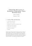
The translation into Isabelle/HOL is performed in six steps:
• Parsing,
• Preprocessing,
• Analysis,
• Conversion,
• Adaptation, and
• Printing.
The bird’s eye view of the translation process is depicted in Figure 1. After the Haskell
source code is parsed into a set of abstract syntax trees, the translation proceeds to the
preprocessing phase during which the syntax trees are transformed into semantically
equivalent but “simpler” ones. This is done to simplify the next steps. Afterwards the
syntax trees are analysed to extract some information about the environment the Haskell
program defines, i.e., information about identifiers (functions, types etc.) that are defined in the program. This global information is needed in the next phase in which the
actual translation is performed. During the conversion step the preprocessed Haskell
3
Haskell modules
1. Parsing
Haskell syntax trees
2. Preprocessing
Haskell syntax trees
(simplified)
3. Analysis
4. Conversion
Isabelle syntax trees
(intermediate)
Context
Information
5. Adaptation
Isabelle syntax trees
6. Printing
Isabelle theories
Figure 1: The overall design of the translation process.
syntax trees are translated into Isabelle/HOL syntax trees. In the subsequent adaptation step references to the built-in Haskell library are changed such that corresponding
definitions of the Isabelle/HOL library are used instead. Eventually the resulting syntax
trees are printed to Isabelle theory files. In the following sections we detail each of the
steps of the translation.
2.2 Parsing
The parsing is delegated to the library haskell-src-exts that is able to parse not only
Haskell code as defined by the Haskell 98 Report [12] but also most of the extensions
to the language as provided by the Haskell implementations Hugs and GHC. Usually a
Haskell module depends on a number of other Haskell modules that are declared as such
via an import statement. These modules are tried to be located on the file system and
parsed as well. In particular this process respects the hierarchical module namespace
4
extension [14] which is not part of the Haskell 98 Report. This process is repeated until
all dependencies are resolved.
An important thing to note is that the parser, of course, only verifies the context-free
part of the syntax. That is, context-sensitive syntax restrictions, such as type-correctness
or the fact that identifiers referred to in an expression are defined, are not checked!
Throughout the translation process we assume that the parsed program is syntactically
correct.
2.3 Preprocessing
To simplify the work that has to be done in subsequent steps of the translation, the
Haskell syntax trees obtained from the parser are transformed to semantically equivalent
but in some sense “simpler” ones. This mostly affects syntactic sugar that is not available
in the Isabelle/HOL language:
(1) Guards in function definitions and case expressions are transformed into if-then-else
expressions. That is, a defining equation
fname patterns
| bexp1
| bexp2
= exp1
= exp2
.
.
.
| bexpn
= expn
| otherwise = expn+1
that contains guarded alternatives is transformed into
fname patterns = if bexp1 then exp1
else if bexp2 then exp2
.
.
.
else if bexpn then expn
else expn+1
If no otherwise clause exists, an additional clause
| otherwise = undefined
is assumed. That is, the corresponding translation ends with else undefined.
Similarly, case expressions containing guarded alternatives are transformed.
(2) Local function definitions, i.e., those defined within let expressions and where bindings are transformed into top-level definitions. That is,
let fname patterns1 = exp1
...
fname patternsn = expn
in exp
5
is transformed into
exp[fname/fname 0 ]
plus an additional top-level definition
fname 0 patterns1 = exp1 [fname/fname 0 ]
...
0
fname patternsn = expn [fname/fname 0 ]
where fname 0 is a fresh name and exp[fname/fname 0 ] denotes the expression that
is obtained from exp by replacing all free occurrences of fname by fname 0 . The
generation of fresh names is implemented by a monad that keeps a counter and
produces a fresh name by appending the counter value to the name and increasing the
counter afterwards. The same monad is used at other places in the implementation
where fresh names are needed.
(3) As-patterns are transformed into additional pattern matchings. An occurrence of an
as-pattern, say,
name@pattern
that is then used by an expression, say, exp will be transformed into the irrefutable
pattern name. Compensating for the missing pattern, the expression exp is enclosed
by an additional case expression like this:
case name of
pattern -> exp
Hence, multiple as-patterns will lead to a nesting of case expressions.
(4) Identifiers of predefined library entities are renamed to avoid clashes.
2.4 Analysis
During the translation of the Haskell syntax trees into Isabelle/HOL syntax trees additional global information is needed. This includes:
• The type annotation for a function definition (if present),
• the module where an identifier was defined,
• what kind of entity (type, type class, function, operator etc.) an identifier refers
to, and
• the precedence and associativity an operator is declared to have.
To this end all top-level declarations are examined in order to collect the necessary
information, which is then stored as a map from identifiers to the representations of this
information.
6
2.5 Conversion
During the conversion step the translation of Haskell syntax trees into Isabelle/HOL
syntax trees is performed. This is done by a traversal through the syntax trees using
a monad that provides the context information, that was collected during the traversal
so far, as well as the global context information collected during the analysis step as
described above. Additionally, the monad provides means to generate helpful error
messages by maintaining a trace of the traversal. This design – which also contains
some other technical neatnesses – turned out to be very powerful as it allowed us to
apply changes fairly easily.
Most of the difficulties of the translation were dealt with in earlier steps or will be dealt
with in the adaptation step afterwards. Yet, one non-triviality has to be solved here:
The order in which types and functions are defined in a Haskell module is irrelevant,
whereas in Isabelle/HOL functions and types cannot be used until they are defined.
That is, the sequence in which functions are defined has to be reordered such that a
function is defined before it is used in another definition. Moreover, function definitions
that are defined mutually recursively have to be defined en bloc in Isabelle/HOL. Both
issues are solved by generating a dependency graph and computing its strongly connected
components (SCCs). Each SCC having more that one element corresponds to a mutually
recursive definition and is turned into a single definition. The partial order defined by
the resulting dependency graph (with the SCCs collapsed) is then used to reorder the
definitions.
Now with all difficulties tackled the translation into Isabelle/HOL does not reveal any
surprises:
• Function bindings are translated into the Isabelle/HOL command fun.
• Simple pattern bindings are translated into the Isabelle/HOL command definition .
• Data type declarations are translated into the Isabelle/HOL command datatype.
• Type class declarations are translated into constructive type classes [4] using the
command class.
• Instance declarations are translated into the Isabelle/HOL command instantiation.
Due to the preprocessing, the translation of Haskell expressions and patterns is almost one-to-one. Only a few technical subtleties have to be taken into account such as
associativity and precedence of operators etc.
2.6 Adaptation
During this step identifiers that refer to entities defined in the Haskell library are renamed
such that they refer to the corresponding entity in the Isabelle/HOL library instead. This
also involves producing a prelude Isabelle/HOL theory that defines some entities of the
Haskell library for which there are no direct correspondents in the Isabelle/HOL library.
Each translated Haskell module imports this prelude theory.
7
2.7 Printing
The pretty printing of the generated Isabelle/HOL syntax trees is performed using the
standard pretty printing library [10] embedded in a monad to propagate some context information as well as the environment information that was generated during the analysis
step.
2.8 Issues of the Original Implementation
Beyond the issues of having HOL as the target logic, the implementation as outlined
above had some problems that needed to be addressed. Most of these shortcomings are
due to the fact that Isabelle/HOL does not provide direct correspondents to some of
Haskell’s features:
• Data types with field labels are not translated: Haskell provides a lightweight extension to algebraic data types that allows them to be used as a record structure.
There is no direct correspondent in the Isabelle/HOL language. Our solution is
presented in Section 3.1.
• Closures of local function definitions are not translated. The reason for this is
rather indirect. The translation turns local function definitions (i.e., those within
where and let) into top-level definitions. However, local functions can refer to
variables that are only bound in the context the function is defined in. If this is
the case, additional effort is necessary when transforming those function definitions
into top-level definitions. The original implementation was not able to take care
of this. For more information on this see Section 3.2.
• Constructor type classes are not subsumed by Isabelle/HOL’s approach to constructive type classes. This is particularly unfavourable as this implies that monads – a ubiquitous concept in Haskell which is too important to neglect it – cannot
be translated into Isabelle/HOL directly. A more elaborate discussion on this is
given in Section 3.3.
Some other things were simply not considered but are crucial for our purposes:
• The implementation does not allow to substitute certain Haskell modules (e.g.,
library modules) by hand-written Isabelle theories. Our extension which provides
this functionality is described in Section 3.4.
• Dependencies between types and between functions and types were not taken into
account: Like function definitions also data type definitions have to be given in the
right order, and mutual recursive data types have to be defined en bloc. Moreover,
data types can only be used in a function definition if they were defined beforehand.
Unfortunately, these issues are ignored by the implementation. More information
on this is given in Section 3.5.
8
• The translation of as-patterns is unsound! As-patterns are transformed in the preprocessing step by introducing an additional case expression for each as-pattern
that occurs in a pattern. Unfortunately, this transformation is not equivalence
preserving. The problem is that the matching against the subpatterns that are
named by an as-pattern construct is moved to the additionally introduced case
expressions. Therefore, the refutation of these subpatterns in the transformed program will immediately yield the value ⊥ whereas the refutation of the subpatterns
in the original program yields refutation of the whole pattern. Then an alternative pattern that might have be given will be considered instead. A more detailed
discussion can be found in Section 3.6.
• Similarly, also the translation of guards is unsound! As already mentioned, the
original implementation translated guards by transforming them into cascaded
if-then-else expressions during the preprocessing step. However, the semantics of
failure of a sequence of guarded alternatives is non-local in contrast to the semantics
for if-then-else expressions. That is, if all guards are not satisfied, then the next
pattern match in the context is considered, i.e., the next defining equation for a
function definition or the next case for a case expression. Therefore, the naïve
translation, as it was done by the original implementation, yields an incorrect
result whenever not all cases are exhaustively covered by a sequence of guards.
For more information consult Section 3.7
As indicated we will describe how we dealt with these shortcomings in the next sections.
3 Extending the Implementation
Our goal is it to be able to translate a large sublanguage of Haskell into Isabelle/HOL
and to avoid unsound translations as much as possible. To this end we extended the
implementation described in Section 2. In the following we describe these contributions.
3.1 Data Types with Labelled Fields
Haskell provides a lightweight extension to run-of-the-mill algebraic data types that
allows using them like records. Instead of just listing the argument types of a constructor
when defining an algebraic data type, the programmer can give each element a label
which can be used to refer to it later. Here is an example of how this can look like:
data MyRecord = A { aField1
common1
common2
| B { bField1
bField2
common1
common2
::
::
::
::
::
::
::
9
String ,
Bool ,
Int }
Bool ,
Int ,
Bool ,
Int }
| C Bool Int String
There are two things worth mentioning: Firstly, constructors with unlabelled elements
can be mixed with constructors with labelled elements within the same data type. Secondly, fields of the same type can be shared between constructors within the same data
type as it is the case for the fields common1 and common2 in the example above.
Labelled fields come along with a syntax that allows the programmer to refer to the
field labels when pattern matching against, updating or constructing elements of a data
type:
constr :: MyRecord
constr = A { aField1 = " foo " , common1 = True }
update :: MyRecord -> MyRecord
update x = x { common2 = 1 , common1 = False }
pattern
pattern
pattern
pattern
:: MyRecord
A { common2 =
B { bField2 =
( C _ val _ )
-> Int
val } = val
val } = val
= val
Isabelle/HOL provides support for records and, of course, for algebraic data types.
However, there is no direct correspondent for this unusual mixture of both concepts.
Nevertheless, since this feature is a rather lightweight one, it can be translated easily to
ordinary data types plus additional projection functions for each field. Also the syntactic sugar for pattern matching, updating and constructing as illustrated above can be
removed. The Haskell 98 Report [12, Sections 3.15, 3.17.3] provides details on the necessary transformations to deal with labelled fields. According to these transformations the
above definitions are equivalent to the following definitions that dispense with labelled
fields:
constr :: MyRecord
constr = A " foo " True ⊥
update :: MyRecord -> MyRecord
update x = case x of
A v1 v2 v3
-> A v1 False 1
B v1 v2 v3 v4 -> B v1 v2 False 1
_
-> error " Update error "
pattern
pattern
pattern
pattern
::
(A
(B
(C
MyRecord -> Int
_ _ val )
= val
_ val _ _ ) = val
_ val _ )
= val
Additionally, each labelled field implicitly defines a function that projects to the corresponding field of the data structure. Made explicit these functions would be defined
10
like this:
aField1 :: MyRecord -> String
aField1 ( A x _ _ ) = x
common1 :: MyRecord -> Bool
common1 ( B _ _ x _ ) = x
common1 ( A _ x _ ) = x
.
.
.
Therefore, the obvious way of treating labelled fields in our translation seems to be an
additional program transformation in the preprocessing phase (cf. Section 2.3). But to
be able to do the necessary transformations for the pattern matching, constructing and
updating syntax we need information about the data type that is involved. Information
of this kind is not collected until the analysis step (cf. Section 2.4) and is, therefore, not
accessible during the preprocessing.
Hence, the translation of the labelled fields syntax into Isabelle/HOL is done directly
during the conversion step (cf. Section 2.5) – i.e., without transforming it in the preprocessing step beforehand. Yet, we still need to collect the necessary information about
data types introducing labelled fields. Fortunately, most of the infrastructure to do this
was already implemented as part of the analysis step (this was the reason for deferring
the treatment of the labelled fields syntax in the first place). In particular, it provides a
means to collect information about so-called constants, i.e., defined functions and operators, and makes it available for later use by creating a look-up table. We just added new
cases for field labels and data constructors. Storing for each field label in which data
constructors it occurs and for each data constructor which field labels it defines turned
out to be sufficient.
The resulting translation is almost the one that would be obtained by first applying
the transformation to remove the labelled fields syntax as described in the Haskell 98
Report and then performing the usual straightforward translation into Isabelle/HOL.
Concerning the update syntax of labelled fields we did not stick to the translation given
by the Haskell 98 Report. The reason is that it would bloat up the expression considerably, which is unfavourable for readability but also makes proofs working on such
expressions unwieldy. This “in-line” approach enlarges the expression depending on the
number of fields and how they are shared between different constructors, as it can be
seen in the example above. That is why we used a different transformation equivalent to
this following the treatment of field labels used as projection functions: For each labelled
field an update function is generated. For example for the field common1 of the data type
MyRecord the following Haskell function would be generated:
update_common1 :: Bool -> MyRecord -> MyRecord
update_common1 x ( B f1 f2 _ f4 ) = B f1 f2 x f4
update_common1 x ( A f1 _ f3 ) = ( A f1 x f3 )
This function update_common1 takes a value for the field common1 and provides a
function that takes an element of type MyRecord and returns this element with the new
11
value for the field common1. If more than one field should be updated the corresponding
update functions are combined by function composition. For the function update in our
example the transformation would yield
update :: MyRecord -> MyRecord
update x = ( update_common1 False . update_common2 1) x
As mentioned before, the reason for this discussion on transforming Haskell programs
to get rid of labelled fields is to illustrate the idea of the final translation. Due to
the fact that the necessary information to treat labelled fields is not collected until
after the preprocessing, the translation of labelled fields and their related syntax is
performed directly, i.e., during the conversion phase. The result of this for the small
example that we used for our discussion is shown in Figures 2 and 3. Note that for the
projection and update functions the primrec command is sufficient. All other results
of the translation should not cause any surprises as they are straightforwardly obtained
from the (hypothetical) preprocessing discussed above.
3.2 Closures in Local Function Definitions
In Isabelle/HOL function definitions apart from lambda expressions have to be given
at the top level. Therefore, function definitions in local contexts using let and where
are moved to the top level during the preprocessing step (cf. Section 2.3). This has to
be done carefully: Local function definitions can refer to free variables which are only
bound in the context they are defined in. The previous implementation was not able to
translate such local function definitions that define a closure.
To get an intuition of what can happen if local functions are defined, consider the
following – a bit contrived – example:
func x y = sum x + addToX y
where addToX y = x + y
addToY x = x + y
w = addToY x
sum y = w + y
In the where clause three functions are defined. They all refer to free variables that are
only bound in the local context. There are some subtle problems that have to be taken
into account.
• Free variables might be referred to implicitly by referring to another locally defined
function that itself refers to free variables. This is the case for the function definition of sum: It does not refer to free variables explicitly, yet, it refers to w which in
turn uses the free variable x and the locally defined function addToY which itself
refers to y. Hence, sum defines a closure over the variables x and y.
• In this context also pattern bindings can be defined as it is done for w in the
example. They can refer to locally defined functions and in turn can be referred
to by other locally defined functions.
12
( ∗ t h e f i e l d l a b e l s a r e j u s t s t r i p p e d from t h e d a t a
type d e f i n i t i o n ∗)
datatype MyRecord = A s t r i n g b o o l i n t
| B bool i n t bool i n t
| C bool i n t s t r i n g
(∗ f o r each f i e l d l a b e l a p r o j e c t i o n f u n c t i o n i s
g e n e r a t e d ∗)
primrec a F i e l d 1 : : " MyRecord => s t r i n g "
where
" a F i e l d 1 (A x _ _) = x "
primrec common1 : : " MyRecord => b o o l "
where
" common1 (B _ _ x _) = x "
| " common1 (A _ x _) = x "
..
.
( ∗ f o r e a c h f i e l d l a b e l an u p d a t e f u n c t i o n i s g e n e r a t e d ∗ )
primrec u p d a t e _ a F i e l d 1 : : " s t r i n g => MyRecord => MyRecord "
where
" u p d a t e _ a F i e l d 1 x (A _ f 2 f 3 ) = (A x f 2 f 3 ) "
primrec update_common1 : : " b o o l => MyRecord => MyRecord "
where
" update_common1 x (B f 1 f 2 _ f 4 ) = (B f 1 f 2 x f 4 ) "
| " update_common1 x (A f 1 _ f 3 ) = (A f 1 x f 3 ) "
..
.
Figure 2: Translation of a data type declaration with labelled fields.
Dealing with the second issue is simple: Whenever a variable bound by a pattern binding is needed in a locally defined function this pattern binding is copied to that function
by introducing a let expression. For solving the first issue we proceed as follows: Initially,
all locally defined functions that depend on each other are grouped. More precisely, a
group consists of the nodes of a weakly connected component of the dependency graph
13
(∗ c o n s t r u c t i n g syntax i s reduced to u s u a l c o n s t r u c t o r
a p p l i c a t i o n ∗)
d e f i n i t i o n c o n s t r : : " MyRecord "
where
" c o n s t r = A ’ ’ f o o ’ ’ True a r b i t r a r y "
(∗ update syntax i s turned i n t o c o r r e s p o n d i n g a p p l i c a t i o n
of p o s s i b l y m u l t i p l e update f u n c t i o n s ∗)
fun u p d a t e : : " MyRecord => MyRecord "
where
" u p d a t e x = ( update_common1 F a l s e ◦ update_common2 1 ) x "
(∗ p a t t e r n matching i s reduced to u s u a l p a t t e r n matching ∗)
fun p a t t e r n : : " MyRecord
where
" p a t t e r n (A _ _ v a l ) =
| " p a t t e r n (B _ v a l _ _)
| " p a t t e r n (C _ v a l _) =
=> i n t "
val "
= val "
val "
Figure 3: Translation of the labelled fields syntax.
that is induces by the function definitions. In our example addToX constitutes a singleton group and addToY and sum constitute another group. Afterwards, the environment
for each group is computed, i.e., the free variables that are used inside a group. In
our example this is x for addToX, and x and y for addToY and sum. We assign to each
function the environment of its group. This will be necessary for the next step.
When the locally defined functions are moved to the top level they are renamed to
a fresh name to avoid conflicts. Moreover, they are augmented by an additional argument that contains their environment provided they actually define a closure, i.e., the
environment is not empty. If the environment consists of more than one variable, these
variables are combined to tuple. The values of the environment have to be passed to
the top-level functions in the same context where the original locally defined functions
were defined. To this end, these functions are applied to the respective environment
values and the results are bound to the corresponding original function names. For our
example the result looks like this:
func x y = let addToX
addToY
sum
w
=
=
=
=
addToX0 x
addToY2 (x , y )
sum3 (x , y )
addToY x
14
in sum x + addToX y
The names with an additional index are the fresh names that were generated for the
top-level definitions. Here are the new top-level definitions that are generated:
addToX0 x y = x + y
addToY2 (_ , y ) x = x + y
sum3 env4 y = let (x , _ ) = env4
w
= addToY2 env4 x
in w + y
In sum the environment has to be passed to addToY. That is why it is pattern matched
as a whole and passed to addToY. Since sum itself binds x as an argument the x component of the environment is extracted inside the pattern binding where it is needed.
We can also observe a problem that is due to the grouping of locally defined functions
as described above. For example in addToY the x component of the environment is not
used. In fact the definition of addToY itself binds x. That is why the pattern matching
for the environment is done with an _ for the x component.
The reason for over-approximating the environment is to avoid additional unpacking of
the environment tuple. This would be necessary if a function uses another function that
has a smaller environment. Additionally, renaming of pattern variables in the function
definition is avoided. If the same variable name is used in the environment the pattern
matching of this component of the environment is performed by a wildcard _.
3.3 Monads
In functional programs monads provide a model to represent computations. They are
of particular importance for Haskell, since they allow to specify an order in which the
computation is supposed to be performed. Hence, they enable to describe computations
with side effects. Such a model is crucial in the context of a non-strict semantics and,
therefore, especially for the Haskell language.
Conceptually, monads form a class of type constructors that provide two operations:
bind (>>= in Haskell) and unit (return in Haskell). Additionally, these operation need to
satisfy some axioms. Apart from these axioms the concept of a monad can be described
in Haskell as a constructor type class:
class Monad m where
( > >=) :: m a -> ( a -> m b ) -> m b
return :: a -> m a
The most important aspect to notice here, is the fact that a monad is a type constructor
of arity one! To illustrate the idea of monads we consider the IO monad as an example.
It is the most important instance of this class and is used to represent computations
that can perform input/output (I/O) operations. For each Haskell type α the type IO α
represents an I/O computation that eventually returns a value of type α. return e is a
trivial I/O computation that simply returns the value e. >>= provides a means to combine
two computations sequentially. That is, f >>= (\x -> g) denotes the computation that
15
first executes f, delivers the result x to g, and then executes this computation. Since
this style of combining computations becomes cumbersome to write for larger programs,
Haskell provides syntactic sugar for this particular purpose: The do notation. Suppose
we want to write a program that reads two numbers and prints out their sum. This can
be done like this:
getLine > >= \ x
getLine > >= \ y
let x ’ = read
y ’ = read
res = x ’ +
in print res
->
->
x
y
y’
With the do notation this computation can equivalently be written as
do x <- getLine
y <- getLine
let x ’ = read x
y ’ = read y
res = x ’ + y ’
print res
This shows that we have to tackle two major problems when trying to translate
monadic Haskell programs into Isabelle: Firstly and most importantly, the type system of Isabelle/HOL is not able to define proper constructor classes like the Monad class
in Haskell. As indicated in Section 2.5 Isabelle/HOL allows defining type classes in a
similar way as in Haskell. Unfortunately, this does comprise proper constructor classes,
i.e., constructor classes of non-zero arity. Secondly, Isabelle/HOL does not have a syntax
like the do notation, of course.
Of course, this does not imply that it is impossible to define monads in Isabelle/HOL.
It is perfectly possible to define a particular monad. It just amounts to defining a type
constructor and the operations >>= and return. Yet, it is not possible to define the
abstract concept of a monad and make particular monads an instance of this concept.
This has two consequences: We can define monads in Isabelle/HOL. But each one
has to have a syntactically different set of operations, i.e., an own version of >>= and
return – and also other operations that can be derived from that – since we are not able
to use the overloading mechanism of type classes. Moreover, this implies that abstract
properties of monads have to be shown for each monad instance when doing proofs.
Nevertheless, being able to translate monadic programs is crucial. That is why we
adopted the approach described in [3] which is appropriate when dealing with only a
few different monads: Each monad has to have different names for the monadic operations such as >>=, return etc. Hence, the translation is performed by renaming these
operations depending on which particular monad instance defined this operation. Since
we also want to translate the do notation, we have to define a corresponding syntax in
Isabelle/HOL for each monad and chose the right one depending on which particular
monad instance the do syntax refers to. Hence, we will only be able to translate pro-
16
grams that use monads monomorphically, i.e., with a particular instance of the Monad
class each time.
If we want to do this in a complete manner we have to perform type inference to get
the type information we need to decide which particular monad instance we are “in”.
Yet, implementing full type inference in Haskell is a bit too much for our time frame.
Instead we used a simple heuristic that turned out to be able to deal with all of the cases
we are interested in. Nevertheless, it will yield an unsound translation in general. We
will give an example for this at the end of this section.
To decide which monad we are “in”, we resort to the type annotations the programmer provided when writing a function definition. This is implemented as part of the
conversion step (cf. Section 2.5). Fortunately, the implementation already had the right
monadic infrastructure to implement our heuristic. When a function definition is translated we check whether it was given a type annotation by accessing the information
generated during the analysis step (cf. Section 2.4). If this is the case, we take the result
type of the type the function was annotated with and propagate it to the translation
of the right-hand side of the function definition using the monadic infrastructure of the
implementation. That is, whenever we find a function definition with a type declaration
like
fname :: α1 -> . . . -> αn -> C β
for some types α1 , . . . , αn , β and an unary type constructor C, we assume C to be the
monad that is referred to in the definition of the function fname.
If during the translation of the right-hand side of a function definition a monadic
operation is found it is renamed according to the type information. Similarly, the do
notation is translated to the corresponding do notation in Isabelle/HOL depending on
the type. To specify which operations are considered as monadic operations and to
which names they get mapped to in which monad instance, as well as which do notation
is used by which monad instance, the customisation mechanism described in Section 3.4
is used.
To illustrate the approach we consider a simple example. Suppose we have a state
monad (cf. [11]) StateM that enables to represent stateful computation with a state of
type Int:
newtype StateM a = StateM ( Int -> (a , Int ) )
instance Monad ( StateM s ) where
( StateM f ’) > >= g = StateM (\ s -> let (r ,s ’) = f ’ s
StateM g ’ = g r
in g ’ s ’)
return v = StateM (\ s -> (v , s ))
Of course, StateM provides the operations get and put to query and to update the
current state:
put :: Int -> StateM ()
put state = StateM (\ _ -> (() , state ))
17
get :: StateM Int
get = StateM (\ s -> (s , s ))
The definition of this monad has to be translated into Isabelle/HOL by hand!
ty pe s ’ a StateM = " i n t => ( ’ a ∗ i n t ) "
constdefs
r e t u r n : : " ’ a => ’ a StateM "
" r e t u r n a == %s . ( a , s ) ) "
b i n d : : " ’ a StateM => ( ’ a => ’ b StateM ) => ’ b StateM "
( i n f i x l ">>=" 6 0 )
" b i n d f g == %s . l e t ( r , s ’ ) = f s i n g r s ’ "
constdefs
g e t : : " i n t StateM "
" g e t == %s . ( s , s ) "
p u t : : " i n t => u n i t StateM "
" p u t s == %_ . ( ( ) , s ) "
Finally, we also define a do notation for this monad in Isabelle/HOL. To this end we
make use of the command syntax of Isabelle/HOL:
nonterminals
dobinds dobind nobind
syntax
" d o b i n d " : : " p t t r n => ’ a => d o b i n d "
( " ( _ <−/ _) " 1 0 )
""
: : " d o b i n d => d o b i n d s "
( "_" )
" n o b i n d " : : " ’ a => d o b i n d "
( "_" )
" d o b i n d s " : : " d o b i n d => d o b i n d s => d o b i n d s " ( " ( _ ) ; / / ( _ ) " )
" _do "
: : " d o b i n d s => ’ a => ’ a "
( " ( do (_ ) ; / / (_) / / od ) " 1 0 0 )
The nonterminals command introduces three purely syntactic types. As the name suggests these types can be used as non-terminal symbols in a grammar. The rules of this
grammar are then given using the syntax command afterwards. The syntax we are interested in is given in parenthesis. This mechanism can be used to define mixfix operators.
The positions of arguments are indicated by underscores _. / and // indicate possible
and mandatory line breaks, respectively. The parentheses (, ) are annotations for the
pretty printer.
All these definitions are purely syntactical. They define a do notation similar to that
of Haskell. The shape of this notation looks like this:
18
do stmt1 ;
stmt2 ;
..
.
stmtn−1 ;
stmtn od
for n ≥ 2. The difference to the Haskell syntax is, that statements are separated by a
semicolon and that the whole block is terminated by an od. Note that the definition
excludes trivial do expressions of the form do stmt od from the syntax, in which case
the do notation is redundant anyway. Also let bindings are not included in the do
notation. However, by the monad axioms a let binding, say let p = e, is equivalent to
p <- return e.
To provide the do syntax with the desired semantics, several rules are given that
reduce it to >>=:
translations
" _do ( d o b i n d s b b s ) e " == " _do b ( _do b s e ) "
" _do ( n o b i n d b ) e "
== " b >>= (%_ . e ) "
" do x <− b ; e od "
== " b >>= (%x . e ) "
Having this, we can translate Haskell programs that use the StateM monad (using an
appropriate configuration; for details consult Section 3.4). Let’s have look at a small
example. The following function takes an integer, adds it to the current state, and
returns the new state afterwards:
addState :: Int -> StateM Int
addState n = do cur <- get
let new = ( cur + n )
put new
return new
Our implementation is able to produce the following translation for this:
fun a d d S t a t e : : " i n t => i n t StateM "
where
" a d d S t a t e n = ( do c u r <− g e t ;
new <− r e t u r n ( c u r + n ) ;
p u t new ;
r e t u r n new
od ) "
The situation gets problematic if more than one monad is involved in a single program.
Suppose we have another monad called ErrorM witch is built on top of StateM. This
could have been achieved by a monad transformer (cf. [11]). The monad provides a
mechanism to represent erroneous computations. Besides the monad operations return
and >>=, this monad also defines
throwError :: String -> ErrorM a
19
to indicate an error and
lift :: StateM a -> ErrorM a
to lift a computation in the StateM monad to the ErrorM monad. In addition we will
also use the function
when :: Monad m = > Bool -> m () -> m ()
which is defined for all monads. It executes the second argument iff the first argument
is True.
In order to be able to translate programs using ErrorM we have to provide a corresponding definition of this monad in Isabelle! As mentioned before, we have to rename
the monad operations to distinguish them from the operations from the other monad
StateM. The same needs to be done for the do notation. We can do this by adding the
suffix E to each of them, i.e., we get >>=E, returnE, whenE, doE and odE.
To see how this works in practice, suppose we want to write another version of
addState, which produces an error when the new state is negative:
addState ’ :: Int -> ErrorM Int
addState ’ n =
do new <- lift ( do cur <- get
let new = cur + n
put new
return new )
when ( new < 0) $
throwError " state must not be negative "
return new
This program illustrates yet another issue: Within the same function two different
monads are used. This turns out to be a problem for our naïve “type inference” heuristics.
To this end, we added another rule to our heuristics that recognises lift functions such
as the function lift in the example above. We know that the argument of the function
lift used inside the ErrorM monad must be of a type of the form StateM α. With this
additional heuristics our implementation is able to produce the following translation:
fun a d d S t a t e ’ : : " i n t => i n t ErrorM "
where
" addState ’ n =
( doE new <− l i f t ( do c u r <− g e t ;
new <− r e t u r n ( c u r + n ) ;
p u t new ;
r e t u r n new
od ) ;
whenE ( new < 0 )
$ t h r o w E r r o r ’ ’ s t a t e must n o t be n e g a t i v e ’ ’ ;
r e t u r n E new
odE ) "
20
Notice that the monad operations as well as the do notation was renamed correctly.
Nevertheless, the approach we took is, of course, to weak to be able to translate all
monadic programs correctly. First of all, functions that use monads polymorphically
can not be treated. The translation we implemented is only able to translate programs
that use particular monad instances. The reason for this is Isabelle/HOL’s type system,
which is not able to define constructor classes. Secondly, the heuristics to derive the
type information to decide which monad instance is used in the current context only
works when the programmer provided the type of the function that uses monadic code.
But still then the naïve “type inference” can be tricked:
printLines :: [ String ] -> IO ()
printLines l = let l ’ = l > >= (++ " \ n " )
in putStr l ’
The function defined above takes a list of strings and prints each of them in a new line
by first concatenating a newline character at the end of each string. To this end, the list
monad is used! The occurrence of >>= is the one defined by the list monad, not the one
defined by the IO monad. The heuristics is unable to recognise this and, therefore, will
provide an incorrect translation.
However, it shout be pointed out that in practice this heuristic is sufficient for most
purposes. The reason is that giving type annotations for functions is very customary.
In addition if the translation algorithm needs type information but it was unable to
find any, it issues a message upon which the necessary type annotation can be provided.
Furthermore, the situation illustrated by the example above is highly unusual to occur in
practice as it is hard to read these definitions.1 But also the restriction to monomorphic
uses of monads is acceptable, since there are usually only few – if any – definitions of
monadic functions that are polymorphic in the monad type. These can be translated by
hand and can then be treated as monad operation like return and >>=. An example for
this is the function when that we have seen before. Section 3.4 provides further details
on how to customise the translation which is necessary to translate monadic programs.
3.4 Customising the Translation
Our implementation will not be able to translate every program fragment in the way one
might desire. Therefore, it is vital to have a means by which it is possible to customise
the translation. Currently, this includes
• declaring certain modules to be translated by hand, and
• specifying how monadic programs are translated.
Both items are tightly connected: To be able to translate monadic programs the actual
definition of the monad has to be translated into Isabelle/HOL by hand. But also most
built-in Haskell libraries have to be translated by hand.
1
Beside the fact that one would rather use list comprehensions instead of the list monad.
21
Changing the implementation such that the automatic translation is skipped for particular modules, to provide a handwritten translation for them, is easy. Unfortunately,
skipping the translation of a module also means that no information can be generated
for that module during the analysis step (cf. Section 2.4). Hence, this information has
to be provided and made available during later steps of the translation.
The desired customisations can be specified in an XML file. In fact we changed the
interface to the translator such that all necessary inputs can be given as an XML file.
Figure 4 shows an example configuration file. It is the same file that was used to translate
the monadic program presented in Section 3.3.
The first few lines simply define what Haskell files to translate and where to store the
resulting Isabelle/HOL theories. The actual customisation is detailed in the customisation
tag.
At first the two monads StateM and ErrorM are declared. This includes information
which do syntax to use and which monadic operations should be renamed and how.
Additionally, lifting functions can be declared by giving their name and the name of the
monad that can be lifted by this function.
At the end of the file the replace tag declares that the module Monads should
not be translated. Instead the Isabelle/HOL theory StateMonads located in the file
StateMonads.thy should be used. Moreover it is declared which monads and constants
are supposed to be defined in that theory. In addition – which not shown in the example
– also types can be declared at this place. For more detailed information on the general
format of configuration files consult Section A.
3.5 Dependencies on Type Definitions
When translating Haskell programs into Isabelle/HOL one has to take into account
Haskell’s rather liberal treatment of dependencies between definitions compared to Isabelle. In Haskell definitions of functions, types etc. do not need to be ordered according
to their dependencies. Also circular dependencies within a module – i.e., mutual recursive definitions – do not need to be declared as such. Since Isabelle theories are usually
developed interactively, this is not true for Isabelle: Types and constants cannot be used
until they are defined and mutual recursive definitions have to be defined en bloc.
The previous implementation of the translation has dealt with this problem – unfortunately, only for dependencies of function definitions. As described in Section 2.5 this
is done by computing the dependency graph of the function definitions. A function f is
dependent on another function g if in the definition of f the name g occurs freely.
We extended this mechanism to respect type definitions as well, including data type
definitions and type synonym declarations. For dependencies between types this is easy:
A type A depends on the type B if the type B occurs in the definition of A. We do not
even have to distinguish between bound and free occurrences since type variables and
type constructors belong to two different syntactic categories.
Dependencies of function definitions on type definitions are a bit more involved. For
type annotations of functions this is easy: They name the type they depend on explicitly.
But a dependency can also be established by the function definition itself: Data type
22
<? xml version = " 1.0 " encoding = " UTF -8 " ? >
< translation >
< input >
< path location = " src_hs / UseMonads . hs " / >
</ input >
< output location = " dst_thy " / >
< customisation >
< monadInstance name = " StateM " >
< doSyntax > do od </ doSyntax >
< constants >
when when
return return
</ constants >
</ monadInstance >
< monadInstance name = " ErrorM " >
< doSyntax > doE odE </ doSyntax >
< constants >
when whenE
throwError throwError
return returnE
</ constants >
< lifts >
< lift from = " StateM " by = " lift " / >
</ lifts >
</ monadInstance >
< replace >
< module name = " Monads " / >
< theory name = " StateMonads " location = " StateMonads . thy " >
< monads >
StateM ErrorM
</ monads >
< constants >
get put
</ constants >
</ theory >
</ replace >
</ customisation >
</ translation >
Figure 4: Example configuration file.
23
definition do not only define a type name but also data constructors and possibly field
labels. They can occur inside a function definition. Now it is only a matter of mapping
data constructors and field labels to the data type they were defined in. Using the
information that was generated during the analysis step (cf. Section 2.4) this can be
performed fairly painlessly.
To illustrate the translation of mutual recursive definitions we give an example Haskell
program that defines two mutually recursive data types that together represent expressions and two mutually recursive functions that evaluate such expressions:
data Exp = Plus Exp Exp
| Times Exp Exp
| ITE Bexp Exp Exp | Val Int
evalExp ( Plus e1 e2 ) = evalExp e1 + evalExp e2
evalExp ( Times e1 e2 ) = evalExp e1 * evalExp e2
evalExp ( ITE b e1 e2 )
| evalBexp b = evalExp e1
| otherwise = evalExp e2
evalExp ( Val i ) = i
data Bexp = Equal Exp Exp | Greater Exp Exp
evalBexp ( Equal e1 e2 ) = evalExp e1 == evalExp e2
evalBexp ( Greater e1 e2 ) = evalExp e1 > evalExp e2
Recall that the order in which these four definitions are made is not relevant in Haskell.
In fact, the definitions of the data types could have been placed after the definitions of
functions. The resulting translations reads as follows:
datatype Exp = P l u s Exp Exp
| Times Exp Exp
| ITE Bexp Exp Exp
| Val i n t
and
Bexp = E q u a l Exp Exp
| G r e a t e r Exp Exp
fun e v a l E x p and
evalBexp
where
" e v a l E x p ( P l u s e1 e2 ) = ( e v a l E x p e1 + e v a l E x p e2 ) "
| " e v a l E x p ( Times e1 e2 ) = ( e v a l E x p e1 ∗ e v a l E x p e2 ) "
| " e v a l E x p ( ITE b e1 e2 ) = ( i f e v a l B e x p b then e v a l E x p e1
e l s e e v a l E x p e2 ) "
| " evalExp ( Val i ) = i "
| " e v a l B e x p ( E q u a l e1 e2 ) = ( e v a l E x p e1 = e v a l E x p e2 ) "
| " e v a l B e x p ( G r e a t e r e1 e2 ) = ( e v a l E x p e1 > e v a l E x p e2 ) "
24
At first the data type has to be defined as both functions depend on them. Also they are
defined in parallel using and. The same is done for the two mutual recursive functions.
They are grouped into one definition.
3.6 As-Patterns
Haskell provides a syntax called as-patterns to name parts of a pattern. For example if
we want to pattern match a list of length at least two, we can use the pattern x:x’:xs.
If we need to refer to the tail x’:xs of this list later as-patterns come in handy. We can
write x:t@(x’:xs) for the pattern. This allows us to use t to refer to the tail of the list.
For another example consider the following function that produces a string that tells
whether the input list has at least the length two:
long :: Show a = > [ a ] -> String
long l@ ( _ : _ : _ ) = show l ++ " is long enough ! "
long l
= show l ++ " is too short ! "
This example also shows that the translation of as-pattern as it was done by the original implementation is not sound! As indicated in Section 2 the translation is performed
by transforming as-patterns during the preprocessing step. The result of this for the
example above is
long :: Show a = > [ a ] -> String
long l = case l of
( _ : _ : _ ) -> show l ++ " is long enough ! "
long l = show l ++ " is too short ! "
In the original version long [1] would evaluate to "[1] is too short", whereas in
the transformed version it would yield ⊥! The problem is that the matching against the
pattern _:_:_ is now performed at a different place: On the right-hand side of the first
equation. Consequently, the second equation cannot be considered when the pattern
matching fails.
Therefore, to translate as-patterns properly the structure of patterns has to be conserved. Hence, in our approach each subpattern of the form l@p is transformed into p.
The binding of the name l to the value matched against the pattern p has to be made
“later”. That is, if the patterns occur in an function definition, lambda abstraction or
case expression, it has to be introduced on the corresponding right-hand side, and for
generators in the do-notation and for list comprehensions as well as let expressions it has
to be introduced “after” that. This binding is established by a let expression. However,
neither the do notation (in Isabelle/HOL) nor list comprehensions allow let expressions.
Nevertheless, in both cases this can be simulated by an equivalent syntax. A binding
p = e is written p <− return e in a do notation (for the appropriate return operation;
cf. Section 3.3) and p <− [e] in a list comprehension.
When doing this, two things have to be taken care of. Firstly, to establish the binding
between the name l and the value that was matched against the pattern p we have to
make sure that p does not contain any wildcard pattern, i.e., the pattern _! The reason
25
for this is that we must be able to get hold of the value that was matched against p. To
do this we must reconstruct it from the “parts” it was decomposed into by the pattern
matching. Thus, we have to be able to refer to all these parts. This takes us immediately
to the second issue: The translation cannot be done during the preprocessing, since the
pattern might contain labelled fields. To reconstruct values that were decomposed by
matching against field labels, we need some information about the corresponding data
type that defined these field labels. This information is not present until after the
analysis phase of the translation (cf. Sections 2.4 and 3.1).
Taking this into consideration the translation of as-patters can be implemented rather
straightforwardly: Each occurrence of a wildcard pattern is replaced by a fresh variable.
Then each occurrence of a pattern of the form l@p’ – where p’ is a pattern without
wildcard patterns – is replaced by p’. For each such occurrence we also store the pair
(l, p’) in a list. This list can then be used to generate a let expression that establishes the
bindings between the names and the values matched against the corresponding patterns.
For the definition of the function long from our example the resulting Isabelle/HOL
definition looks as follows:
fun l o n g : : " ( ’ a : : p r i n t ) l i s t => s t r i n g "
where
" l o n g ( a1 # ( a2 # a3 ) )
= ( l e t l = ( a1 # ( a2 # a3 ) )
i n p r i n t l @ ’ ’ i s l o n g enough ! ’ ’ ) "
| " long l = ( p r i n t l @ ’ ’ i s too s h o r t ! ’ ’ )"
3.7 Guards
The problem of correctly dealing with guards, which can occur in the context of case
expressions or function definitions, is their peculiar behaviour in the case none of the
given guards is satisfied. Consider the following abstract program fragment:
fname pats
fname
pats 0
| bexp1 = exp1
| bexp2 = exp2
.
.
.
| bexpn = expn
= ...
.
.
.
Whenever the arguments of fname match the patterns pats the guards on the righthand side are evaluated one by one until one of them evaluates to True. Yet, if none of
the n guards is satisfied the whole equation is discarded an the next one is considered.
That is, the arguments of the function are tried to be matched against the patterns pats 0 .
If given a program fragment of the shape given above, the transformation, as carried
out by the original implementation during the preprocessing, would yield the following
program:
26
fname pats = if bexp1 then exp1
else if bexp2 then exp2
.
.
.
else if bexpn then expn
else undef ined
fname pats 0 = . . .
.
.
.
In this definition the second equation will not be considered as soon as the arguments
of the function fname can be matched against pats! If all conditions bexp1 , . . . , bexpn
evaluate to False the result of the function will be ⊥.
For a more concrete example, consider the following program defining a function that
counts the number of disjoint occurrences of two equal consecutive elements in a list:
doubles :: Eq a = > [ a ] -> Int
doubles []
= 0
doubles ( x :x ’: xs )
| x == x ’
= doubles xs + 1
doubles ( x : xs ) = doubles xs
Notice that the second equation has a single guarded alternative. Whenever the
condition x == x’ is not satisfied the next equation is considered, which, eventually,
defines a value. It is easy to see that the function doubles is total. Yet, the preprocessing
algorithm of the original implementation would have transformed this definition into
doubles :: Eq a = > [ a ] -> Int
doubles [] = 0
doubles ( x :x ’: xs ) =
if x == x ’ then doubles xs + 1
else undefined
doubles ( x : xs ) = doubles xs
This is function is not total! For example, doubles [1,2] evaluates to ⊥. The issue of
this transformation is, that it is not able to express the non-local behaviour of unsatisfied
guards.
As a matter of fact guards can be transformed into if-then-else expressions in a sound
way. The Haskell 98 Report [12, Section 3.17.3] defines the semantics of case expressions
(to which also the pattern matching in function definitions is reduced) by transforming
them into a cascading of case expressions that – among other things – allows to transform
guards into if-then-else expressions. However, since we are also anxious to produce a
readable translation, this transformation is not desirable for our purposes.
Therefore, we require the Haskell programs that are to be translated to use guards
only in a restricted way: Each sequence of guards in a case expression or a function
definition must contain a guard that is trivially satisfied, i.e., either the special guard
otherwise or the Boolean value True. We changed the implementation such that it will
27
halt issuing an error message whenever a sequence of guards is encountered that does
not meet this requirement!
This is adequate since in most cases the program can easily be modified to fulfil
the requirement. Coming back to the example of the program defining the function
double, we can straightforwardly provide a modified version that contains an additional
otherwise guard:
doubles ’ :: Eq a = > [ a ] -> Int
doubles ’ []
= 0
doubles ’ ( x :x ’: xs )
| x == x ’
= doubles ’ xs + 1
| otherwise = doubles ’ (x ’: xs )
doubles ’ ( x : xs ) = doubles ’ xs
The additional guarded equation just copies the behaviour of the last equation of
doubles’. The naïve transformation is now able to produce an equivalent definition
without guards in the expected way:
doubles ’ :: Eq a = > [ a ] -> Int
doubles ’ [] = 0
doubles ’ ( x :x ’: xs ) =
if x == x ’ then doubles ’ xs + 1
else doubles ’ (x ’: xs )
doubles ’ ( x : xs ) = doubles ’ xs
4 Coping with Large Data Types
When writing a program that deals with syntax trees of a comprehensive language, one
immediately faces the problem of being obliged to define functions on a huge number
of nested data types, which in turn have a large number of constructors themselves.
To give an impression of what “large” and “huge” means, we wan to give a few figures
for our setting: The Haskell code defining the 51 data types necessary to represent the
syntax trees of parsed Haskell modules comprises over 500 lines of code! The data type
having the most constructors is, of course, the one representing expressions. It has 45
constructors.
In some cases it can, of course, not be avoided to treat all data types and each of their
constructors: For example, consider the phase of the translation during which Haskell
syntax trees are translated into Isabelle/HOL syntax trees. Here you have to consider
each data type and each of their constructors. On the other hand consider a function
that computes free variables of an expression, or a function that just transforms certain
syntax elements inside a module. These functions only have a specific behaviour on a
few syntax elements. On all other syntax elements they behave basically the same –
they traverse the syntax element to its immediate constituents and return some default
value.
28
Fortunately, a lot of smart people already recognised this kind of problem which
resulted in a vast number of contributions to the field of generic programming [6]. A
lightweight and yet very flexible flavour thereof is the “Scrap Your Boilerplate” (SYB)
approach [13]. The basic and a bit oversimplified idea of SYB is the following: You only
write functions for the data types that “matter”, combine them using the magic of SYB,
and thereby get a function that traverses every data type and has the desired specific
behaviour for the data types that matter and some default behaviour for all others.
Let’s consider a simplified example in the context of our problem, i.e., dealing with
Haskell syntax trees: We want to extract all variable names used in a function definition.
That is, we are only interested in variables. Variables are represented as a part of the
data type for Haskell expressions:
data HsExp = . . . | HsVar HsQName | . . .
Thus, the only thing we have to do is to define a function on expressions that maps a
variable to a singleton list containing the variable’s name and every other expression to
the empty list:
varsExp :: HsExp -> [ HsQName ]
varsExp ( HsVar name ) = [ name ]
varsExp _
= []
The rest is done by SYB magic:
vars :: Data a = > a -> [ HsQName ]
vars x = everything (++) generic x
where generic :: Typeable b = > b -> [ HsQName ]
generic = mkQ [] varsExp
That’s it! Given the representation of a function definition, say fdef, the expression
vars fdef will evaluate to a list containing all variables occurring in the function definition represented by fdef. Let us examine the last definition: The combinator mkQ
turns the function varsExp into one that can be applied to basically all types such that
for values of type HsExp it behaves like varsExp and for all others it just returns the
default value that was given – [] in our case. “Basically all types” means all types
of the class Typeable. This class defines the necessary methods to make this possible.
Instances can be generated automatically using the deriving mechanism of Haskell.
everything traverses the argument x applying the generic function generic to every
element it encounters and combines the results using the list concatenation function ++.
The argument can again be basically of any type. It has to be of class Data which in
turn provides the necessary methods to traverse a data structure. Also instances of this
class can be automatically generated. Note that each instance of Data is also an instance
of Typeable. Also notice the type of the function var: As argument it accepts anything
of a type which is an instance of Data, which means practically of any type. That is,
this function extracts the variables occurring in any piece of Haskell syntax – not only
function definitions.
This was an example of a query function – it extracts names of variables. Similar
combinators are provided by SYB to do generic transformations and also to do generic
29
monadic computations. Yet, support for a very particular kind of computation is missing:
Environment propagation. In a traversal through a data structure a generic function is
uniformly applied to each node in the data structure ignoring the node’s location inside
this structure, i.e., its context. SYB only allows to make the behaviour of the generic
function dependent on the type of the argument it is applied to. In order to achieve
awareness of the environment in which the function is applied, a monad can be used to
keep track of the environment in the desired way. For example if we want to compute
the free variables instead of all variables, we have to keep track of which variables are
currently bound, i.e., bound in the current context. We would have to change our
function varsExp to something like this:
freeVarsExp :: HsExp -> Env [ HsQName ]
freeVarsExp ( HsVar name ) =
do bound <- getBoundNames
if name ‘ elem ‘ bound
then return [ name ]
else return []
freeVarsExp _ = return []
where we assume that the monad Env somehow keeps track of the bound variables and
provides a function
getBoundNames :: Env [ HsQName ]
to query them. The monad Env can be an ordinary reader monad (cf. [11]), i.e.,
type Env = Reader [ HsQName ]
getBoundNames = ask
All this can then be used to define a function that extracts free variables from any piece
of Haskell syntax:
freeVars :: Data a = > a -> [ HsQName ]
freeVars x = runReader ( freeVarsM x ) []
where freeVarsM :: Data a = > a -> Env [ HsQName ]
freeVarsM = everything (++) generic
generic :: Typeable a = > a -> Env [ HsQName ]
generic = mkQ ( return []) freeVarsExp
where runReader is used to extract the result from the reader monad by setting the
initial environment to the empty list [].
But how do we make the monad Env keep track of the bound variables? The reader
monad allows to change the environment by the function local:
local :: ([ HsQName ] -> [ HsQName ]) -> Env a -> Env a
It takes a function that transforms an environment and a monadic computation and
returns the monadic computation in the transformed environment. But to apply this in
our setting we have to write our own version of the traversal strategy everything. It
should be able to extract the variables that become bound by the current node in the
30
syntax tree, add them to the environment, and run the computation in the subtrees of
the current node in the new environment. To understand how this can be achieved it is
instructive to have a look at the implementation of everything:
everything :: ( r -> r -> r )
-> ( forall a . Data a = > a -> r )
-> ( forall a . Data a = > a -> r )
everything k f x
= foldl k ( f x ) ( gmapQ ( everything k f ) x )
where
gmapQ :: ( forall b . Data b = > b -> u ) -> a -> [ u ]
is a method of the class Data that takes a generic function, and a data structure and
applies the function to each immediate elements of the structure returning the results
in a list. Or to put it in terms of syntax trees: It takes a generic function and a node
of a syntax tree, and applies the function to each child of this node. The general idea is
that gmapQ applies a generic function only to the top layer of the data structure whereas
everything uses gmapQ to implement a recursive strategy in order to apply a generic
function to every element of the data structure.
To define our own strategy we assume that we have a generic function extractBoundVars
which is able to extract a list of the names of the variables that are bound by a specific
language element. It can be defined in the following style:
extractBoundVars :: Typeable a = > a -> [ HsQName ]
extractBoundVars = mkQ [] fromExp
‘ extQ ‘ fromDecl
.
.
.
where fromExp :: HsExp -> [ HsQName ]
fromExp ( HsLet . . .) = . . .
.
.
.
fromDecl :: HsDecl -> [ HsQName ]
fromDecl ( HsPatBind . . .) = . . .
.
.
.
Variables can be bound by let expression, function declarations etc. For each data type
that represents Haskell syntax which can bind variables, a function is defined that extracts the names of the variables that get bound. As seen before, mkQ is used to make a
function generic s.t. it can be applied to any value of a type of the Typeable class. This
generic function defines a specific behaviour only for the type the function was defined
on – HsExp in the example. The combinator extQ is used to add another function that
specifies the behaviour for some other type. Now, the modified strategy can be defined
like this:
everything ’ :: ( r -> r -> r )
31
-> ( forall a . Data a = > a -> Env r )
-> ( forall a . Data a = > a -> Env r )
everything ’ k f x =
let comp = sequence ( gmapQ ( everything ’ k f ) x )
bound = extractBoundVars x
comp ’ = local (++ bound ) comp
in do bottom <- comp ’
top
<- f x
return ( foldl k top bottom )
At first the recursive knot is tied as it was in the original everything. The combinator sequence is necessary as we now deal with a monadic computation. Then
extractBoundVars is used to get the variable names that will get bound by the current
node of the syntax tree. Afterwards, local is used to add the newly bound variable
names to the environment. Eventually, the results of the children nodes and the result
of the current node are combined by a folding using the given function k.
Finally, we have everything in place to define a function that computes the free variables of any piece of Haskell syntax:
freeVars :: Data a = > a -> [ HsQName ]
freeVars x = runReader ( freeVarsM x ) []
where freeVarsM :: Data a = > a -> Env [ HsQName ]
freeVarsM = everything ’ (++) generic
generic :: Typeable a = > a -> Env [ HsQName ]
generic = mkQ ( return []) freeVarsExp
Note that we use the traversal strategy everything’ instead of everything as it describes how the environment is computed and propagated.
The approach that we have sketched above seems to work fine for our example. Yet,
it has some flaws:
• The strategy to modify the environment is tied to the strategy to traverse through
the data structure. The combinator everything’ both describes how to traverse
through a data structure similarly to everything and how to modify the environment using the function extractBoundVars. This is certainly not desirable as it
is very probable that we want to reuse both strategies independently.
• The modification of the environment is propagated uniformly to all subelements
of the data structure. As a matter of fact if we would try to spell out the full
definition of extractBoundVars we would soon run into problems because of this
fixed propagation strategy: Consider for example list comprehensions in Haskell,
i.e., something like this:
[ a + b | a <- as , b <- bs ]
List comprehensions are represented in the syntax tree as elements of the syntactic
category of expressions:
32
data HsExp = . . . | HsListComp HsExp [ HsStmt ] | . . .
The above example list comprehension would be represented as
HsListComp res [stmt 1 , stmt 2 ]
where res is the representation of a + b and stmt 1 and stmt 2 are the representations of a <- as and b <- bs, respectively. At first sight the result of
extractBoundVars ( HsListComp res [stmt 1 , stmt 2 ])
should be the list of those variables that are bound by the statements on the right.
In our example these are the variables a and b. But they are only bound on the
left-hand side, i.e., in the expression a + b. On the right-hand side only a is bound
and only in bs! That is, no matter how extractBoundVars is defined, it is not
possible to propagate the environment correctly since it changes non-uniformly.
This shows that it is not always desirable to propagate the environment uniformly.
In some cases – as the one sketched above – it is crucial to have flexibility in the
way the environment is propagated.
• What happens if we want to keep track of different kinds of environments that are
essentially independent from each other. For example, in order to produces helpful
error messages we might want to keep track of annotation in the syntax tree that
indicate the position in the source document. In this design we would have to
define these different pieces of information in a single environment. Certainly, this
is not desirable as these definitions would become cumbersome and could not be
reused independently.
• If we solve the previous problem we immediately spawn another one. What if the
computation of an environment in turn needs information from another environment? Suppose we have a language that (in contrast to Haskell) has different syntax for recursive and non-recursive function definition (e.g., something like letrec
and let). Then the variables bound by a function definition would depend on
whether this definition is inside a recursive or a non-recursive environment, i.e., in
the scope of a letrec or let, respectively.
In the following sections we discuss these issues in more detail and present solutions
for them.
4.1 Propagating Environments through Traversals
Independent parts of a strategy that defines a traversal with environment propagation
should also be defined independently. That is, the traversal strategy should abstract
from the environment propagation. Therefore, the strategy to modify the environment
becomes an argument of the traversal strategy function. In the following we will refer
to such strategies concerning the environment as environment definitions.
33
As a first design step towards environment definitions it is useful to think about the
types that are involved. So how does the type of such environment definitions has to
look like? In our first design as outlined above it is
Data a = > a -> [ HsQName ]
Abstracting from our specific type of the environment [HsQName] we get
Data a = > a -> e
Yet, this is, of course, not adequate: Functions of this type are not able to tell how to
change an environment – they just give a new one. So what we really want is
Data a = > a -> ( e -> e )
Now we have found the right abstractions from the example discussed before. One
issue that we have spotted was the restriction to only uniform environment propagations.
More flexibility can be obtained by letting the environment definition not only return
one function to change the environment but several of them. One for each subelement:
Data a = > a -> [ e -> e ]
The intended semantics is that the i-th element of the list provided by such a function specifies the propagation of the environment to the i-th subelement of the current
element.
Recall that we also recognised the issue of defining independent parts of an environment definition. We will deal with this problem later. The idea is that the type variable
e in the type above is only one component of the whole environment. We will show later
how we can combine environment definitions to form definitions of compound environments. But as already mentioned this raises the issue that we might want to access a
component of an environment while defining another one. This problem can be solved in
a rather straightforward manner: The monad that will eventually provide the environment information is not only used in the traversal but also in the environment definition
itself. Thereby we get the convenience of accessing the complete environment even while
defining it. As a matter of fact we will allow any type constructor to be applied to the
result type:
Data a = > a -> m [ e -> e ]
As we want to make this implementation abstract we define a new type:
newtype EnvDef m e
= EnvDef ( forall a . Data a = > a -> m [ e -> e ])
Before presenting a set of combinators to produce and combine such environment definitions we will have a look at the implementation of the actual propagation of environments through a traversal. That is, we want “environmental” versions of everything,
for querying a data structure, and of everywhere, which is the correspondent for transforming a data structure. They are defined in terms of gmapQ and gmapT, respectively,
where gmapT provides a means to transform the immediate subelements of a data structure. We have seen the implementation for everything above and we also have seen
34
that our ad hoc variant everything’ could be defined in terms of gmapQ as well. This
can also be done in our more general design. Yet, for transformations a more general
scheme is necessary – gmapT is too specific as well as its monadic variant gmapM.
Luckily, the authors of SYB were ingenious enough to generalise gmapQ, gmapT and all
other gmap functions to the function gfoldl. It is supposed to perform a fold operation
over the immediate subelements of an element:
gfoldl ::
->
->
->
( forall a b . Data a = > c ( a -> b ) -> a -> c b )
( forall g . g -> c g )
a
c a
For a nice explanation of this function refer to Lämmel et al. [13]. Hinze et al. [7] provide
some deeper insight into the meaning of gfoldl. In this context we also want to repeat
the warning of the authors of this combinator that trying to understand the type of
gfoldl directly might lead to brain damage. Therefore we give an example of how this
function would be defined for a data type with two constructors A, B of arity one and
two, respectively:
gfoldl k z ( A s ) = z A ‘k ‘ s
gfoldl k z ( B s t ) = ( z B ‘k ‘ s ) ‘k ‘ t
The intuition is that the type constructor c can be used to wrap up the computation.
The second argument of gfoldl namely z is used to lift the constructor of the data type
to c. The first argument k is the function that is used to fold over the subelements of
the data structure.
Using gfoldl we can indeed define an “environmental” version of gmapT. The same
generalisation can be done for gmapQ using gmapQ itself. The result is shown in Figure 5.
Note that we use the type aliases GenericQ and GenericM as indicated in the comments. Again it is instructive to have a look at the type of the combinators that are
defined. The type constraint MonadReader e m requires m to be a reader monad and e
to be the type of its environment. At first gmapEnvQ takes a list of functions of type
e -> e. This list contains the functions modifying the environment with the convention
that the i-th element of that list specifies the propagation of the environment to the
i-th subelement of the data structure under consideration. Secondly, gmapEnvQ takes a
generic monadic function that should be applied to each subelement of the data structure to obtain a result of type q. The result of gmapEnvQ is a generic monadic function
that, given a data structure, returns a list of results, one for each subelement of the
data structure. The implementation of this is rather straightforward by using standard
combinators and gmapQ.
The type for gmapEnvT is similar. The only difference is that we deal with generic
transformations, i.e., generic function of the type a -> m a. For the implementation
we have to use the gfoldl combinator. Recall that it allows to use a type constructor
to wrap up the computation that is done during the folding. To this end we define a
ternary type constructor EnvT. Its first argument m is supposed to be the reader monad,
the second one e the type of the environment. The last type argument a is the result
35
-- type aliases used in SYB
-- type GenericQ q = forall a . Data a = > a -> q
-- type GenericM m = forall a . Data a = > a -> m a
gmapEnvQ :: MonadReader e m
= > [ e -> e ] -> GenericQ ( m q ) -> GenericQ ( m [ q ])
gmapEnvQ trans f node
= sequence ( zipWith local trans ( gmapQ f node ))
newtype EnvT m e a = EnvT ( m ([ e -> e ] , a ))
unEnvT ( EnvT x ) = x
gmapEnvT :: MonadReader e m
= > [ e -> e ] -> GenericM m -> GenericM m
gmapEnvT trans f node = unEnvT ( gfoldl k z node )
> >= ( return . snd )
where z x = EnvT $ return ( trans , x )
k ( EnvT c ) x = EnvT $
do ( t : ts ,c ’) <- c
x ’ <- local t ( f x )
return ( ts , c ’ x ’)
Figure 5: Implementation of gmapEnvQ and gmapEnvT.
type of the computation, i.e., in our generic setting a polymorphic type of the class Data.
The intuition behind EnvT is that it represents a computation in a reader monad that
returns besides the result of the computation also a list of functions e -> e. Initially,
this list is the complete list trans that was given to gmapEnvT. This can be seen from
the definition of the function z. It provides the starting point of the folding. The actual
work is done by the function k which is used for the folding. In each step it takes the first
function from the list and uses it to modify the environment of the current subelement
of the data structure. The tail of the list is then passed on to the following subelements
of the data structure.
Defining our desired versions of everything and everywhere can now be done in
terms of gmapEnvQ and gmapEnvT, respectively. The result is shown in Figure 6. Both
combinators are implemented in a similar manner. At first the given environment definition is used to extract the list of environment transformations, i.e., functions of type
e -> e. In the next step the recursive knot is tied by applying gmapEnvT resp. gmapEnvQ
to the list of environment transformations and the recursive call to everywhereEnv resp.
everythingEnv. For the transformation case the resulting node itself needs to be transformed before returning it. For the query case result of the recursive call is a list of
36
everywhereEnv :: MonadReader e m
= > EnvDef m e -> GenericM m -> GenericM m
everywhereEnv envDef@ ( EnvDef envTrans ) f node =
do trans <- envTrans node
node ’ <- gmapEnvT trans ( everywhereEnv envDef f ) node
f node ’
everythingEnv :: MonadReader e m
= > EnvDef m e -> ( q -> q -> q )
-> GenericQ ( m q ) -> GenericQ ( m q )
everythingEnv envDef@ ( EnvDef envTrans ) combine f node =
do trans
<- envTrans node
children <- gmapEnvQ trans
( everythingEnv envDef combine f ) node
current <- f node
return ( foldl combine current children )
Figure 6: Implementation of everywhereEnv and everythingEnv.
query results which – together with the query result of the current node – need to be
combined by a fold using the given combination function.
4.2 An Algebra of Environment Definitions
Up to this point there is still one problem on our agenda that we did not solve. We want
to be able to define several environments separately and then combine them to a single
environment definition. Another problem is that the notion of an environment definition
is quite general in our design. This might make it cumbersome to define them. Recall
that their type was given as
newtype EnvDef m e
= EnvDef ( forall a . Data a = > a -> m [ e -> e ])
We do not want to deal with this if we do not have to, i.e., if our environment does
not need such fine grained control or has a particular shape. This was the case in the
example where we just add newly bound variables to the currently bound ones. These
two problems can be tackled by providing a set of combinators to build and combine
environment definitions.
The first thing we have to do is to provide combinators to build an environment
definition by defining a type specific case (e.g., from a function that extracts the newly
bound variables from elements of type HsExp) and to extend environment definitions by
other type specific cases. This can be done by offering two combinators mkE and extE,
respectively:
mkE
:: ( Monad m , Data a )
37
= > ( a -> m [ e -> e ]) -> EnvDef m e
extE :: ( Monad m , Data a )
= > EnvDef m e -> ( a -> m [ e -> e ]) ->
EnvDef m e
But having combinators of this shape would mean that we would have to come up
with functions of type a -> m [e -> e] which is often too much. Instead we might
only want to have something like a -> [e] where e is an instance of Monoid so that the
results can be added to the current environment (e.g., this is the case for the example of
bound variables). Alternatively, we might only want to define a function of type a -> e
in case the environment should be propagated uniformly. Another common structure of
environment definitions is a replacement. That is we want to be able to define functions
of type a -> Maybe e. Such that if the result of that function is Just x the value of the
environment is changed to x. Otherwise, i.e., if the result is Nothing, the environment
is left unchanged. A possible solution is to introduce a multi-parameter type class
EnvFunction such that an instance EnvFunction b e means that a function of type
(a -> m b) can be lifted to the desired type (a -> m [e -> e]). Furthermore, we
want to make the pure case – i.e., the definition of the environment does not need the
environment itself – the default. The resulting design is shown in Figure 7.
mkEm and extEm take monadic functions as argument whereas mkE and extE take
pure functions. Observe that the construction of an environment definition is just the
extension of a trivial environment definition which we defined here as nilE. In this
context “trivial” means that it does not change the environment. The interesting part
is done in the definition of extEm – the pure counterparts are just defined by lifting
their arguments to monadic functions using pureE. Essentially, the definition of extEm
uses the extension mechanism provided by SYB’s extQ combinator. The combinator
toEnvFunction is provided by the EnvFunction class to lift the function to the desired
type.
In some cases – an example is given at the end of this section – the function that
is used to extract the environment information is already generic. The reason for this
might be that one needs the full flexibility of the SYB library to define it. In this case
the explicit lifting to a generic function is not necessary as it is done in the definitions
above by using the extQ combinator. For these rare cases we also provide the variants
mkE’ and mkEm’. Instead of a function that treat only a single case they take a fullyfledged generic function (therefore, there is no need for corresponding variants of extE
and extEm).
To make the difference between uniform and non-uniform environment propagations
explicit, we decided to use a new type instead of an ordinary list to represent this:
newtype Envs e = Envs [ e ]
So a type of Envs e indicates a non-uniform propagation. Also for the definition of
replacement environments, i.e., those that are reset whenever a new value is found, we
do not use the Maybe type constructor but one that is isomorphic to it:
data Repl e = Set e | Keep
38
extEm :: ( EnvFunction b e , Monad m , Data a )
= > EnvDef m e -> ( a -> m b ) -> EnvDef m e
extEm ( EnvDef base ) trans = EnvDef ( base ‘ extQ ‘ ext )
where ext node =
do Envs res <- toEnvFunction trans node
return res
extE :: ( EnvFunction b e , Monad m , Data a )
= > EnvDef m e -> ( a -> b ) -> EnvDef m e
extE base trans = extEm base ( pureE trans )
pureE :: Monad m = > ( a -> e ) -> ( a -> m e )
pureE pure node = return ( pure node )
nilE :: ( Monad m ) = > EnvDef m e
nilE = EnvDef ( return . flip replicate id . glength )
mkE :: ( EnvFunction b e , Monad m , Data a )
= > ( a -> b ) -> EnvDef m e
mkE = extE nilE
mkEm :: ( EnvFunction b e , Monad m , Data a )
= > ( a -> m b ) -> EnvDef m e
mkEm = extEm nilE
Figure 7: Implementation of environment definition constructors.
39
boundNamesEnv :: ( Monad m ) = > EnvDef m HskNames
boundNamesEnv = mkE fromExp
‘ extE ‘ fromAlt
‘ extE ‘ fromDecl
‘ extE ‘ fromMatch
‘ extE ‘ fromStmts
where fromExp :: HsExp -> Envs HskNames
...
fromAlt :: HsAlt -> HskNames
...
fromDecl :: HsDecl -> HskNames
...
fromMatch :: HsMatch -> HskNames
...
fromStmts :: [ HsStmt ] -> Envs HskNames
...
Figure 8: Defining bound variables.
These new type constructors are necessary to be able to use the type information to
derive the correct environment definition. The reason for this is that any type [a] is an
instance of the class Monoid and also Maybe b is an instance of that class whenever b is.
To see how this framework is used in practice, take a look at Figure 8. It shows
the skeleton of the definition of the environment of bound variables in Haskell syntax
trees. Note that for some cases like for the type HsDecl the environment is propagated
uniformly, whereas for others, e.g. for the type HsExp it is not (as indicated by the type
constructor Envs). Yet, all of them can be used in the same way. The type system takes
care of lifting them in the appropriate way.
Still we have not solved the issue of combining multiple environments. This is easy
and can be put on top of our design so far. At first we need a means to express that a
type has a particular component. Again we use a multi-parameter type class to encode
this:
class Component t c where
extract :: t -> c
liftC :: ( c -> c ) -> ( t -> t )
An instance of Component t c should be read as “compound type t has a component
of type c”. The two methods of this class provide a means to extract a component from
a compound and to lift a function on a component to a function on the compound,
respectively. Here is a simple example for the tuple type:
instance Component (a , b ) a where
extract (a , b ) = a
liftC f (a , b ) = ( f a , b )
40
Equipped with this tool we can define a combinator that takes a definition for an
environment of type c and lifts it to a definition for an environment of type e which has
c as a component:
liftE :: ( Monad m , Component e c )
= > EnvDef m c -> EnvDef m e
liftE ( EnvDef query ) = ( EnvDef query ’)
where query ’ node =
do res <- query node
return ( map liftC res )
The definition just unwraps the environment definition from the constructor EnvDef,
uses it to query the list of environment transformations for the component type (i.e.,
functions of type c -> c), and lifts them to the compound type (i.e., functions of type
e -> e) using liftC. In the end everything is wrapped up again in a monadic function
and the EnvDef constructor.
Now we can provide a combinator that is able to extend a definition of a compound
environment by the definition of a component of it:
extByC :: ( Monad m , Component e c )
= > EnvDef m e -> EnvDef m c -> EnvDef m e
extByC ( EnvDef base ) ( EnvDef ext ) = ( EnvDef query )
where query node =
do extRes <- ext node
baseRes <- base node
let extRes ’ = map liftC extRes
return ( zipWith (.) baseRes extRes ’)
Its definition follows the same idea as the definition of liftE: First both environment
definitions are unwrapped. Then they are used to extract two list of environment transformations. One for the component type, the other one for the compound type. The
former is lifted to the compound type to be able to eventually combine both list by
zipWith (.), i.e., each pair of environment transformations is combined by function
composition.
To illustrate the use of our framework we extend the example of computing free variables that we have considered before. Assume we want to check a piece of Haskell syntax
for closedness, i.e., check whether it does not have a free occurrence of a variable. If
it does we want to issue an error message, that does not only give the name of the
freely occurring variable but also its location in the source code. This is not trivial
since information about the location in the source code is not attached to every node of
the syntax tree. So in principle, whenever a free occurrence of a variable is spotted we
would have to go up the syntax tree to find the closest ancestor node that has a location
annotation. Or equivalently, when traversing the syntax tree we have to memorise a
location annotation whenever we encounter one. This can be achieved very nicely in our
framework.
41
At first we have to make clear what location annotations in Haskell syntax trees are.
Location annotations are represented by the data type SrcLoc. Some of the constructors
of some of the data types that define the syntax tree have SrcLoc as their first argument
type. For example lambda abstractions are represented like this:
data HsExp = . . . | HsLambda SrcLoc [ HsPat ] HsExp | . . .
Yet, there are far too many different constructors that have such a location annotation.
But that is why we are talking about generic programming at this point. So let’s use it:
At first we have to locate a location annotation. To this end we define a generic function
that, if given a location annotation, returns it in a singleton list and otherwise returns
an empty list:
getSrcLoc :: GenericQ [ SrcLoc ]
getSrcLoc = mkQ [] (:[])
This function can be used to search a data type for a location annotation. The
following function returns Nothing if the given data structure does not have a location
annotation and Just l if it has a location annotation l.
extractSrcLoc :: GenericQ ( Maybe SrcLoc )
extractSrcLoc node =
case concat ( gmapQ getSrcLoc node ) of
[]
-> Nothing
( l : _ ) -> Just l
Now we are almost done. Our goal is to reset the location information in the environment whenever we find a new location annotation, i.e., if the function extractSrcLoc
returns a Just value. Recall that this can be automatically derived from the type of the
function. The only thing we have to do is to use the type constructor Repl instead of
Maybe (and, therefore, Keep and Set instead of Nothing and Just, respectively). The
definition of the environment is now simply
srcLocEnv :: ( Monad m ) = > EnvDef m SrcLoc
srcLocEnv = mkE ’ extractSrcLoc
Recall that we have to use the primed variant mkE’ since the function extractSrcLoc
is already generic.
Now we want to use both environments srcLocEnv and boundNamesEnv together.
Therefore, we define the environment combinedEnv that combines these two environments:
combinedEnv :: ( Monad m ) = > EnvDef m ([ HsQName ] , SrcLoc )
combinedEnv = liftE srcLocEnv
‘ extByC ‘ boundNamesEnv
In order to use this environment we need an appropriate reader monad:
type Env = Reader ([ HsQName ] , SrcLoc )
42
getBoundNames :: Env [ HsQName ]
getBoundNames = liftM fst ask
getLocation :: Env SrcLoc
getLocation = liftM snd ask
The reader monad Env has an environment of type ([HsQName], SrcLoc). Our framework provides polymorphic instance declarations s.t.
Component ([ HsQName ] , SrcLoc ) [ HsQName ]
and
Component ([ HsQName ] , SrcLoc ) SrcLoc
are instances of the class Component. Therefore, this is exactly the environment we
need. The functions getBoundNames and getLocation return the first and the second
component of the environment, respectively.
This monad can be used to extend the function freeVarsExp as follows:
freeVarsLocExp :: HsExp -> Env [( HsQName , SrcLoc )]
freeVarsLocExp ( HsVar name ) =
do bound <- getBoundNames
loc
<- getLocation
if name ‘ elem ‘ bound
then return [( name , loc )]
else return []
freeVarsLocExp _ = return []
Instead of just the variable name also the closest location annotation is returned. The
generic traversal is then obtained by
freeVarsLoc :: Data a = > a -> [( HsQName , SrcLoc )]
freeVarsLoc x = runReader ( freeVarsM x ) ( Set . empty , undefined )
where generic :: Data a = > a -> Env [( HsQName , SrcLoc )]
generic = mkQ ( return []) freeVarsLocExp
freeVarsM :: Data a = > a -> Env [( HsQName , SrcLoc )]
freeVarsM = everythingEnv combinedEnv (++) generic
Note that also the reader monad is evaluated using runReader. This function can now
be used to define a function that checks any piece of Haskell syntax for closedness.
checkClosed :: Data a = > a -> IO ()
checkClosed x
= case freeVarsLoc x of
[] -> return ()
( name , loc ): _
-> error $ " Free occurring variable "
++ show name ++ " at " ++ show loc
If a free variable is found an error message is produced – including the name of the first
free variable that was found and its approximate location in the source code.
43
5 Testing
One issue of dealing with the existing implementation was that it was only sparsely
documented. The fact that it did not provide tests for the functions that it defined
made things even worse: Changing or extending existing functions definitions might
have unintentional consequences that are hard to discover. More than once we ran into
trouble by reimplementing or extending parts of the program only to find out later that
other parts of the program depended on it in an unexpected – i.e., undocumented – way.
Consequently, we chose to integrate a testing framework into the project. There are
a lot of libraries for Haskell that allow to write comprehensive tests quite easily. The
most impressive example for this is the QuickCheck library [2]. It provides a set of
combinators and an ingenious system of type classes to allow the programmer to specify
properties which can then be tested. This is an extremely powerful approach to testing.
That is why we decided to adopt this for our purposes.
One basic concept of QuickCheck is that of a property, which is – in principle – any
function that returns a Boolean value. For example the following is a property in the
sense of QuickCheck:
prop_reverse :: [ Int ] -> Bool
prop_reverse xs = reverse ( reverse xs ) == xs
The property prop_reverse can be read as “for all elements xs of type [Int] the
equality
reverse ( reverse xs ) == xs
holds”.
When testing a property in QuickCheck, for each universally quantified element a
random value is generated to test if the result of the Boolean function is True. This is
usually repeated several times to test the property on a large set of randomly generated
values. If a counterexample is found, i.e., values for the universally quantified elements
for which the property does not hold, QuickCheck tries to reduce these values to get a
smaller counterexample.
Certainly, all this does not come for free. QuickCheck has to know how to generate
random values for a particular type and, of course, also how to reduce a value of a
certain type. This information can be given by instantiating the type class Arbitrary
that QuickCheck resorts to when it needs to generate and reduce values:
class Arbitrary a where
arbitrary :: Gen a
shrink :: a -> [ a ]
arbitrary is supposed to provide a generator that produces random values for the type
a whereas shrink is supposed to produce a list of reduced values for a value of the type
a.
For the standard types and type constructors such as Int, Bool, [] etc. QuickCheck
already provides adequate instances of class Arbitrary. Yet, the problem is – as mentioned in Section 4 – that we have to deal with a lot of data types some of them also
44
having a large number of constructors as well. Defining instances for theses data types
by hand is therefore no option.
We somehow need a mechanism similar to the one provided by the deriving statement. When defining a data type, this statement can be used to name type classes for
which a standard instance declaration should be generated. And sure enough, in most
cases the instances for Arbitrary are trivial and are therefore well suited to be declared
automatically. To see this consider the following simple example of a data type:
data Foo = A α1 α2
| B β1 β2 β3
| C γ1
where α1 , α2 , β1 , β2 , β3 and γ1 are types that are already instances of the class
Arbitrary.
We want to have an instance declaration of the form:
instance Arbitrary Foo where
arbitrary = . . .
shrink = . . .
The definition of shrink is straightforward:
= tail [ A x1 ’ x2 ’
x1 ’ <- x1
x2 ’ <- x2
shrink ( B x1 x2 x3 ) = tail [ B x1 ’ x2 ’
x1 ’ <- x1
x2 ’ <- x2
x3 ’ <- x3
shrink ( C x1 )
= tail [ C x1 ’ |
x1 ’ <- x1
shrink ( A x1 x2 )
|
: shrink
: shrink
x3 |
: shrink
: shrink
: shrink
x1 ,
x2 ]
x1 ,
x2 ,
x3 ]
: shrink x1 ]
These definitions collect each possibility to shrink the components of the value they were
given plus the component itself and combine them in each possible way. tail is used to
remove the first value from the generated list which is the input value itself.
The definition for arbitrary is a bit more involved:
arbitrary = oneof [ genA , genB , genC ]
where genA = sized $ \ size ->
let newSize = (( size - 1) ‘div ‘ 2) ‘max ‘ 0
in do x1 <- resize newSize arbitrary
x2 <- resize newSize arbitrary
return $ A x1 x2
genB = sized $ \ size ->
let newSize = (( size - 1) ‘div ‘ 3) ‘max ‘ 0
in do x1 <- resize newSize arbitrary
x2 <- resize newSize arbitrary
x3 <- resize newSize arbitrary
45
return $ B x1 x2 x3
genC = sized $ \ size ->
let newSize = (( size - 1) ‘div ‘ 1) ‘max ‘ 0
in do x1 <- resize newSize arbitrary
return $ C x1
The first thing to notice is that we have to define a generator for each constructor of the
data type. These are in our example genA, genB and genC. They are almost identical
and only differ in the number of elements they have to generate themselves to construct
a new value of the data type Foo. To understand the definition of these generators one
has to be aware of the behaviour of QuickCheck: It tries to generate values of a limited
size. This limit is incremented after each run. The sized combinator offers a way to
get the current size bound. In the definitions above this size is decremented by 1 and
divided by the number of components of the value to be generated. This updated size is
used when generating these components. Finally, these three generators are combined
by the combinator oneof. The semantics of oneof is as follows: Each time the resulting
generator is executed, it randomly chooses one of the generators given in the list.
Let us return now to our initial problem of how to provide adequate instances of
Arbitrary for our large set of data types. As seen in the example above these instances
can be defined by a simple pattern. That is why we implemented a mechanism that
generates these definitions similar to the deriving clause. To this end we used Template
Haskell [19], an extension to the Haskell language. It offers the ability to generate Haskell
code at compile time.
We implemented the pattern of deriving an instance of Arbitrary as illustrated above
in a set of Template Haskell functions. Having this we are able to define, for example,
the instance for Foo equivalently to the definition given above by a single line of Haskell:
$( deriveArbitrary ’’ Foo )
This works nice for most of the data types. Yet, for some types we need to customise
these definitions. For example we might want to restrict the values that are generated.
That happens quite often in our setting. The parser we are using does not only parse
Haskell 98 but rather Haskell 98 with a large number of different extensions. Unfortunately, our translator does not support most of them. That is why we want to have
appropriate generators that do not produce syntax trees that contain language features
not supported by our implementation.
The solution to this problem is easy: We provide a variant of deriveArbitrary.
Instead of a type it takes a list of constructors. The generated definition of arbitrary
only produces values built from these constructors. For example
$( d e r i v e A r b i t r a r y F o r C o n s t r s [ ’A , ’ B ])
will yield a definition of arbitrary that does not produce a value built from C.
For another example we consider an actual function from our implementation of the
translator. The function
flattenHsTypeSig :: HsDecl -> [ HsDecl ]
46
takes a type annotation and flattens it, i.e., it turns a parallel type annotation into a
list of single type annotations. Type annotations are a kind declaration and, therefore,
are part of the HsDecl data type. Unfortunately, flattenHsTypeSig only works on
type annotations, i.e., it does not allow other arguments which might be allowed due to
the type. To solve these kinds of problems QuickCheck offers a combinator to specify
which generator should be used for a particular element over which we want to specify
a property. Consider this simple definition:
p r o p _ f l a t t e n H s T y p e S i g _ i s F l a t = forAll typeSigDecl $
\ decl -> all isFlat $ flattenHsTypeSig decl
It defines the property that the result of flattenHsTypeSig is indeed flat. The universal
quantification is made explicit by forAll which names typeSigDecl as the generator
to use here. Our framework allows to define the desired generator by writing
$( der i v eG e n Fo r C on s t rs " typeSigDecl " [ ’ HsTypeSig ])
These tools and a some slightly more complicated variants of them allow us to specify
and test properties that we want to have for the components of our implementation.
One example of such a property is that we want to get rid of where bindings after the
preprocessing step. This can be easily expressed as
prop _NoWh ereDec ls mod =
not ( hasWhereDecls ( p re pro ce ss Hs Mo du le mod ))
The predicate hasWhereDecls seems to be cumbersome to define. But using generic
programming this can be done in a few lines:
hasWhereDecls node = everything (||) fromAny node
where fromAny = mkQ False fromDecl ‘ extQ ‘ fromMatch
fromDecl ( HsPatBind _ _ _ binds ) = isNonEmpty binds
fromDecl _ = False
fromMatch ( HsMatch _ _ _ _ binds ) = isNonEmpty binds
isNonEmpty ( HsBDecls binds ) = not ( null binds )
isNonEmpty ( HsIPBinds binds ) = not ( null binds )
This shows that testing – even in this setting of large data types – is feasible by
combining existing techniques. Nevertheless, there is still one problem related to syntax
trees: Not all syntax trees that are allowed according to the data type definitions actually
correspond to legal programs. This includes for example that types and data constructors
used in a program must be defined, but also type correctness and other context-sensitive
properties. This turns out to be a problem when trying to test larger components of our
implementation that expect a syntax tree of a valid Haskell program. This problem, of
course, does not only occur when dealing with syntax trees but also in general for data
types with certain consistency conditions that cannot be expressed by the type system2 .
2
Even if it is expressible in the type system, quite often it is not done anyway. For example often a list
type is used where actually only non-empty lists are considered.
47
The idea of automatically generating instance declarations for trivial cases that follow a certain pattern is well established in Haskell. To this end Haskell provides the
keyword deriving which can be used to name the classes for which one desires an appropriate instance declarations. This can be used in data or newtype declarations for
a limited selection of type classes. For further details refer to the Haskell 98 Report
[12, Section 4.3.3]. Some Haskell systems such as the GHC, which was used for our
implementation, also provide some extensions to this mechanism (cf. [20, Section 8.5]).
Amongst others this extension is able to generate instances for the type classes Data
and Typeable which are necessary for generic programming in the style we used for our
implementation (cf. Section 4).
However, this method, built into the language, is not able to produce instances of the
class Arbitrary. There are two projects, DrIFT [24] and Derive [15], which enable to
automatically derive instances of a large number of type classes including Arbitrary.
To this end DrIFT uses a preprocessor to generate the necessary declarations whereas
Derive uses Template Haskell. Unfortunately, these tools lack customisability which is
crucial for our purposes. Like the deriving mechanism they only allow to specify for
which class to generate an instance declaration. It is not possible to specify how these
instance declarations should look like with full flexibility.
6 Other Approaches
Several other approaches have been taken to translate Haskell programs into a language
of a theorem prover. Instead of using the real Haskell source as input for the translation
Abel et al. [1] use the GHC core language that is produced by the GHC compiler as
an intermediate language during the compilation process. Their translation uses as the
target language that of the type theory-based theorem prover Agda.
Torrini et al. [23] implemented a translation from Haskell into Isabelle/HOLCF. This
translation is able to take into account partiality and non-strictness. Also the Programatica project [5] was concerned with the translation from Haskell into Isabelle/HOLCF.
A major result of this project is the translation proposed by Huffman et al. [9] which is
able to capture constructor classes.
7 Conclusions
We have shown a pragmatic approach to the verification of Haskell programs by presenting a translation into Isabelle/HOL. It is pragmatic since the target logic is not able to
capture the semantics of Haskell faithfully. Haskell’s non-strict semantics as well as its
ability to define partial function cannot be replicated in Isabelle/HOL. Nevertheless, as
seen in the examples that we have given, the choice of this logic allowed us to generate
theories whose definitions are very close to those of the original Haskell program. This
and the comparative simplicity of proofs in Isabelle/HOL provides an advantage which
is quite valuable for the verification of large scale programs.
Our implementation is able to translate most of the Haskell 98 language including
48
• case, if-then-else, and let expressions;
• list comprehensions;
• where bindings and guards;
• mutually recursive functions and data type definitions;
• simple pattern bindings;
• definitions and instantiations of type classes; and
• monomorphic uses of monads including the do notation.
On the other hand our translation is not able to treat
• constructor type classes and, consequently, polymorphic uses of monads;
• non-simple pattern bindings; and
• irrefutable patterns.
Moreover, the translation of monadic programs is rather limited. The strategy to detect
the correct monad instance should be improved or even replaced by a fully-fledged type
inference.
For practical purposes the explicit coverage of a large subset of the language is essential. Unfortunately, the Haskell 98 standard is in some sense a weak one, as only
few real world applications are implemented in Haskell 98. Most programs – including
the implementation we presented here – use a proper superset of Haskell 98. The most
widely used extensions are for example
• multi-parameter type classes,
• higher-rank types,
• cyclic dependencies between modules, and
• pattern guards.
Most of the extensions were introduce by the GHC system [20]. Providing support
for the last two extensions should be easy. Extensions concerning the type system are
much harder to translate. Since we are using the type system of Isabelle/HOL for our
translation, we also inherit its restrictions.
Concerning the implementation itself, it should not remain unmentioned that Haskell
has proven to be an excellent choice for the implementation language. Its rich type
system simplified working on syntax trees enormously. Of course, this advantage is
due to the remarkable work that has been done on generic programming and automated
testing in Haskell. Both have turned out to be valuable tools that helped minimising our
efforts. But also the use of a functional language in general has shown to be appropriate
for the purpose we pursued, i.e., transforming syntax trees.
Appendix
49
A Configuration File Format
In the following we list the XML Schema definition that describes the format of the
configuration file used by our implementation.
<? xml version = " 1.0 " ? >
< schema
xmlns = " http: // www . w3 . org /2001/ XMLSchema "
elem en tF or mD ef au lt = " qualified "
att r i b u t e F o r m D e f a u l t = " unqualified "
xmlns:conf = " http: // www . haskell . org / hsimp / config "
targetNamespace = " http: // www . haskell . org / hsimp / config " >
< element name = " translation " type = " conf:translation " / >
< complexType name = " translation " >
< all >
< element name = " input " type = " conf:input " / >
< element name = " output " type = " conf:output " / >
< element name = " customisation " type = " co nf :c us to mi sa ti on " / >
</ all >
</ complexType >
< complexType name = " input " >
< sequence >
< choice minOccurs = " 1 " maxOccurs = " unbounded " >
< element name = " file " type = " conf:path " / >
< element name = " dir " type = " conf:path " / >
< element name = " path " type = " conf:path " / >
</ choice >
</ sequence >
</ complexType >
< complexType name = " path " >
< attribute name = " location " type = " string " use = " required " / >
</ complexType >
< complexType name = " output " >
< attribute name = " location " type = " string " use = " required " / >
</ complexType >
< complexType name = " customisation " >
< sequence >
< choice minOccurs = " 1 " maxOccurs = " unbounded " >
50
< element name = " monadInstance " type = " co nf :m on ad In st an ce " / >
< element name = " replace " type = " conf:replace " / >
</ choice >
</ sequence >
</ complexType >
< complexType name = " monadInstance " >
< all >
< element name = " doSyntax " type = " string " / >
< element name = " constants " type = " string " / >
< element name = " lifts " type = " conf:lifts " minOccurs = " 0 " / >
</ all >
< attribute name = " name " type = " string " use = " required " / >
</ complexType >
< complexType name = " lifts " >
< sequence >
< element name = " lift " type = " conf:lift " minOccurs = " 1 " maxOccurs = " unbou
</ sequence >
</ complexType >
< complexType name = " lift " >
< attribute name = " from " type = " string " use = " required " / >
< attribute name = " by " type = " string " use = " required " / >
</ complexType >
< complexType name = " replace " >
< all >
< element name = " module " type = " conf:module " / >
< element name = " theory " type = " conf:theory " / >
</ all >
</ complexType >
< complexType name = " module " >
< attribute name = " name " type = " string " use = " required " / >
</ complexType >
< complexType
< all >
< element
< element
< element
</ all >
< attribute
name = " theory " >
name = " monads " type = " string " minOccurs = " 0 " / >
name = " constants " type = " string " minOccurs = " 0 " / >
name = " types " type = " string " minOccurs = " 0 " / >
name = " name " type = " string " use = " required " / >
51
< attribute name = " location " type = " string " use = " required " / >
</ complexType >
</ schema >
References
[1] Andreas Abel, Marcin Benke, Ana Bove, John Hughes, and Ulf Norell. Verifying
haskell programs using constructive type theory. In Haskell ’05: Proceedings of
the 2005 ACM SIGPLAN workshop on Haskell, pages 62–73, New York, NY, USA,
2005. ACM.
[2] Koen Claessen and John Hughes. Quickcheck: a lightweight tool for random testing
of haskell programs. In ACM SIGPLAN Notices, pages 268–279. ACM Press, 2000.
[3] Kevin Elphinstone, Gerwin Klein, and Rafal Kolanski. Formalising a highperformance microkernel. In Workshop on Verified Software: Theories, Tools, and
Experiments (VSTTE 06), Microsoft Research Technical Report MSR-TR2006-117,
pages 1–7, 2006.
[4] Florian Haftmann, Makarius Wenzel, and Technische Universität München. Constructive type classes in isabelle. In Types for Proofs and Programs (TYPES.
Springer, 2006.
[5] Thomas Hallgren, James Hook, Mark P. Jones, and Richard B. Kieburtz. An
overview of the programatica toolset. In High Confidence Software and Systems
Conference, HCSS04, http://www.cse.ogi.edu/ hallgren/ Programatica/HCSS04,
2004.
[6] Ralf Hinze, Johan Jeuring, and Andres Löh. Comparing approaches to generic
programming in haskell. Technical report, ICS, Utrecht University, 2006.
[7] Ralf Hinze and Andres Löh. Scrap your boilerplate” revolutions. In Proceedings
of the Eighth International Conference on Mathematics of Program Construction,
MPC 2006, LNCS, pages 180–208. Springer-Verlag, 2006.
[8] Paul Hudak, John Hughes, Simon Peyton Jones, and Philip Wadler. A history of
haskell: being lazy with class. In HOPL III: Proceedings of the third ACM SIGPLAN
conference on History of programming languages, pages 12–1–12–55, New York, NY,
USA, 2007. ACM.
[9] Brian Huffman, John Matthews, and Peter White. Axiomatic constructor classes
in isabelle/holcf. In Joe Hurd and Thomas F. Melham, editors, TPHOLs, volume
3603 of Lecture Notes in Computer Science, pages 147–162. Springer, 2005.
[10] John Hughes. The design of a pretty-printing library. In Advanced Functional
Programming, volume 925 of LNCS, pages 53–96. Springer Verlag, 1995.
52
[11] Mark P. Jones. Functional programming with overloading and higher-order polymorphism. In Advanced Functional Programming, First International Spring School
on Advanced Functional Programming Techniques-Tutorial Text, pages 97–136, London, UK, 1995. Springer-Verlag.
[12] Simon Peyton Jones, editor. Haskell 98 Language and Libraries: The Revised Report. Cambridge University Press, 2003.
[13] Ralf Lämmel and Simon Peyton Jones. Scrap your boilerplate: a practical design
pattern for generic programming. In Proceedings of the ACM SIGPLAN Workshop
on Types in Language Design and Implementation (TLDI, pages 26–37. ACM Press,
2003.
[14] Simon Marlow and Malcolm Wallace. The Hierarchical Module Namespace Extension, An Addendum to the Haskell 98 Report, 2003.
[15] Neil Mitchell. Data.Derive: A User Manual.
[16] Eugenio Moggi. Notions of computation and monads. Information and Computation, 93(1):55–92, 1991.
[17] Olaf Müller, Tobias Nipkow, David Von Oheimb, and Oscar Slotosch. HOLCF =
HOL + LCF. J. Funct. Program., 9(2):191–223, 1999.
[18] Lawrence C. Paulson.
cs.LO/9301106, 1993.
Isabelle:
The next 700 theorem provers.
CoRR,
[19] Tim Sheard and Simon Peyton Jones. Template meta-programming for haskell. In
ACM SIGPLAN Haskell Workshop 02, pages 1–16. ACM Press, 2002.
[20] The GHC Team. The Glorious Glasgow Haskell Compilation System User’s Guide,
Version 6.10.1, 2008.
[21] Simon Thompson. Formulating Haskell. Technical Report 29-92*, University of
Kent, Computing Laboratory, University of Kent, Canterbury, UK, November 1992.
[22] Simon Thompson. A Logic for Miranda, Revisited. Formal Aspects of Computing,
7(4), March 1995.
[23] Paolo Torrini, Christoph Lueth, Christian Maeder, and Till Mossakowski. Translating haskell to isabelle. Technical report, Department of Computer Science of the
University of Kaiserslautern, 2007.
[24] Noel Winstanley and John Meacham. DrIFT User Guide, 2008.
53