1
VIRTUAL ENVIRONMENT FOR DYNAMIC AFM Version 2.0 First Time User’s Manual John Melcher, Daniel Kiracofe, Shuiqing Hu, Steven Johnson, and Arvind Raman School of Mechanical Engineering and Birck Nanotechnology Center Purdue University, West Lafayette, IN 47907 (Dated: January 13, 2012) Copyright 2009-2012 John Melcher, Daniel Kiracofe, Shuiqing Hu, Steven Johnson, Arvind Raman Contents I. Why VEDA? 3 II. Basic concepts and terminology 4 A. Basic AFM design 4 B. Imaging modes 4 III. Examples 8 A. FZ Curves, Example 1: Approaching and retracting from a sample modeled using DMT contact 8 B. Contact Mode Scanning, Example 1: Tip-sample geometry convolution 15 References 18 2 I I. WHY VEDA? WHY VEDA? Since its debut in 1986, atomic force microscopy (AFM) invented by Rohher, Binnig et al. has emerged as a powerful tool in nanotechnology. In particular, dynamic atomic force microscopy (dAFM) has proven to be an invaluable tool that has enabled the imaging, measurement and manipulation of matter at the molecular and atomic scale. As the ability for AFM to measure and manipulate properties at the nanoscale has increased, so too has the importance of understanding the tip dynamics as the oscillating AFM probe interacts with nonlinear tip-sample interaction forces. Thus the topographic images generated in dAFM scans are actually a cumulative result of nonlinear interaction forces between the probe tip and the sample, cantilever probe mechanics, tip-sample geometry convolution, and the AFM feedback control system. Ultimately the limits of dAFM nanometrology depend on the ability to correctly “deconvolve” or eliminate such spurious effects in some manner. From an experimentalist’s point of view, operating an dAFM can often be quite non-intuitive due to the underlying nonlinear dynamics. As a result the choice of operating conditions and cantilevers for a specific experiment can involve much trial and error. Where intuition fails, simulations can provide powerful insights into the fundamental physics of this instrument. With the aid of simulation tools like VEDA (Virtual Environment for Dynamic AFM), students and researchers can develop a deeper quantitative understanding of dAFM. This document attempts to be a “quickstart” guide to get new users running their first simulations with VEDA. We walk through two easy examples. After completing these simple examples, the user is referred to the comprehensive manual for a more detailed description and additional examples of increasing complexity. VEDA [1, 2] is organized into multiple different tools. Each tool simulates one particular type of AFM experiment. VEDA includes the most popular types of AFM experiments. The two basic tools that we will walk though in this quickstart guide are The F-Z Curves tool simulates the mechanics of an undriven microcantilever approaching or retracting from a sample. Contact mode scanning tool simulates contact mode scans over specified geometric features with heterogeneous material properties. Note: VEDA is primarily designed for dynamic AFM operating (e.g. tapping mode, FM, etc) but we show only static/contact mode examples in this quickstart guide because they are much easier to get your feet wet and learn how to operate the tools. The comprehensive manual has many dynamic mode examples. 3 II II. BASIC CONCEPTS AND TERMINOLOGY BASIC CONCEPTS AND TERMINOLOGY In this section we will introduce basic AFM concepts and terminology for the benefit of beginning AFM users. Additionally, schematics are provided to illustrate relevant coordinates and reference frames. A. Basic AFM design A schematic of the standard AFM is shown in Figure 1. A microcantilever probe with a sharp tip (Figure 2) interacts with a sample. The position of the sample is controlled by a stage with piezo actuators. To create an image, the sample is moved so that the microcantilever probe tip rasters over the sample. The precise method by which an image of the sample’s surface is generated from the raster depends on the imaging mode. However, in general, creating an image of the surface topography in AFM involves monitoring some characteristic measure (deflection, amplitude, phase, etc.) of the cantilever deflection caused by the interactions forces between the tip and the sample. Measurements of the microcantilever deflection have been made in a variety of ways. In the most common method, the optical-lever technique, a laser beam is reflected off of the cantilever and detected by a quadrature photodetector. For small deflections of the probe, signal of the photodetector is proportional to the change in slope (angle) of the microcantilever. Components of the AFM along with relevant coordinates are shown in Figure 1. Simulations approaching the sample, either statically (F-Z curves) or with an oscillating probe are achieved through extensions of the Z-piezo to reduce the Z distance Z(t). While the cantilever is approaching the sample, the stage is fixed (Xscan is constant). While cantilever is scanning over the sample, the stage moves the sample at a constant rate Xscan (t) at a constant rate Vscan = dXscan (t)/dt. B. Imaging modes There are myriad different AFM operating modes, all of which are built on the basic design above. These different modes have different strengths and weaknesses, and a particular task may be better served by one mode than another. A taxonomy of the major AFM modes is shown in Figure 3. There is a major division between static modes and dynamic modes. In dynamic modes, the cantilever probe is excited (typically at resonance) as it is scanned over the surface. In static modes, the probe is not excited. Within static modes, two of the major modes are contact mode and force-volume mode. In contact mode, the probe is essentially in contact with the sample at all times. In force-volume mode and the related jump mode, the probe touches a point, retracts, moves to the next point, approaches, and touches the next point. Both of these modes are built upon force-distance curves, also known as F-Z Curves. In dynamic modes, two of the main modes are amplitude modulated (AM) and frequency modulated (FM). These names can be confusing because in both AM and FM modes a feedback controller is used to keep the vibration 4 B Imaging modes II BASIC CONCEPTS AND TERMINOLOGY Z‐piezo y(t) Z(t) Dither piezo u(x,t) Probe chip d(t) h(Xscan(t)) Sample Xscan(t) Stage FIG. 1: A schematic of basic AFM operation (left [3]) and important coordinates (right). The Z-piezo expands or contracts in order to modify the Z distance Z(t). The dither piezo is used to excite the cantilever by shaking the base (acoustic excitation) by y(t). The transverse deflection relative to the base is u(x, t), where x is the axial displacement from the base. Scanning is achieved by varying Xscan (t) by a constant scanning velocity Vscan = Xscan (t)/dt. The instantaneous gap between the tip and the sample is d(t) = Z(t) + y(t) + u(L, t), where the Z distance Z(t) is modified by the Z-piezo extension/displacement or variations in the sample height h(t). amplitude constant during a scan. In AM mode, the height of the probe above the sample is what is used to keep the vibration amplitude constant, while in FM mode, a more complicated feedback scheme is used that attempts to keep the oscillation amplitude, phase, and frequency shift constant while scanning the sample.. These feedback schemes are described in more detail in Section ??. A diagram of the operation of contact mode, AM, and FM modes is shown in Figure 4. Note that FM-AFM (Figure 4b) is shown scanning far away from the sample to indicate operation in the attractive regime, and that AM-AFM (Figure 4c) is shown closer to the sample to indicate intermittent contact or repulsive regime. Although this is usually the way the two modes are used in practice, it is not the distinguishing characteristic. AM-AFM can be used in the 5 B Imaging modes II BASIC CONCEPTS AND TERMINOLOGY FIG. 2: SEM image of a typical AFM cantilever. The imaging tip is in the lower right. AFM Static Contact mode Force-volume mode / Jump mode / F-z curves Dynamic Amplitude modulated Frequency modulated FIG. 3: A taxonomy of some major AFM modes. attractive regime and FM-AFM can be used in the repulsive regime. The distinguishing characteristic between the two modes is the feedback scheme. VEDA was originally written with AM-AFM in mind. Later expansions have allowed simulations of F-Z/F-d Curves and FM methods. 6 B Imaging modes II BASIC CONCEPTS AND TERMINOLOGY FIG. 4: Schematic diagrams of the operation mechanisms for (a) contact mode AFM, (b) FM-AFM, and (c) AM-AFM. Taken from [3] 7 B Imaging modes III III. A. EXAMPLES EXAMPLES FZ Curves, Example 1: Approaching and retracting from a sample modeled using DMT contact TABLE I: Input parameters for F-Z Curves examples. PARAMETER Value Operating conditions and cantilever properties Number of eigenmodes Auto calculate ki (i > 1)? ki (N/m) Qi fi (kHz) Tip mass Z approach velocity (nm/s) Gamma (Z drag) Specify Z range Initial Z separation (nm) Final Z separation (nm) 1 no 0.87 33 44 0 200 0 yes 10 -5 Tip-sample interaction properties Tip-sample interaction model Tip radius (nm) Young’s modulus of tip (GPa) Poisson’s ratio of the tip Auto calculate intermolecular distance? van der Waals adhesion force (nN) Hamaker constant (J) Young’s modulus of sample (GPa) Poisson’s ratio of the sample DMT contact 10 130 0.3 yes 1.4167 3.4 · 10−20 1 0.3 Simulation parameters Number of points plotted Deflection points per cycle 1000 1000 8 A FZ Curves, Example 1: Approaching and retracting from a sample modeled using DMT contact III EXAMPLES This tool simulates the approach of an unexcited cantilever to a sample. The result of this experiment is called an ’F-z curve’ (sometimes a “force-distacne curve”, or something just a “force curve”). To begin, pick “Force Distance Curves” from the application drop down box in the top left corner. This presents you with the input window. In the input window you enter the parameters for the simulation. We’ve broken the input window into several tabs. The first is labeled “1 Operating conditions and cantilever properties” On this tab you enter the parameters of your cantilever and instrument. The cantilever parameters are values that you would typically measure or calibrate in an experiment (or you can get from the cantilever manufacturer). This includes things like stiffness and quality factor. Note that we do not ask you for things like the length or width of the cantilever. This is because you typically do not measure or calibrate the length or width of the cantilever in the experiment. The philosophy in VEDA (at least for this tab anyway) is to only ask for quantities that an experimentalist would have access to. We have listed some typical parameters for this tool in Table I. You can type these into the appropriate boxes. Or, if you want, go to the drop down box labeled “example loader” and pick example 1. This will populate all of the input boxes with the values appropriate to this example. Now, move on to tab number 2, “tip-sample interaction properties”. This is where you describe the material properties of your sample. There are many different models available, and they are described in detail in the comprehensive manual. You pick the model you want at the top, and enter the appropriate parameters below. The image gives you a schematic view of what the different models look like if you are not familiar with all of them. For this example we choosen the DMT contact model, which is very commonly used in AFM. Tab 3, simulation parameters, does not contain anything interesting for this tool. In some of the other tools, it contains interesting stuff. We ignore it for now. Now, click simulate at the bottom left (or click on tab 4 “simulate” at the top right). After a few seconds of number crunching, the output window will appear. The output window has a dropdown box labeled “Result”. This shows all of the different plots that are available for this simulation. Different tools have different plots depending on what is relevant to that tool. The different features of the output window GUI are illustrated on the new few pages 9 MechanicsOutput of the GUI: Output Window Window Choose different results from this dropdown box Click to return to input Mouse over for Click and drag to zoom Cursors Click to un-zoom Click to save graph as image or spreadsheet file 1 2 Output window “clear” button erases all results If you have run multiple simulations, you can choose between them with the slider bar, or overlay all with the “All” button 3 Output window Click the triangle to open close the legend sidebar on the legend sidebar, you can change colors, hide/show different lines. 4 What to do if you have problems Read the Error message if there is one. It is sometimes helpful If you still can't figure it out, log a trouble ticket with nanohub Be sure to specify VEDA as the tool, and include the error message and the “Echo of input parameters” 5 A FZ Curves, Example 1: Approaching and retracting from a sample modeled using DMT contact III 14 EXAMPLES A FZ Curves, Example 1: Approaching and retracting from a sample modeled using DMT contact III EXAMPLES The primary experimental observable in this type of experiment is tip deflection versus Z displacement (which should looks something like Figure 5). Typically this deflection is then multiplied by the cantilever static bending stiffness to arrive at tip-sample interaction force versus Z displacement. Since this is a simulation, we have the tipsample force available to us directly, see figure 6. Note that there appears to be some ringing of the cantilever on snap-in. This is because VEDA is simulating the entire cantilever dynamics in the time-domain, it is not a static solution. Two quantities that are often of interest in force spectroscopy are tip-sample interaction force versus gap and indentation versus Z displacement. In an experiment these would have to be reconstructed from the observed deflection, but since this is a simulation, we have them directly. You can choose those from the drop down boxes (should resemble Figures 7 and 8). 5 Approach Retract Observed Deflection (nm) 4 3 2 1 0 −1 −2 −5 0 5 Z−distance (nm) 10 FIG. 5: Observed cantilever tip deflection versus Z-distance for the unexcited cantilever (modeled using DMT contact). (FZ Curves Ex. 1) B. Contact Mode Scanning, Example 1: Tip-sample geometry convolution The contact mode scanning tool simulates one of the earliest and simplest AFM imaging modes. The utility of this tool is that allows understanding the operation of the controller without having to deal with the complexities of dynamic AFM. This example illustrates tip-sample geometry convolution, which is a well-known effect when measuring very small features. To start, pick “Contact mode scanning” from the application drop down in the top left. You’ll note that tab 1 looks a little different than it did for the F-z curves tool. We still need to know the properties of the cantilever, but 15 B Contact Mode Scanning, Example 1: Tip-sample geometry convolution III EXAMPLES 4 Approach Retract 3 Fts (nN) 2 1 0 −1 −2 −5 0 5 Z−distance (nm) 10 FIG. 6: Tip-sample interaction force versus Z-distance for the unexcited cantilever (modeled using DMT contact). (FZ Curves Ex. 1) Force (nN) 2 0 0 2 4 tip−sample gap (nm) FIG. 7: Tip-sample interaction force versus gap for the unexcited cantilever (modeled using DMT contact). (FZ Curves Ex. 1) because this is a scanning simulation, we also need to enter things like the controller parameters. Select example 1 from the drop down menu to populate the parameters for this example. Now, click to tab number 2 tip-sample interaction properties. This tab looks exactly identical to tab 2 in the F-z curves tool. All of the VEDA tools use this common interface for material properties. Note that we have picked a 5 nm tip radius. The end of the tip is assumed to be spherical. There is a new tab labeled feature properties. The scanning tools are organized in a similar manner to many 16 B Contact Mode Scanning, Example 1: Tip-sample geometry convolution III EXAMPLES 1.5 Indentation (nm) Approach Retract 1 0.5 0 −5 0 5 Z−distance (nm) 10 FIG. 8: Tip indentation into sample versus Z-distance for the unexcited cantilever (modeled using DMT contact).(FZ Curves Ex. 1) experimental conditions. There is a substrate (which in an experiment might be mica, HOPG, or silicon) and a “feature” (which in an experiment might be a sample such as a virus that is sitting on top of the substrate, or a geometric feature etched into the substrate such as a trench in a silicon wafer). This new tab is where we put information about the “feature”. In this case we’ve picked a sinusoidal feature with height 30 nm and width 35 nm and checked the box for tip-sample convolution. Click simulate to begin the simulations. When it’s done, the result should look like 9. The measured topography (blue) resembles the actual sample geometry (red), but it is just slightly wider. This is a common problem with measuring widths of small features. If you look at the results tab, you’ll see that the available results are different than for the F-z curves tool. Now let us illustrate one of the powerful features of VEDA, the ability to run multiple simulations with varying parameters and compare them. Go back to the feature properties tab (click on it) and reduce the feature width to 25 nm. Repeat the simulation for feature widths of 15, 5, and 1 nm. When you’re finished the result should look some like Figure 10. Note that we’ve turned off the “sample height” plots to improve clarity (click on the triangle to reveal the legend, and uncheck all the red lines). Note that as the feature width decreases, the measured geometry looks less and less like a sinusoid, and more like a rectangle a circle of radius 5 nm on top (draw in dashed line for illustration). In this case, the sample is showing us an image of the tip, instead of the tip showing us an image of the sample! Now you have run two basic simulations with VEDA and you are well on your way to simulating AFM. This concludes the First Time User’s Manual. You can now open up the Comprehensive Manual for more examples and more details. 17 B Contact Mode Scanning, Example 1: Tip-sample geometry convolution III EXAMPLES FIG. 9: Measured topography for a 5 nm tip radius compared with the actual sinusoidal feature of width 35 nm. The measured topography resembles the feature, but is just slightly wider. [1] Melcher, J., Hu, S., and Raman, A. (2008) Invited article: Veda: A web-based virtual environment for dynamic atomic force microscopy. Rev. Sci. Instrum. 79. [2] Kiracofe, D., Melcher, J., and Raman, A. (2012) Gaining insight into the physics of dynamic atomic force microscopy in complex environments using the veda simulator. Review of Scientific Instruments 83, 013702. [3] Hu, S. (2007) Ph.D. thesis (Purdue University). 18 B Contact Mode Scanning, Example 1: Tip-sample geometry convolution III EXAMPLES FIG. 10: Measured geometry for a 5 nm tip radius and a sinusoidal feature of successively decreasing widths. For very small features, the measured geometry begins to resemble a circle with a radius of 5 nm - the feature is imaging the tip instead of the tip imaging the feature 19