1
Universitatea "Politechnica" din Bucureşti
Facultatea de Inginerie Electrica –CIEAC-LMN
Marie Curie Doctoral School in EE and CS
Spl. Independenţei 313, RO-060042, Bucureşti ROMANIA
http://www.lmn.pub.ro/ Tel/Fax: (40 21) 311 8004, (40 21) 316 95 71,
e-mail: [email protected]
EST Periodic Activity Report
Author: Semih Özel
Reporting Period: from 28/02/2008 to 01/05/2009
Date of preparation: 20/05/2009
Name of Project: Early Stage Research Training (EST)
Start date of project: 28/02/2009
Duration: 20 Month
Name of project coordinator: Prof. Daniel Ioan
Project coordinator organization name:
Politehnica” University of Bucharest (PUB)
1. General Information:
This report comprises all activity of researcher for one year period. My Research work started
with induction and orientation courses with Prof. Daniel Ion in Politehnica” University of
Bucharest (PUB) for four mounts. With orientation, I had seen different facility and different
production types in Politehnica” University of Bucharest (PUB) and Romanian cultures and
specialties. Then, I started to learn relation between different science multidisciplines, and
then tried to connect with my PhD researches. After that I had attended some training courses
which comprise with academic writing courses and other social programs. Mostly, research
activity is starting with orientation and some induction courses then try to focus a specific
area. I also tried to focus an interesting research area which is the related with my PhD issue.
My PhD research started with my PhD in Marmara University, Turkey; then after joined to
EST project which is a European Union research project. With EST I joined different type of
research studies, conference and meetings. Using advantage of these activities, I had
submitted some papers, visit different facility and countries in Europe. These opportunities
gained me different ability and fabulous background for my academic life.
Such as, I was doing literature survey for my PhD thesis. I wrote a paper for using my
literature researches related with my thesis and sent it to an international conference which is
held in Crete Island. I have been in this conference and made presentation of this paper at July
2008.
After summer holiday I followed to do my thesis researches and literature review again and I
write my second paper which is related with my thesis. I made a presentation of this paper in
an international symposium in Turkey. This paper was about general framework of nano
manufacturing. This paper represented brief introduction on nanotechnology and introduces a
general framework for nano-manufacturing which is going to become first chapter of my
thesis.
During one meeting of projects, one Professor from Cardiff University invited me to visit
their research center in Cardiff, UK. As a result of invitation I came to Cardiff University
Manufacturing Engineering Center (MEC) in January 2009 to improve my general view and
to have experience in different areas. I have found many opportunities that to use and
understand of some special machines for Nano Technology as Atomic Force Microscope
(AFM) and Scanning Electron Microscope (SEM). AFM and SEM are most important and
well known tools in Nano Technological researches area. These tools allow to researchers
observe and manipulate molecular and atomic level features. I have prepared a short report as
well about AFM which I have learnt and used for a few experiment.
As long as I have been in MEC, I attended short courses and joined to workshops and
meetings on Nano Manufacturing and devices which using in nano area. I have listed them
below under attended activities. However, I have been in different researches activities and
workshops. One of them is Bees algorithm and applications. I have found a chance to learn
about this new algorithm from other researchers who are still working on and improving the
algorithm, its capabilities and efficiencies. Bees Algorithm has many application areas and it
can be use instead of genetic algorithm or swarm optimization. Bees algorithm gives more
accurate results instead of other optimization techniques. This technique can be use such on
most optimization problems successfully. I am considering using it in my thesis as well and
writing a general paper about it. Being in this research center improved my experiences and
knowledge in Nano Manufacturing area as well as in other exiting research areas. I really
appreciated to Prof. Daniel Ioan who is my project supervisor at Bucharest Polytechnic
University. He gave me this opportunity and supported me for having this great visit and
chance.
2. Attended Activities:
Some important activities are listed below which I have attended during my visit period in
Manufacturing Engineering Center.
Activity
Name of Actvity
Provider
Short
Courses
Atomic Force Microscope (AFM) Course Part II.
AFM in Non-Contact Mode
Presented by Dr. Emmanuel Brousseau.
Organised by the
Manufacturing Engineering
Centre (MEC)
Workshop
The effective Researcher
Presented by Mrs Sarah Brasher and Various UK
Grad.
Organised by Cardiff
University Graduate Center.
Seminar
Towards nano handling automation: development
of a versatile robot cell in a SEM and AFM
opportunities.
Presented by Dr.-Ing habil Sergej Faticow.
Organised by the
Manufacturing Engineering
Centre (MEC)
Short
Course
Micro and Nano manufacturing Technologies
Presented by Dr. Emmanuel Brausseau
Organised by the
Manufacturing Engineering
Centre (MEC)
Lecture
“Robots with Biological Brains and Humans with
Part Machine Brains”
Presented by Professor Kevin Warwick
Organised by the
Manufacturing Engineering
Centre (MEC)
Seminar
Business culture and practices around the world
Presented by International Business Wales
Organised by Cardiff
University Graduate Center
Lecture
Sorting in Space
Presented by Prof. Hanan Samet
Organised by the
Manufacturing Engineering
Centre (MEC)
Workshop
Application of Mixed Poisson Processes for
Modelling Consumer Purchase Behaviour
Presented by Professor Anatoly Zhigljavsky
Organised by the
Manufacturing Engineering
Centre (MEC)
Atomic Force Microscope
(AFM) Scientific Report
1. Introduction
The optical or electron microscopes create a magnified two dimensional image of an object by
focusing electromagnetic radiation, such as photons or electrons, on the objet surface achieving
magnification as great as 1000X for an optical microscope, and as large as 100,000X for an
electron microscope. In addition, the images obtained for these microscopes are typically in the
plane horizontal to the surface of the object, and the images does not supplies enough
information about surface features [1].
Scanning Probe Microscopes SPMs defines a broad group of instruments used to image and
measure properties of the mechanical, chemical, and biological surfaces on a fine scale, down to
the level of molecules and groups of atoms. All of these techniques involves scanning a sharp tip
across the sample surface while monitoring the tip-sample interaction to form a high
resolution image.
The SPMs technique was born with the invention of the Scanning Tunneling Microscope
(STM) as a new proposal to achieve the nanoscale resolution on materials. The STM was
discovered by Gerd Binning and Henrich Rohrer in 1982, awarded them the Nobel Prize of
Physics four years later in 1986 [2].
The principle of operation of the STM consist in generate a constant tunnel current from a
sharp and conductive tip that interact very close to the conductive surface (less than 10 ), the
displacements of the metal tip given for the voltages applied to piezo-drives then yield a
topographic image of the surface [3]. Furthermore, this technique not only can generate an
image, also it can measure the electrical properties of the sample under examination.
Unfortunately, it only works for conductive or semi-conductive materials.
On the other hand, the Atomic Force Microscope (AFM) is a mechanical imaging
instrument that measures the three dimensional topography as well as physical properties of a
surface using a sharpened probe scanning across the surface in a pattern scan movement. The
AFM was presented in 1986 by Binning, G. et al. [4], as the solution to image conductive as well
as nonconductive materials.
Although the AFM has became the most commonly used form of SPM, many other SPM
techniques have been developed which provide information on differences in friction,
adhesion, elasticity, hardness, electric fields, magnetic fields, carrier
concentration,temperature distribution, spreading resistance, and conductivity [5-7].
The AFM is a very high-resolution type of scanning probe microscope, with demonstrated
resolution of fractions of a nanometer, more than 1000 times better than the optical diffraction
limit. The AFM is being used to solve processing and materials problems in a wide range of
technologies affecting the electronics, telecommunications, biological, chemical, automotive,
aerospace, and energy industries [1].
Despite its many advantages, the AFM does have some drawbacks like:
1. Since the tip has to mechanically follow a sample surface, the measurement speed of an
AFM is much slower than that of an optical microscope or of an electron microscope.
2. In general, the scanners used in AFM , are piezoelectric ceramic tubes. Due to the nonlinearity and hysteresis of piezoelectric materials, this may result in measurement errors.
3. The geometrical and structural restraints imposed by the tube type scanner results in
cross coupling of the individual scan axes. Thus, independent movement in the x, y, and
z directions is possible.
4. Since the tip has a finite size, It is very difficult and some time impossible to measure a
narrow, deep indentation or a steep slope. Often, even though such a measurement may
be possible, the convolution effect due to the shape of the tip and the sample profile may
result in measurement errors.
1.1
Principle of Operation
The AFM principe of operation consist of scanning a sharp tip attached at the end of a
cantilever across the surface. The tips typically have an end radius less than 10 nm and the
cantilever is usually 100-500/xm long and spring constant typically from 0.001-100 N/m. The
tip and cantilever are usually fabricated from silicon Si or silicon nitride Si3N4 [8].
When the tip scans the surface, it deflects because of the different forces between atoms of
tip and sample surface. The most commonly associated
interatomic force with AFM is Van der Waals (VDW) force. The Van der Waals forces exist
for every material in every environmental condition, and depends on the object geometry,
material type and separation distance [9,10].
These forces lead to a deflection of the cantilever according to Hooke’s law, and the tipsample interaction can be monitoring by reflecting a laser beam off the back of the cantilever
into a split photodiode detector PSPD (Position Sensitive Photo Detector).
By detecting the difference in the PSPD output voltages, changes in the cantilever
deflection or oscillation amplitude are determined. This information about the tip movement
provides three-dimensional images of the sample. The Figure 1 displays the basic principle of
the AFM and the basic diagram of conventional AFM’s scanning [11].
Figure 1: Schematic of the major components of an AFM.
Depending on the situation, forces that are measured in AFM include: mechanical contact
force, Van der Waals forces, capillary forces, chemical bonding, electrostatic forces,
magnetic forces, Casimir forces, salvation forces, etc..
Traditionally, the sample is mounted on a piezoelectric tube, which can move the sample in the
z direction for maintaining a constant force, and the x and y directions for scanning the sample.
Alternatively a ’tripod’ configuration of three piezo crystals may be employed, with each
responsible for scanning in the x,y and z directions. This eliminates some of the distortion
effects seen with a tube scanner. The resulting map of the area s = f(x, y) represents the
topography of the sample.
The AFM can be operated in a number of modes, depending on the application. In general,
possible imaging modes are divided into static (also called Contact) modes and a variety of
dynamic (or non-contact) modes. They shall discuss in the next section.
1.2
AFM Modes of operation
Variations on the basic scheme of AFM detection are used to measure topography as well as
other surface features. There are numerous AFM mode. Each is defined primarily in terms of the
type of force being measured and how it is measured. The two primary AFM modes, the AFM
Contact Mode and AFM Non-Contact mode are discussing in the next section, but the other
AFM modes can be consulted in [8,11,12].
1.2.1
Contact Mode
In contact AFM, the tip is raster-scanned across the sample surface,while maintaining a small
constant force. As the scanner traces the tip across the surface sample, the contact forces causes
the cantilever to bend to accommodate changes in topography. The dependence of the interatomic
force upon the distance between the tip and the surface sample is shown in Figure No. 2. In this
figure, three regions can be appreciated:
1. Contact Regime (Repulsive Interaction). As the tip and the sample are gradually
brought together, their atoms begin to weakly attract each other. This attraction
increases until the atoms are so close together that their electron clouds begin to repeal
each other. This electrostatic repulsion progressively weakens the attractive force as the
separation continues to decrease. The total force goes to zero and finally becomes positive
(repulsive)in consequence, the atoms are in contact.
Figure 2: Interatomic force versus distance.
2. Intermittent-Contact Regime (Transition). As the tip is moving far to the sample
surface, the tip some times can be in contact with the sample surface, this mode of
operation is know as tapping mode.
3. Non-contact Regime (Attractive Interaction). As the tip is held on the order of tens to
hundreds of angstroms from the sample surface, the interatomic force between the cantilever
and the sample surface is attractive.
In constant force mode, the tip is constantly adjusted to maintain a constant deflection, and
therefore constant height above the surface. It is this adjustment that is displayed as data.
However, the ability to track the surface in this manner is limited by the feedback circuit.
Sometimes the tip is allowed to scan without this adjustment, and one measures only the deflection. This is useful for small, high-speed atomic resolution scans, and is known as variabledeflection mode.
Because the tip is in hard contact with the surface, the stiffness of the lever needs to be
less that the effective spring constant holding atoms together, which is on the order of 1 10nN/nm. Most contact mode levers have a spring constant of less than 1N/m.
In addition to the repulsive force described above, two others forces are generally present
during contact AFM mode, they are: Capillary force due to the thin liquid layer common presented
on the sample surface in ambient conditions, result in a adhesion force, and the force exerted by the
cantilever itself, this force is like the force of a compressed spring. The magnitude and sign (repulsive or
attractive) depends upon the deflection of the cantilever and its spring constant [10].
1.2.2
Non-Contact Mode
In non-contact mode, the system vibrates a stiff cantilever near its resonant frequency (typically
100-400Hz) with amplitude of a few tens to hundreds of Angstroms. The system detects
changes in the cantilever’s resonance frequency or vibration amplitude. The forces between the
tip and sample are quite low, on the order of pico Newton pN (1pN = 10-12N).
The sensitivity of this detection scheme provides sub-angstrom vertical resolution in the
image, as with contact AFM, but without sample degradation caused by sample-tip contact
[13].
In non-contact mode, the system monitors the resonant frequency or vibration amplitude
of the cantilever and keeps it constant with the aid of a feedback system that moves the
scanner up and down. by keeping the resonant frequency or amplitude constant, the system also
keeps the average tip to sample distance constant.
1.2.3
Force Modulation
Force modulation refers to a method used to probe properties of materials through sample/tip
interactions. The tip (or sample) is oscillated at a high frequency and pushed into the repulsive
regime. The slope of the force-distance curve is measured which is correlated to the sample’s
elasticity. The data can be acquired along with topography, which allows comparison of both
height and material properties.
1.2.4
Phase Imaging
In Phase mode imaging, the phase shift of the oscillating cantilever relative to the driving
signal is measured. This phase shift can be correlated with specific material properties that
effect the tip/sample interaction. The phase shift can be used to differentiate areas on a sample
with such differing properties as friction, adhesion, and viscoelasticity. The techniques are used
simultaneously with DFM mode, so topography can be measured as well.
2. XE-100 SPM overall structure
The XE - 100 SPM System consists of six primary components: scanning system, probe, probe
monitor sensor, controller electronics, noise insolation and computer. The XE - 100 control
Electronics, a computer and a video monitor, as shown in Figure 3.
(a)
(b)
Figure 3: (a) The XE-100 SPM System,(b) XE Scanning Probe Microscope.
2.1
Scanning System
The scanning system controls the movement of the sample in the three directions, X,Y and Z
of the plane. Fig. 4) show two different scanner with different size in scan area. The scan can
be done in X direction or in Y direction. The accurate precision required, a piezoelectric tube
scanner is used in order to provide sub-ngstrom motion control. The tube-shaped scanner
repetitively scans the sample line by line,while the PSPD signal is used to establish a feedback
control loop which controls the vertical movement of the scanner as the cantilever moves
across the sample surface.
2.2
Probe
The probe is the one of the most important part of the scanning process, it interacts directly
with the sample surface, choosing an appropriate shape, and characteristics probe can be
reflected in a well image of the explored surface. With today’s sophisticated technologies,
tip/cantilever assemblies can
Figure 4: X-Y Scanner: 50µm x 50µm (left), 100µm x 100µm (right)
be mass-produced with consistently shaped, obtaining very sharp tips, unfortunately still
inconsistencies in their characteristics like tip and cantilever size, cantilever resonant
frequency, still remained [8]. The tips have a wide range of properties designed for a
variety of applications.
(a)
(b)
Figure 5: (a) for Contact mode image (b) AFM sensor for Non-contact mode image .
2.3
Probe Motion Sensor
The probe monition sensor (light lever sensor LL-AFM) senses the force between the
probe and the sample and provides a correction signal to the Z portion of piezoelectric
scanner in order to keep the force constant. The most common design for this function is
called the optical beam deflection system, which is the lowest noise, most stable, and
most versatile system available. This design uses a laser beam shining onto and reflecting
off back of the cantilever (typically coated with Aluminum Al or gold Auin order to
obtain better reflectance) and onto a segmented photodiode to measure the probe motion.
Figure 6: Optical system for cantilever movement detection.
2.4
Controller Electronics
The controller electronic unit provides control and provides an interface among the
computer, the scanning system, and the probe motion sensor. It supplies the voltages, in
order to control the piezoelectric scanner, receives the signal from the probe motion
sensor, and contains the feedback control electronics for keeping the force between the
sample and the tip constant. A diagram block of this controller is showed in Figure No. 7
in page 10.
2.5
Noise Insulation
The AFM is very sensible to noise due to vibrations (vibrations on its surroundings).
Vibrations can causes the tip do not scan the surface and can altered the resulted image.
Another types of noises present in AFM are the electronic noise (due to the devices),
acoustic noise and optical noise can be reduced by the system design.
Figure 7: Block diagram of control signals in an AFM.
2.6
Computer
The computer carried to drive the system and process, display, an analyze all the data generated.
3. Measuring AFM images
3.1
AFM Operation Block Diagram for Scanning Surface Using The XE-100 AFM
Microscope
In section 1.3.1 the contact mode AFM was described. This section shows the current
procedure taken for acquiring a scan when using contact mode and non-contact mode.
Figure 10 in page 13, shows the steps of AFM image acquisition.
3.1.1 Initializing the XE-100
To properly initialize the XE-100, turn on the system and start the program in the following
order:
1. Turn on the Control Electronics.
2. Turn on the computer.
3. Turn on the video monitor, the illuminator, and the anti-vibration system. monitor.
3.1.2 XEP Software
The XE-100 is operated by the XEP software. When you click the XEP icon in
C:\PSIA\Bin, the program will start, see Figure 8.
Figure 8: XEP User Interface.
3.1.3 Active Vibration Isolation System
An Active Vibration Isolation System (AVIS) uses an electromagnetic transducer to isolate
any vibrations generated by the building as well as system Figure 9 in page 12. The AVIS
(TS-150) available with the XE system consumes in general under 10W, and in extreme
cases a maximum of 40W. Either AC 110V or 230V can be used for the power supply,
but it should always be connected to an electric outlet with a separate ground. The AVIS
can block the vibrations in the frequency range of 0.7Hz 1kHz, but vibrations above
1kHz will penetrate the AVIS.
Figure 9 shows the general view of the TS-150; an object of up to 150kg can be placed
on the table top. When the AVIS is initially installed, or after the lock condition has been
selected prior to system transport or long-term storage, the lock mode will be automatically
released once power is supplied to the AVIS. Be sure to securely place the four corners of
the TS-150 on a solid flat surface before turning on the power supply. When the power
switch is on, and after the inside motor stops turning, the upper table will be floating,
and the "Isolation Disable" sign will be displayed. At this time,
Figure 9: XEP User Interface.
if you push the button labeled "E" on the front panel, the active vibration isolation will begin
and the red LED will turn on.
3.1.4
Sample Preparation
The sample loading procedure for using the magnetic sample holder is as follows: Raise the Head
and the Focus stage high enough to have no difficulty in loading the sample onto the magnetic
sample holder on the X-Y scanner.
3.1.5
Cantilever Preparation
The XE-100 is provided with cantilevers for both contact and non-contact modes of operation. It
is important to choose the appropriate cantilever depending on the mode of operation. It is very
simple to install and replace a cantilever for the XE-100 system, and no extra tools are necessary.
The following is the procedure for changing cantilevers.
1. Unlocking it into place with a convenient turn of two first fingers, as shown in Figure 11
page 14.
2. Sliding it outside along a dovetail rail in the right side, Figure 12 page 14.
3. The replacement of the tip is just as easy, and no special tools are required for this
procedure.
Figure 10: Block diagram which shows the stages of the operation process.
4. As shown below, hold the sides of the cantilever chip with your thumb and index
finger and bring it close to the probe arm.
5. There are two holes in a cantilever chip as shown in Figure 13 page 15 a round hole,
and an elongated slot. When you precisely overlay the two ruby nodules located on
the end of the probe arm with these holes, the cantilever chip will be attached into
place by a magnet, and the position of the cantilever will be firmly fixed in one
position.
6. Inset the AFM head again along a dovetail rail and locking it into place with a
convenient turn of two thumb locks.
Figure 12: XE-100 Head.
Figure 11: Dovetail Lock Head Mount.
3.1.6
Laser beam alignment
The AFM obtains an image by monitoring the deflection of a cantilever. Since this deflection
is too tiny to be measured, the actual measurement is made indirectly by utilizing a laser beam.
The laser beam is reflected off the backside of the cantilever and onto a PSPD (position
sensitive photo detector).
Figure 13: Edge of the probe arm (left) and
after(right) the cantilever chip plate is attached
to it.
When the cantilever deflects, the reflection angle of the laser beam will change,
resulting in a change of the location where the laser beam enters the PSPD. This change
is, in general, much greater than the deflection of the cantilever (usually smaller than a
radius of an atom), which makes the position detection much easier.
There are two major steps in aligning the laser beam on the top of the cantilever. At
first, adjust the laser beam so that it strikes the backside of the cantilever. This procedure is
facilitated by bringing the cantilever relatively close to the sample so that it is easy to find
the laser spot when it reflects off of the sample surface. We can enumerate the process in
ten steps:
1. As shown in Figure 14-a, using the two laser aligning screws which are located on the
upper part of the XE-100 head, move the laser beam vertically and horizontally on
the video monitor.
2. Move the laser beam from the outside area of the cantilever chip to the outer edge
of the chip (from the lower part of the monitor to the upper part accordingly). Once
the laser beam reaches the cantilever chip, you will be able to see the reflected laser
light at the chip’s edge.
3. After the laser beam touches the edge of the cantilever chip,adjust the laser beam (by
moving horizontally on the video monitor) to focus it on the cantilever.
a
b
Figure 14: (a) Laser beam alignment on the cantilever, (b) Laser beam alignment display in
XEP
4. As shown in Figure 14-a, bring the laser beam to the tip of the cantilever Adjust the
steering mirror located on the front side of the XE-100 head so that the path of the
reflected laser beam will reach the PSPD as shown in Figure 14-b. Generally the
"A+B" value will be more than 2V when the alignment is optimized (the A+B
value indicates the total intensity of the laser beam detected by the PSPD). When
the cantilever surface is not coated with metal, the "A+B" value is closer to 1V
because of the difference in surface reflectivity. This will be the case with the
cantilevers that are provided with the XE-1 00 for Contact mode operation. 2. To
position the laser beam on the centre of the PSPD, adjust the knobs located on the
front of the scanner head (see Figure 12) so that the "A-B" value is smaller than
±0.5V (the A-B value indicates the difference in the laser intensity detected in the
upper half and the lower half of the PSPD cell). During imaging, this value is
related to the deflection of the cantilever. When the above alignment condition is
met, there will be an increase in the intensity of the small red circle on the PSPD as
display
3.1.7
Measurement Procedure
Before the tip’s approaching to the sample surface, you should set up the scanner mode,
XY and Z voltage mode to High or Low. Since the High voltage mode is used often,
here we make an assumption that the X-Y, Z scanner is set to use High voltage mode.
Once you are ready to proceed, images may be obtained following the procedure below.
3.1.8 Probe Approach
1. When all of the preliminary steps, including the laser alignment and the sample
preparation, are completed, open the motor control window by clicking the "Motor
Control Bar" button.
2. In order to position the cantilever so that it is very close to the sample, place the
mouse pointer at the lower part of the Z stage pad button and click the left mouse
button. The speed of the Z stage movement is controlled by the location of the
pointer on the Z stage pad button when the left mouse button is clicked. When Focus
follow is chosen, as in the diagram below, the Focus stage will move simultaneously
with the Z stage.
Figure 15: Motor Control Window.
3. After lowering the probe tip to a few millimeters above the sample surface using
the Z stage pad button, de-select the "Focus Follow" . And then focus on the surface of
the sample by pressing the appropriate area of the Focus stage pad considering its
speed. The speed will be adjusted based upon the distance between the pointer and the
mid-line indicated on the Focus stage pad like Z stage pad. The top half of the pad will
adjust the focus upward, while the lower half will adjust it downward.
4. If the sample surface is well-focused, then lower the Z stage until the shape of the cantilever
starts to show faintly while watching the video monitor.
5. Click the "Approach" button. All possible software selections will be restricted until the
completion of a system controlled tip approach except for the "Stop" button . After an Auto
Approach is completed, several parameters in the "Scan Control" window should be adjusted.
3.1.9 Scan Parameters Adjust
After an Auto Approach is completed, several parameters in the "Scan Control" window should be
adjusted.
1. Input the one dimensional value for the sample in the "Scan Size" text box.
2. Choose a "Scan Rate" in the range of 0.5 10Hz. The Hz unit in the "Scan Rate" scroll box
represents the frequency or how many times per second the scanner moves in the fast scan
direction.
3. Adjust the ’Z Servo Gain’ in order to stabilize the line trace. Increase or decrease the
Figure 16: Scan Control Window.
gain value, as necessary, until the Trace Line is repeat-able and there are no
oscillations present in the oscilloscope display (Figure 17).
4. Once the trace line is stabilized, set the scan direction to "X" or "Y" and then click.
Now the measurement will begin.
Figure 17: Servo gain at the proper level (right). Servo gains too high, resulting in
oscillations of the Z scanner (left).
3.1.10
Scan parameter Definitions
The definition of the parameters in the "Scan Control" window is explained below:
Repeat After selecting "Image", The same area will be imaged repeatedly.
Two way Successive images will be acquired by alternating the slow scan direction.
X,Y The fast scan direction can be chosen to be either the X or Y axis.
Slope The slope of the tip/sample interaction can be adjusted by software.
Scan OFF The X-Y scanner is stopped while the Z scanner continues to operate and
maintain feedback conditions.
Offset X, Y Specifies the center of the scan area in a relative coordinate system with (0,0)
being the center of the X-Y scanner.
Rotation Allows the direction of scanning to be changed within the range of -45
+45.
Z Servo Select Z scanner feedback on/off
Z Servo Gain Controls the sensitivity of the Z scanner feedback loop. If this value is too high,
the Z scanner will oscillate, producing noise in the image or line scan. If it is too small,
then the AFM probe will not track the sample surface properly.
Set point In Contact mode, specifies the force that will be applied by the end of the tip to the
sample surface when the system is in feedback. In Non-Contact mode, the absolute value
of the set point refers to the distance between the tip and the sample surface, representing
the cantilever amplitude change that is due to attractive forces between the AFM probe
and the sample surface
Tip Bias Controls the voltage applied to the tip when EFM or C-AFM modes are used.
The scanning can be made in two dimensions: the probe is scanned in a line scan, back and
forth across the surface. Alternatively, a scan can be initiated. The motion of the probe as well as
the z error signal are displayed in a two dimensional oscilloscope window Figure 17 page 19.
The scan parameters such as set-point voltage, and the PID parameters are adjusted as the line
scan is being made. The goal in adjusting the scan parameters is to have the probe track the
surface. The probe is tracking the surface when the z error signal image has the minimal signal.
Establish the optimal conditions requires practice and some intuition.
3.1.11
Zoom on Feature
After the initial scan a zoom can be made in order to concentrate in a part of the sample surface
that requires a detailed analysis. Often it is necessary to zoom in many times before it is possible
to get an image of the region of interest see Fig. 18.
Figure 18: Zoom to a scan area of 20µm x 20µm to 10µ x 10µm
3.1.12
Tip retract
After the scanning is completed, the tip retract function is activated. Once the probe is removed
from the surface, the sample can be removed from the microscope stage.
4 Data Acquisition Program Results
After the surface scan, the image can be processed using the XEI image software including
with the system. Properly used, the image processing software will typically not introduce
artifacts that can be introduced into AFM images by the image processing software. The
most common operations that this software has are: Leveling, Low Pass Filter,
Matrix/Smoothing, Fourier Filtering for more detailed information consults [14].
Figure 19 shows an image taken using AFM non-contact mode of a anti reflective
surface using a bio inspired surface of a house hold eye fly. The compound eye of a fly is
characterized like all insect eyes by hexagonal arrangement of thousands of micro scaled
eyes, so called ommatidia [15].
The dimensions of a typical ommatidium are 9 µm in height and 21 µm in diameter.
In addition the protuberances on top of the ommatidium are 350 nm in diameter and 120
nm in height.
(a)
(c)
(b)
(d)
Figure 19: (a) Topography Scan trace, (b) Topography Scan retrace, (c) Error signal, (d)
3-D Image topography
Figure 19(a) show the topography image of the ommatidium in the trace n pattern (left-right
scan), Figure 19(b) show the topography image of the ommatidium in the retrace scan
pattern (right-left scan), Figure 19(c) show the error signal while the tip scan the surface
sample and finally Figure 19(d) is a 3-D view of the surface, it can help to see better the
surface characteristics.
To obtain the best quality image, not only the correct scan parameters are necessary, also is
important have a tip in a good conditions. The only way to know if the quality of the tip is
good, is scanning the chart calibration sample, it has well define specifications, provided
with the AFM by the supplier. If a sharp and well defined image is obtained Fig. and the
measures correspond to the specifications of the chart, the quality of tip es good, in general
the quality of the image of the calibration sample results in the quality state of the tip.
Figure 20: 3-D Surface image of a chart calibration.
(a)
(b)
Figure 21: (a) 3-D Surface image of Silicon sample. (b) 2-D surface image parameters of
Silicon sample.
The parameters of scan can be record with the images file in jpeg extension in a 2D image
Figure 21(b). Figure 21(b) shows 2-D image of surface and gives information about parameters
which were scanned by AFM line by line.
5. Conclusions
• The AFM is a powerful scanning tool to help us taking measurements in a nano scale
world.
• We need to be very carefully using all parts in the XE - 100 system. Because, if we do
not take the care necessary the parts can be easily damaged.
• The cantilever is a very sensitive device we need to be carefully when we manipulate it,
otherwise we can break it easily. Generally it is a thin rectangular lever some hundreds
of micrometers long and a few micrometers wide.
• A high scan frequency can increase the error on our measurement.
• With the AFM is possible to acquire an image from a surface at O.lnm resolution,
(1.0x10 - 10m) and generate a 3D map of the sample surface.
• The AFM obtains an image by monitoring the deflection of a cantilever.
• The maximum measurement range of sample surface’s height is determined by the Z
scanner range. The XE - 100'sZ scanner can move up to 12/xm. On the other hand, the
minimum obtainable vertical resolution is determined by the control unit and the electric
voltage that is applied to the Z scanner.
• In order to accurately measure a sample area with 256^256 pixels (data points), it is
necessary to scan at a rate of about one line per second. Thus it takes approximately 4
minutes to acquire an image.
6. Future Work
As future work will be concentrate in using the AFM as a manipulator in the nano scale. The
understanding and modeling of forces that act in the nano-world can be useful in order to
describe a model for nanomanipulation and the proposed of pushing strategies. AFM has
some issues such as movement of the particles during online scan. Some solutions can be find
for this issues.
References
[1] West Paul E. Introduction to Atomic Force Microscopy: Theory, Practice Applications,
2007.
[2] Binning Gerd, Rohrer Heinrich, Gerber Ch., and E. Weibel. Surface Studies by Scanning
Tunneling Microscopy. Phys. Rev. Lett., 49(1):57– 61, Jul 1982.
[3] Binning Gerd and Rohrer Heinrich. Scanning Tunneling Microscopy -from Birth to
Adolescence (Nobel Lecture). Angewandte Chemie International Edition in English,
26(7):606–614, 1987.
[4] Binning Gerd, Rohrer Heinrich, and Quate C.F. Atomic Force Microscope. Physical Review
Letters, 56(9):930–933, 1986.
[5] Veeco Instruments Inc. Scanning Probe / Atomic Force Microscopy: Technology Overview
and Update., 2005.
[6] Russell Phil, Batchelor Dale, and Thornton John. Sem and AFM: Complementary Techniques
for High Resolution Surface Investigations, 2004.
[7] Cheryl R. Blanchard. Atomic force microscopy. The Chemical Educator, 1(5):1–8, December
1996.
[8] West Paul. A Practical Guide to AFM Probes and Sensors. Technical report, Tustin
California, 2006.
[9] Gurung Tak. Atomic Force Microscope. Technical report, Cincinnati, Ohio 45221, 2002.
[10] Sitti Metin and Hashimoto Hideki. Controlled Pushing of Nanoparticles: Modeling and
Experiments. IEEE/ASME Transactions on Mechatron-ics, 5(2):199–211, June 2000.
[11] Park Systems Corp. XE-100 High Accuraccy Small Sample SPM User’s Manual. 3040 Olcott
St. Santa Clara, CA 95054.
[12] Veeco Instruments Inc. A Practical Guide to SPM Scanning Probe Microscopy, 2005.
[13] XE Instruments Inc. Xe mode Note: True Non-Contact AFM Ultimate Resolution of AFM,
2005.
[14] Park Systems Corp. XEI-100 Image Software User’s Manual. 3040 Olcott St. Santa Clara,
CA 95054.
[15] Shcolz S., Dimov C.A., Brousseau Emannuel, Lalev G., and P. Petkov. New Process Chains for
Replicating Micro and Nano Structured Surfaces With Bio-Mimetic Applications, 2007.