Download User Manual

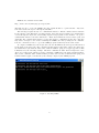
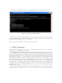
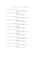
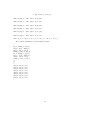
CoSBiLab LIME
User Manual
Ozan Kahramanoğulları, Ferenc Jordán and James Lynch
The Microsoft Research - University of Trento
Centre for Computational and Systems Biology
[email protected]
Version 1.0
Date 24/06/2010
.
You may use, copy, reproduce and distribute this software for any non-commercial
purpose, subject to the restrictions in CoSBi-SSLA. This software comes ‘as is’,
with no warranties. This means no express, implied or statutory warranty, including without limitation, warranties of merchantability or fitness for a particular
purpose, any warranty against interference with your enjoyment of the software
or any warranty of title or noninfringement. There is no warranty that this software will fulfilll any of your particular purposes or needs. Also, you must pass
this disclaimer on whenever you distribute the software or derivative works.
LIME User’s Guide
1
Introduction
LIME is a software aid for individual-based modeling of ecosystems. It enables ecologists to
describe ecosystem dynamics in a simple, intuitive language, which is then translated into a
format readable by the BlenX simulator. BlenX outputs some data files that can be used to
analyze and visualize the results of the simulation. Because BlenX is a very powerful and
general software tool, its input language is necessarily quite complicated and not easy to learn.
LIME is tailored toward ecosystem modeling, and users with no background in programming
can use it almost immediately. Figure 1 illustrates the flow of data in this process. The user
is directly concerned only with the LIME source code; the BlenX output files are processed by
other programs in the BetaWB suite.
Figure 1: LIME and BlenX Data Flow
The Appendix shows an example of the use of LIME and BlenX on a simple metacommunity
model.
2
Getting Started
Before using LIME, the user must install the BetaWB suite. This package is available for free
from the CoSBi website:
http://www.cosbi.eu/index.php/research/prototypes/beta-wb
1
LIME is also available from CoSBi:
http://www.cosbi.eu/index.php/prototypes/lime
The first step is to create the LIME source file, which should be a plain text file. Any basic
text editor such as Notepad or Wordpad will suffice.
The next steps require the use of a command line interface. This is a window that is available
in all versions of the Windows operating system. The user interacts with it by entering lines
of text through the keyboard, and reading output from programs on the monitor. To open a
command line interface, the user clicks Start → Run, enters cmd in the text box that opens, and
clicks OK. The command line interface opens, and awaits a command from the user. The user
may want to navigate to the folder containing the LIME source file by using the cd command.
It is also convenient to have a copy of the LIME program (lime.exe) in the same folder.
To compile a LIME source file and produce the two BlenX files, the user types lime followed
by the name of the source file. The convention is that whatever the name of the source file is, the
two BlenX files begin with the same name, with the suffixes .prog and .types appended. This
is illustrated by the following example. The first command cd lime files changes the active
directory to lime files, which is a folder containing a LIME source file named lotkavolterra.
The second command lime lotkavolterra produces the two files lotkavolterra.prog and
lotkavolterra.types, as indicated by the message output by the LIME program.
Figure 2: Invoking LIME
2
Still using a command line interface, the BlenX simulator (sim.exe) is then invoked:
Figure 3: Invoking the BlenX Simulator
There are two versions of the simulator, one for a 32-bit PC, and one for a 64-bit PC. The
results of the simulator are saved in several output files, which can then be analyzed with other
programs in the BetaWB package. For details see
http://www.cosbi.eu/index.php/research/prototypes/beta-wb
3
LIME Commands
Command names and names of species cannot contain blank spaces, and they are case sensitive.
This is also true of LIME source file names.
The LIME source file consists of five sections that specify the dynamics and spatial structure
of the ecosystem. Each section begins with a keyword that identifies the section. The space of the
system is organized into discrete regions called patches. The second and third sections specify
the dynamics within each patch, and the fourth section describes migrations between patches.
The system is stochastic, i.e., these changes are discrete events that occur unpredictably but
with certain probabilities. The rate of a change is a measure of how soon it is likely to occur.
The larger the rate is, the sooner the change is likely to occur. It is not a probability because
it can be any nonnegative real value. In fact, BlenX allows the rate to be +∞, which means
the change will occur instantaneously. Instantaneous waiting times are not used in LIME. More
technically, the waiting time until the change occurs is an exponential random variable whose
parameter is the rate, and consequently the reciprocal of the rate is the average waiting time
until the change occurs.
If the rate of a particular change depends on the patch in which it occurs, then there must be
a LIME command specifying the rate for each patch. But if the rate is the same for all patches,
3
one command (which does not mention any patch) suffices. This feature is called distributivity,
and can be applied to any command in section two or three.
In addition, if all the birth and death rates are 0, then section three can be omitted. Similarly,
if there are no migrations between patches, then section four can be omitted. If no command in
any section mentions a patch, then the system has one unnamed patch.
3.1
Duration Section
This section consists of one line which describes the length of time that the simulation will run.
It has two forms:
duration time tt.tt
or
duration steps nn
In the first instance, tt.tt is a real number denoting the total running time of the simulated
process. In the second, nn is the number of changes that the process undergoes before terminating.
3.2
Interactions Section
Following the keyword interactions are lines of text that specify the dynamics of the foodweb and other interactions between pairs of individuals. There are four types of interactions,
illustrated by these examples:
A eats B with rates xx.xx and yy.yy in P
Here, A and B are predator and prey respectively, and P is the name of a patch. There
are two possible outcomes of a predation event: either A simply kills B with rate xx.xx,
or A kills B and reproduces with rate yy.yy.
A facilitates B with rate xx.xx in P
Within patch P, A has a beneficial effect on B, causing B to reproduce with rate xx.xx.
Omitting "in P" distributes the rate over all patches.
A and B compete with rate xx.xx in P
Within patch P, A and B are mutually antagonistic, and both individuals will die as the
result of an interaction. Omitting "in P" distributes the rate over all patches.
A pollinates B with rates xx.xx and yy.yy in P
Within patch P, pollination of B by A causes A to reproduce with rate xx.xx and B to
reproduce with rate yy.yy. Omitting "in P" distributes the rate over all patches.
In any of these commands, the phrase "in P" can be omitted, meaning that the rate is
distributed throughout all patches.
3.3
Birth and Death Dynamics Section
The first line reads birth and death dynamics. The succeeding lines of text specify the birth
and death rates of the various species in each patch:
A is born with rate xx.xx in P
A dies with rate xx.xx in P
Again, if the patch is not specified, then the birth and/or death rates are distributed over all
patches for that species.
4
3.4
Patch Dynamics Section
This section begins with a line that reads patch dynamics, followed by commands that specify
the migration rates. These rates do not need to be the same in each direction:
A moves from P to Q with rate xx.xx
A moves from Q to P with rate yy.yy
3.5
Initial Population Section
Following a line that reads initial population, are lines that specify the starting populations
for each species:
nn A in P
where nn is the initial population size of species A in patch P.
3.6
Comments
Any line beginning with a double slash “//” is a comment and has no effect on the specification
of the model. Comments have at least two uses. First, even though LIME code is not difficult to
read, there could be sections of code whose purpose is not obvious, and comments could clarify
them. Second, comments provide an easy way to temporarily delete commands without erasing
them, simply by inserting double backslashes at their beginning.
4
Errors
If there are syntactic errors in the source file, then LIME cannot generate the BlenX input files.
Instead, error messages are displayed on the monitor to help the user find and correct the errors.
Typical errors involve incomplete, redundant, or contradictory specifications, as these examples
show:
1. Species A are in the ‘initial population’,
but they are not declared in the ‘interaction dynamics’.
There is a mismatch between the species declared in the ‘interactions’
and the ‘initial populations’ parts.
These two sets of species should be the same.
2. Empty Patch: undeclared patches in ‘initial population’.
These patches are not declared in the ‘interactions’ part.
3. There are two sentences for the plant-pollinator interaction
for the species A and B in patch P.
4. There are two sentences for the birth of the species A in patch P.
5. There are two sentences for the initial quantity of the species A in patch P.
6. There are two sentences for the movement of the species A from patch P to Q.
7. No interaction is specified. Interactions cannot be empty.
5
8. Species A are in the ‘initial population’,
but they are not declared in the ‘interaction dynamics’.
There is a mismatch between the species declared in the ‘interactions’
and the ‘initial populations’ parts.
These two sets of species should be the same.
9. The identifier A is used to denote both a patch and a species.
The identifiers that describe patches and species should be different.
5
Examples
The following examples are not intended to be biologically significant; rather, they illustrate the
process of developing a model by starting with a simple system and repeatedly correcting errors
and adding more details. The model has three species: a plant (daylily), a pollinator of the plant
(bumblebee), and a predator (bluejay). The first version has only one patch and an error:
duration steps 1000
interactions
BumbleBee pollinates DayLily with rates 1 and 2
BlueJay eats BumbleBee with rates 0.2 and 0.1
birth and death dynamics
DayLily is born with rate 1
DayLily dies with rate 1
BumbleBee is born with rate 0.5
BumbleBee dies with rate 0.6
BlueBird is born with rate 0.1
BlueJay dies with rate 0.11
initial population
10 DayLily
100 BumbleBee
5 BlueJay
When it is input to LIME, an error message is produced:
BlueBird: undeclared species in ‘birth and death dynamics’.
These species are not declared in the ‘interactions’ part.
After ‘BlueBird’ is changed to ‘BlueJay’ in line 12, LIME can rerun the source file, and this
time it will successfully generate the .prog and types files.
Next, the model is augmented by specifying three patches:
duration steps 1000
interactions
BumbleBee pollinates DayLily with rates 1 and 2 in CenterPatch
6
BumbleBee pollinates DayLily with rates 1 and 2 in LeftPatch
BumbleBee pollinates DayLily with rates 1 and 2 in RightPatch
// BlueJay’s feeding rate is distributed over all patches
BlueJay eats BumbleBee with rates 0.2 and 0.1
birth and death dynamics
DayLily is born with rate 1 in CenterPatch
DayLily dies with rate 1 in CenterPatch
BumbleBee is born with rate 0.5 in CenterPatch
BumbleBee dies with rate 0.6 in CenterPatch
DayLily is born with rate 1.2 in LeftPatch
DayLily dies with rate 1 in LeftPatch
BumbleBee is born with rate 0.5 in RightPatch
BumbleBee dies with rate 0.6 in RightPatch
// BlueJay’s birth and death rates are distributed over all patches.
BlueJay is born with rate 0.1
BlueJay dies with rate 0.11
patch dynamics
DayLily moves from CenterPatch to LeftPatch with rate 2.0
DayLily moves from LeftPatch to CenterPatch with rate 2.0
BumbleBee moves from CenterPatch to LeftPatch with rate 1.0
BumbleBee moves from LeftPatch to CenterPatch with rate 0.5
BlueJay moves from CenterPatch to LeftPatch with rate 0.8
BlueJay moves from LeftPatch to CenterPatch with rate 0.3
initial population
// Only CenterPatch is initially occupied.
10 DayLily in CenterPatch
100 BumbleBee in CenterPatch
5 BlueJay in CenterPatch
When it is input to LIME, the .prog and types files are generated, but because the patch
named Rightpatch is isolated from the other patches, warnings are generated:
Warning:
Warning:
Warning:
patch CenterPatch is isolated from the patches RightPatch.
patch LeftPatch is isolated from the patches RightPatch.
patch RightPatch is isolated from the patches CenterPatch, LeftPatch.
Warnings are not necessarily errors, but they inform the user of possibly unintended consequences. The patches can be connected by adding some commands to the patch dynamics section:
DayLily moves from CenterPatch to RightPatch with rate 2.0
DayLily moves from RightPatch to CenterPatch with rate 2.0
BumbleBee moves from CenterPatch to RightPatch with rate 1.0
BumbleBee moves from RightPatch to CenterPatch with rate 0.5
BlueJay moves from CenterPatch to RightPatch with rate 0.8
7
BlueJay moves from RightPatch to CenterPatch with rate 0.3
Appendix: Example of LIME and BlenX Applied to a Model
Ecosystem.
Figure 4: The simplistic metacommunity model with three species (A, B and C) in two identical
habitat patches (X and Y). A and B prey on C with rates 0.4 and 0.8, respectively. Only species
A migrates with rate m = 1. Death rate for both A and B in both patches equals d = 0.0001,
while birth rate for C in both patches equals b = 10. Initial population sizes are given by t0
equalling 5 for A and B, whilet0 equals 15 for C.
The user-friendly LIME model specification to be translated into BlenX.
duration steps 2000
interactions
A eats C with
B eats C with
A eats C with
B eats C with
rates
rates
rates
rates
0.4
0.8
0.4
0.8
and
and
and
and
0.4
0.8
0.4
0.8
in
in
in
in
X
X
Y
Y
birth and death dynamics
A dies with rate 0.0001 in X
B dies with rate 0.0001 in X
8
C
A
B
C
is born with rate 10 in X
dies with rate 0.0001 in Y
dies with rate 0.0001 in Y
is born with rate 10 in Y
patch dynamics
A moves from X to Y with rate 1.0
A moves from Y to X with rate 1.0
initial population
5 A in X
5 B in X
15 C in X
5 A in Y
5 B in Y
15 C in Y
The translated PROG file of the BlenX programme.
[ steps = 2000 ]
<< BASERATE:inf >>
let A_Prog : pproc =
if (ex,Aex_X) then ex!().start!() endif
+ if (ey,Aey_X) then ey!().ch(r,ArRep_X) endif
+ if (ex,Aex_Y) then ex!().start!() endif
+ if (ey,Aey_Y) then ey!().ch(r,ArRep_Y) endif
+ if (ex,Aex_X) then delay(1.0).ch(r,Ar_Y).
ch(ex,Aex_Y).ch(ey,Aey_Y).start!() endif
+ if (ex,Aex_Y) then delay(1.0).ch(r,Ar_X).
ch(ex,Aex_X).ch(ey,Aey_X).start!() endif
+ if (ex,Aex_X) then die(0.00010) endif
+ if (ex,Aex_Y) then die(0.00010) endif
;
let B_Prog : pproc =
if (ex,Bex_X)
+ if (ey,Bey_X)
+ if (ex,Bex_Y)
+ if (ey,Bey_Y)
+ if (ex,Bex_X)
+ if (ex,Bex_Y)
;
let C_Prog : pproc =
if (ex,Cex_X)
+ if (ey,Cey_X)
+ if (ex,Cex_Y)
+ if (ey,Cey_Y)
+ if (ex,Cex_X)
then
then
then
then
then
then
ex!().start!() endif
ey!().ch(r,BrRep_X) endif
ex!().start!() endif
ey!().ch(r,BrRep_Y) endif
die(0.00010) endif
die(0.00010) endif
then
then
then
then
then
ex?().die(inf) endif
ey?().die(inf) endif
ex?().die(inf) endif
ey?().die(inf) endif
ch(10.0,r,CrRep_X) endif
9
+ if (ex,Cex_Y) then ch(10.0,r,CrRep_Y) endif
;
let A_X : bproc = #(r,Ar_X),
#(ex,Aex_X), #(ey,Aey_X)
[ rep start?().A_Prog | A_Prog ];
let A_Rep_X : bproc = #(r,ArRep_X),
#(ex,Aex_X), #(ey,Aey_X)
[ rep start?().A_Prog ];
let A_Y : bproc = #(r,Ar_Y),
#(ex,Aex_Y), #(ey,Aey_Y)
[ rep start?().A_Prog | A_Prog ];
let A_Rep_Y : bproc = #(r,ArRep_Y),
#(ex,Aex_Y), #(ey,Aey_Y)
[ rep start?().A_Prog ];
let B_X : bproc = #(r,Br_X),
#(ex,Bex_X), #(ey,Bey_X)
[ rep start?().B_Prog | B_Prog ];
let B_Rep_X : bproc = #(r,BrRep_X),
#(ex,Bex_X), #(ey,Bey_X)
[ rep start?().B_Prog ];
let B_Y : bproc = #(r,Br_Y),
#(ex,Bex_Y), #(ey,Bey_Y)
[ rep start?().B_Prog | B_Prog ];
let B_Rep_Y : bproc = #(r,BrRep_Y),
#(ex,Bex_Y), #(ey,Bey_Y)
[ rep start?().B_Prog ];
let C_X : bproc = #(r,Cr_X),
#(ex,Cex_X), #(ey,Cey_X)
[ rep start?().C_Prog | C_Prog ];
let C_Rep_X : bproc = #(r,CrRep_X),
#(ex,Cex_X), #(ey,Cey_X)
[ rep start?().C_Prog ];
let C_Y : bproc = #(r,Cr_Y),
#(ex,Cex_Y), #(ey,Cey_Y)
[ rep start?().C_Prog | C_Prog ];
let C_Rep_Y : bproc = #(r,CrRep_Y),
#(ex,Cex_Y), #(ey,Cey_Y)
10
[ rep start?().C_Prog ];
when (A_Rep_X: :inf) split (A_X,A_X);
when (A_Rep_Y: :inf) split (A_Y,A_Y);
when (B_Rep_X: :inf) split (B_X,B_X);
when (B_Rep_Y: :inf) split (B_Y,B_Y);
when (C_Rep_X: :inf) split (C_X,C_X);
when (C_Rep_Y: :inf) split (C_Y,C_Y);
run 5 A_X || 5 B_X || 15 C_X || 5 A_Y || 5 B_Y || 15 C_Y
The translated TYPE file of the BlenX programme.
{
Ar_X, ArRep_X, Aex_X,
Aey_X, Ar_Y, ArRep_Y,
Aex_Y, Aey_Y, Br_X,
BrRep_X, Bex_X, Bey_X,
Br_Y, BrRep_Y, Bex_Y,
Bey_Y, Cr_X, CrRep_X,
Cex_X, Cey_X, Cr_Y,
CrRep_Y, Cex_Y, Cey_Y
}
%%
{
(Aex_X,Cex_X,0.40),
(Aex_Y,Cex_Y,0.40),
(Aey_X,Cey_X,0.40),
(Aey_Y,Cey_Y,0.40),
(Bex_X,Cex_X,0.80),
(Bex_Y,Cex_Y,0.80),
(Bey_X,Cey_X,0.80),
(Bey_Y,Cey_Y,0.80)
}
11
Figure 5: The population size of three species in two habitat patches during the simulation. (a)
shows patch X (A: yellow, B: blue, C: red) and (b) shows patch Y (A: grey, B: red, C: green).
12