Download TOCHNOG PROFESSIONAL Tutorial manual Version 23

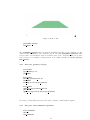
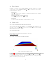
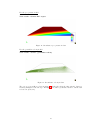
TOCHNOG PROFESSIONAL Tutorial manual
Version 23
Dennis Roddeman
December 7, 2015
1
Contents
1 Conditions
5
2 Basic information
6
3 Tutorial 1: slope safety factor analysis
7
3.1
Mesh generation with Gid . . . . . . . . . . . . . . . . . . . . . . . . . . . . . . . .
7
3.2
Input file . . . . . . . . . . . . . . . . . . . . . . . . . . . . . . . . . . . . . . . . .
8
3.2.1
Initialization part . . . . . . . . . . . . . . . . . . . . . . . . . . . . . . . . .
9
3.2.2
Data part, geometry of edges . . . . . . . . . . . . . . . . . . . . . . . . . .
9
3.2.3
Data part, boundary conditions . . . . . . . . . . . . . . . . . . . . . . . . .
10
3.2.4
Data part, gravity . . . . . . . . . . . . . . . . . . . . . . . . . . . . . . . .
10
3.2.5
Data part, material properties . . . . . . . . . . . . . . . . . . . . . . . . .
11
3.2.6
Data part, prepare post-processing . . . . . . . . . . . . . . . . . . . . . . .
12
3.2.7
Data part, apply gravity time-steps . . . . . . . . . . . . . . . . . . . . . . .
12
3.2.8
Data part, apply safety factor calculation time-steps . . . . . . . . . . . . .
13
3.2.9
Data part, include mesh generated with Gid . . . . . . . . . . . . . . . . . .
13
3.2.10 Data part, final remarks for advanced users . . . . . . . . . . . . . . . . . .
13
3.3
Run calculation . . . . . . . . . . . . . . . . . . . . . . . . . . . . . . . . . . . . . .
14
3.4
Output results . . . . . . . . . . . . . . . . . . . . . . . . . . . . . . . . . . . . . .
14
3.4.1
Determine safety factor . . . . . . . . . . . . . . . . . . . . . . . . . . . . .
14
3.4.2
Plot displacement history in Gnuplot . . . . . . . . . . . . . . . . . . . . . .
14
3.4.3
Plot results in Gid . . . . . . . . . . . . . . . . . . . . . . . . . . . . . . . .
15
4 Tutorial 2: non-saturated dam with seepage edge
17
4.1
Mesh generation with Gid . . . . . . . . . . . . . . . . . . . . . . . . . . . . . . . .
17
4.2
Input file . . . . . . . . . . . . . . . . . . . . . . . . . . . . . . . . . . . . . . . . .
17
4.2.1
Initialization part . . . . . . . . . . . . . . . . . . . . . . . . . . . . . . . . .
17
4.2.2
Data part, geometry of edges . . . . . . . . . . . . . . . . . . . . . . . . . .
18
4.2.3
Data part, some arithmetic expressions . . . . . . . . . . . . . . . . . . . .
18
4.2.4
Data part, gravity . . . . . . . . . . . . . . . . . . . . . . . . . . . . . . . .
19
4.2.5
Data part, groundwater . . . . . . . . . . . . . . . . . . . . . . . . . . . . .
19
2
4.2.6
Data part, boundary conditions on edges . . . . . . . . . . . . . . . . . . .
19
4.2.7
Data part, material properties . . . . . . . . . . . . . . . . . . . . . . . . .
20
4.2.8
Data part, prepare post-processing . . . . . . . . . . . . . . . . . . . . . . .
20
4.2.9
Data part, apply linear time-steps . . . . . . . . . . . . . . . . . . . . . . .
21
4.2.10 Data part, apply nonlinear time-steps . . . . . . . . . . . . . . . . . . . . .
21
4.2.11 Data part, include mesh generated with Gid . . . . . . . . . . . . . . . . . .
21
4.2.12 Data part, final remarks for advanced users . . . . . . . . . . . . . . . . . .
21
4.3
Run calculation . . . . . . . . . . . . . . . . . . . . . . . . . . . . . . . . . . . . . .
22
4.4
Output results . . . . . . . . . . . . . . . . . . . . . . . . . . . . . . . . . . . . . .
22
4.4.1
Value of the groundwater flux out of the left edge . . . . . . . . . . . . . . .
22
4.4.2
Plot results in Gid . . . . . . . . . . . . . . . . . . . . . . . . . . . . . . . .
22
5 Tutorial 3: excavation with sheet pile, beam and contact spring elements
5.1
5.2
24
Input file . . . . . . . . . . . . . . . . . . . . . . . . . . . . . . . . . . . . . . . . .
24
5.1.1
Initialization part . . . . . . . . . . . . . . . . . . . . . . . . . . . . . . . . .
24
5.1.2
Data part, tolerance on geometries . . . . . . . . . . . . . . . . . . . . . . .
25
5.1.3
Data part, beam geometries . . . . . . . . . . . . . . . . . . . . . . . . . . .
25
5.1.4
Data part, edge geometries . . . . . . . . . . . . . . . . . . . . . . . . . . .
26
5.1.5
Data part, excavation geometries . . . . . . . . . . . . . . . . . . . . . . . .
26
5.1.6
Data part, material properties . . . . . . . . . . . . . . . . . . . . . . . . .
27
5.1.7
Data part, boundary conditions . . . . . . . . . . . . . . . . . . . . . . . . .
28
5.1.8
Data part, distributed force load on top . . . . . . . . . . . . . . . . . . . .
28
5.1.9
Data part, gravity . . . . . . . . . . . . . . . . . . . . . . . . . . . . . . . .
29
5.1.10 Data part, groundwater properties . . . . . . . . . . . . . . . . . . . . . . .
29
5.1.11 Data part, post processing and printing . . . . . . . . . . . . . . . . . . . .
29
5.1.12 Data part, generate mesh with Tochnog . . . . . . . . . . . . . . . . . . . .
30
5.1.13 Data part, set gravity stresses . . . . . . . . . . . . . . . . . . . . . . . . . .
31
5.1.14 Data part, apply excavation time-steps . . . . . . . . . . . . . . . . . . . . .
33
5.1.15 Data part, apply load time-steps . . . . . . . . . . . . . . . . . . . . . . . .
34
5.1.16 Data part, apply velocity point A time-steps . . . . . . . . . . . . . . . . .
34
5.1.17 Data part, print pressure on beam . . . . . . . . . . . . . . . . . . . . . . .
34
Run calculation . . . . . . . . . . . . . . . . . . . . . . . . . . . . . . . . . . . . . .
35
3
5.3
Output results . . . . . . . . . . . . . . . . . . . . . . . . . . . . . . . . . . . . . .
6 Tutorial 4: excavation with sheet pile, isoparametric and interface elements
6.1
35
38
Input file . . . . . . . . . . . . . . . . . . . . . . . . . . . . . . . . . . . . . . . . .
38
6.1.1
Initialization part . . . . . . . . . . . . . . . . . . . . . . . . . . . . . . . . .
38
6.1.2
Data part, using linear test calculations . . . . . . . . . . . . . . . . . . . .
38
6.1.3
Data part, geometries . . . . . . . . . . . . . . . . . . . . . . . . . . . . . .
39
6.1.4
Data part, material properties . . . . . . . . . . . . . . . . . . . . . . . . .
39
6.1.5
Data part, generate mesh with Tochnog . . . . . . . . . . . . . . . . . . . .
39
6.1.6
Data part, post processing and printing . . . . . . . . . . . . . . . . . . . .
40
6.1.7
Data part, timesteps . . . . . . . . . . . . . . . . . . . . . . . . . . . . . . .
41
6.2
Run calculation . . . . . . . . . . . . . . . . . . . . . . . . . . . . . . . . . . . . . .
42
6.3
Output results . . . . . . . . . . . . . . . . . . . . . . . . . . . . . . . . . . . . . .
42
4
1
Conditions
All conditions from the Tochnog Order form apply. See our internet page for the latest order form.
5
2
Basic information
The tutorials in this manual describe calculations in decreasing detail. The first tutorial discusses
many aspects, whereas the following tutorials discuss less aspects. You can find these tutorials on
your distribution in the directory tochnog/test/tutorial.
Mesh preparation and post-processing is done with Gid 7.6.0b under Linux. Gid is copyrighted by
CIMNE, see http://www.gidhome.com. It is advised to learn Gid first.
The advanced user under Linux can also find examples on how specific input commands are used
by grepping in the tochnog test input files in the tochnog/test/other directory, e.g. grep
control timestep *.dat.
6
3
Tutorial 1: slope safety factor analysis
This tutorial is taken from example 2 in [1]. The safety factor of a slope is calculated.
20
20
5
15
20
60
Figure 1: Slope
Figure 1 shows the slope. The lower edge is completely fixed, whereas at the left and right edge
free sliding in vertical direction is allowed.
3.1
Mesh generation with Gid
Although Tochnog contains some build in mesh generation, here for generality the external Pre-and
Postprocessor Gid is used. Start Gid and perform the following steps.
Specify the Tochnog problem type in Gid
Data - Problem type - Tochnog
This takes care that Gid understands that you want to generate a mesh for Tochnog. Some Tochnog
specific input is now available, and once the mesh is generated it can be written in a file in Tochnog
specific format.
Create points, lines and a surface in Gid
Geometry - Create - Point
Create the points along the entire edge of the slope, thus (0,0), (60,0), (60,5), (40,5), (20,15) and
(0,15).
Zoom - Frame
Zoom to the total frame to see all points.
Geometry - Create - Straight Line
Use the points to create the straight lines along the entire edge.
Geometry - Create - Nurbs surface - By contour
Use the straight lines to create a surface. Figure 2 shows the Nurbs surface.
Assign a material to the surface
Data - Materials - Assign - Surfaces
Now assign to the surface a Tochnog element group (material). Select GROUP1 in the dialog,
and set the group type to -materi. Then select the surface with Assign Surfaces.
Generate a mesh with linear triangles
7
Figure 2: Nurbs surface of slope
Mesh - Generate mesh
Gid uses as default element type for surfaces linear triangles, which are OK for the slope stability
analysis. Hence we don’t need to change the element type, and can go straight on to generate the
mesh: Setting the element size to 0.5 gives a fine mesh, good enough for an accurate solution.
Figure 3: Mesh of slope
Save gid data
File - Save As - mesh.gid
Save everything to the directory mesh.gid.
Write file with tochnog elements, nodes and element groups (materials)
Calculate - Calculate
To really obtain the generated mesh in a file that can be used for Tochnog, calculate the Tochnog
file. Please realize that this option in Gid only calculates the Tochnog input file for the mesh , and
not does the FE calculation itself (solving equations, ...). In the directory mesh.gid you can find
the file mesh.dat which contains element , element group and node data.
The element data records contain the element number, the element name, here -tria3, and finally
the node numbers to which the element is connected. The element group records contain for
each element the group number which contains material properties for the element. The node
records contain for each node the coordinates.
3.2
Input file
The input file always contains two parts. The initialization part essentially specifies which unknown
fields need to be solved. The data part specifies elements, nodes, boundary conditions, etc.
8
3.2.1
Initialization part
echo -yes
number of space dimensions 2
materi velocity
materi displacement
materi stress
materi strain plasti
end initia
The first line echo -yes tells Tochnog that the input should be echoed when it is read. This is
convenient in locating errors in your input file: you can see up to which line the input file is read
before the error occurs. Use echo -no if you don’t want to echo the input file.
The number of space dimensions 2 specifies that the dimensionality of the calculation is 2D
(plane strain, plane stress, or axi-symmetric). Also 1 and 3 are available in Tochnog (thus 1D and
3D).
The materi velocity together with the materi displacement takes care that the velocity and
displacement fields are present for solution. Since this is a 2D calculation, only the x and y
components are present in the calculation.
Initialization of the stress field is done with materi stress. Please realism that all the 9 components σij of the 3D stress matrix are present in the calculation, since, by example in plane
strain, displacements in x and y also lead to σzz However, the stress matrix is symmetric, so only
6 components need actually to be stored for the stress field; the other components follow from
symmetry.
In this slope stability calculation an elasto-plastic material model will be used, and thus initialization of the plastic strains materi strain plasti is needed.
After you have run the calculation you can always see in the data record dof label in the database
file, in this case tutorial 1.dbs, the component names of the initialized dof’s (-disx and -disy
for the displacements materi displacement, etc.).
3.2.2
Data part, geometry of edges
start define
bottom edge geometry line 1
end define
start define
right edge geometry line 2
end define
start define
left edge geometry line 3
end define
We want to specify the edges at which boundary conditions are imposed later. Each edge will
be specified by a geometry line data record, since the edges are straight lines. It is convenient
to define a name for each edge, so that later that name can be used when needed and the input
9
file remains more readable. Each start define ... end define specifies a word, by example
bottom edge which will be later substituted with its real meaning, by example geometry line
1. Such defines can be used for all kinds of input.
bottom edge 0.0 0.0 60.0 0.0 0.01
left edge 0.0 0.0 0.0 15.0 0.01
right edge 60.0 0.0 60.0 5.0 0.01
The first line bottom edge 0.0 0.0 60.0 0.0 0.01 is read by Tochnog as geometry line 1
0.0 0.0 60.0 0.0 0.01, so in fact geometry line 1 is specified. The other two lines specify
geometry line 2 and geometry line 3. The 0.01 indicate the tolerance of the lines; all nodes
in the model with a distance not more than 0.01 are considered to be located on the geometrical
lines.
Notice that we identify each geometry line by a unique index; for the present geometry lines the
indices 1, 2 and 3 are used. In fact, most of the data in the input file uses an index, by example
element data records use an index which is the element number, node data records use an index
which is the node number, etc.
3.2.3
Data part, boundary conditions
bounda dof 0 -bottom edge -disx -disy
bounda dof 1 -left edge -disx
bounda dof 2 -right edge -disx
The bounda dof records are used to prescribe unknowns (dof’s). On the bottom edge the displacement in x-direction -disx and the displacement in y-direction -disy are suppressed, and on
the left edge and right edge the displacement in x-direction -disx is suppressed. The nice thing
about using geometries for boundary conditions is that these remain valid, even if you change the
mesh (amount of elements, nodes).
First side remark: if we want to apply a non-zero displacement then also the bounda time records
should be specified; here however displacements on the edges are zero, and then the bounda time
records are not needed.
Second side remark: if displacements are prescribed, velocities automatically are calculated by
Tochnog from the time derivative of the displacements. If you would prescribe velocities with
-velx and -vely then displacements automatically follow from time integration of the velocities.
Third side remark: a list of all unknown names like -disx etc. can be found at dof label in the
users manual. The dof label is available in the database file after the calculation.
3.2.4
Data part, gravity
force gravity 0.0 -10.
force gravity time 0.0 0.0 0.5 1.0 1.e20 1.0
The gravity components as specified in force gravity are 0 in x-directions, and −10. sm2 in ydirection. The force gravity time specifies at time versus factor diagram; this is the factor with
10
which the gravity is applied. It should be read as follows: at time 0.0 the factor is 0.0, at time 0.5
the factor is 1.0 and up to time 1.e20 the factor remains 1.0. Later in this tutorial, we will further
discuss this topic; so just go straight ahead with reading the next input.
Please realize that all input in Tochnog does not have a specific dimension. The user just should
take care that he/she uses consistent units for the different input data, but otherwise the units of
input data is not pre-defined.
3.2.5
Data part, material properties
start define
phi 0.349065
end define
start define
tanphi 0.3639
end define
start define
c 10.0
end define
First we define the soil friction angle φ = 0.349065 in radians (so 20 degrees), and the cohesion
c = 10.0 kN
m2 .
group
group
group
group
group
group
group
type 1 -materi
materi memory 1 -total linear
materi density 1 2.0
materi elasti young 1 1.e5
materi elasti poisson 1 0.3
materi plasti tension direct 1 10.0
materi plasti mohr coul direct 1 phi c 0.0
When we made the mesh with GID, all elements were assigned to group 1. Here we define the
material properties of group 1. The group type is set to -materi which means that material
strains, stresses, etc. will be solved. With group materi memory set to -total linear you
specify a classical geometrically linear (small deformations) approximation for the soil; this is sufficient for almost all typical calculations. The soil density is set to 2. 1000.kg
in the data record
m3
group materi density. The Young’s modulus and Poisson’s ratio are 1.e5 kN
m2 and 0.3, as set
in the records group materi elasti young and group materi elasti poisson respectively. For
shear failure the Mohr-Coulomb yield surface is used; the record group materi plasti mohr coul direct
specifies the friction angle φ, the cohesion c and zero dilatancy. To include tension failure (limitation
of tensile stress in soils), you explicitely need to include group materi plasti tension direct in
the input file; here the maximum tensile stress is set to 10.0 kN
m2 .
change
change
change
change
dataitem
dataitem
dataitem
dataitem
10 -group materi plasti mohr coul direct 1 0 -use
time 10 0.0 tanphi 1.0 tanphi 2.0 0. 1.e20 0.0
time method 10 -tangent
20 -group materi plasti mohr coul direct 1 1 -use
11
change dataitem time 20 0.0 c 1.0 c 2.0 0.0 1.e20 0.0
The change dataitem and change dataitem time records take care that the friction angle and
cohesion are lowered in the calculation, so that we find the minimum friction angle and cohesion
for stability. The ratio of the start values and the minimum values will define the safety factor.
The change dataitem 10 record specifies for the group materi plasti mohr coul direct record
with index 1 (so group 1) and ’number 0’. With ’number 0’ the first value in the group materi plasti mohr co
is meant, thus the friction angle. The diagram in change dataitem time 10 specifies that at
time 0.0 the friction angle is the predefined word phi (thus 0.349065), at time 1.0 it is again the
predefined word phi, at time 2.0 it is 0.0 and at time 1.0e20 it is 0.0. Between the specified time
points the value will be linearly interpolated. The -use specifies that the given values should
actually be used (as opposed to other options, see the users manual).
Similarly the cohesion is varied in time with change dataitem 20 and change dataitem time
20.
3.2.6
Data part, prepare post-processing
post point 10 20.0 15.0
With post point 10 a point in the domain is defined, at which Tochnog will monitor during the calculation solution fields. The solution field at the point will be placed in the record post point dof
10. Such post point dof record in turn can be used in several printing options.
3.2.7
Data part, apply gravity time-steps
control timestep 10 1.e-1 1.0
control print 10 -time current -post node rhside ratio
control print gid 20 -yes
control reset dof 30 -disx -disy -eppxx -eppxy -eppxz -eppyy -eppyz -eppzz
Time-steps are actually started with control timestep 10. There is one important topic about
all control * records that we need to discuss first. These control * records also have an index, here the indices are 10, 20 and 30. Specifically for control * records these indices are
important: these records will be performed in order of increasing index. Here that means that
the records control timestep 10 and control print 10 are performed first, after that the record
control print gid 20 is performed, and after that the record control reset dof 30 is performed.
The control timestep 10 record tells Tochnog to take time-steps of size 0.1 until a total time increment of 1.0 is obtained. The control print 10 record specifies that some data records need to be
printed, specifically the current time -time current and the accuracy ratio -post node rhside ratio.
The accuracy ratio contains the maximum out-of-balance force on a free node (that is a node without prescribed displacement) divided by the maximum external force on a node with prescribed
displacement. Normally all printing during a calculation goes to the computer monitor (but the
advanced user can redirect printed output to a file).
Now look back at how we defined the gravity in time. It was increased from 0.0 at time 0.0 to its
final value of 10 at time 0.5. Thus, the time increment of 1.0 is enough for getting gravity imposed
12
(from time 0.0 to time 0.5), and also allows the equilibrium with full gravity to be established
accurately with additional time-steps (from time 0.5 to time 1.0).
The control print gid 20 record takes care that the results at the end of gravity are printed in
the tochnog flavia.msh and tochnog flavia.res files. These can be post-processed with Gid.
Finally, to prepare the safety factor calculation itself, some results are set to 0.0 in order to be able
to distinguish clearly after the safety factor calculation between safety factor results (instability
results) and gravity results. To be specific, the displacement components -disx, -disy are set to
0.0 and the components of the plastic strains -eppxx -eppxy -eppxz -eppyy -eppyz -eppzz
are set to 0.0.
3.2.8
Data part, apply safety factor calculation time-steps
control
control
control
control
timestep 40 1.e-4 1.0
timestep iterations automatic 40 1.e-3 1.e-5 1.e-2
print 40 -time current -post node rhside ratio
print history 40 -post point dof 10 -disy
control print gid 50 -yes
Look first back at the material definition where the friction angle and cohesion are lowered between
time 1 and time 2. We will now use time-steps to determine where between time 1 and 2 the slope
becomes unstable. The records control timestep 40 with control timestep iterations automatic
40 together define automatic time-steps, which will be taken till instability occurs. The record
control timestep defines an initial timestep of 1.e-4 and total time increment of 1.0. The record
control timestep iterations automatic specifies that the maximum allowed value of the error
ratio -post node rhside ratio is 1.e-3, the minimum allowed time-step size is 1.e-5 and the maximum allowed time-step size is 1.e-2. Tochnog will decrease the time-step size if that is needed to
keep the error ratio below 1.e-3. If that is not possible anymore, due to instability caused by low
friction angle and cohesion, the calculation is terminated. Later we will discuss how, using the
current time of the terminated calculation, the safety factor can be calculated.
3.2.9
Data part, include mesh generated with Gid
include mesh.gid/mesh.dat
The include command allows you to include other files containing data records in the current
input file. Here the mesh data as generated with Gid is included.
3.2.10
Data part, final remarks for advanced users
solver matrix save -always
Default Tochnog will completely setup and decompose the system matrix when it thinks the matrix
is changed. In the present calculation some material data is changed (the friction angle and
cohesion), and so Tochnog will setup and decompose the system matrix at all time-steps between
time 1.0 and 2.0. You can impose, however, that the matrix will not be setup and decomposed
each time-step by using solver matrix save -always; then the decomposed matrix is saved once,
13
and used again at the next time-step. This can save considerable computing time. This typically
is useful for safety factor calculations, but otherwise should only be used with care.
target item 10 -time current 0 0
target value 10 1.0 2.e-2
The records target item and target value are a convenient method to check if critical results of
a calculation do change. With target item you specify which result should be checked, and with
target value you specify the expected value maximum allowed deviation from the result. In case
the real value differs more from the expected value, here 1.0, then the maximum deviation, here
2.e-2, an error message is printed in the file tochnog.log.
In this way you can make your own set of calculations which are important for your applications,
and check with each new tochnog release if results are still like you expect them to be.
3.3
Run calculation
On Linux open a window, and type in the directory with the tutorial 1 input file the command
tochnog tutorial 1. On Microsoft Windows open a DOS command prompt, and type in the
directory with the tutorial 1 input file the command tochnog.exe tutorial 1.
After the calculation is ready you will see the following extra files in the directory:
• tutorial 1.dbs
This is the database after the calculation. It contains all information from the calculation
(input data, results, etc.).
• tutorial 1 flavia.msh and tutorial 1 flavia.res
Post-processing files which can be opened with Gid.
• tochnog.log
Log file from Tochnog which lists the calculations that have been run.
• post point dof 10 disy.his
History file with time versus y-displacement for the post point 10.
3.4
3.4.1
Output results
Determine safety factor
You will see that at time 1.36 the friction angle and cohesion have become such low that the slope
becomes unstable. At that time the cohesion has decreased from 10.0 kN
m2 to (1. − 0.36) ∗ 10.0 =
kN
10
6.4 m2 . The safety factor thus is 6.4 = 1.56.
3.4.2
Plot displacement history in Gnuplot
A history plot of the vertical displacement of the post point in the file ”post point dof 10 disy.his”
shows what is happening when the cohesion and friction angle are lowered in time between 1.0 and
2.0. Here we use Gnuplot as plotting program, but since the file ”post point dof 10 disy.his”
14
is a simple ASCII text file you can use any program of your preference for plotting. With Gnuplot
do the following for getting a postscript result of the displacement history:
gnuplot
p ”post point dof 10 disy.his” with lines
set term postscript
set output ”post point dof 10 disy.ps”
replot
0
"post_point_dof_10_disy.his"
-0.002
-0.004
-0.006
-0.008
-0.01
-0.012
-0.014
-0.016
-0.018
-0.02
1
1.05
1.1
1.15
1.2
1.25
1.3
Figure 4: Vertical displacement of post point in time
Clearly finally the slope becomes unstable.
3.4.3
Plot results in Gid
Open in Gid results
View - Postprocess
File - Open
tutorial 1 flavia.msh
View - Zoom - In
In Gid you first need to open the Gid results files as written by Tochnog, and then zoom in to get
the slope full in the figure.
Plot boundary conditions in Gid
View results - Display Vectors - materi bounda dof - All
Tochnog also writes information about boundary conditions, external forces, etc. in the Gid postprocessing files. In the present example, you can look in Gid at the boundary conditions with the
command as given above.
Plot gravity results
View results - Default Analysis/Step - time - 1.
15
Figure 5: Boundary conditions
View results - Contour Fill - materi stress - sigyy
Figure 6: Vertical stress
These commands show how you obtain in Gid a contour filled plot of the vertical stress field after
gravity is imposed (time 1.0).
Plot safety results
View results - Default Analysis/Step - time - 1.32
Windows - View Style - Style - All Lines
View results - Display Vectors - materi velocity - | materi velocity |
The velocity profile at instability clearly shows how a circular segment slides away. It is evident
that the Mohr-Coulomb shear failure condition with reduced cohesion and friction angle causes
this instability.
16
4
Tutorial 2: non-saturated dam with seepage edge
This tutorial shows how to perform a non-saturated groundflow analysis in a dam. Figure 7 shows
the dam.
55
65
45
30
20
165
Figure 7: Dam
At the lower part of the right edge a water level of 20m is present, by example because of a
lake. The lower edge of the dam does not allow for inward or outward flow of ground water, it is
non-permeable. The left edge is a seepage edge, it only allows for outward water flow and not for
inward water flow.
4.1
Mesh generation with Gid
The mesh generation in Gid is very similar to tutorial 1, so it is not repeated here. We just remark
that the element size, as required in the Gid Mesh - Generate dialog should be set to 1.0 to get
a reasonably fine mesh.
Figure 8: Nurbs surface of dam
Figure 8 shows the Nurbs surface. Figure 9 shows the mesh.
4.2
4.2.1
Input file
Initialization part
echo -yes
number of space dimensions 2
groundflow pressure
groundflow saturation
17
Figure 9: Mesh of dam
groundflow velocity
end initia
The groundflow pressure takes care that the hydraulic head field becomes available over the
entire domain. Initialization of the saturation rate is done with groundflow saturation. This
is needed since a non-saturated water model will be used. It is convenient to have the groundflow velocity vectors available for interpretation of the results, and thus we initialize groundflow velocity.
4.2.2
Data part, geometry of edges
start define
eps geometry 1.e-1
end define
start define
left edge geometry line 10
end define
left edge 0 0 55 30 eps geometry
start define
right dry edge geometry line 20
end define
right dry edge 135 20 120 30 eps geometry
We define geometrical lines where later the water boundary conditions will be applied.
4.2.3
Data part, some arithmetic expressions
start arithmetic
rho 1.0
end arithmetic
18
start arithmetic
g -10.0
end arithmetic
start arithmetic
g absolute 10.0
end arithmetic
Here some parameters are specified with start arithmetic ... end arithmetic. The advantage
of such arithmetic definitions for floating point parameters (that is real values), is that these later
can be used with build in arithmetic operators in the Tochnog input file reader to calculate new
parameters, which in turn can be used in the input file. Just read on, to see how this is used here.
4.2.4
Data part, gravity
force gravity 0.0 g
The gravity components as specified in force gravity are 0 in x-directions, and −10. sm2 in ydirection. Notice that the g as specified above with the arithmetic has been used here.
4.2.5
Data part, groundwater
groundflow density rho
groundflow seepage geometry 0 -left edge
The groundwater density ρ as specified in groundflow density is 1.0 1000kg
m3 . On the total left edge
there is air, so later we will prescribe in the boundary conditions that the pore pressure is zero at
the left edge. However, we also need to be sure that the flux of water can only be directed outward
the dam at the left edge, and water cannot enter the dam at the left edge. This is accomplished be
using a seepage condition as specified in groundflow seepage geometry; with such condition
Tochnog will take care that water flux can only be outward, and not inward.
4.2.6
Data part, boundary conditions on edges
bounda
bounda
bounda
bounda
dof 0 -right wet edge -pres
time 0 -200.0
dof 1 -left edge -total pressure
time 1 0.0
The bounda dof records are used to prescribe conditions for the water pressures. On the part of
the right edge below the water level a hydraulic head h of −200.0 is prescribed (the word -pres
means hydraulic head). You can understand that is OK, by looking at the equation for the total
pressure (pore pressure)
ptotal = h − ρgy
With density ρ = 1.0, gravity g = −10.0 we find at y = 0.0 that the pore pressure is −200.0, and
at y = 20.0 that the pore pressure is 0.0.
19
On the total left edge we prescribe a zero pore pressure.
On the bottom edge we don’t allow for any groundflow flux. In Tochnog a zero normal flux is
imposed automatically if you don’t specify anything, thus you don’t see conditions at the bottom
edge in the bounda * records.
4.2.7
Data part, material properties
start arithmetic
pe 1.e-5 DIVIDE rho DIVIDE g absolute
end arithmetic
The saturated permeability is 10−5 ms . Look, however, at the definition of the permeability for
the input file in the user’s manual. A division by rho and g absolute is needed; this is easily
accomplished with start arithmetic ... end arithmetic, so that the input file remains readable.
group
group
group
group
type 1 -groundflow
porosity 1 0.5
groundflow permeability 1 pe pe
groundflow nonsaturated vangenuchten 0 0.0 1. 2.49 -0.140 1.507
The group type is set to -groundflow which means that the groundflow storage equation will
solved in the elements. The porosity is set to 0.5 with group porosity. For the saturated
permeability the pe as calculated in the start arithmetic ... end arithmetic is used. The
group groundflow nonsaturated vangenuchten records specifies the Van-Genuchten law for
non-saturated groundwater properties.
4.2.8
Data part, prepare post-processing
post calcul -groundflow pressure -total pressure
post node 0 -node rhside -sum -left edge
The post calcul record takes care of calculating extra post-processing data. This calculated data
becomes available for printing or for plotting in Gid. See the user’s manual for all possibilities of
post calcul. Here post calcul is used to calculate the total pressure (=pore pressure); remember
that primarily the hydraulic head is calculated in a groundflow analysis, so that the total pressure
is only available as extra post processing option.
The post node records are a convenient method to determine in structural calculations forces
on prescribed displacement edges, or here in a groundflow calculation the groundwater flux to
the environment. Using post node 0 -node rhside -sum -left edge as shown here, causes the
right-hand-side to be summed over all nodes which are located in the geometry -left edge. The
result will be placed in the record post node result, which can be printed during the calculation
or found in the database after the calculation. You find in post node result the required flux at
the position consistent with the initialized groundwater pressure variable. Look in dof label after
the calculation: there you see that the first variable is the hydraulic head -pres, and thus you find
the groundwater flux also at the first position in the post node result record.
20
4.2.9
Data part, apply linear time-steps
control
control
control
control
timestep 10 1. 1.
groundflow nonsaturated apply 10 -no
groundflow seepage apply 10 -no
print 10 -time current -post node rhside ratio
This nonsaturated dam calculation is highly nonlinear because of the group groundflow nonsaturated vang
and the groundflow seepage geometry records. In order to get a solution a trick is commonly
applied to this kind of calculation: first a linear solution is established, and afterwards the full
nonlinear solution is searched iteratively with the linear solution as first guess.
We obtain a linear calculation with the extra records control groundflow nonsaturated apply
10 and control groundflow seepage apply 10. These records de-activate the group groundflow nonsatu
and groundflow seepage geometry for the time-steps of control timestep 10. Notice that we
print the current time -time current and the error ratio -post node rhside ratio. The error
ratio is the ratio of the maximum out-of-balance flux at nodes without free hydraulic head and the
maximum flux at nodes with prescribed hydraulic head.
4.2.10
Data part, apply nonlinear time-steps
control timestep 20 1. 100.
control print 20 -time current -post node rhside ratio
After the linear solution was obtained with control timestep 10, the time-steps as specified in
control timestep 20 are used to find the nonlinear solution including non-saturation and the
seepage condition on the left edge.
4.2.11
Data part, include mesh generated with Gid
include mesh.gid/mesh.dat
4.2.12
Data part, final remarks for advanced users
target item 1 -post node result 0 0
target value 1 -1.45083e-05 1.e-7
Here we check with target item and target value that the flux of groundflow to the left edge has
the expected value. In case a new Tochnog release would have a bug, that will be automatically
detected by running this tutorial if the real value at running the calculation differs from the
expected value as set in target item and target value. When distributing a new release, we
take care that tutorial calculations, and also other calculations, meet their expected values.
21
4.3
Run calculation
On Linux open a window, and type tochnog tutorial 2. On Microsoft Windows open a DOS
command prompt, and type tochnog.exe tutorial 2. After the calculation is ready you will see
the following files in the directory:
• tutorial 2.dbs
This is the database after the calculation. It contains all information from the calculation
(input data, results, etc.).
• tutorial 2 flavia.msh and tutorial 2 flavia.res
Post-processing files which can be opened with Gid.
• tochnog.log
Log file from Tochnog which lists the calculations that have been run.
4.4
4.4.1
Output results
Value of the groundwater flux out of the left edge
After the calculation the post node result 0 record in the tutorial 2.dbs contains the groundwater flux out of the left edge as first value in the record. The value is -1.45e-05 where the minus
sign indicates that the flow goes outwards.
4.4.2
Plot results in Gid
Open the Gid post processing files in the usual way (see tutorial 1).
Plot the saturation in Gid
View results - Contour Fill - groundflow saturation
Figure 10: Groundwater saturation in dam
From figure 10 is is clear that the lower part of the dam is saturated, whereas above the phreatic
level the dam is non-saturated. In this calculation with group groundflow nonsaturated vangenuchten
the phreatic level follows automatically as a result of the calculation; this is opposed to most
geotechnical calculations where there are only fully saturated zones below an a priori known
phreatic level which is specified in the input file.
22
Plot the pore pressure in Gid
View results - Contour Fill - topres
Figure 11: Groundwater pore pressure in dam
Plot the groundflow velocity in Gid
View results - Vectors - groundflow velocity
Figure 12: Groundwater velocity in dam
The vectors of groundflow velocity in figure 12 clearly show that the flux exits the dam at a
relatively small part of the left edge. The highest node where groundwater starts to exit the dam
is located at (6.98,3.81).
23
5
Tutorial 3: excavation with sheet pile, beam and contact
spring elements
This tutorial is taken from [2]. An experiment is done with a sheet pile near an excavation. The
following is done:
• the sheet pile is completely inserted.
• two excavations are done.
• at point A the sheet pile is fixed in x-direction (in the experiment a horizontal strut is fixed
to point A).
• three more excavations are carried out
• the vertical load at the top surface is applied.
• point A of the sheet pile is moved to the left, to find when the soil at the right of the sheet-pile
will become unstable.
3
1
0.75
4
1
1.25
4
material 1
A
2
1.25
material 2
1
4.75
3.5
1
2.5
Figure 13: Excavation with sheet pile
The dimension are given in figure 13. At the left side of the sheet pile you see the five excavations
levels. All excavations remain above the phreatic water level, which you can see at y = 2.5.
Especially notice point A at which the sheet pile after the second excavation is supported, and
later is moved to the left.
5.1
5.1.1
Input file
Initialization part
echo -yes
number of space dimensions 2
materi velocity
materi displacement
materi strain plasti
materi plasti kappa
24
materi stress
groundflow pressure
beam rotation
end initia
Notice in the initialization part that we initialized materi * for an elasto-plastic calculation,
together with groundflow pressure for groundwater pressure analysis. Additionally for the sheet
pile we will use truss-beam elements, so that we also need to initialize beam rotation.
5.1.2
Data part, tolerance on geometries
start arithmetic
eps geometry 1.e-5
end arithmetic
For convenience we define eps geometry 1.e-5, which will be used later as tolerance for geometries.
5.1.3
Data part, beam geometries
start define
beam point geometry point counter a
end define
start define
beam line geometry line counter a
end define
start define
beam short line geometry line counter a
end define
beam point 3.0 6.75 eps geometry
beam line 3.0 2.0 3.0 8.0 eps geometry
beam short line 3.0 2.01 3.0 8.0 eps geometry
The beam point defines the position of point A. With beam line we define a geometrical line
completely along the sheet-pile, which will be used to automatically generate truss-beam elements
and contact springs. The beam line short defines a geometry line a bit shorter than the sheetpile; the purpose of this short line will become clear later.
The counter a is a convenient way to give a unique index to each geometry, without keeping
tack of used numbers for indices yourself. Initially the counter a is 0, and each time it is used
it will be automatically incremented with 1 by Tochnog. So here beam point geometry point
counter a is be read as beam point geometry point 0, beam line geometry line counter a
is read as beam line geometry line 1, etc. Since we later only will refer to the defined words
beam point, beam line, etc. those will be read as geometry point 0, geometry line 1, etc.
at each occurrence, and there is no need to know the specific indices that are used.
25
5.1.4
Data part, edge geometries
start define
lower edge geometry line counter a
end define
start define
right edge geometry line counter a
end define
start define
left edge geometry line counter a
end define
start define
upper edge load geometry line counter a
end define
lower edge 0.0 0.0 12.0 0.0 eps geometry
right edge 12.0 0.0 12.0 8.0 eps geometry
left edge 0.0 0.0 0.0 8.0 eps geometry
upper edge load 4.0 8.0 8.0 8.0 eps geometry
The edges lower edge, right edge and left edge will be used to impose boundary conditions.
The upper edge load will be used to impose the top load.
5.1.5
Data part, excavation geometries
start define
excavation 0
end define
start define
excavation 1
end define
start define
excavation 2
end define
start define
excavation 3
end define
start define
excavation 4
end define
excavation
excavation
excavation
excavation
excavation
0
1
2
3
4
geometry quadrilateral counter a
geometry quadrilateral counter a
geometry quadrilateral counter a
geometry quadrilateral counter a
geometry quadrilateral counter a
0.0
0.0
0.0
0.0
0.0
7.0 3.0 7.0 0.0 8.0 3.0 8.0 eps geometry
6.25 3.0 6.25 0.0 8.0 3.0 8.0 eps geometry
5.0 3.0 5.0 0.0 8.0 3.0 8.0 eps geometry
4.0 3.0 4.0 0.0 8.0 3.0 8.0 eps geometry
3.0 3.0 3.0 0.0 8.0 3.0 8.0 eps geometry
Here five geometry quadrilateral are defined, which will be used for the excavations. Please
pay close attention how the coordinates of the quadrilaterals are specified; for excavation 0 the
first coordinate is 0.0 7.0, the second coordinate is 3.0 7.0, the third coordinate is 0.0 8.0 and
finally the fourth coordinate is 3.0 8.0. If you would specify these coordinates in another order
26
you get false results for the excavations.
5.1.6
Data part, material properties
start define
soil0 group 0
end define
group type soil0 group -materi -groundflow
group materi memory soil0 group -total linear
group materi density groundflow soil0 group 1.937 1.702
group materi elasti young soil0 group 20.e3
group materi elasti poisson soil0 group 0.3
group materi plasti tension direct soil0 group 1.0
group materi plasti mohr coul soil0 group 0.593 3.e0 0.105
group groundflow permeability soil0 group 0.1 0.1
Later when generating elements we will assign elements between y = 6 and y = 8 to group
0, and the elements below y = 6 to group 1. Here, for convenience and clarity, we use a define of soil0 group for 0, and a define of soil1 group for 1. One data records is new: the
group materi density groundflow is used to specify the wet and dry density; Tochnog will
automatically use the wet density 1.937 1000.kg
if it detects that an element of the group is below
m3
the phreatic level, whereas the dry density 1.702 1000.kg
will be used if the element is above the
m3
phreatic level.
Side remark: for the group groundflow permeability we can use arbitrary values in this specific tutorial, since the calculated groundwater pore pressure here will not be influenced by the
permeability value.
start define
soil1 group 1
end define
group type soil1 group -materi -groundflow
group materi memory soil1 group -total linear
group materi density groundflow soil1 group 1.937 1.702
group materi elasti young soil1 group 30.e3
group materi elasti poisson soil1 group 0.3
group materi plasti tension direct soil1 group 1.0
group materi plasti mohr coul soil1 group 0.698 3.e0 0.209
group groundflow permeability soil1 group 0.1 0.1
For group 1 we define a soil1 group.
start define
sheet pile group 2
end define
group type sheet pile group -truss beam
group beam memory sheet pile group -total linear
group beam inertia sheet pile group 2.085e-4 2.085e-4 1.
group beam young sheet pile group 9.87e6
27
group
group
group
group
beam shear sheet pile group 9.87e6
truss memory sheet pile group -total linear
truss area sheet pile group 0.223
truss young sheet pile group 9.87e6
Later truss-beam elements will be generated for the sheet pile, and these truss-beam elements
will be assigned to group 2. For this group 2 we define a sheet pile group. The group type
is set to -truss beam, so that both truss forces and beam moments will be calculated. Setting
-total linear for group beam memory indicates that small deformation theory needs to be
used for the beam moments and forces. The beam area moments of inertia and polar moment
of torsion are specified in group beam inertia; in fact the polar moment of torsion can be a
dummy value since torsion is not relevant in this specific calculation. The beam young modulus and shear modulus (for the torsion moment calculation) are specified in the data records
group beam young and group beam shear. Also for the truss force we apply small deformation theory, as set by -total linear in group truss memory. The truss cross section area is
specified in group truss area, and the young modulus in group truss young.
5.1.7
Data part, boundary conditions
bounda
bounda
bounda
bounda
bounda
bounda
dof 0 -lower edge -vely
dof 1 -right edge -velx
dof 2 -left edge -velx
dof 3 -beam point -velx
time 3 2.0 0. 5.0 0. 5.000001 -0.005 1.e8 -0.005
dof 4 -all -rotx -roty
In this calculation it is more convenient to prescribe velocities (instead of prescribing displacements), since in the experiment the velocity of point A has been prescribed. The bounda dof
0, bounda dof 1 and bounda dof 2 specify conditions equal to the slope calculation of tutorial
1. The bounda dof 3 needs more explanation. It specifies the velocity of point A of the sheet
pile in time. Up to time 2.0, so during the first two excavations, point A is not prescribed. Then
at time 2.0 it is fixed till time 5.0, so till the end of the loading at the top. Then after time 5.0
point A gets a prescribed velocity of −0.005 m
s , so to the left. The bounda dof 4 suppresses two
beam rotations which are not relevant in this 2D calculation; only the -rotz is relevant since it
corresponds with in-plane 2D bending of the beam.
There is one subtle but important remark to be made. We impose the boundary condition for
point A at the defined beam point, so in fact at a geometry point (see the previous definition
of beam point). This will only work correctly if at that point in space there really is a finite
elements and their nodes. If on that point in space there is no node, no condition will be applied
at all. This remark holds for all kind of data where you use geometries, e.g. loads on edges,
post-processing on geometries, etc.; in the end, such data will only be applied on finite element
nodes, so these nodes should be located on the correct locations.
5.1.8
Data part, distributed force load on top
force edge 0 0.0 -10.0
force edge geometry 0 -upper edge load
force edge time 0 3.0 0.0 4.0 1.0 1.e8 1.0
28
The force edge 0 records specifies a distributed edge force of −10.0 kN
m2 in y-direction (so in fact
in negative y-direction). This force will be applied to the element edges which are part of the
-upper edge load as specified in force edge geometry 0. Since this force is only applied in
the experiment after time 3.0, we need the force edge time 0 data records which contains a time
versus multiplication factor diagram. Using this force edge time diagram, before time 3.0 the
load is 0.0, between time 3.0 and time 4.0 the load increases from 0.0 to −10.0 kN
m , and it remains
after
time
4.0.
−10.0 kN
m
5.1.9
Data part, gravity
force gravity 0. -9.81
2
The gravity acceleration is −9.81 ms , and is present directly from the start of the calculation. We
do this because later we will directly set initial fields for the groundwater pressure and material
stresses at the start of the calculation with control dof reset records, so that the gravity makes
equilibrium with the pressure and stresses.
5.1.10
Data part, groundwater properties
groundflow density 1.0
groundflow phreatic level 0.0 2.5 15.0 2.5
The groundwater density is 1.0 1000kg
m3 . The level of groundwater is constant between (x = 0.0m ,
y = 2.5m) and (x = 15.0m , y = 2.5m).
5.1.11
Data part, post processing and printing
post point 0 3.0 6.75
post node 0 -node rhside -sum -beam point
post calcul -groundflow pressure -total pressure
print gid contact spring2 1
To obtain exactly at point A information about the solved solutions fields (displacements, stresses,
etc), we specify post point 0 at 3.0 6.75. Tochnog will then automatically find out where in the
FE mesh this post point is located, and calculates there the solution field by interpolating results
from the specific element in which the post point is located. These results will be placed in the
record post point dof, which in turn is available in the database after the calculation, or can be
printed with control print or control print data versus data during the calculation.
The post node 0 record sums the node rhside record on all nodes present in the geometry
beam point, so in this case we directly get the node rhside record at the node located at point
A. The node rhside contains for nodes with prescribed velocity (or displacement) the external
reaction force on the prescribed node (for the positions in the node rhside record that matches
the velocity unknowns, so position 0 and 1 in this calculation, see dof label in the database after
the calculation). The result for post node 0 will be placed in the record post node result 0,
which again can be viewed in the database after the calculation or printed during the calculation.
Similar to the dam calculation in tutorial 2 we need a post calcul -groundflow pressure total pressure.
29
Finally, with print gid contact spring2 1 we require that Gid plots the contact springs as onenode elements, even if they are in the calculation really two-node elements; this is done because
Gid draws two-node elements with their length, and since the length of the contact springs is 0
the contact springs would become invisible when drawn with two nodes.
5.1.12
Data part, generate mesh with Tochnog
control mesh macro 10 -rectangle soil1 group 7 25
control mesh macro parameters 10 1.5 3.0 3.0 6.0
control mesh macro element 10 -quad4
control mesh macro 20 -rectangle soil0 group 7 9
control mesh macro parameters 20 1.5 7.0 3.0 2.0
control mesh macro element 20 -quad4
control mesh merge 30 -yes
control mesh merge macro generate 30 10 20
Tochnog has some build in mesh generation possibilities which are convenient for relatively easy
meshes. If the mesh is complex, Gid works better.
With control mesh macro 10, control mesh macro parameters 10 and control mesh macro element
we specify that a rectangular mesh should be generated, with quad4 elements and the elements
should be assigned to group 1. The rectangle has middle point (x = 1.5,y = 3.0), width 3.0 and
height 6.0; the number of nodes in width direction, so x-direction, is 7 and the number of nodes
in height direction, so y-direction, is 25. Similar, the records with index 20 generate a second
rectangular mesh. These 10 and 20 records together generate the left part of the mesh, that is all
quad4 elements to the left of the sheet pile.
The two rectangular meshes each have nodes at a common line y = 6.0, so in fact there are duplicate
nodes at this line. The control mesh merge 20 takes care that these duplicate nodes are merged,
so that at the common line the meshes connect to the same nodes, and solution field like velocities,
displacement and water pressure are continuous. With control mesh merge macro generate
20 we ensure that the meshes as specified with the macro’s with index 10 and 20 are merged.
control mesh macro 40 -rectangle soil1 group 28 25
control mesh macro parameters 40 7.5 3.0 9.0 6.0
control mesh macro element 40 -quad4
control mesh macro 50 -rectangle soil0 group 28 9
control mesh macro parameters 50 7.5 7.0 9.0 2.0
control mesh macro element 50 -quad4
control mesh merge 60 -yes
control mesh merge macro generate 60 40 50
With the macro’s with indices 40 and 50 rectangular meshes are generated to the right of the sheet
pile. Again we merge the top and bottom mesh at the common line at y = 6.0.
control mesh merge 70 -yes
30
control mesh merge macro generate 70 10 40
control mesh merge not 70 -beam short line
Up to now we only merged rectangular meshes along y = 6.0, so at their common horizontal line.
Here we merge the left and right meshes at their common line along x = 3.0. However, to allow
for slip along the sheet pile, we do not want to merge nodes along the location of the sheet pile,
so that slip and different displacements at the sheet pile remains possible. Thus the merging with
index 70, is not done at the sheet pile, by including control mesh merge not 70. In fact we
use a geometrical line a bit shorter than the actual length of the sheet pile. The reason for this
is that the nodes at the end of the sheet-pile can either be considered to be part of the sheet-pile,
or part of the soil underneath the sheet-pile. We prefer to consider these nodes the be part of the
soil underneath the sheet-pile, and so prefer to merge these nodes.
control mesh generate truss beam 80 sheet pile group -beam line
control mesh generate truss beam loose 80 -yes
control mesh generate truss beam macro 80 10 20
control mesh generate contact spring 90 contact spring group -beam line
control mesh generate contact spring element 90 -quad4 -truss beam
With the previous macro and merge records we have generated quad4 elements for the soil.
Here with the control mesh generate truss beam 80 record we generate the truss-beam elements for the sheet-pile line, and should be assigned to the group sheet pile group.. The control mesh generate truss beam loose 80 record tells Tochnog that the generated truss-beam
elements should not be fixed to the existing nodes of the quad4 elements, but should get their
own new nodes; this will allow for slip between the sheet-pile truss beam nodes and the quad4
soil element nodes. The control mesh generate truss beam macro 80 record tells Tochnog
that only truss elements should be placed near nodes which have been generated from a macro
with index 10 or 20 (if we would not do this, then twice too much truss-beam elements).
Contact springs between truss beam nodes and quad4 nodes are generated with the control mesh generate contact spring 90 records.
Figures 14 shows the generated mesh, and 15 gives a schematic drawing how the truss beam
elements are connected to the quad4 elements. The detail drawing with the springs in figure 15 is
really only for clarity; in reality the nodes of the truss beam elements and the quad4 elements
have the same position in space, but that would not give a very clear drawing.
5.1.13
Data part, set gravity stresses
control reset dof 100 -pres
control reset value constant 100 -24.525
control reset dof 101 -sigyy
control reset value multi linear 101 0.0 -114.825 2.5 -91.85 8.0 0.0
control reset dof 102 -sigxx -sigzz
control reset value multi linear 102 0.0 -49.21071429 2.5 -39.36428571 8.0
0.0
31
Figure 14: Mesh with quadrilateral elements, truss beam and contact springs
Figure 15: Model of slip at beam with springs
32
control print gid 120 -separate index
The control reset dof 100 and control reset value constant 100 records together set a constant hydraulic head of 24.525 consistent with the phreatic level at y = 2.5m. The control reset dof 102 and control reset value multi linear 1012 records together set the multilinear gravity field for the stresses.
Figure 16: Gravity vertical stress field sigyy
Plot 16 shows the vertical stress, as plotted with Gid.
5.1.14
Data part, apply excavation time-steps
control
control
control
control
timestep 200 1.e-2 1.0
print 200 -time current -post node rhside ratio
mesh delete geometry 200 -excavation 0
mesh delete geometry element 200 -quad4
control print data versus data 210 -time current 0 0
-post point dof 0 -disx
-post node result 0 -velx
control print gid 220 -separate index
We discuss here how the first excavation can be done in Tochnog; the other excavations are done
quite similar, and you can find them in the input file tochnog/test/tutorial/tutorial 3.dat.
The control timestep 200 records specifies that time steps of size 1.e − 2s should be taken until
a time increment of 1.0s has been done. This increment value of 1.0s is arbitrary, since we do not
use mass inertia in the calculation and so time is only a pseudo loading variable to specify the
sequence of events in time. With control print 200 we ask for printing of the current time in the
calculation, and also the error ratio (see tutorial 1 for a discussion on the error ratio, or otherwise
see the users manual). The -post point dof 0 -disx denotes that from all -post point dof
records the one with index 0 should be used, and from that record the first value should be taken
(numbering inside records starts of 0 in Tochnog). The -time current 0 0 is a bit tricky: since
there is only one -time current record you need to specify a dummy 0 for the index, and the second
0 denotes again the first value in the record, so in fact the current time. Now the first excavation
area as specified by the geometry quadrilateral excavation 0 is actually excavated by the record
33
control mesh delete geometry 200; record control mesh delete geometry element takes
care that only quad4 soil elements will be excavated, we don’t want to excavate the truss beam
elements (which are also located in the geometry quadrilateral).
control reset dof 330 -disx -disy
In the experiment the reported displacements are relative to the deformations after the second
excavation. In the calculation this is obtained by the control reset dof record, which sets the
displacements to null after the second excavation.
5.1.15
Data part, apply load time-steps
control timestep 700 1.e-2 1.0
control print 700 -time current -post node rhside ratio -post node result post point dof
control print data versus data 700 -time current 0 0 -post point dof 0 -disx
-post node result 0 -velx
control print gid 720 -separate index
Loading time steps of size 1.e − 1s are taken till a time increment of 1.0s is reached.
The control print data versus data record is a convenient method to obtain from the calculation a text file containing several columns of information, from whatever data records that you
like. Here it is used to get columns with the current time in the calculation, the x-displacement at
point A and the reaction force at point A.
When the loading steps are ready, we print Gid plotting files with control print gid 720.
5.1.16
Data part, apply velocity point A time-steps
control timestep 700 5.e-2 1.
control print 700 -time current -post node rhside ratio -post node result post point dof
control print data versus data 700 -time current 0 0 -post point dof 0 -disx
-post node result 0 -velx
control print gid 720 -separate index
5.1.17
Data part, print pressure on beam
control print dof line 900 -yes
control print dof line coordinates 900 3.01 2.0 3.01 8.0
control print dof line n 900 10
control print dof line 910 -yes
control print dof line coordinates 910 2.99 2.0 2.99 8.0
control print dof line n 910 10
34
To obtain X-Y graphs of the pressure of the soil on the left side and right side of the sheet-pile,
the control print dof line * data records are used.
With index 900, printing of all solution fields is demanded, for the line starting at point (x =
3.01,y = 2.0) and ending at (x = 3.01,y = 8.0), so that is a line just to the right of the sheet-pile.
The solution fields are printed at 10 points along that line. The fields are printed in text files, by
example, velx.900, ..., sigxx.900, etc.
Similar with index 910 the solution fields will be printed along a line just to the left side of the
sheet-pile.
5.2
Run calculation
On Linux open a window, and type tochnog tutorial 3. On Microsoft Windows open a DOS
command prompt, and type tochnog.exe tutorial 3.
See also tutorial 1 for the type of files that you can find after the calculation.
5.3
Output results
Figure 17: Material displacement mesh
View results - Display Vectors - materi displacement
In the post processor of Gid look at the displacements at the end of the calculation. Especially
notice that at sheet pile you see two displacements vectors; one is a vector of the sheet-pile displacement, and the other is the vector of the soil displacement near the sheet-pile. The sheet-pile
refuges to be compressed (because it is very stiff), so the sheet-pile displacement vector is nearly
horizontal. The soil slips over the sheet-pile, so the displacement vector of the soil points also
downwards.
Windows - View Results - Main Mesh - Deformed - Materi Mesh Deform
It is in Gid also possible to draw the deformed FE mesh. In figure 18 we used a factor of 20 to get
a clear view of the deformations.
Windows - View Results - Main Mesh - Original
Set the mesh back to original to draw the undeformed mesh again.
View Results - Contour Fill - Materi plasti kappa
35
Figure 18: Deformed mesh
Figure 19: Material effective plastic strain, kappa
36
The effective plastic strain shows the Mohr-Coulomb shear failure line, caused by moving the
sheet-pile at point A to the left, see 19.
Figure 20: Beam bending moment
View Results - Line Diagram - Scalar - beam force moment 5
Using a line diagram in Gid, the beam moment can be displayed, see figure 20. You need to
select beam force moment 5, since these values represent the moment around the z-axis in the
element beam force moment record, see the users manual.
8
"sigxx.900" using 3:2
"sigxx.910" using 3:2
7
6
5
4
3
2
-100
-90
-80
-70
-60
-50
-40
-30
-20
-10
0
10
Figure 21: Pressure on sheet pile, left and right
gnuplot
p ”sigxx.900” using 2:3 with linespoints, ”sigxx.910” using 2:3 with linespoints
set term postscript
set output ”post line dof sigxx.ps”
replot
With Gnuplot an X-Y graph of the soil pressures on the sheet-pile is obtained, see figure 21.
The second and third column from the sigxx.900 and sigyy.910 need to be used since those
contain the y coordinate and the xx stress. Notice the increase of the pressure near the end of the
sheet-pile. As an exercise you can try to run the calculation with more elements, to see how much
results for the pressure on the sheet-pile change with a finer mesh.
37
6
6.1
Tutorial 4: excavation with sheet pile, isoparametric and
interface elements
Input file
In this tutorial we show the same analysis as in tutorial 3. However, in stead of truss beam
elements we will use quad4 isoparametric elements to model the sheet pile. And in stead of
contact spring2 elements we will use quad4 interface elements to model the slip between sheet
pile and soil.
We will not repeat all the details of the analysis, only the differences with tutorial 3 will be
highlighted.
6.1.1
Initialization part
echo -yes
number of space dimensions 2
materi velocity
materi displacement
materi strain plasti
materi plasti kappa
materi stress
groundflow pressure
end initia
Please notice that we did not initialize beam rotation, since will be not use truss beam elements
in this tutorial.
6.1.2
Data part, using linear test calculations
We included the definition of test calculation , which we either set to true or false. Then
using start if test calculation ... end if we can perform a fast linear test calculation when
test calculation is set to true. In this way, it is easy to test whether the excavations, go well
under linear elastic conditions (no plasticity, etc.), and check if linear elastic displacements, stresses
etc. are plausible. Once the linear elastic calculation is verified, the test calculation can be set
to false and the full non-linear calculation can be done. You are encouraged to follow the same
strategy.
start define
test calculation false
end define
start if test calculation
linear calculation apply -yes
end if
38
6.1.3
Data part, geometries
Since we will not use truss beams, the beam geometries in the data part do not need to be defined.
Only the edge geometries and excavation geometries are defined.
6.1.4
Data part, material properties
The material properties for the soil are the same as in tutorial 3.
For the sheet pile we will use isoparametric quad4 elements with a large fictive thickness. As
density we simply take the soil density, we is OK since most of the fictive thickness in reality will
actually consist of soil. The young modulus we fitted in such way that the bending behavior of
the isoparametric quad4 elements is the same as that of the truss beam elements of tutorial
3 (in fact, we have simply put a force at the bottom of the quad4 elements and truss beam
elements, and tuned the young modulus of the quad4 elements such that the same displacement
was obtained with both models).
start define
sheet pile group 2
end define
group type sheet pile group -materi
group materi memory sheet pile group -total linear
group materi density sheet pile group 1.702
group materi elasti young sheet pile group 5.9874e6
For the slip between soil and sheet pile we will use interface elements. The stiffness of interface
elements should be taken high enough, so that the deformations in the interface elements are
relatively small. On the other hand, the stiffness of interface elements should not be too large,
because that would lead to a bad conditioned matrix and numerical problems. The interfaces
are not allowed to transfer tension stresses, and slip frictional forces are restricted by a MohrCoulomb law; the friction angle of the Mohr-Coulomb law is taken such that tan(phiinterface ) =
0.5 ∗ tan(phisoil ).
start define
interface group 3
end define
group type interface group -materi
group interface interface group -yes
group interface materi memory interface group -total linear
group interface materi elasti stiffness interface group 10.e10 5.e10
group interface materi plasti mohr coul direct interface group 0.4636 1. 0.
group interface materi plasti tension interface group -no
For convergence of the calculation, it is required to use a quite small interface stiffness.
6.1.5
Data part, generate mesh with Tochnog
The commands for mesh generation are as follows:
39
control mesh macro 10 -rectangle soil1 group 7 9
control mesh macro parameters 10 1.5 1.0 3.0 2.0
control mesh macro element 10 -quad4
control mesh macro 20 -rectangle soil1 group 7 17
control mesh macro parameters 20 1.5 4.0 3.0 4.0
control mesh macro element 20 -quad4
control mesh macro 30 -rectangle soil0 group 7 9
control mesh macro parameters 30 1.5 7.0 3.0 2.0
control mesh macro element 30 -quad4
control mesh macro 40 -rectangle soil1 group 2 9
control mesh macro parameters 40 3.05 1.0 0.1 2.0
control mesh macro element 40 -quad4
control mesh macro 50 -rectangle sheet pile group 2 17
control mesh macro parameters 50 3.05 4.0 0.1 4.0
control mesh macro element 50 -quad4
control mesh macro 60 -rectangle sheet pile group 2 9
control mesh macro parameters 60 3.05 7. 0.1 2.0
control mesh macro element 60 -quad4
control mesh macro 70 -rectangle soil1 group 28 9
control mesh macro parameters 70 7.55 1.0 8.9 2.0
control mesh macro element 70 -quad4
control mesh macro 80 -rectangle soil1 group 28 17
control mesh macro parameters 80 7.55 4.0 8.9 4.0
control mesh macro element 80 -quad4
control mesh macro 90 -rectangle soil0 group 28 9
control mesh macro parameters 90 7.55 7.0 8.9 2.0
control mesh macro element 90 -quad4
control mesh merge 95 -yes
control mesh generate interface 96 interface group soil0 group sheet pile group
control mesh generate interface 97 interface group soil1 group sheet pile group
The generation of the sheet pile group is new (see control index 50 and 60); it generates quad4
isoparametric elements which model the sheet pile. Further, look how simple the interfaces between
the sheet pile group and soil group are generated (see control index 96 and 97); it generates quad4
interface elements which model the sliding between soil and sheet pile.
Figure 22 shows the generated mesh.
6.1.6
Data part, post processing and printing
In this tutorial we use isoparametric quad4 elements to model the sheet pile. Isoparametric
elements primarily calculate stresses, so that forces and moments are not directly available. To get
the forces and moments in the sheet pile, a post calculation is needed. The following post calcul
commands perform this calculation:
40
Figure 22: Mesh with soil elements (green,black), sheet pile elements (blue), and interface elements
(purple)
post calcul -groundflow pressure -total pressure -materi stress -force
post calcul materi stress force element group sheet pile group
post calcul materi stress force reference point 100 4.
The post calcul -materi stress -force tells Tochnog that is should calculate forces and moments from initially calculated stresses. The group for which this should be done is specified by
post calcul materi stress force element group sheet pile group. Finally, it is needed to
specify a reference point for drawing plots in GID, so that positive and negative vectors for forces
and moments are drawn in a unique manner.
6.1.7
Data part, timesteps
Timesteps are much the same as in the previous tutorial. We now take special action, however,
in case the test calculation is set to true. In that case simply a timestep of size 1 is taken for
imposing gravity and excavations. In this way a linear test calculation can be performed very fast,
and you can check if linear results are plausible. The lines below show how this is done:
start define
dtime 2.e-4
end define
start if test calculation
control timestep 700 1. 1.0
end if
41
start if not test calculation
control timestep 700 dtime 1.0
end if not
The remaining part of the input file equals that of tutorial 3.
6.2
Run calculation
See tutorial 3.
6.3
Output results
View Results - Display Vectors - momsig
Using a display vector in Gid, the beam moment can be displayed, see figure 23. You need to select
momsig, which is generated by the post calcul commands.
Figure 23: Beam bending moment
42
References
[1] D.V. Griffiths, P.A. Lane, 1999 Slope stability analysis by finite elements Geotechnique 49,
no. 3, pp. 387-403
[2] I. Shahrour, S. Ghorbanbeigi, P.A. von Wolffersdorff, 1995 Comportament des rideaux de
palplanche: experimentation en vraie grandeur et predictions numeriques Revue francaise de
Geotechnique, no. 71, pp 39-47
43