Download Book material - Formal Systems Laboratory

Programming Language Semantics
A Rewriting Approach
Grigore Ros, u
University of Illinois at Urbana-Champaign
2.2
Basic Computability Elements
In this section we recall very basic concepts of computability theory needed for other results in the book,
and introduce our notation for these. This section is by no means intended to serve as a substitute for much
thorough presentations found in dedicated computability textbooks (some mentioned in Section 2.2.4).
2.2.1
Turing Machines
Turing machines are abstract computational models used to formally capture the informal notion of a
computing system. The Church-Turing thesis postulates that any computing system, any algorithm, or any
program in any programming language running on any computer, can be equivalently simulated by a Turing
machine. Having a formal definition of computability allows us to rigorously investigate and understand what
can and what cannot be done using computing devices, regardless of what languages are used to program
them. Intuitively, by a computing device we understand a piece of machinery that carries out tasks by
successively applying sequences of instructions and using, in principle, unlimited memory; such sequences
of instructions are today called programs, or procedures, or algorithms.
Turing machines are used for their theoretical value; they are not meant to be physically built. A Turing
machine is a finite state device with infinite memory. The memory is very primitively organized, as one or
more infinite tapes of cells that are sequentially accessible through heads that can move to the left or to the
right cell only. Each cell can hold a bounded piece of data, typically a Boolean, or bit, value. The tape is also
used as the input/output of the machine. The computational steps carried out by a Turing machine are also
very primitive: in a state, depending on the value in the current cell, a Turing machine can only rewrite the
current cell on the tape and/or move the head to the left or to the right. Therefore, a Turing machine does not
have the direct capability to perform random memory access, but it can be shown that it can simulate it.
There are many equivalent definitions of Turing machines in the literature. We prefer one with a tape that
is infinite at both ends and describe it next (interestingly, an almost identical machine was proposed by Emil
Post independently from Alan Turing also in 1936; see Section 2.2.4). Consider a mechanical device which
has associated with it a tape of infinite length in both directions, partitioned in spaces of equal size, called
cells, which are able to hold either a 0 or an 1 and are rewritable. The device examines exactly one cell at any
time, and can, potentially nondeterministically, perform any of the following four operations (or commands):
1.
2.
3.
4.
Write a 1 in the current cell;
Write a 0 in the current cell;
Shift one cell to the right;
Shift one cell to the left.
The device performs one operation per unit time, called a step. We next give a formal definition.
Definition 7. A (deterministic) Turing machine M is a 6-tuple (Q, B, q s , qh , C, M), where:
•
•
•
•
•
•
Q is a finite set of internal states;
q s ∈ Q is the starting state of M;
qh ∈ Q is the halting state of M;
B is the set of symbols of M; we assume without loss of generality that B = {0, 1};
C = B ∪ {→, ←} is the set of commands of M;
M : (Q − {qh }) × B → Q × C is a total function, the transition function of M.
We assume that the tape contains only 0’s before the machine starts performing.
21
Our definition above is for deterministic Turing machines. One can also define nondeterministic Turing
machines by changing the transition function M into a relation. Non-deterministic Turing machines have the
same computational power as the deterministic Turing machines (i.e., they compute/decide the same classes
of problems; computational speed or size of the machine is not a concern here), so, for our purpose in this
section, we limit ourselves to deterministic machines.
A configuration of a Turing machine is a 4-tuple consisting of an internal state, a current cell, and two
infinite strings (notice that the two infinite strings contain only 0’s starting with a certain cell), standing for
the cells on the left and for the cells on the right of the current cell, respectively. We let (q, LbR) denote
the configuration in which the machine is in state q, with current cell b, left tape L and right tape R. For
convenience, we write the left tape L backwards, that is, its head is at its right end; for example, Lb appends a
b to the left tape L. Given a configuration (q, LbR), the content of the tape is LbR, which is infinite at both
ends. We also let (q, LbR) →M (q0 , L0 b0 R0 ) denote a configuration transition under one of the four commands.
Given a configuration in which the internal state is q and the examined cell contains b, and if M(q, b) = (q0 , c),
then exactly one of the following configuration transitions can take place:
(q, LbR) →M (q0 , LcR) if c = 0 or c = 1;
(q, Lbb0 R) →M (q0 , Lbb0 R) if c = →;
(q, Lb0 bR) →M (q0 , Lb0 bR) if c = ←.
Since our Turing machines are deterministic (M is a function), the relation →M on configurations is
also deterministic. The machine starts performing in the internal state q s . If there is no input, the initial
configuration on which the Turing machine is run is (q s , 0ω 00ω ), where 0ω is the infinite string of zeros.
If the Turing machine is intended to be run on a specific input, say x = b1 b2 · · ·bn , its initial configuration
is (q s , 0ω 0b1 b2 · · ·bn 0ω ). We let →?M denote the transitive and reflexive closure of the binary relation on
configurations →M above.
A Turing machine M terminates when it reaches its halting state:
Definition 8. Turing machine M terminates on input b1 b2 · · · bn iff
(q s , 0ω 0b1 b2 · · · bn 0ω ) →?M (qh , LbR)
for some b ∈ B and some tape instances L and R. A set S ⊆ B? is recursively enumerable (r.e.,) or semidecidable, respectively co-recursively enumerable (co-r.e.) or co-semi-decidable, iff there is some Turing
machine M which terminates on precisely all inputs b1 b2 · · · bn ∈ S , respectively on precisely all inputs
b1 b2 · · · bn < S , and is recursive or decidable iff it is both r.e. and co-r.e.
Note that a Turing machine as we defined it cannot get stuck in any state but qh , because the mapping M
is defined everywhere except in qh . Therefore, for any given input, a Turing machine carries out a determined
succession of steps, which may or may not terminate. A Turing machine can be regarded as an idealized,
low-level programming language, which can be used for computations by placing a certain input on the
tape and letting it run; if it terminates, the result of the computation can be found on the tape. Since our
Turing machines have only symbols 0 and 1, one has to use them ingeniously to encode more complex inputs,
such as natural numbers. There are many different ways to do this. A simple tape representation of natural
numbers is to represent a number n by n consecutive cells containing the bit 1. This works, however, only
when n is strictly larger than 0. Another representation, which also accommodates n = 0, is as a sequence of
n + 1 cells containing 1. With this latter representation, one can then define Turing machines corresponding
22
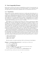
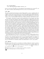
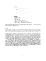
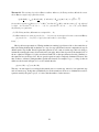
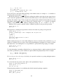
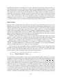
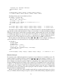
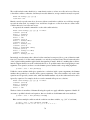
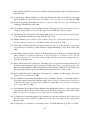
States and transition function (graphical representation to the right):
Q = {q s , qh , q1 , q2 }
M(q s , 0) = (q1 , →)
M(q s , 1) = anything
M(q1 , 0) = (q2 , 1)
M(q1 , 1) = (q1 , →)
M(q2 , 0) = (qh , 0)
M(q2 , 1) = (q2 , ←)
1/→
/ qs
0/→
/ q1
1/←
0/1
/ q2
0/0
/ qh
/
Sample computation:
(q s , 0ω 01110ω ) →M (q1 , 0ω 1110ω ) →M (q1 , 0ω 1110ω ) →M (q1 , 0ω 1110ω ) →M
(q1 , 0ω 11100ω ) →M (q2 , 0ω 11110ω ) →M (q2 , 0ω 11110ω ) →M (q2 , 0ω 11110ω ) →M
(q2 , 0ω 11110ω ) →M (q2 , 0ω 011110ω ) →M (qh , 0ω 011110ω )
Figure 2.1: Turing machine M computing the successor function, and sample computation
to functions that take any natural numbers as input and produce any natural numbers as output. For example,
Figure 2.1 shows a Turing machine computing the successor function. Cells containing 0 can then be used as
number separators, when more natural numbers are needed. For example, a Turing machine computing a
binary operation on natural numbers would run on configurations (q s , 0ω 01m+1 01n+1 0ω ) and would halt on
configurations (qh , 0ω 01k+1 0ω ), where m, n, k are natural numbers.
One can similarly have tape encodings of rational numbers; for example, one can encode the number m/n
as m followed by n with two 0 cells in-between (and keep the one-0-cell-convention for argument separation).
Real numbers are not obviously representable, though. A Turing machine is said to compute a real number r
iff it can finitely approximate r (for example using a rational number) with any desired precision; one way to
formalize this is as follows: Turing machine Mr computes r iff when run on input natural number p, it halts
with result rational number m/n such that |r − m/n| < 1/10 p . If a real number
√ can be computed by a Turing
machine then it is called Turing computable. Many real numbers, e.g., π, e, 2, etc., are Turing computable.
2.2.2
Universal Machines, the Halting Problem, and Decision Problems
Since Turing machines have finite descriptions, they can be encoded themselves as natural numbers. Therefore,
we can refer to “the kth Turing machine”, where k is a natural number, the same way we can refer to the
ith input to a Turing machine. A universal Turing machine is a Turing machine that can simulate an
arbitrary Turing machine on arbitrary input. The universal machine essentially achieves this by reading
both the description of the machine to be simulated as well as the input thereof from its own tape. There
are various constructions of universal Turing machines in the literature, which we do not repeat here. We
only notice that we can construct such a universal machine U which terminates precisely on all inputs of
the form 1k 01i where Turing machine k terminates on input i. This immediately implies that the language
{1k 01i | Turing machine k terminates on input i} is recursively enumerable. However, the undecidability of
the famous halting problem (does a given Turing machine terminates on a given input?) implies that this
language is not recursive; more specifically, it is not co-recursively enumerable.
Since the elements of many mathematical domains can be encoded as words in B? , the terminology in
Definition 8 is also used for decision problems over such domains. For example, the decision problem of
23
whether a graph given as input has a cycle or not is recursive; in other words, the set of cyclic graphs (under
some appropriate encoding in B? ) is recursive/decidable. Since there is a bijective correspondence between
elements in B? and natural numbers, and also between tuples of natural numbers and natural numbers,
decision problems are often regarded as one- or multi-argument relations or predicates over natural numbers.
For example, a subset R ⊆ B? can be regarded as a predicate, say of three natural number arguments, where
R(i, j, k) for i, j, k ∈ Nat indicates that the encoding of (i, j, k) belongs to R.
While the haling problem is typically an excellent vehicle to formally state and prove that certain
problems are undecidable, so they cannot be solved by computers no matter how powerful they are or what
programming languages are used, its reflective nature makes the halting problem sometimes hard to use in
practice. The Post correspondence problem (PCP) is an another canonical undecidable problem, which is
sometimes easier to use to show that other problems are undecidable. The PCP can be stated as follows:
given a set of (domino-style) tiles each containing a top and a bottom string of 0/1 bits, is it possible to find a
sequence of possibly repeating such tiles so that the concatenated top strings equal the concatenated bottom
strings? For example, if the given tiles are the following:
1:
◦
•◦◦
2:
◦•
◦◦
3:
••◦
••
then the answer to the PCP problem is positive, because the sequence of tiles 3 2 3 1 yields the same
concatenated strings at the top and at the bottom.
2.2.3
The Arithmetic Hierarchy
The arithmetical hierarchy defines classes of problems of increasing difficulty, called degrees, as follows:
Σ00 = Π00 = {R | R recursive}
Σ0n+1 = {P | ∃Q ∈ Π0n , ∀i(P(i) ↔ ∃ jQ(i, j))}
Π0n+1 = {P | ∃Q ∈ Σ0n , ∀i(P(i) ↔ ∀ jQ(i, j))}
For example, the Σ01 degree consists of the predicates P over natural numbers for which there is some recursive
predicate R such that for any i ∈ Nat, P(i) holds iff R(i, j) holds for some j ∈ Nat. It can be shown that Σ01
contains precisely the recursively enumerable predicates. Similarly, Π01 consists of the predicates P for which
there is some recursive predicate R such that for any i ∈ Nat, P(i) holds iff R(i, j) holds for all j ∈ Nat, which
is precisely the set of co-recursively enumerable predicates. An important degree is also Π02 , which consists
of the predicates P over natural numbers for which there is some recursive predicate R such that for any
i ∈ Nat, P(i) holds iff for any j ∈ Nat there is some k ∈ Nat such that R(i, j, k) holds. A prototypical Π02
problem is the following: giving a Turing machine M, does it terminate on all inputs? The complexity of the
problem stays in the fact that there are infinitely many (but enumerable) inputs, so one can never be “done”
with testing them; moreover, even for a given input, one does not know when to stop running the machine
and reject the input. However, if one is given for each input accepted by the machine a run of the machine,
then one can simply check the run and declare the input indeed accepted. Therefore, M terminates on all
inputs iff for any input there exists some accepting run of M, which makes it a Π02 problem because checking
whether a given run on a given Turing machine with a given input accepts the input is decidable. Moreover, it
can be shown that if we pick M to be the universal Turing machine U discussed above, then the following
problem, which we refer to as Totality from here on, is in fact Π02 -complete:
24
Input: A natural number k;
Output: Does U terminate on all inputs 1k 01i for all i ≥ 0?
For any n, both degrees Σ0n and Π0n are properly included in both the immediately above degrees Σ0n+1 and
Π0n+1 . There are extensions which define degrees Σ1n , Π2n , etc., but we do not discuss them here.
2.2.4
Notes
The abstract computational model that we call the “Turing machine” today was originally called “the
computer” when proposed by Alan Turing in 1936-37 [80]. In the original article, Turing imagined not a
machine, but a person (the computer) who executes a series of deterministic mechanical rules “in a desultory
manner”. In his 1948 essay “Intelligent Machinery”, Turing calls the machine he proposed the logical
computing machine, a name which has not been adopted, everybody preferring to call it the Turing machine.
It is insightful to understand the scientific context in which Turing proposed his machine. In the 1930s,
there were several approaches attempting to address Hilbert’s tenth question of 1900, the Entscheidungsproblem (the decision problem). Partial answers have been given by Kurt Gödel in 1930 (and published in 1931),
under the form of his famous incompleteness theorems, and in 1934, under the form of his recursion theory.
Alonzo Church is given the credit for being the first to effectively show that the Entscheidungsproblem was
indeed undecidable, introducing also λ-calculus (discussed in Section 4.5). Church published his paper on 15
April 1936, about one month before Turing submitted his paper on 28 May 1936. In his paper, Turing also
proved the equivalence of his machine to Church’s λ-calculus. Interestingly, Turing’s paper was submitted
only a few months before Emil Post, another great logician, submitted a paper independently proposing an
almost identical computational model on 7 October 1936 [62]. The major difference between Turing’s and
Post’s machines is that the former uses a tape which is infinite in only one direction, while the latter works
with a tape which is infinite at both ends, like the “Turing machine” that we used in this section. We actually
took our definitions in this section from Rogers’ book [67], which we recommend the reader for more details
in addition to comprehensive textbooks such as Sipser [76] and Hopcroft, Motwani and Ullman [33]. To
remember the fact that Post and Turing independently invented an almost identical computational model of
utmost importance, several computer scientists call it the “Post-Turing machine”.
Even though Turing was not the first to propose what we call today a Turing-complete model of
computation, many believe that his result was stronger than Church’s, in that his computational model was
more direct, easier to understand, and based on first, low-level computational principles. For example, it is
typically easy to implement Turing Machines in any programming language, which is not necessarily the case
for other Turing-complete models, such as, for example, the λ-calculus. As seen in Section 4.5, λ-calculus
relies on a non-trivial notion of substitution, which comes with the infamous variable capture problem.
2.2.5
Exercises
Exercise 12. Define Turing machines corresponding to the addition, multiplication, and power operations
on natural numbers. For example, the initial configuration of the Turing machine computing addition with
3 and 7 as input is (q s , 0ω 011110111111110ω ), and its final configuration is (qh , 0ω 0111111111110ω ). We
here assumed that n is encoded as n + 1 cells containing 1.
Exercise 13. Show that there are real numbers which are not Turing computable.
(Hint: The set of Turing machines is recursively enumerable.)
25
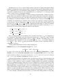
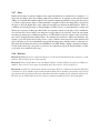
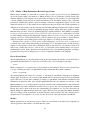
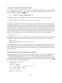
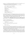
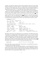
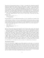
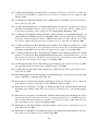
sorts:
Cell, Tape, Configuration
operations:
0, 1 : → Cell
zeros : → Tape
: : Cell × Tape → Tape
q : Tape × Tape → Configuration — one such operation for each q ∈ Q
generic equation:
zeros = 0 : zeros
specific equations:
q(L, b :R) = q0 (L, b0 :R)
— one equation for each q, q0 ∈ Q, b, b0 ∈ Cell with M(q, b) = (q0 , b0 )
0
q(L, b :R) = q (b :L, R)
— one equation for each q, q0 ∈ Q, b ∈ Cell with M(q, b) = (q0 , →)
q(B :L, b :R) = q0 (L, B : b :R) — one equation for each q, q0 ∈ Q, b ∈ Cell with M(q, b) = (q0 , ←)
lazy
Figure 2.2: Lazy equational logic representation EM of Turing machine M
2.4.3
Computation as Equational Deduction
Here we discuss simple equational logic encodings of Turing machines (see Section 2.2.1 for general Turing
machine notions). The idea is to associate an equational theory to any Turing machine, so that an input is
accepted by the Turing machine if and only if an equation corresponding to that input can be proved from
the equational theory of the Turing machine, using conventional equational deduction. Moreover, as seen in
Section 2.5.3, the resulting equational theories can be executed as rewrite theories by rewrite engines, thus
yielding actual Turing machine interpreters. We present two encodings, both based on intuitions from lazy
data-structures, specifically stream data-structures. The first is simpler but requires lazy rewriting support
from rewrite engines in order to be executed, while the second can be executed by any rewrite engines.
Lazy Equational Representation
Our first representation of Turing machines in equational logic is based on the idea that the infinite tape
can be finitely represented by means of self-expanding stream data-structures. In spite of being infinite
sequences of cells, like the Turing machine tapes, many interesting streams can be finitely specified using
equations. For example, the stream of zeros, zeros = 0 : 0 : 0 : · · · , can be defined as zeros = 0 : zeros.
Since at any given moment the portions of a Turing machine tape to the left and to the right of the head
have a suffix consisting of an infinite sequence of 0 cells, it is natural to represent them as streams of the
form b1 :b2 : · · · bn :zeros. When the head is on cell bn and the command is to move the head to the right, the
self-expanding equational definition of zeros can produce one more 0, so that the head can move onto it.
To expand zeros on a by-need basis and thus to avoid undesired non-termination due to the uncontrolled
application of the self-expanding equation of zeros, this approach requires an equational/rewrite engine with
support for lazy evaluation/rewriting in order to be executed.
Figure 2.2 shows how a Turing machine M = (Q, B, q s , qh , C, M) can be associated a computationally
lazy
equivalent equational logic theory EM . Except for the self-expanding equation of the zeros stream and our
lazy
stream representation of the two-infinite-end tape, the equations of EM are identical to the transition relation
on Turing machine configurations discussed right after Definition 7. The self-expanding equation of zeros
32
guarantees that enough 0’s can be provided when the head reaches one or the other end of the sequence of
lazy
cells visited so far. The result below shows that EM is proof-theoretically equivalent to M:
Theorem 7. The following are equivalent:
(1) The Turing machine M terminates on input b1 b2 . . . bn ;
lazy
(2) EM |= q s (zeros, b1 : b2 : · · · : bn :zeros) = qh (l, r) for some terms l, r of sort Tape.
Proof. . . .
lazy
lazy
The equations in EM can be applied in any direction, so an equational proof of EM |= q s (zeros, b1 : b2 :
· · · : bn : zeros) = qh (l, r) needs not necessarily correspond step-for-step to the computation of M on input
b1 b2 . . . bn . We will see in Section 2.5.3 that by orienting the specific equations in Figure 2.2 into rewrite
rules, we will obtain a rewrite logic theory which will faithfully capture, step-for-step, the computational
granularity of M.
Note that in Figure 2.2 we preferred to define a configuration construct q : Tape × Tape → Configuration
for each q ∈ Q. A natural alternative could have been to define an additional sort State for the Turing
machine states, a constant q : → State for each q ∈ Q, and one generic configuration construct ( , ) :
State × Tape × Tape → Configuration, as we do in the subsequent representation of Turing machines as
rewriting logic theories (see Figure 2.3). The reason for which we did not do that here is twofold: first,
in functional languages like Haskell it is very natural to associate a function to each such configuration
construct q : Tape × Tape → Configuration, while it would take some additional effort to implement the
second approach; second, the approach in this section is more compact than the one below.
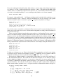
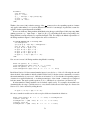
Unrestricted Equational Representation
The equational representation of Turing machines above is almost as simple as it can be and, additionally, can
be easily executed on programming languages or rewrite engines with support for lazy evaluation/rewriting,
such as Haskell or Maude (see, e.g., Section 2.5.6). However, the fact that it requires lazy evaluation/rewriting
and that the equivalence classes of configurations have infinitely many terms, its use is limited to systems that
support strategies. Here we show that a simple idea can turn the representation in the previous section into an
elementary one which can be executed on any equational/rewrite engines: replace the self-expanding and
non-terminating (when regarded as a rewrite rule) equation “zeros = 0:zeros” with configuration equations of
the form “q(zeros, R) = q(0:zeros, R)” and “q(L, zeros) = q(L, 0:zeros)”; these equations achieve the same
role of expanding zeros by need, but avoid non-termination when applied as rewrite rules.
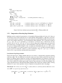
Figure 2.3 shows our unrestricted representation of Turing machines as equational logic theories. There
are some minor differences between the representation in Figure 2.3 and the one in Figure 2.2. For example,
note that in order to add the two equations above for the expanding of zeros in a generic manner for any
state, we separate the states from the configuration construct. In other words, instead of having an operation
q : Tape × Tape → Configuration for each q ∈ Q like in Figure 2.2, we now have one additional sort State, a
generic configuration construct ( , ) : State × Tape × Tape → Configuration, and a constant q : → State for
each q ∈ Q. This change still allows us to write configurations as terms q(l, r), so we do not need to change
the equations corresponding to the Turing machine transitions. With this modification in the signature, we
can now remove the troubling equation zeros = 0:zeros from the representation in Figure 2.2 and replace it
with the two safe equations in Figure 2.3. Let EM be the equational logic theory in Figure 2.3.
Theorem 8. The following are equivalent:
33
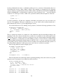
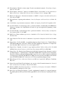
sorts:
Cell, Tape, State, Configuration
operations:
0, 1 : → Cell
zeros : → Tape
: : Cell × Tape → Tape
( , ) : State × Tape × Tape → Configuration
q : → State
— one such constant for each q ∈ Q
generic equations:
S (zeros, R) = S (0:zeros, R)
S (L, zeros) = S (L, 0:zeros)
specific equations:
q(L, b :R) = q0 (L, b0 :R)
— one equation for each q, q0 ∈ Q, b, b0 ∈ Cell with M(q, b) = (q0 , b0 )
0
q(L, b :R) = q (b :L, R)
— one equation for each q, q0 ∈ Q, b ∈ Cell with M(q, b) = (q0 , →)
0
q(B :L, b :R) = q (L, B : b :R) — one equations for each q, q0 ∈ Q, b ∈ Cell with M(q, b) = (q0 , ←)
Figure 2.3: Unrestricted equational logic representation EM of Turing machine M
(1) The Turing machine M terminates on input b1 b2 . . . bn ;
(2) EM |= q s (zeros, b1 : b2 : · · · : bn :zeros) = qh (l, r) for some terms l, r of sort Tape.
Proof. . . .
One could argue that deduction with the equational theory in Figure 2.3 is not fully faithful to computations
with the original Turing machine, because the two generic equations may need to artificially apply from time
to time as an artifact of our representation, and their application does not correspond to actual computational
steps in the Turing machine. In fact, these generic equations can be completely eliminated, at the expense of
more equations. For example, if M(q, b) = (q0 , ←) then, in addition to the last equation in Figure 2.3, we can
also include the equation:
q(zeros, b :R) = q0 (zeros, 0 : b :R)
This way, one can expand zeros and apply the transition in one equational step. Doing that systematically for
all the transitions allows us to eliminate the need for the two generic equations entirely.
34
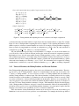
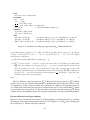
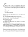
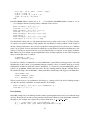
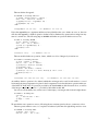
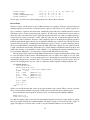
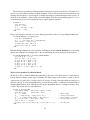
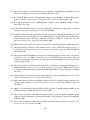
sort:
Stream
operations:
:
: Int × Stream → Stream
head : Stream → Int
tail : Stream → Stream
zeros : → Stream
zip : Stream × Stream → Stream
add : Stream → Stream
fibonacci : → Stream
equations:
head(X : S ) = X
tail(X : S ) = S
zeros = 0 : zeros
zip(X : S 1 , S 2 ) = X : zip(S 2 , S 1 )
add(X1 : X2 : S ) = (X1 +Int X2 ) : add(S )
fibonacci = 0 : 1 : add(zip(fibonacci, tail(fibonacci)))
Figure 2.8: Streams of integers defined as an algebraic datatype. The variables S , S 1 , S 2 have sort Stream
and the variables X, X1 , X2 have sort Int.
Streams
Figure 2.8 shows an example of a data-structure whose elements are infinite sequences, called streams,
together with several particular streams and operations on them. Here we prefer to be more specific than
in the previous examples and work with streams of integers. We assume the integers and operations on
them already defined; specifically, we assume Int to be their sort and operations on them indexed with Int to
distinguish them from other homonymous operations, e.g., +Int , etc. The operation : adds a given integer
to the beginning of a given stream, and the dual operations head and tail extract the head (integer) and the
tail (stream) from a stream. The stream zeros contains only 0 elements. The stream operation zip merges
two streams by interleaving their elements, and add generates a new stream by adding any two consecutive
elements of a given stream. The stream fibonacci consists of the Fibonacci sequence (see Exercise 25).
It is interesting to note that the equational specification of streams in Figure 2.8 is one where its
initial algebra semantics is likely not the model that we want. Indeed, the initial algebra here would
consists of infinite classes of finite terms, where any two terms in any class are provably equal, for example
{zeros, 0 : zeros, 0 : 0 : zeros, . . . }. While this is a valid and interesting model of streams, it is likely not
what one has in mind when one thinks of streams as infinite sequences. Nevertheless, the intended stream
model is among the models/algebras of this equational specification, so any equational deduction or reduction
that we perform, with or without strategies, is sound (see Exercise 26).
47
2.4.7
Notes
Equational encodings of general computation into equational deduction are well-known; for example, [7, 1]
show such encodings, where the resulting equational specifications, if regarded as term rewrite systems
(TRSs), are confluent and terminate whenever the original computation terminates. Our goal in this section
is to discuss equational encodings of (Turing machine) computation. These encodings will be used later in
the paper to show the Π02 -hardness of the equational satisfaction problem in the initial algebra. While we
could have used existing encodings of Turing machines as TRSs, however, we found them more complex and
intricate for our purpose in this paper than needed. Consequently (and also for the sake of self-containment),
we recall the more recent (simple) encoding and corresponding proofs from [65]. Since the subsequent
encoding is general purpose rather than specific to our Π02 -hardness result, the content of this section may
have a more pedagogical than technical nature. For example, the references to TRSs are technically only
needed to prove the equational encoding correct, so they could have been removed from the main text and
added only in the proofs, but we find them pedagogically interesting and potentially useful for other purposes.
The equational encodings that follow can be faithfully used as TRS Turing-complete computational engines,
because each rewrite step corresponds to precisely one computation step in the Turing machine; in other
words, there are no artificial rewrite steps.
2.4.8
Exercises
Exercise 24. Eliminate the two equations in Figure 2.3 as discussed right after Theorem 8, and prove a result
similar to Theorem 8 for the new representation.
Exercise 25. Show that the fibonacci stream defined in Figure 2.8 indeed defines the sequence of Fibonacci
numbers. This exercise has two parts: first formally state what to prove, and second prove it.
Exercise 26. Consider the equational specification of streams in Figure 2.8. Define the intended model/algebra
of streams over integer numbers with constant streams and functions on streams corresponding to the various
operations in this specification. Then show that this model indeed satisfies all the equations in Figure 2.8.
Describe also its default initial model and compare it with the intended model. Are they isomorphic?
48
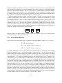
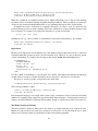
sorts:
Cell, Tape, Configuration
operations:
0, 1 : → Cell
zeros : → Tape
: : Cell × Tape → Tape
q : Tape × Tape → Configuration — one such operation for each q ∈ Q
equations:
zeros = 0 : zeros
rules:
q(L, b :R) → q0 (L, b0 :R)
— one rule for each q, q0 ∈ Q, b, b0 ∈ Cell with (q0 , b0 ) ∈ M(q, b)
0
q(L, b :R) → q (b :L, R)
— one rule for each q, q0 ∈ Q, b ∈ Cell with (q0 , →) ∈ M(q, b)
q(B :L, b :R) → q0 (L, B : b :R) — one rule for each q, q0 ∈ Q, b ∈ Cell with (q0 , ←) ∈ M(q, b)
lazy
Figure 2.10: Lazy rewriting logic representation RM of Turing machine M
2.5.3
Computation as Rewriting Logic Deduction
Building upon the equational representations of deterministic Turing machines in Section 2.4.3, here we
show how we can associate rewrite theories to non-deterministic Turing machines so that there is a bijective
correspondence between computational steps performed by the original Turing machine and rewrite steps
in the corresponding rewrite theory. In non-deterministic Turing machines, the total transition function
M : (Q − {qh }) × B → Q × C generalizes to a total relation, or in other words to a function into the strict
powerset of Q × C, M : (Q − {qh }) × B → P+ (Q × C), that is, taking each non-halting state q and current cell
bit contents b into a non-empty set M(q, b) of non-deterministic (state,action) choices. For example, to turn
the successor Turing machine in Figure 2.1 into one which non-deterministically chooses to add one more
1 to the given number or not when it reaches its end, all we have to do is to modify its transition function
in state q1 and cell contents 0 to return two possible continuations: M(q1 , 0) = {(q2 , 1), (q2 , ←)}. Like in
Section 2.4.3, we give both lazy and unrestricted representations.
Lazy Rewrite Logic Representation
Figure 2.10 shows how a Turing machine M can be associated a computationally equivalent rewriting
lazy
logic theory RM . The only difference between this rewrite logic theory and the equational logic theory in
Figure 2.2 is that the equations which were specific to the Turing machine have been turned into rewrite rules.
The equation expanding the stream of zeros remains an equation. Since in rewriting logic only the rewrite
rules count as transitions, and they apply modulo equations, the rewrite theory is in fact more faithful to the
actual computational steps embodied in the Turing machine. The result below formalizes this by showing
lazy
that there is a step-for-step equivalence between computations using M and rewrites using RM :
lazy
Theorem 10. The rewriting logic theory RM is confluent. Moreover, the Turing machine M and the rewrite
lazy
theory RM are step-for-step equivalent, that is,
−
→
−
lazy
−v ) →1 q0 (←
(q, 0ω ubv0ω ) →M (q0 , 0ω u0 b0 v0 0ω ) if and only if RM |= q(←
u−, b : →
u0 , b0 : v0 )
57
sorts:
Cell, Tape, State, Configuration
operations:
0, 1 : → Cell
zeros : → Tape
: : Cell × Tape → Tape
( , ) : State × Tape × Tape → Configuration
q : → State
— one such constant for each q ∈ Q
equations:
S (zeros, R) = S (0:zeros, R)
S (L, zeros) = S (L, 0:zeros)
rules:
q(L, b :R) → q0 (L, b0 :R)
— one rule for each q, q0 ∈ Q, b, b0 ∈ Cell with (q0 , b0 ) ∈ M(q, b)
0
q(L, b :R) → q (b :L, R)
— one rule for each q, q0 ∈ Q, b ∈ Cell with (q0 , →) ∈ M(q, b)
0
q(B :L, b :R) → q (L, B : b :R) — one rule for each q, q0 ∈ Q, b ∈ Cell with (q0 , ←) ∈ M(q, b)
Figure 2.11: Unrestricted rewriting logic representation RM of Turing machine M
for any finite sequences of bits u, v, u0 , v0 ∈ {0, 1}∗ , any bits b, b0 ∈ {0, 1}, and any states q, q0 ∈ Q, where if
−u = b : b : · · · : b
u = b1 b2 . . . bn−1 bn , then ←
u− = bn : bn−1 : · · · : b2 : b1 : zeros and →
1
2
n−1 : bn : zeros. Finally,
the following are equivalent:
(1) The Turing machine M terminates on input b1 b2 . . . bn ;
lazy
(2) RM |= q s (zeros, b1 : b2 : · · · : bn :zeros) → qh (l, r) for some terms l, r of sort Tape; note though that
lazy
RM does not terminate on term q s (zeros, b1 : b2 : · · · : bn :zeros) as an unrestricted rewrite system,
since the equation zeros = 0 : zeros (regarded as a rewrite rule) can apply forever, thus yieldlazy
ing infinite equational classes of configurations with no canonical forms, but RM terminates on
q s (zeros, b1 : b2 : · · · : bn :zeros) if the stream construct operation : : Cell × Tape → Tape has a lazy
rewriting strategy on its second argument;
Proof. . . .
lazy
lazy
Therefore, unlike the equational logic theory EM in Theorem 7, the rewrite logic theory RM faithfully
captures, step-for-step, the computational granularity of M. Recall that equational deduction does not count
as computational, or rewrite steps in rewriting logic, which allows to apply the self-expanding equation of
zeros silently in the background. Since there are no artificial rewrite steps, we can conclude that RM actually
is precisely M and not an encoding of it. Theorem 10 thus showed not only that rewriting logic is Turing
complete, but also that it faithfully captures the computational granularity of the represented Turing machines.
Unrestricted Rewrite Logic Representations
Figure 2.11 shows our unrestricted representation of Turing machines as rewriting logic theories, following
the same idea as the equational representation in Section 2.4.3 (Figure 2.3). Let RM be the rewriting logic
theory in Figure 2.11. Then the following result holds:
58
Theorem 11. The rewriting logic theory RM is confluent. Moreover, the Turing machine M and the rewrite
theory RM are step-for-step equivalent, that is,
(q, 0ω ubv0ω ) →M (q0 , 0ω u0 b0 v0 0ω ) if and only if
−
→
−
−v ) →1 q0 (←
RM |= q(←
u−, b : →
u0 , b0 : v0 )
for any finite sequences of bits u, v, u0 , v0 ∈ {0, 1}∗ , any bits b, b0 ∈ {0, 1}, and any states q, q0 ∈ Q, where if
−u = b : b : · · · : b
u− = bn : bn−1 : · · · : b2 : b1 : zeros and →
u = b1 b2 . . . bn−1 bn , then ←
1
2
n−1 : bn : zeros. Finally,
the following are equivalent:
(1) The Turing machine M terminates on input b1 b2 . . . bn ;
(2) RM terminates on term q s (zeros, b1 : b2 : · · · : bn :zeros) as an unrestricted rewrite system and RM |=
q s (zeros, b1 : b2 : · · · : bn :zeros) → qh (l, r) for some terms l, r of sort Tape;
Proof. . . .
Like for the lazy representation of Turing machines in rewriting logic discussed above, the rewrite theory
RM is the Turing machine M, in that there is a step-for-step equivalence between computational steps in
M and rewrite steps in RM . Recall, again, that equations do not count as rewrite steps, their role being to
structurally rearrange the term so that rewrite rules can apply; indeed, that is precisely the intended role of
the two equations in Figure 2.11 (they reveal new blank cells on the tape whenever needed). Similarly to
the equational case in Section 2.4.3, the two generic equations can be completely eliminated. However, this
time we have to add more Turing-machine-specific rules instead. For example, if (q0 , ←) ∈ M(q, b) then, in
addition to the last rule in Figure 2.11, we also include the rule:
q(zeros, b :R) → q0 (zeros, 0 : b :R)
This way, one can expand zeros and apply the transition in one rewrite step, instead of one equational step
and one rewrite step. Doing that systematically for all the transitions allows us to eliminate the need for
equations entirely; the price to pay is, of course, that the number of rules increases.
59
2.5.6
Maude: A High Performance Rewrite Logic System
Maude (http://maude.cs.uiuc.edu) is a rewrite logic executable specification language, which builds
upon a fast rewrite engine. Our main use of Maude in this book is as a platform to execute rewrite logic
semantic definitions, following the various approaches in Chapter 3. Our goal here is to give a high-level
overview of Maude, mentioning only its features needed in this book. We make no attempt to give a systematic
presentation of Maude here, meant to replace its manual or other more comprehensive papers or books (some
mentioned in Section 2.5.8). The features we need will be introduced on-the-fly, with enough explanations to
make this book self-contained, but the reader interested in learning Maude in depth should consult its manual.
We will use Maude to specify programming language features, which, when put together via simple
Maude module operations, lead to programming language semantic definitions. Since Maude is executable,
interpreters for programming languages designed this way will be obtained for free, which will be very useful
for understanding, refining and/or changing the languages. Moreover, formal analysis tools for the specified
languages can also be obtained with little effort, such as exhaustive state-space searchers or model-checkers,
simply by using the corresponding generic rewrite logic analysis tools already provided by Maude.
Devising formal semantic executable models of desired languages or tools before these are implemented
is a crucial step towards a deep understanding of the language or tool. In simplistic terms, it is like devising a
simulator for an expensive system before building the actual system. However, our simulators in this book
will consist of exactly the semantics, or the meaning, of our desired systems, defined using a very rigorous,
mathematical notation. In the obtained formal executable model of a programming language, executing a
program will correspond to nothing but logical inference within the semantics of the language.
How to Execute Maude
After installing Maude on your platform and setting up the environment path variable, you should be able to
type maude and immediately see a welcome screen followed by a cursor waiting for user input:
Maude>
Maude is interpreted, so you can just type your specifications and commands. However, a more practical way
is to type everything in one file, say pgm.maude, and then include that file with the command
Maude> in pgm.maude
after starting Maude (the extension is optional), or, alternatively, start Maude with pgm as an argument:
“maude pgm”. In both cases, the contents of pgm.maude will be loaded and executed as if it was manually
typed at the cursor. Use the quit command, or simply q, to quit Maude. Since Maude’s initialization and
termination are quite fast, many users end their pgm.maude file with a q command on a new line, so that
Maude terminates as soon as the program is executed. Another useful command in files is eof, which tells
Maude that the end-of-file is meant there and thus it does not process the code following the eof command.
Instead, the control is given to the user, who can manually type commands, etc. You can correct/edit your
Maude definition in pgm.maude and then load it again. However, keep it in mind that Maude maintains
only one working session, in particular one module database, until you quit it. This can sometimes lead to
unexpected errors for beginners, so if you are not sure about an error just quit and then restart Maude.
Modules
Maude specifications are introduced as modules. There are several kinds of modules, but for simplicity we
only use general modules in this book, which have the syntax
61
mod <NAME> is
<BODY>
endm
where <NAME> can be any identifier. The <BODY> of a module can include importation of other modules, sort
and operation declarations, and a set of sentences. The sorts together with the operations form the signature
of that module, and can be thought of as the interface of that module to other modules.
To lay the ground for introducing more Maude features, let us define Peano-style natural numbers with
addition and multiplication. We define the addition first, in one separate module:
mod PEANO-NAT is
sort Nat .
op zero : -> Nat .
op succ : Nat -> Nat .
op plus : Nat Nat -> Nat .
vars N M : Nat .
eq plus(zero, M) = M .
eq plus(succ(N), M) = succ(plus(N, M)) .
endm
Declarations and sentences are always terminated by periods, which should have white spaces before and
after. Forgetting a terminal period or a white space before the period are two of the most common errors that
Maude beginners make.
The signature of PEANO-NAT consists of one sort, Nat, and three operations, namely zero, succ, and
plus. Sorts are declared with the keywords sort or sorts, and operations with op or ops.
The three operations have zero, one and two arguments, respectively, whose sorts are listed between the
symbols : and ->. Operations of zero arguments are also called constants, those of one argument are called
unary and those of two binary. The result sort appears right after the symbol ->.
We use ops when two or more operations of same arguments are declared together, to save space, and
then we use white spaces to separate them:
ops plus mult : Nat Nat -> Nat .
There are few special characters in Maude, and users are allowed to define almost any token or combination
of tokens as operation names. If you use op in the above instead of ops, for example, then only one operation,
called “plus mult”, is declared.
The two equations in PEANO-NAT are properties, or constraints, that terms built with these operations
must satisfy. Another way to look at equations is through the lenses of possible implementations of the
specifications they define; in our case, any correct implementation of Peano natural numbers should satisfy the
two equations. Equations are quantified universally with the variables they contain, and can be applied from
left-to-right or from right-to-left in reasoning, which means that equational proofs may require exponential
search, thus making them theoretically intractable. Maude provides limited support for equational reasoning.
reduce: Rewriting with Equations
When executing specifications, Maude regards all equations as rewrite rules, which means that they are
applied only from left to right. Moreover, they are applied iteratively for as long as their left-hand-side terms
match any subterm of the term to reduce. This way, any well-formed term can either be derived infinitely
often, or be reduced to a normal form, which cannot be reduced anymore by applying equations as rewriting
rules. Maude’s command to reduce a term to its normal form using equations as rewrite rules is reduce, or
simply red. Reduction will be made in the last defined module, which is PEANO-NAT in our case:
62
Maude> reduce plus(plus(succ(zero),succ(succ(zero))), succ(succ(succ(zero)))) .
rewrites: 6 in 0ms cpu (0ms real) (˜ rewrites/second)
result Nat: succ(succ(succ(succ(succ(succ(zero))))))
Make sure commands are terminated with a period. Maude implements state of the art term rewriting
algorithms, based on advanced indexing and pattern matching techniques. This way millions of rewrites per
second can be performed, making Maude usable as a programming language in terms of performance.
Sometimes the results of reductions are repetitive and may be too large to read. To ameliorate this
problem, Maude provides an operator attribute called iter, which allows to input and print repetitive terms
more compactly. For example, if we replace the declaration of operation succ with
op succ : Nat -> Nat
[iter] .
then Maude uses, e.g., succˆ3(zero) as a shorthand for succ(succ(succ(zero))). For example,
Maude> reduce plus(plus(succ(zero),succˆ2(zero)), succˆ3(zero)) .
result Nat: succˆ6(zero)
Importation
Modules can be imported in several different ways. The difference between importation modes is subtle and
semantical rather than operational, and it is not relevant in this book. Therefore, we only use the most general
of them, including. For example, the following module extends PEANO-NAT with multiplication:
mod PEANO-NAT* is
including PEANO-NAT .
op mult : Nat Nat -> Nat .
vars M N : Nat .
eq mult(zero, M) = zero .
eq mult(succ(N), M) = plus(mult(N, M), M) .
endm
It is safe to think of including as “copy and paste” the contents of the imported module into the importing
module, with one exception: variable declarations are not imported, so they need to be redeclared.
We can now “execute programs” using features in both modules:
red mult(plus(succ(zero),succ(succ(zero))), succ(succ(succ(zero)))) .
The following is Maude’s output:
rewrites: 18 in 0ms cpu (0ms real) (˜ rewrites/second)
result Nat: succˆ9(zero)
Even though this language is very simple and its syntax is ugly, it nevertheless shows a formal and executable
definition of a language using equational logic and rewriting. Other languages or formal analyzers discussed
in this book will be defined in a relatively similar manner, though, as expected, they will be more involved.
The Mixfix Notation and Parsing
The plus and mult operations defined above are meant to be written using the prefix notation in terms.
Maude also supports the mixfix notation for operations (see Section 2.1.3), by allowing the user to write
underscores in operation names as placeholders for their corresponding arguments.
63
op
op
op
op
_+_ : Int Int -> Int .
_! : Nat -> Nat .
in_then_else_ : BoolExp Stmt Stmt -> Stmt .
_?_:_ : BoolExp Exp Exp -> Exp .
Users can now also write terms taking advantage of the mixfix notation, for example 3 + 5, in addition to
the usual prefix notation, that is, + (3,5).
Recall from Section 2.1.3 that, syntactically speaking, the mixfix notation has the same expressiveness
as the context-free grammar notation. Therefore, the mixfix notation comes with the unavoidable parsing
problem. For example, suppose that we replace the operations plus and mult in the modules above with
their mixfix variants + and * (see also Exercise 29). Then the term X + Y * Z, with X, Y, Z arbitrary
variables (or any terms) of sort Nat, admits two ambiguous parsings: (X + Y) * Z and X + (Y * Z).
Maude provides a parse command, similar to reduce except that it only parses the given term:
Maude> parse X + Y .
Nat: X + Y
Maude generates a warning message whenever it detects more than one parsing of the given term:
Maude> parse X + Y * Z .
Warning: <standard input>, line 1: ambiguous term, two parses are:
X + (Y * Z)
-versus(X + Y) * Z
Arbitrarily taking the first as correct.
Nat: X + (Y * Z)
Similar warning messages are issued when ambiguous terms are detected in the specification (e.g., in
equations). In general, we do not want to allow any parsing ambiguity in specifications or in terms to rewrite.
One simple way to avoid ambiguities is to use parentheses to specify the desired grouping, for example:
Maude> parse X + (Y * Z) .
Nat: X + (Y * Z)
To reduce the number of parentheses, Maude allows us to assign precedences to mixfix operations declared in
its modules, specifically as operator attributes in square brackets using the prec keyword. For example:
op _+_ : Nat Nat -> Nat [prec 33] .
op _*_ : Nat Nat -> Nat [prec 31] .
The lower the precedence the stronger the binding! As expected, now there is no parsing ambiguity anymore:
Maude> parse X + Y * Z .
Nat: X + Y * Z
To see how the term was parsed, set the “print with parentheses” flag on:
Maude> set print with parentheses on .
Maude> parse X + Y * Z .
Nat: (X + (Y * Z))
If displaying the parentheses is not sufficient, then disable the mixfix printing completely:
Maude> set print mixfix off .
Maude> parse X + Y * Z .
Nat: _+_(X, _*_(Y, Z))
64
Associativity, Commutativity and Identity Attributes
Some of the binary operations used in this book will be associative (A), commutative (C) or have an identity
(I), or combinations of these. E.g., + is associative, commutative and has 0 as identity. All these can be
added as attributes to operations when declared:
op _+_ : Int Int -> Int [assoc comm id: 0 prec 33] .
op _*_ : Int Int -> Int [assoc comm id: 1 prec 31] .
Note that each of the A, C, and I attributes are logically equivalent to appropriate equations, such as
eq A + (B + C) = (A + B) + C .
eq A + B = B + A . ---> attention: rewriting does not terminate!
eq A + 0 = A .
When applied as rewrite rules, each of the three equations above have limitations. The associativity equation
forces all the parentheses to be grouped to the left, which may prevent some other rules from applying. The
commutativity equation may lead to non-termination when applied as a rewrite rule. The identity equation
would only be able to simplify expressions, but not to add a 0 to an expression, which may be useful in
some situations (we will see such situations shortly, in the context of lists). Maude’s builtin support for ACI
attributes addresses all the problems above. Additionally, the assoc attribute of a mixfix operation is also
taken into account by Maude’s parser, which hereby eliminates the need for some useless parentheses:
Maude> parse X + Y + Z .
Nat: X + Y + Z
An immediate consequence of the builtin support for the comm attribute, which allows rewriting with
commutative operations to terminate, is that normal forms will be reported now modulo commutativity:
Maude> red X + Y + X .
rewrites: 0 in 0ms cpu (0ms real) (˜ rewrites/second)
result Nat: X + X + Y
As seen, Maude picked to display some equivalent (modulo AC) of the original term (extracted from how the
current implementation of Maude stores this term internally). There were 0 rewrites applied in the reduction
above, because the internal rearrangements of terms according to the ACI attribute annotations do not count
as rule applications.
Matching Modulo Associativity, Commutativity, and Identity
Here we discuss Maude’s support for ACI matching, which is arguably one of the most distinguished and
complex Maude features, and nevertheless the reason and the most important use of the ACI attributes.
We discuss ACI matching by means of a series of examples, starting with lists, which occur in many
programming languages. The following module defines lists of integers with a membership operation in ,
based on AI (associative and identity) matching:
mod INT-LIST is including INT .
sort IntList .
subsort Int < IntList .
op nil : -> IntList .
op __ : IntList IntList -> IntList [assoc id: nil] .
op _in_ : Int IntList -> Bool .
var I : Int . vars L L’ : IntList .
eq I in L I L’ = true .
eq I in L = false [owise] .
endm
65
We start by including the builtin INT module, which declares a sort Int and provides arbitrary large integers
as constants of sort Int, together with the usual operations on these. The builtin module BOOL, which
similarly declares a sort Bool and common Boolean operations on it, is automatically included in all modules,
so it needs not be included explicitly. To see a an existing module, builtin or not, use the command
Maude> show module <NAME> .
For example, “show module INT .” will display the INT module. In the INT-LIST module above, note
the subsort declaration “Int < IntList”, which says that integers are also lists of integers. This, together
with the constant nil and the concatenation operation , can generate any finite list of integers:
Maude> parse 1 2 3 4 5 .
IntList: 1 2 3 4 5
Maude> red 1 nil 2 nil 3 nil 4 nil 5 6 7 nil .
rewrites: 0 in 0ms cpu (0ms real) (˜ rewrites/second)
result IntList: 1 2 3 4 5 6 7
Note how the reduce command above eliminated all the unnecessary nil constants from the list, in zero
rewrite steps, for the same reason as above: the internal rearrangements according to the ACI attributes do
not count as rewrite steps.
The two equations defining the membership operation make use of AI matching. The first equation says
that if we can match the integer I anywhere inside the list, then we are done. Since the list constructor was
declared associative and with identity nil, Maude is mathematically allowed to bind the variables L and L’
of sort IntList to any lists of integers, including the empty one. Maude indeed does this through its efficient
AI matching algorithm. Equations with attribute owise are applied only when other equations fail to apply.
Therefore, we defined the semantics of the membership operation only by means of AI matching, without
having to implement any explicit traversal of the list. Here are some examples testing the semantics above:
Maude>
result
Maude>
result
Maude>
result
red 3
Bool:
red 3
Bool:
red 3
Bool:
in 2 3 4 .
true
in 3 4 5 .
true
in 1 2 4 .
false
To define sets of integers (see, e.g., Exercise 30), besides likely renaming the sort IntList into IntSet,
we would also need to declare the concatenation operation commutative; moreover, thanks to Maude’s
commutative matching, we can also replace the first equation by “eq I in I L = true .”
We next discuss a Maude definition of (partial finite-domain) maps (see Section 2.4.6 and Figure 2.7
for the mathematical definition). We assume that the Source and Target sorts are defined in separate
modules SOURCE and TARGET, respectively; one may need to change these in concrete applications. The
associativity, commutativity and identity equations in Figure 2.7 are replaced by corresponding Maude
operational attributes. Note that the second equation defining the update operation takes advantage of
Maude’s owise attribute (explained above), so it departs from the more mathematical definition in Figure 2.7:
mod MAP is including SOURCE + TARGET .
sort Map .
op _|->_ : Source Target -> Map [prec 0] .
op empty : -> Map .
op _,_ : Map Map -> Map [assoc comm id: empty] .
op _(_) : Map Source -> Target [prec 0] .
--- lookup
op _[_/_] : Map Target Source -> Map [prec 0] . --- update
66
var M : Map . var A : Source . var B B’ : Target .
eq (M, A |-> B)(A) = B .
eq (M, A |-> B’)[B / A ] = (M, A |-> B) .
eq M[B / A] = (M, A |-> B) [owise] .
endm
If module SOURCE defines constants a, b, c, d, . . . , of sort Source, and TARGET defines constants 1, 2, 3, 4,
. . . , of sort Target, then the following reduce commands work as shown:
Maude>
result
Maude>
result
Maude>
result
Maude>
result
red empty[1 / a][2
Map: a |-> 1,b |->
red empty[1 / a][2
Map: a |-> 4,b |->
red empty[1 / a][2
Target: 4
red empty[1 / a][2
Target: (a |-> 4,b
/ b][3 / c] .
2,c |-> 3
/ b][3 / c][4 / a] .
2,c |-> 3
/ b][3 / c][4 / a](a) .
/ b][3 / c][4 / a](d) .
|-> 2,c |-> 3)(d)
Note that the last reduction above only updated the map, but it got stuck on the lookup of d. That is because
we only have one equation defining lookup, which works only when the looked up element is in the domain of
the map. Getting stuck terms as above may be acceptable in many applications, but, however, we sometimes
want to report specific errors in such situations. Maude has several advanced foundational mechanisms to deal
with errors, but they are non-trivial and we do not need them in this book. Instead, we can simply modify the
MAP definition above to include a special undefined “value” and then explicitly use this value in equations
where we mean that an error occurred:
op undefined : -> Map .
eq M(A) = undefined [owise] .
Now the last reduction command above yields undefined. A particularly useful approach to deal with
undefinedness in the context of programming language semantics, where a semantics builts upon several
mathematical domains in which the syntax is interpreted, is to define the constant undefined to have a
generic sort, say Domain, which is then subsorted to all sorts, including Source, Target, and Map. Then we
can add the following to the module MAP to obtain partial finite-domain maps with support for undefinedness:
subsort Domain < Map .
eq M(A) = undefined [owise] .
eq A |-> undefined = empty .
The last equation above is an optimization, allowing us to “garbage collect” the useless bindings in maps
once they are explicitly “undefined” in certain elements. For example,
Maude> red empty[1 / a][2 / b][3 / c][4 / a][undefined / a] .
result Map: b |-> 2,c |-> 3
Pretty Printing
In the MAP example above, the bindings and the comma separating them may be hard to read when the maps
are large. We may therefore want to pretty-print the reduced terms. Maude provides the format attribute for
this purpose. For example, if we replace the operation declarations of |-> and , with
op _|->_ : Source Target -> Map [prec 0 format(d b o d)] .
op _,_ : Map Map -> Map [assoc comm id: empty format(d sr! oss d)] .
67
then the former will always be displayed in color blue, while the second in bold red and preceded by one
space and followed by two spaces. Each group of characters in the argument of format refers to a pointcut
in the operation name; we have default pointcuts at the beginning and at the end of the operation name, as
well pointcuts before and after any special token (underscore, comma, and the various kinds of parentheses
and brackets). In each group of characters, d means “default” and is used alone to skip that pointcut and
move to the next, b and r the colors blue and red, o means to revert to the original color and style, s means
one space, and ! means bold font. There are also indentation attributes, which we have not used here but we
will use later in the book, such as: + and - to increment and decrement the global indent counter, respectively,
i to print the number of spaces determined by indent counter, and n to print a newline.
Built-in Modules
Maude provides several builtin modules and has been designed in a way that existing modules can be easily
changed and more modules can be added. It is likely that at this moment Maude’s builtin modules are not
identical to the homonymous ones when this book was written, and it also likely that new modules have been
added since then. To avoid depending on particular versions of Maude, and also to avoid unfortunate naming
conflicts with existing builtins which prevent us from naming programming language constructs as desired,
in this book we actually define a custom version builtins, discussed in Section A.1. Nevertheless, some of
Maude’s current builtin modules make interesting use of ACI matching and are also present in our custom
builtins, albeit using different names, so we briefly discuss them here.
As already discussed, the INT module provides a sort Int with arbitrarily large integers and common
operations on them. All these are essentially hooked to C library functions through a special interface that
Maude provides, which we do not discuss here but refer the interested reader to Section A.1 for details.
Similarly, there is a builtin module named QID, from “quoted identifiers”, which provides a sort Qid
together with arbitrary large quoted identifiers, as constants of sort Qid, such as the following: ’a, ’b,
‘abc123, ’a-larger-identifier, etc. These can be used as identifiers, e.g., as program variable names,
in the programming languages that we define and execute using Maude.
Let us next discuss the module BOOL, which by default Maude includes in every other module (there
are ways to disable the automatic inclusion, discussed in Section A.1). Besides the sort Bool with its two
Boolean constants true and false, BOOL includes three important polymorphic operations and the usual
Boolean operations. The polymorphic operations have the following syntax:
op if_then_else_fi : Bool Universal Universal -> Universal [...]
op _==_ : Universal Universal -> Bool [...]
op _=/=_ : Universal Universal -> Bool [...]
We excluded their specific attributes because they use advanced Maude features which are not necessary
anywhere else in this book. Instead, we explain their behavior in words. The builtin sort Universal can be
thought of as a generic sort, which can be instantiated with any concrete sort. Operation if then else fi is
strict in its first argument and lazy in its second and third arguments, that is, it only allows rewrites to take
place in its first argument but not in the other two arguments. If the first argument rewrites to true then the
conditional rewrites to its second argument, and if thefirst argument rewrites to false then the conditional
rewrites to its third argument. We will discuss rewrite strategies in more depth later in this section. The other
two operations correspond to operational equality and inequality of terms: the two terms are first rewritten
to their normal forms and then those are compared modulo the existing operation ACI attributes. While
operational equality implies logical equality, the other implication does not hold and tends to be a source of
confusion, sometimes even among Maude experts: two terms t and t0 may be provably equal using equational
68
reasoning, yet t == t0 may still rewrite to false. In this case, false only means that Maude was not able to
show the two terms equal by rewriting them to their normal forms.
The definitions of the usual Boolean operations make interesting use of AC matching:
op _and_ : Bool Bool -> Bool [assoc comm prec 55] .
op _or_ : Bool Bool -> Bool [assoc comm prec 59] .
op _xor_ : Bool Bool -> Bool [assoc comm prec 57] .
op not_ : Bool -> Bool [prec 53] .
op _implies_ : Bool Bool -> Bool [prec 61 gather (e E)] .
vars A B C : Bool .
eq true and A = A .
eq false and A = false .
eq A and A = A .
eq false xor A = A .
eq A xor A = false .
eq A and (B xor C) = A and B xor A and C .
eq not A = A xor true .
eq A or B = A and B xor A xor B .
eq A implies B = not (A xor A and B) .
It can be shown that the equations above, when applied as rewrite rules, yield a decision procedure for
propositional logic. Specifically, if we only consider Bool terms which are variables, any valid proposition
rewrites to true and any unsatisfiable one to false; the remaining (satisfiable but invalid) propositions are
rewritten to a canonical form consisting of an exclusive disjunction (xor) of conjunctions (and). We refer the
interested reader to Section 2.3 for terminology and basic propositional logic results.
The attribute gather(e E) of implies tells the Maude parser that we want implies to be right
associative, this way avoiding to add unnecessary parentheses in Boolean expressions. There is a similar
attribute, gather(E e), for left associativity. We do not discuss the gather attribute any further in this book.
Constructor versus Defined Operations
Recall the two equations of the module PEANO-NAT:
eq plus(zero, M) = M .
eq plus(succ(N), M) = succ(plus(N, M)) .
These equations constrain the three operations of the module, namely
op zero : -> Nat .
op succ : Nat -> Nat .
op plus : Nat Nat -> Nat .
But why did we write them in that particular style, which resembles a recursive definition of a function plus
in terms of data-type constructors zero and succ? Intuitively, that is because we want plus to be completely
defined in terms of zero and succ. Formally, this means that any term over the syntax zero, succ, and
plus can be shown, using the given equations, equal to a term containing only zero and succ operations,
that is, zero and succ alone are sufficient to build any Peano number.
While Maude at its core makes no distinction between operations meant to be data-type constructors
and operations meant to be functions, it is still meaningful to distinguish the operations of a module into
constructor and defined operations. Note, however, that it is the way we write the equations in the module,
and only that, which makes the operations become constructors or defined. If we forget an equation dealing
with a case (e.g., an intended constructor) for an operation intended to be defined, then that operation cannot
69
be always eliminated from terms, so technically speaking it is also a constructor. Unfortunately, there is no
silver-bullet recipe on how to define “defined” operators, but essentially a good methodology is to define the
operator’s behavior on each intended constructor. That is what we did when we defined plus in PEANO-NAT
and mult in PEANO-NAT*: we defined them on zero and on succ. In general, if c1, . . . , cn are the intended
constructors of a data-type, in order to define a new operation d, make sure that all equations of the form
eq d(c1(...)) = ...
...
eq d(cn(...)) = ...
are in the specification. If d has more arguments, then make sure that the above cases are listed for at
least one of its arguments. This gives no guarantee (e.g., one can “define” plus as plus(succ(M),N) =
plus(succ(M),N)), but it is a good enough principle to follow.
Let us demonstrate the above by defining several operations. Consider the following specification of lists:
mod INT-LIST is including INT .
sort IntList . subsort Int < IntList .
op __ : Int IntList -> IntList [id: nil] .
op nil : -> IntList .
endm
The two operations are meant to be constructors for lists, namely the empty list and adding an integer to the
beginning of a list. Note, however, that the above contains three constructors for lists at first sight, because
the subsorting of Int to IntList states that sole integers are also lists. Indeed, without the identity attribute
of , we would have to consider three cases when defining operations over lists. However, with the identity
declaration Maude will internally identity integers I with lists I nil, so only two constructors are needed,
corresponding to the two declared operations. Let us next define several important and useful operations on
lists. Notice that the definition of each operator treats each of the two constructors separately.
The following defines the usual list length operator:
mod LENGTH is including INT-LIST .
op length : IntList -> Nat .
var I : Int . var L : IntList .
eq length(I L) = 1 + length(L) .
eq length(nil) = 0 .
endm
red length(1 2 3 4 5) .
***> should be 5
The following defines list membership, without speculating matching (in fact, this would not be possible
anyway because concatenation is not defined associative as before):
mod IN is including INT-LIST .
op _in_ : Int IntList -> Bool .
vars I J : Int . var L : IntList .
eq I in J L = if I == J then true else I in L fi .
eq I in nil = false .
endm
red
red
red
red
3
3
3
3
in
in
in
in
2
3
1
1
3
4
2
2
4
5
3
4
.
.
.
.
***>
***>
***>
***>
should
should
should
should
be
be
be
be
true
true
true
false
70
The next defines list append:
mod APPEND is including INT-LIST .
op append : IntList IntList -> IntList .
var I : Int . vars L1 L2 : IntList .
eq append(I L1, L2) = I append(L1, L2) .
eq append(nil, L2) = L2 .
endm
red append(1 2 3 4, 5 6 7 8) .
***> should be 1 2 3 4 5 6 7 8
Notice that append has two arguments and that we have picked the first one to define our cases on. One can
still show that append is a defined operation, in that it can be eliminated by equational reasoning from any
term of sort IntList. The following imports APPEND and defines an operation which reverses a list:
mod REV is including APPEND .
op rev : IntList -> IntList .
var I : Int . var L : IntList .
eq rev(I L) = append(rev(L), I) .
eq rev(nil) = nil .
endm
red rev(1 2 3 4 5) .
***> should be 5 4 3 2 1
The next module defines an operation, isort, which sorts a list of integers by insertion sort:
mod ISORT is including INT-LIST .
op isort : IntList -> IntList .
vars I J : Int . var L : IntList .
eq isort(I L) = insert(I, isort(L)) .
eq isort(nil) = nil .
op insert : Int IntList -> IntList .
eq insert(I, J L) = if I > J then J insert(I,L) else I J L fi .
eq insert(I, nil) = I .
endm
red isort(4 7 8 1 4 6 9 4 2 8 3 2 7 9) .
***> should be 1 2 2 3 4 4 4 6 7 7 8 8 9 9
An auxiliary insert operation is also defined, which takes an integer and a sorted list and rewrites to a sorted
list inserting the integer argument at its place in the list argument. Notice that this latter operation makes use
of the builtn if then else fi operation provided by the default BOOL module discussed above, as well as
of the integer comparison operation “>” provided by the builtin module INT.
Let us now consider binary trees, where a tree is either empty or an integer with a left and a right subtree:
mod TREE is including INT .
sort Tree .
op ___ : Tree Int Tree -> Tree .
op empty : -> Tree .
endm
We next define some operations on trees, following the tree structure given by the two constructors above.
The next operation mirrors a tree, i.e., it replaces left subtrees by the mirrored right siblings and vice-versa:
mod MIRROR is including TREE .
op mirror : Tree -> Tree .
vars L R : Tree . var I : Int .
71
eq mirror(L I R) = mirror(R) I mirror(L) .
eq mirror(empty) = empty .
endm
red mirror((empty 3 (empty 1 empty)) 5 ((empty 6 empty) 2 empty)) .
***> should be (empty 2 (empty 6 empty)) 5 ((empty 1 empty) 3 empty)
Searching in binary trees can be defined as follows:
mod SEARCH is including TREE .
op search : Int Tree -> Bool .
vars I J : Int . vars L R : Tree .
eq search(I, L I R) = true .
ceq search(I, L J R) = search(I, L) or search(I, R) if I =/= J .
eq search(I, empty) = false .
endm
red search(6, (empty 3 (empty 1 empty)) 5 ((empty 6 empty) 2 empty)) .
red search(7, (empty 3 (empty 1 empty)) 5 ((empty 6 empty) 2 empty)) .
***> should be true
***> should be false
Note that we used a conditional equation above. Conditional equations are introduced with the keyword
ceq, and their condition with the keyword if. There are several types of conditions in Maude, which we
will discuss in the sequel, as needed. Here we used the simplest of them, namely a Bool term. To be faithful
to rewriting logic (Section 2.5), we can regard a Boolean condition b as syntactic sugar for the equality
b = true; in fact, Maude also allows us to write b = true instead of b. We can combine the first two
equations above into an unconditional one, using an if then else fi in its RHS (see Exercise 31).
We next define a module which imports both modules of trees and of lists on integers, and defines an
operation which takes a tree and returns the list of all integers in that tree, in an infix traversal:
mod FLATTEN is
including APPEND .
including TREE .
op flatten : Tree -> IntList .
vars L R : Tree . var I : Int .
eq flatten(L I R) = append(flatten(L), I flatten(R)) .
eq flatten(empty) = nil .
endm
red flatten((empty 3 (empty 1 empty)) 5 ((empty 6 empty) 2 empty)) .
***> should be 3 1 5 6 2
Reduction Strategies
We sometimes want to inhibit the application of equations on some subterms, for executability reasons. For
example, imagine a conditional expression construct if then else in a pure language or calculus, i.e., one
whose expression evaluation has no side-effects, say λ-calculus (this is discussed extensively in Section 4.5),
whose semantics is governed by equations. While it is semantically safe to apply equations anywhere at
any time, including inside the two branches of the conditional, for executability reasons we may prefer not
to. Indeed, e.g., any reduction step applied in the negative branch would be a waste of computation if the
condition turns out to evaluate to true. Worse, the wasteful reduction steps may lead to computational
non-termination and resource exhaustion without giving the conditional a chance to evaluate its condition and
then discard the non-terminating branch.
Because of reasons like above, many executable equational logic systems provide support for reduction
strategies. In Maude, reduction strategies are given as operator strat attributes taking as argument sequences
72
of numbers. For example, the conditional operation would be assigned the strategy strat(1 0), meaning
that the first argument of the conditional is reduced to its normal form (the 1), and then the conditional itself
is allowed to be reduced (the 0); since 2 and 3 are not mentioned, the second and the third argument of
the conditional are never reduced while the conditional statement is still there. By default, operations of n
arguments have strategy strat(1 2...n 0), which yields a leftmost innermost reduction strategy.
Let us next discuss an interesting application of rewrite strategies in the context and lazy, infinite datastructures. One of the simplest such structure is the stream, that is, the infinite sequence. Specifically, we
consider streams of integers, as defined in Figure 2.8. The key idea is to assign the stream construct : , which
adds a given integer to the beginning of a given stream, the reduction strategy strat(1 0). In other words,
reduction is inhibited in the tail of streams built using the : . This allows us to have finite representations of
infinite streams. To “observe” the actual elements of such stream structures, we define an operation # taking
a natural number N and a stream S, and unrolling S until its first N elements become available. The module
below defines this basic stream infrastructure, as well as some common streams and operations on them:
mod STREAM is including INT .
sort Stream .
op _:_ : Int Stream -> Stream [strat(1 0)] .
var N : Int . var S S’ : Stream .
op h : Stream -> Int .
eq h(N : S) = N .
op t : Stream -> Stream .
eq t(N : S) = S .
op # : Nat Stream -> Stream .
***> #(N,S) displays the first N elements of stream S
eq #(1, S) = h(S) : t(S) .
ceq #(s(N), S) = h(S) : S’ if S’ := #(N, t(S)) .
op zeros : -> Stream .
eq zeros = 0 : zeros .
op ones : -> Stream .
eq ones = 1 : ones .
op nat : Nat -> Stream .
eq nat(N) = N : nat(N + 1) .
op zip : Stream Stream -> Stream . eq zip(S, S’) = h(S) : zip(S’,t(S)) .
op blink : -> Stream .
eq blink = zip(zeros,ones) .
op add : Stream -> Stream .
eq add(S) = (h(S) + h(t(S))) : add(t(t(S))) .
op fibonacci : -> Stream .
eq fibonacci = 0 : 1 : add(zip(fibonacci,t(fibonacci))) .
endm
The definition of the basic observers h (head) and t (tail) is self-explanatory. The definition of the general
observer # involves a conditional equation, and that equation has a matching (:=) in its condition. In terms
of equational logic, the matching symbol := is nothing but the equality =; however, because of its special
operational nature allowing us to introduce variables that do not appear in the LHS of the equation, Maude
prefers to use a different symbol for it. The streams zeros and ones, of infinitely many 0 and 1 sequences,
respectively, can be defined so compactly and then executed exactly because of the reduction strategy of : ,
which disallows the uncontrolled, non-terminating unrolling of these streams. However, we can observe as
many elements of these streams as we wish, say 7, using controlled unrolling as follows:
red #(7, zeros) .
red #(7, ones) .
***> 0 : 0 : 0 : 0 : 0 : 0 : 0 : t(0 : zeros)
***> 1 : 1 : 1 : 1 : 1 : 1 : 1 : t(1 : ones)
Note how the reduction strategy enables the tails of the streams above, starting with their 8-th element, to
stay unreduced, thus preventing non-termination.
The module above also defines the stream of natural numbers, an operation zip which interleaves two
streams element by element, and operation add which generates a new stream by adding any two consecutive
elements of a given stream, and finally two concrete streams defined using zip: one called blink which zips
the streams zeros and ones, and one called fibonacci which contains the Fibonacci sequence (see also
Exercise 25). Here are some sample reductions with these streams:
73
red
red
red
red
#(7,
#(7,
#(7,
#(7,
nat(1)) .
blink) .
add(add(add(ones)))) .
fibonacci) .
***>
***>
***>
***>
1
0
8
0
:
:
:
:
2
1
8
1
:
:
:
:
3
0
8
1
:
:
:
:
4
1
8
2
:
:
:
:
5
0
8
3
:
:
:
:
6
1
8
5
:
:
:
:
7
0
8
8
:
:
:
:
t(7 : nat(1 + 7))
...
...
...
To save space, we did not show the remaining tail terms for the last three reductions.
Rewrite Rules
Until now we have only discussed one type of Maude sentences, its equations, and how to perform reductions
with them regarded as rewrite rules, oriented from left to right. As seen in Section 2.5.1, rewrite logic has two
types of sentences: equations and rewrite rules. Semantically, the rewrite rules establish transitions between
equivalence classes of terms obtained using the equations. In other words, the distinction between equations
and rewrite rules is that the former can be applied in any direction and do not count as computational steps
in the transition systems associated to terms, while the latter can only be irreversibly applied from left
to right and count as transitions. Because of the complexity explosion resulting from applying equations
bidirectionally, Maude applies them in very restricted but efficient ways, which we have already discussed:
equations like associativity, commutativity and identity are given by means of operator attributes and are
incorporated within Maude’s internal ACI rewrite algorithm, while other equations are only applied from left
to right, same like the rewrite rules. While there is no visible distinction in Maude between equations and
rewrite rules in terms of executability, several of Maude’s tools, including the search command discussed
below, treat them differently, so it is important to understand the difference between them.
The following module, inspired from the Maude manual, models a simple vending machine selling coffee
for one dollar and tea for three quarters. The machine takes only one-dollar coins as input ($). For one dollar
one can either buy one coffee, or one tea with a quarter rest. Assume that an external agent can silently and
automatically change money as needed, that is, four quarters into a dollar (the viceversa is useless here); in
other words, changing money does not count as a transaction in this simplistic vending machine model.
mod VENDING-MACHINE is
sorts Coin Item State .
subsorts Coin Item < State .
op __ : State State -> State [assoc
op null : -> State .
op $ : -> Coin
[format (r! o)]
op q : -> Coin
[format (r! o)]
op tea : -> Item
[format (b! o)]
op coffee : -> Item [format (b! o)]
comm id: null] .
.
.
.
.
rl $ => coffee .
rl $ => tea q .
eq q q q q = $ .
endm
All the coins and all the items that one has at any given moment forms a State. The two rules above model
the two actions that the machine can perform, and the equation models the money changing agent.
A first distinction between equations and rules can be seen when using the reduce command:
Maude> red $ q q q .
result State: $ q q q
Note that the equation cannot reduce this state any further when applied from left to right, and that no rewrite
rules were applied. Indeed, the command reduce only applies equations, and only from left-to-right. To
apply both equations and rewrite rules, we have to use the command rewrite or its shortcut rew:
74
Maude> rew $ q q q .
result State: q q q coffee
Maude chose to apply the first rule and the resulting state cannot be rewritten or reduced anymore, so we are
stuck with three useless quarters. If Maude had chosen the second rule, then we could have bought both a
coffee and a tea with our money. To see all possible ways to rewrite a given term, we should use the search
command instead of rewrite:
Maude> search $ q q q =>! S:State .
Solution 1 (state 1)
S:State --> q q q coffee
Solution 2 (state 3)
S:State --> tea coffee
Solution 3 (state 4)
S:State --> q tea tea
The search command takes a term and a pattern and attempts to systematically (in breadth-first order) apply
the rewrite rules on the original term in order to match the pattern. In our case, the pattern is a state variable
S, so all states match it. The term and the pattern are separated by a decorated arrow. Different decorations
mean different things. The ! above means that we are interested only in normal forms. Indeed, the above
search command has precisely three solutions, as reported by Maude. Another useful decoration is *, which
shows all intermediate states, not only the normal forms:
Maude> search $ q q q =>* S:State .
Solution 1 (state 0)
S:State --> $ q q q
Solution 2 (state 1)
S:State --> q q q coffee
Solution 3 (state 2)
S:State --> $ tea
Solution 4 (state 3)
S:State --> tea coffee
Solution 5 (state 4)
S:State --> q tea tea
Notice that we never see four quarters in a state in the solutions above, in spite of the * decoration; the
equation automatically changed them into a dollar. Remember: equations do not count as transitions, so their
application is not visible in the transition system explored by search. Another way to think of it is rewrite
rules apply modulo equations; that is, equations structurally rearrange the term so that rules match and apply.
Yet another way to think about it is that equations take time zero to apply, i.e., they apply instantaneously
no matter how many they are, while rules take time one. In terms of performance, rules are slightly slower
in Maude because they require more infrastructure to be maintained in terms, but that should not be the
deciding factor when choosing whether a sentence should be an equation or a rule. One typical criterion for
deciding what is an equation and what is a rule is that computations performed with the former are meant to
be deterministic, while rewrite rules can lead to non-deterministic behaviors (like our two rules above).
One of Maude’s major strengths, in addition to its efficient support for rewriting modulo ACI, is its
capability to perform reachability analysis in conditions of rules. Consider, for example, the following
extension of our vending machine model (S and S’ are variables of sort State):
op both? : State -> Bool .
crl both?(S) => true if S => coffee tea S’ .
75
The conditional rule rewrites both?(S) to true when S rewrites to at least one coffee and one tea. However,
to check the condition, exhaustive search may be needed. Otherwise, wrong normal forms may be reported.
Maude> rew both?(q q q q q q q q) .
result Bool: true
Maude correctly reported true above; however, without search in the condition one could have wrongly
reported the term stuck, for example if one would have bought two coffees from the two dollars in the
condition instead of one coffee and one tea.
As expected, the search command also works with conditional rules:
Maude> search both?(q q q q q q q q) =>* B:Bool .
Solution 1 (state 0)
B:Bool --> both?($ $)
Solution 2 (state 1)
B:Bool --> true
Solution 3 (state 2)
B:Bool --> both?($ coffee)
Solution 4 (state 3)
B:Bool --> both?($ q tea)
Solution 5 (state 4)
B:Bool --> both?(coffee coffee)
Solution 6 (state 5)
B:Bool --> both?(q tea coffee)
Solution 7 (state 6)
B:Bool --> both?(q q tea tea)
Interestingly, note that many other solutions besides true have been reported above, some of them in normal
form (use ! instead of * in the search command to see only those in normal form). That is because the rules
of the original vending machine applied inside the argument of both?, which is something that we did not
intend to happen when we wrote the conditional rule above. To prohibit rewrite rules from applying in some
arguments of an operation, we have to use the frozen operator attribute with corresponding arguments:
op both? : State -> Bool [frozen(1)] .
Unlike the strat attribute which gives permission to reductions inside operator arguments, the frozen
attribute takes permission to rewrites inside operator arguments. The strat attribute only works with
equations and is ignored by rewrite rules, while the frozen attribute only works with rewrite rules and is
ignored by equations. For example, the above search command still reports two solutions:
Maude> search both?(q q q q q q q q) =>* B:Bool .
Solution 1 (state 0)
B:Bool --> both?($ $)
Solution 2 (state 1)
B:Bool --> true
The first solution is an artifact of frozen allowing the equation to apply within the argument of both?. If
one wants to prohibit both rules and equations, then one should use both frozen and strat attributes:
op both? : State -> Bool [frozen(1) strat(0)] .
Rules can have multiple conditions and the conditions can share variables, e.g., (I,I’ of sort Item)
op solve : State -> State [frozen(1) strat(0)] .
crl solve(S) => S’ if S => I I I S’ /\ S => I’ I’ I’ I’ S’ .
76
The rule above says that solve(S) rewrites to S’ when S’ is a rest that can be obtained from S both after
buying three identical items and after buying four identical items. Common sense tells us that the three
identical items must be coffee and the four identical items must be tea, and that S’ is S minus the three dollars
spent to buy any of these groups of identical items. But Maude does not have this common sense, it needs to
search. Specifically, it will do search in the first condition until three identical items are reached, then it does
search in the second condition until four identical items are found with the same rest S’ as in the first search;
if this is not possible, then it backtracks and searches for another match of three identical items in the first
rule, and so on and so forth until the entire state-space is exhausted (if finite, otherwise possibly forever).
Interestingly, although either three coffees or four teas cost three dollars, we cannot buy each of these
with three dollars:
Maude> search solve($ $ $) =>! S .
Solution 1 (state 0)
S --> solve($ $ $)
The term solve($ $ $) is in normal form because there is no way to satisfy the second condition of the
conditional rule above. However, if we have one quarter in addition to the three dollars, then we can satisfy
the second condition of the rule, too, because we can first buy three teas getting three quarters back, which
together with the additional quarter can be changed into one dollar, which gives us one more tea and a quarter
back. So from three dollars and a quarter we can buy either three coffees or four teas, with a quarter rest:
Maude> rew solve($ $ $ q) .
result Coin: q
Maude> search solve($ $ $ q) =>! S .
Solution 1 (state 1)
S --> q
Therefore, both the rewrite and the search commands above have solved the double condition of the conditional
rule. Moreover, the search command tells us that there is only one solution to the conditional rule’s constraints.
When giving semantics to programming languages using rewrite logic, conditional rules will be used
to reduce the semantic task associated to a language construct to similar semantic tasks associated to its
arguments. Since some language constructs have a non-deterministic behavior, the search capability of Maude
has a crucial role. In spite of the strength and elegance of Maude’s conditional rules, note, however, that they
are quite expensive to execute. Indeed, due to the combined variable constraints resulting from the various
conditions, in the worst case there is no way to avoid an exhaustive search of the entire state-space in rules’
conditions. Additionally, each rule used in the search-space of a condition can itself be conditional, which
may itself require an exhaustive search to solve its condition, and so on and so forth. All this nested search
process is clearly expensive. It is therefore highly recommended to avoid conditional rules whenever possible.
As seen in Chapter 3, some semantic styles cannot avoid the use of conditional rules, but others can.
Turing Machines in Maude
Section 2.5.3 showed how to faithfully represent Turing machines in rewrite logic, in a way that any
computational step in the original Turing machine corresponds to precisely one rewrite step in its (rewrite
theory) representation and viceversa. Here we show how such rewrite theories can be defined and executed
in Maude. Since the Turing machine transitions are represented as rewrite rules and not as equations,
non-deterministic Turing machines can be represented as well following the same approach and without any
additional complexity. Following the model in Section 2.5.3, we first discuss the representation based on lazy
reduction strategies and then the unrestricted representation. For the lazy one, the idea is to define the infinite
tape of zeros lazily, as we did when we defined the various kinds of streams above:
77
mod TAPE is
sorts Cell Tape .
ops 0 1 : -> Cell .
op _:_ : Cell Tape -> Tape [strat(1 0)] .
op zeros : -> Tape .
eq zeros = 0 : zeros .
endm
Thanks to the strat(1 0) reduction strategy of the : construct above, the expanding equation of zeros
only applies when zeros is on a position different from the tail of a stream/tape; in particular, it cannot be
applied to further expand the zeros in its RHS.
Now we can define any Turing machine M in Maude using the approach in Figure 2.10 by importing TAPE,
defining operations “q : Tape Tape -> Tape” for all q ∈ Q, and adding all the rules corresponding to the
Turing machine’s transition function (as explained in Figure 2.10). For example, the Maude representation of
the Turing machine in Figure 2.1 that computes the successor function is:
mod TURING-MACHINE-SUCC is including TAPE .
sort Configuration .
ops qs qh q1 q2 : Tape Tape -> Configuration .
var L R : Tape . var B : Cell .
rl qs(L, 0 : R) => q1(0 : L, R) .
rl q1(L, 0 : R) => q2(L, 1 : R) .
rl q1(L, 1 : R) => q1(1 : L, R) .
rl q2(L, 0 : R) => qh(L, 0 : R) .
rl q2(B : L, 1 : R) => q2(L, B : 1 : R) .
endm
Now we can “execute” the Turing machine using Maude’s rewriting:
Maude>
result
Maude>
result
rew qs(zeros, 0 : 1
Configuration: qh(0
rew qs(zeros, 0 : 1
Configuration: qh(0
:
:
:
:
zeros) .
zeros, 0 : 1 : 1 : zeros)
1 : 1 : 1 : zeros) .
zeros, 0 : 1 : 1 : 1 : 1 : 1 : zeros)
Recall from Section 2.2.1 that a natural number input n is encoded as n + 1 bits of 1 following the start cell
where the head of the machine is initially, which holds the bit 0. So the first rewrite command above rewrites
the natural number 0 to its successor 1, while the second rewrites 3 to 4. Note that the self-expanding equation
of zeros is not applied backwards, so resulting streams/tapes of the form 0 : zeros are not compacted
back into zeros. One needs specific equations to do so, which we do not show here (see Exercise 34).
Non-deterministic Turing machines can be defined equally easily. For example, the machine nondeterministically choosing to yield the successor or not when it reaches the end of the input, also discussed in
Section 2.5.3, can be obtained by adding the rule
rl q1(B : L, 0 : R) => q2(L, B : 0 : R) .
Of course, search is needed now in order to explore all the non-deterministic behaviors:
Maude> search qs(zeros, 0 : 1 : 1 : 1 : 1 : zeros) =>! C:Configuration .
Solution 1 (state 16)
C:Configuration --> qh(0 : zeros, 0 : 1 : 1 : 1 : 1 : 0 : zeros)
Solution 2 (state 18)
C:Configuration --> qh(0 : zeros, 0 : 1 : 1 : 1 : 1 : 1 : zeros)
78
The unrestricted representation of Turing machines in rewrite logic discussed in Section 2.5.3 (Figure 2.11)
can also be easily defined and then executed in Maude. In fact, this unrestricted representation has the
advantage that it requires no special support for reduction strategies from the underlying rewrite system, so it
should be easily adaptable to other rewrite systems than Maude. Since the self-expanding equation of zeros is
not needed anymore, we can now define the tape as a plain algebraic signature:
mod TAPE is
sorts Cell Tape .
ops 0 1 : -> Cell .
op _:_ : Cell Tape -> Tape .
op zeros : -> Tape .
endm
The two new equations in Figure 2.11 can be defined generically as follows, for any Turing machine state:
mod TURING-MACHINE is including TAPE .
sorts State Configuration .
op _(_,_) : State Tape Tape -> Configuration .
var S : State . var L R : Tape .
eq S(zeros,R) = S(0 : zeros, R) .
eq S(L,zeros) = S(L, 0 : zeros) .
endm
Particular Turing machines can now be defined by including the module TURING-MACHINE above and adding
specific states and rules. For example, here is the one calculating the successor already discussed above:
mod TURING-MACHINE-SUCC is including TURING-MACHINE .
ops qs qh q1 q2 : -> State .
var L R : Tape . var B : Cell .
rl qs(L, 0 : R) => q1(0 : L, R) .
rl q1(L, 0 : R) => q2(L, 1 : R) .
rl q1(L, 1 : R) => q1(1 : L, R) .
rl q2(L, 0 : R) => qh(L, 0 : R) .
rl q2(B : L, 1 : R) => q2(L, B : 1 : R) .
endm
The Post Correspondence Problem in Maude
We here show how to define in Maude the rewrite theory in Section 2.5.3 which allows to reduce the Post
correspondence problem to rewrite logic reachability. We define strings as AI sequences of symbols, but for
output reasons we prefer tiles to be triples instead of just pairs of strings, where the additional string acts as
the label of the tile. To easily distinguish labels from each other, we prefer to technically work with strings of
natural numbers instead of bits, although we will only use the numbers 0 and 1 in strings not meant to serve
as labels. The module below is self-explanatory:
mod PCP is including NAT .
sorts Symbol String . subsort Nat < Symbol < String .
sorts Tile Tiles .
subsort Tile < Tiles .
op . : -> String .
op __ : String String -> String [assoc id: .] .
op _[_,_] : String String String -> Tile [prec 3] .
op __ : Tiles Tiles -> Tiles [assoc comm] .
var L L’ R R’ S S’ : String .
rl L[R,S] L’[R’,S’] => L[R,S] L’[R’,S’] (L L’)[R R’, S S’] .
endm
79
---------
empty string
string concatenation
first string is the label
concatenation of tiles
--- the only rule
So a tile has the form label[α, β], where label is the label of the tile and α and β are the tile’s two strings.
The unique rule matches any two tiles and adds their concatenation to the pool, without removing them.
This way, we can start with any set of tiles and eventually reach any combination of them. Obviously this
rewrite theory does not terminate. We should only use the search command here. Specifically, we should
search for patterns containing a tile of the form label[γ, γ]. Any term of sort Tiles matching such a pattern
indicates that a successful combination of the original tiles has been found; moreover, label will be bound to
the desired sequence of labels of the combined tiles and γ to the combined string. For example, the following
shows that the specific PCP problem mentioned in Section 2.2.2 is solvable, as well as a solution:
Maude> search[1] 1[0, 1 0 0] 2[0 1, 0 0] 3[1 1 0, 1 1] =>* L[S,S] Ts:Tiles .
L --> 3 2 3 1
S --> 1 1 0 0 1 1 1 0 0
Ts:Tiles --> 1[0,1 0 0] 2[0 1,0 0] 3[1 1 0,1 1] (2 3)[0 1 1 1 0,0 0 1 1] ...
It is important to use search[1] above, because otherwise Maude will continue to search for all solutions
and thus will never terminate. The option [1] tells Maude to stop searching after finding one solution.
Since the PCP problem is undecidable, we can conclude that Maude’s search is undecidable in general
(which is not a surprise, but we now have a formal proof).
2.5.7
Exercises
Exercise 27. Eliminate the two generic equations in Figure 2.11 as discussed below Theorem 11 and prove
that the resulting rewrite theory is confluent and captures the computation in M faithfully, step-for-step.
Exercise 28. Prove that any correct implementation of PEANO-NAT (Section 2.5.6) should satisfy the property
plus(succ(succ(zero)), succ(succ(succ(zero)))) =
plus(succ(succ(succ(succ(zero)))), succ(zero)).
Exercise 29. Rewrite PEANO-NAT and PEANO-NAT* (Section 2.5.6) using Maude’s mixfix notation for
operations. What happens if we try to reduce an expression containing both _+_ and _*_ without parentheses?
Exercise 30. Define a Maude module called INT-SET specifying sets of integers with membership, union,
intersection, difference (elements in the first set but not in the second), and symmetric difference (elements in
any of the two sets but not in the other).
Exercise 31. Define the search operation in module SEARCH (Section 2.5.6) with only two unconditional
equations, using the built-in if_then_else_fi.
Exercise 32. Recall module FLATTEN (Section 2.5.6) which defines and infix traversal operation on binary
trees. Do the same for prefix and for postfix traversals.
Exercise 33. Write a Maude module that uses binary trees as defined in module TREE (Section 2.5.6) to
sort lists of integers. You should define an operation btsort : IntList -> IntList, which sorts the
argument list of integers (like the isort operation in module ISORT in Section 2.5.6). In order to define
btsort, define another operation, bt-insert : IntList Tree -> Tree, which inserts each integer in
the list at its place in the tree, and also use the flatten operation already defined in module FLATTEN.
Exercise 34. When executing Turing machines in Maude as shown in Section 2.5.6, we obtain final configurations which contain (sub)streams/tapes of the form 0 : zeros. While these are semantically equal to
zeros, they decrease the readability of the final Turing machine configurations. Add generic equations to
80
canonicalize the final configurations by iteratively replacing each sub-term 0 : zeros with zeros.
Hint: A special reduction strategy may be needed for the operation qh (or the configuration construct,
respectively), to inhibit the application of the self-expanding equation of zeros.
Exercise 35. Define in Maude the Turing machines corresponding to the addition, the multiplication, and
the power operations on natural numbers in Exercise 12. Do it using three different approaches: (1) using
the infinite stream zeros, following the representation in Figure 2.10; (2) without using infinite streams
but mimicking them with the by-need expansion using the two equations in Figure 2.11; (3) without any
equations, following the style suggested right after Theorem 11, at the expense of adding more rules.
Exercise 36. Use the Maude definition of the Post correspondence problem in Section 2.5.6 to calculate the
least common multiplier of two natural numbers. The idea here is to create an appropriate set of tiles from
the two numbers so that the solution to the search command contains the desired least common multiplier.
81
Bibliography
[1] Franz Baader and Tobias Nipkow. Term rewriting and all that. Cambridge University Press, New York,
NY, USA, 1998.
[2] Leo Bachmair, Ta Chen, I. V. Ramakrishnan, Siva Anantharaman, and Jacques Chabin. Experiments
with associative-commutative discrimination nets. In IJCAI, pages 348–355, 1995.
[3] J.-P. Banâtre, A. Coutant, and D. Le Métayer. A parallel machine for multiset transformation and its
programming style. Future Generation Computer Systems, 4(2):133 – 144, 1988.
[4] Jean-Pierre Banâtre and Daniel Le Métayer. A new computational model and its discipline of programming. Technical Report INRIA-RR–566, Institut National de Recherche en Informatique et en
Automatique (INRIA), 35 - Rennes (France), 1986.
[5] Jean-Pierre Banâtre and Daniel Le Métayer. Chemical reaction as a computational model. In Functional
Programming, Workshops in Computing, pages 103–117. Springer, 1989.
[6] Jean-Pierre Banâtre and Daniel Le Métayer. The gamma model and its discipline of programming. Sci.
Comput. Program., 15(1):55–77, 1990.
[7] Jan Bergstra and J. V. Tucker. Equational specifications, complete term rewriting systems, and computable and semicomputable algebras. Journal of the Association for Computing Machinery, 42(6):1194–
1230, 1995.
[8] Gérard Berry and Gérard Boudol. The chemical abstract machine. In POPL, pages 81–94, 1990.
[9] Gérard Berry and Gérard Boudol. The chemical abstract machine. Theoretical Computer Science,
96(1):217–248, 1992.
[10] Peter Borovanský, Horatiu Cirstea, Hubert Dubois, Claude Kirchner, Hélène Kirchner, Pierre-Etienne
Moreau, Christophe Ringeissen, and Marian Vittek. ELAN V 3.4 User Manual. LORIA, Nancy (France),
fourth edition, January 2000.
[11] Peter Borovanský, Claude Kirchner, Hélène Kirchner, and Pierre-Etienne Moreau. ELAN from a
rewriting logic point of view. Theoretical Computer Science, 285(2):155–185, 2002.
[12] Peter Borovanský, Claude Kirchner, Hélène Kirchner, Pierre-Etienne Moreau, and Christophe Ringeissen. An overview of ELAN. ENTCS, 15, 1998.
[13] Christiano Braga. Rewriting Logic as a Semantic Framework for Modular Structural Operational
Semantics. PhD thesis, Departamento de Informática, Pontificia Universidade Católica de Rio de
Janeiro, Brasil, 2001.
379
[14] Christiano Braga and José Meseguer. Modular rewriting semantics in practice. Electr. Notes Theor.
Comput. Sci., 117:393–416, 2005.
[15] Christiano de O. Braga, E. Hermann Hæusler, José Meseguer, and Peter D. Mosses. Mapping modular
sos to rewriting logic. In LOPSTR’02: Proceedings of the 12th international conference on Logic based
program synthesis and transformation, pages 262–277, Berlin, Heidelberg, 2003. Springer-Verlag.
[16] Fabricio Chalub and Christiano Braga. Maude MSOS tool. In Grit Denker and Carolyn Talcott, editors,
Proceedings of the Sixth International Workshop on Rewriting Logic and its Applications (WRLA 2006),
volume 176(4) of Electronic Notes in Theoretical Computer Science, pages 133–146. Elsevier, 2007.
[17] M. Clavel, F. Durán, S. Eker, J. Meseguer, P. Lincoln, N. Martı́-Oliet, and C. Talcott. All About Maude,
A High-Performance Logical Framework, volume 4350 of Lecture Notes in Computer Science. Springer,
2007.
[18] Manuel Clavel, Francisco Durán, Steven Eker, Patrick Lincoln, Narciso Martı́-Oliet, José Meseguer,
and Jose F. Quesada. Maude: specification and programming in rewriting logic. Theoretical Computer
Science, 285(2):187–243, 2002.
[19] Oliver Danvy and Lasse R. Nielsen. Refocusing in reduction semantics. Technical Report BRICS
RS-04-26, University of Aarhus, November 2004.
[20] Olivier Danvy and Lasse R. Nielsen. Syntactic theories in practice. In Second International Workshop
on Rule-Based Programming (RULE 2001), volume 59(4) of ENTCS, pages 358–374, 2001.
[21] Răzvan Diaconescu and Kokichi Futatsugi. CafeOBJ Report. The Language, Proof Techniques, and
Methodologies for Object-Oriented Algebraic Specification, volume 6 of AMAST Series in Computing.
World Scientific, 1998.
[22] Hartmut Ehrig. Introduction to the algebraic theory of graph grammars (a survey). In International
Workshop on Graph-Grammars and Their Application to Computer Science and Biology, volume 73 of
Lecture Notes in Computer Science, pages 1–69. Springer, 1979.
[23] Azadeh Farzan, Feng Chen, José Meseguer, and Grigore Rosu. Formal analysis of Java programs in
JavaFAN. In Rajeev Alur and Doron Peled, editors, Computer Aided Verification, 16th International
Conference, CAV 2004, Boston, MA, USA, July 13-17, 2004, Proceedings, volume 3114 of Lecture
Notes in Computer Science, pages 501–505. Springer, 2004.
[24] Matthias Felleisen, Robert Bruce Findler, and Matthew Flatt. Semantics Engineering with PLT Redex.
MIT Press, 2009.
[25] Matthias Felleisen and Robert Hieb. A revised report on the syntactic theories of sequential control and
state. Theoretical Computer Science, 103(2):235–271, 1992.
[26] J. A. Goguen, J. W. Thatcher, E. G. Wagner, and J. B. Wright. Initial algebra semantics and continuous
algebras. J. ACM, 24:68–95, January 1977.
[27] Joseph Goguen and José Meseguer. Completeness of many-sorted equational logic. Houston Journal
of Mathematics, 11(3):307–334, 1985. Preliminary versions have appeared in: SIGPLAN Notices,
July 1981, Volume 16, Number 7, pages 24–37; SRI Computer Science Lab, Report CSL-135, May
380
1982; and Report CSLI-84-15, Center for the Study of Language and Information, Stanford University,
September 1984.
[28] Joseph Goguen, Timothy Winkler, José Meseguer, Kokichi Futatsugi, and Jean-Pierre Jouannaud.
Introducing OBJ. In Software Engineering with OBJ: algebraic specification in action. Kluwer, 2000.
[29] Joseph A. Goguen and Grant Malcolm. Algebraic Semantics of Imperative Programs. Foundations of
Computing. The MIT Press, May 1996.
[30] Carl A. Gunter and Dana S. Scott. Semantic domains. In Handbook of Theoretical Computer Science,
Volume B: Formal Models and Sematics (B), pages 633–674. MIT Press / Elsevier, 1990.
[31] Yuri Gurevich. Evolving algebras 1993: Lipari guide. In Specification and validation methods, pages
9–36. Oxford University Press, Inc., New York, NY, USA, 1995.
[32] Matthew Hennessy. The Semantics of Programming Languages: an Elementary Introduction using
Structural Operational Semantics. John Wiley and Sons, New York, N.Y., 1990.
[33] John E. Hopcroft, Rajeev Motwani, and Jeffrey D. Ullman. Introduction to Automata Theory, Languages,
and Computation (3rd Edition). Addison-Wesley Longman Publishing Co., Inc., Boston, MA, USA,
2006.
[34] Gilles Kahn. Natural semantics. In Franz-Josef Brandenburg, Guy Vidal-Naquet, and Martin Wirsing,
editors, STACS 87, 4th Annual Symposium on Theoretical Aspects of Computer Science, Passau,
Germany, February 19-21, 1987, Proceedings, volume 247 of Lecture Notes in Computer Science,
pages 22–39. Springer, 1987.
[35] Narciso Martı́-Oliet and José Meseguer. Rewriting logic as a logical and semantic framework. In
D. Gabbay and F. Guenthner, editors, Handbook of Philosophical Logic, 2nd. Edition, pages 1–87.
Kluwer Academic Publishers, 2002. First published as SRI Tech. Report SRI-CSL-93-05, August 1993.
Second published in Electronic Notes in Theoretical Computer Science, Volume 4, 1996.
[36] Narciso Martı́-Oliet and José Meseguer. Rewriting logic: roadmap and bibliography. Theoretical
Computer Science, 285:121–154, 2002.
[37] Jacob Matthews, Robert Bruce Findler, Matthew Flatt, and Matthias Felleisen. A visual environment for
developing context-sensitive term rewriting systems. In Proceedings of 15th International Conference
on Rewriting Techniques and Applications, (RTA’04), volume 3091 of Lecture Notes in Computer
Science, pages 301–311, 2004.
[38] Jacob Matthews, Robert Bruce Findler, Matthew Flatt, and Matthias Felleisen. A visual environment
for developing context-sensitive term rewriting systems. In Vincent van Oostrom, editor, RTA, volume
3091 of Lecture Notes in Computer Science, pages 301–311. Springer, 2004.
[39] José Meseguer. Conditional rewriting logic: Deduction, models and concurrency. In Conditional and
Typed Rewriting Systems (CTRS’90), volume 516 of Lecture Notes in Computer Science, pages 64–91.
Springer, 1990.
[40] José Meseguer. A logical theory of concurrent objects. In OOPSLA/ECOOP, pages 101–115, 1990.
381
[41] José Meseguer. Rewriting as a unified model of concurrency. In Theories of Concurrency: Unification
and Extension (CONCUR’90), volume 458 of Lecture Notes in Computer Science, pages 384–400.
Springer, 1990.
[42] José Meseguer. Conditional rewriting logic as a unified model of concurrency. Theoretical Computer
Science, 96(1):73–155, 1992.
[43] Josè Meseguer. Rewriting logic as a semantic framework for concurrency: a progress report. In Ugo
Montanari and Vladimiro Sassone, editors, CONCUR ’96: Concurrency Theory, volume 1119 of
Lecture Notes in Computer Science, pages 331–372. Springer Berlin / Heidelberg, 1996.
[44] José Meseguer and Christiano Braga. Modular rewriting semantics of programming languages. In
Charles Rattray, Savi Maharaj, and Carron Shankland, editors, Algebraic Methodology and Software
Technology, 10th International Conference, AMAST 2004, Stirling, Scotland, UK, July 12-16, 2004,
Proceedings, volume 3116 of Lecture Notes in Computer Science, pages 364–378. Springer, 2004.
[45] José Meseguer and Grigore Rosu. Rewriting logic semantics: From language specifications to formal
analysis tools. In Proceedings of the 2nd International Joint Conference on Automated Reasoning
(IJCAR’04), volume 3097 of Lecture Notes in Computer Science, pages 1–44. Springer, 2004.
[46] José Meseguer and Grigore Rosu. Rewriting logic semantics: From language specifications to formal
analysis tools. In David A. Basin and Michaël Rusinowitch, editors, Automated Reasoning - Second
International Joint Conference, IJCAR 2004, Cork, Ireland, July 4-8, 2004, Proceedings, volume 3097
of Lecture Notes in Computer Science, pages 1–44. Springer, 2004.
[47] José Meseguer and Grigore Rosu. The rewriting logic semantics project. J. TCS, 373(3):213–237, 2007.
Also appeared in SOS ’05, volume 156(1) of ENTCS, pages 27–56, 2006.
[48] José Meseguer and Grigore Rosu. The rewriting logic semantics project. Theoretical Computer Science,
373(3):213–237, 2007.
[49] Robin Milner, Mads Tofte, Robert Harper, and David Macqueen. The Definition of Standard ML
(Revised). MIT Press, Cambridge, MA, USA, 1997.
[50] Peter D. Mosses. Denotational semantics. In Handbook of Theoretical Computer Science, Volume B:
Formal Models and Sematics (B), pages 575–631. MIT Press / Elsevier, 1990.
[51] Peter D. Mosses. Foundations of modular sos. In Miroslaw Kutylowski, Leszek Pacholski, and Tomasz
Wierzbicki, editors, MFCS, volume 1672 of Lecture Notes in Computer Science, pages 70–80. Springer,
1999.
[52] Peter D. Mosses. Pragmatics of modular SOS. In Hélène Kirchner and Christophe Ringeissen, editors,
Algebraic Methodology and Software Technology, 9th International Conference, AMAST 2002, SaintGilles-les-Bains, Reunion Island, France, September 9-13, 2002, Proceedings, volume 2422 of Lecture
Notes in Computer Science, pages 21–40. Springer, 2002.
[53] Peter D. Mosses. Modular structural operational semantics. Journal of Logic and Algebraic Programming, 60-61:195–228, 2004.
[54] Peter D. Mosses and Mark J. New. Implicit propagation in structural operational semantics. Electronic
Notes in Theoretical Computer Science, 229(4):49–66, 2009.
382
[55] Tobias Nipkow. Winskel is (almost) right: Towards a mechanized semantics. Formal Asp. Comput.,
10(2):171–186, 1998.
[56] Tobias Nipkow, Lawrence C. Paulson, and Markus Wenzel. Isabelle/HOL - A Proof Assistant for
Higher-Order Logic, volume 2283 of Lecture Notes in Computer Science. Springer, 2002.
[57] Nikolaos S. Papaspyrou. Denotational semantics of ANSI C. Computer Standards and Interfaces,
23(3):169–185, 2001.
[58] Gheorghe Paun. Computing with membranes. Journal of Computer and System Sciences, 61:108–143,
2000.
[59] G. D. Plotkin. A powerdomain construction. SIAM J. of Computing, 5(3):452–487, September 1976.
[60] Gordon D. Plotkin. A structural approach to operational semantics. Technical Report DAIMI FN-19,
University of Aarhus, 1981. Republished in Journal of Logic and Algebraic Programming, Volume
60-61, 2004.
[61] Gordon D. Plotkin. A structural approach to operational semantics. Journal of Logic and Algebraic
Programming, 60-61:17–139, 2004.
[62] Emil L. Post. Finite combinatory processes—formulation 1. The Journal of Symbolic Logic, 1(3):pp.
103–105, 1936.
[63] John C. Reynolds. The discoveries of continuations. Lisp Symbolic Computation, 6:233–248, November
1993.
[64] Grigore Rosu. Cs322, fall 2003 - programming language design: Lecture notes. Technical Report
UIUCDCS-R-2003-2897, University of Illinois at Urbana-Champaign, Department of Computer Science, December 2003. Lecture notes of a course taught at UIUC.
[65] Grigore Rosu. Equality of streams is a pi02 -complete problem. In Proceedings of the 11th ACM
SIGPLAN International Conference on Functional Programming (ICFP’06). ACM, 2006.
[66] Grigore Rosu. K: a Rewrite-based Framework for Modular Language Design, Semantics, Analysis
and Implementation. Technical Report UIUCDCS-R-2006-2802, Computer Science Department,
University of Illinois at Urbana-Champaign, 2006. A previous version of this work has been published
as technical report UIUCDCS-R-2005-2672 in 2005. K was first introduced in 2003, in the technical
report UIUCDCS-R-2003-2897: lecture notes of CS322 (programming language design).
[67] Hartley Rogers Jr. Theory of Recursive Functions and Effective Computability. MIT press, Cambridge,
MA, 1987.
[68] Grigore Rosu and Traian Florin Serbănută. An overview of the K semantic framework. Journal of
Logic and Algebraic Programming, 79(6):397–434, 2010.
[69] David A. Schmidt. Denotational semantics: a methodology for language development. William C.
Brown Publishers, Dubuque, IA, USA, 1986.
[70] Dana Scott and Christopher Strachey. Toward a mathematical semantics for computer languages.
Programming Research Group Technical Monograph PRG-6, Oxford University Computing Laboratory,
1971.
383
[71] Dana S. Scott. Outline of a mathematical theory of computation. Technical Monograph PRG–2, Oxford
University Computing Laboratory, Oxford, England, November 1970.
[72] R. C. Sekar, R. Ramesh, and I. V. Ramakrishnan. Adaptive pattern matching. In Werner Kuich, editor,
ICALP, volume 623 of Lecture Notes in Computer Science, pages 247–260. Springer, 1992.
[73] R. C. Sekar, R. Ramesh, and I. V. Ramakrishnan. Adaptive pattern matching. SIAM J. Comput.,
24(6):1207–1234, 1995.
[74] Traian Florin Serbănută, Grigore Rosu, and José Meseguer. A rewriting logic approach to operational
semantics. Information and Computation, 207:305–340, 2009.
[75] Traian Florin Serbănută, Gheorghe Stefănescu, and Grigore Rosu. Defining and executing P systems
with structured data in K. In David W. Corne, Pierluigi Frisco, Gheorghe Paun, Grzegorz Rozenberg,
and Arto Salomaa, editors, Workshop on Membrane Computing (WMC’08), volume 5391 of Lecture
Notes in Computer Science, pages 374–393. Springer, 2009.
[76] Michael Sipser. Introduction to the Theory of Computation. International Thomson Publishing, 1996.
[77] Christopher Strachey. Towards a formal semantics. In Proceedings of IFIP TC2 Working Conference on
Formal Language Description Languages for Computer Programming, pages 198–220. North Holland,
Amsterdam, 1966.
[78] Christopher Strachey. Fundamental concepts in programming languages. Higher-Order and Symbolic
Computation, 13:11–49, 2000. Lecture Notes for a 1967 NATO International Summer School in
Computer Programming, Copenhagen; also available from Programming Research Group, University
of Oxford, August 1967.
[79] Christopher Strachey and Christopher P. Wadsworth. Continuations: A mathematical semantics for
handling full jumps. Higher-Order and Symbolic Computation, 13:135–152, 2000. Reprinted version
of 1974 Programming Research Group Technical Monograph PRG-11, Oxford University Computing
Laboratory.
[80] Alan M. Turing. On computable numbers, with an application to the entscheidungsproblem. Proceedings
of the London Mathematical Society, 2(42):230–265, 1937.
[81] Mark van den Brand, Jan Heering, Paul Klint, and Pieter A. Olivier. Compiling language definitions: the
asf+sdf compiler. ACM Transactions on Programming Languages and Systems (TOPLAS), 24(4):334–
368, 2002.
[82] Mark G. J. van den Brand, J. Heering, P. Klint, and P. A. Olivier. Compiling language definitions: the
ASF+SDF compiler. ACM TOPLAS, 24(4):334–368, 2002.
[83] Alberto Verdejo and Narciso Martı́-Oliet. Executable structural operational semantics in Maude. Technical Report 134-03, Departamento de Sistemas Informàticos y Programaciòn, Universidad Complutense
de Madrid, 2003.
[84] Alberto Verdejo and Narciso Martı́-Oliet. Executable structural operational semantics in maude. J. Log.
Algebr. Program., 67(1-2):226–293, 2006.
384
[85] Eelco Visser. Program Transf. with Stratego/XT: Rules, Strategies, Tools, and Systems. In DomainSpecific Program Generation, pages 216–238, 2003.
[86] Philip Wadler. The essence of functional programming. In ”Proceedings of the 19th ACM SIGPLANSIGACT symposium on Principles of Programming Languages”, ACM, pages 1–14, 1992.
[87] Glynn Winskel. The formal semantics of programming languages: an introduction. MIT Press,
Cambridge, MA, USA, 1993.
[88] Andrew K. Wright and Matthias Felleisen. A syntactic approach to type soundness. Information and
Computation, 115(1):38–94, 1994.
[89] Yong Xiao, Zena M. Ariola, and Michael Mauny. From syntactic theories to interpreters: A specification
language and its compilation. In First International Workshop on Rule-Based Programming (RULE
2000), 2000.
[90] Yong Xiao, Amr Sabry, and Zena M. Ariola. From syntactic theories to interpreters: Automating the
proof of unique decomposition. Higher Order and Symbolic Computation, 14(4):387–409, 2001.
385