1
MATH1015 Biostatistics
2.1
Week 2/3
MATH1015 Biostatistics
Boxplots (P.15-16)
Week 2/3
Example: Consider the following data set of 13 observations xi
from the previous example:
Recall that observations outside the interval (LT,UT) are called
outliers or abnormal observations, where
4
6 6
7 7
9
10 11
13
15
22 24
30
Lower threshold value (LT) = lower quartile - 1.5 × IQR
1. Find LT and UT for this sample.
Upper threshold value (UT) = upper quartile + 1.5 × IQR.
2. Identify any outliers if they exist.
A popular (box type) graphical representation of the following
information from a data set is known as a boxplot:
3. Draw a boxplot for this sample following the steps:
• Quartiles Q1 , Q2 and Q3 , (draw a rectangular box from
the quartiles Q1 to Q3 and mark Q2 within this box)
• Smallest and largest observations within (LT,UT),
(a) Draw a rectangle (horizontal or vertical) of arbitrary
width from Q1 to Q3 .
(b) Draw a dotted-line across the rectangle at Q2 .
(c) Draw two lines (called, Whiskers) to and from the observations within (LT,UT) from the above rectangle.
• Outliers, if exist.
Diagram: Suppose that a data set contains three values below the LT (left outliers) and two values above the UT (right
outliers). Now we show these information in the diagram below:
(d) Mark any identified outliers by ◦
Solution:
1. From the previous example, we have calculated:
Median, Q2 = 10; Lower quartile, Q1 = 7. Upper quartile,
Q3 = 15. Hence
IQR = 8;
LT = -5;
UT = 27.
Boxplots show the shape of the distribution of data very clearly
and are helpful in representing any outlying (or extreme) values
of a data set.
SydU MATH1015 (2015) First semester
1
2. All observations in the interval (-5,27) are considered “legitimate”. Clearly, there is only one data point outside this
interval. Therefore, the last observation 30 is considered
as abnormally high. This is an outlier.
SydU MATH1015 (2015) First semester
2
MATH1015 Biostatistics
Week 2/3
MATH1015 Biostatistics
3. The following boxplot summarises the above information as
a graph indicating the outlier by o :
Week 2/3
Notes:
• Boxplots are useful to compare a continuous variable (e.g.
length, weight etc) with a nominal variable (e.g. treatment).
• Length of whisker in R is by default chosen to be 1.5×IQR,
• Boxplots give a simple visual display and hence a quick
impression of the shape of the data set:
– Symmetrical: left and right tails are similar
Boxplot in R:
R can be used to draw a boxplot.
Let x contains the data.
– left skewed: boxplot is stretched to the left.
> x=c(4,6,6,7,7,9,10,11,13,15,22,24,30)
> boxplot(x)
– Right skewed: boxplot is stretched to the right.
Now we look at a number of additional summaries from a data
set.
LT
min
Q1
Q2
2.2
2nd max UT max
Q3
Measures of Location and Spread (P.9-11)
Measures of Location
-5
4
7
5
10
15
10
15
24
20
SydU MATH1015 (2015) First semester
27
25
We have seen that median is a measure of the center of a data
set. Another popular measure of the center of a data set is known
as the mean. Recall from your high school work that the mean
of (4,7, 9, 5, 3) is 4+7+9+5+3
= 5.6. Use your calculator to check
5
this answer. Now we develop this concept to handle common
problems instatistics. we use the following notation:
30
30
3
SydU MATH1015 (2015) First semester
4
MATH1015 Biostatistics
Week 2/3
MATH1015 Biostatistics
A Notation
Solution:
Suppose that we have n observations from an experiment. This
collection (or set) of n values is called a sample. Let x1 be the
first sample point or observation; x2 be the second sample point
or observation etc and xn be the nth sample point or observation.
4
X
Example: Suppose that we have a sample of five observations
{4, 7, 9, 5, 3}.
For this sample, the first observed values is 4 and therefore we
write x1 = 4 to identify it. Similarly, x2 = 7, x3 = 9, x4 =
5, x5 = 3.
Summation Notation: For simplicity, the sum of these n
values x1 , x2 , · · · , xn is abbreviated by the sigma notation as follows:
n
X
xi = x1 + x2 + · · · + xn .
i=1
3
X
Week 2/3
xi = x1 + x2 + x3 + x4 = 3 + 4 + 5 + 1 = 13
xi = x2 + x3 = 4 + 5 = 9
i=2
4
X
(2xi + 3) = (2x1 + 3) + (2x2 + 3) + (2x3 + 3) + (2x4 + 3)
i=1
= (6 + 3) + (8 + 3) + (10 + 3) + (2 + 3)
= 9 + 11 + 13 + 5 = 38.
4
X
x2i = x21 + x22 + x23 + x24 = 32 + 42 + 52 + 12 = 51
i=1
2.2.1
The Sample Mean, p9
i=1
Note: Many calculators use this notation. Please check
your calculator now.
Example: Consider the
Psample: x1 = 4, x2 = 7, x3 = 9, x4 =
5, x5 = 3. Write down 5i=1 xi and evaluate it.
Solution:
5
X
xi = x1 + x2 + x3 + x4 + x5 = 4 + 7 + 9 + 5 + 3 = 28
The sample mean is the simple arithmetic mean or the average
of observations. For n observations x1 , x2 , . . . , xn , this is denoted
by x̄ (called x bar) and is given by
n
x1 + x2 + . . . + xn
1X
x̄ =
xi .
=
n
n i=1
Example:
i=1
Example: Evaluate the following summation expressions for
the values (3, 4, 5, 1):
4
4
3
4
X
X
X
X
x2i .
(2xi + 3) and
xi ,
xi ,
The mean of the sample of 4 values from a previous example is
SydU MATH1015 (2015) First semester
SydU MATH1015 (2015) First semester
i=1
i=2
i=1
x̄ =
3+4+5+1
= 3.25 .
4
i=1
5
6
MATH1015 Biostatistics
Week 2/3
MATH1015 Biostatistics
Exercise: Look at your calculator now. Change the mode of
your calculator to ’stat’ or ’sd’ or as per calculator instructions.
Chack the above answer using your calculator.
Note: The mean is very sensitive to large or small outliers in
the sample. In such cases it is better to use the median as a
measure of the “centre” of the data.
Sample Variance and Standard Deviation, p12
In order to motivate this topic, consider the following two sets
of observations:
2, 5, 15, 20, 38
12, 13, 15, 19, 21
s s
s
ss s
s
s
s s
x̄ = 16
Use of R
R can be used to find the mean of a sample. Practice this example.
> x=c(3,4,5,1)
> mean(x)
>3.25
Exercise: Find the median, mean and mode for the data set:
13.3, 10.7, 11.0, 11.1, 12.9, 11.8, 11.9, 12.2, 10.8, 12.2, 11.6, 11.8
Solution: Order the data xi to find the median:
10.7, 10.8, 11.0, 11.1, 11.6, 11.8, 11.8, 11.9, 12.2, 12.2, 12.9, 13.3
Ans: mean= 11.775; median = 11.8; mode=11.8 and 12.2
In this case, the mode is not unique. Such datasets are also
called bimodal.
Exercise: Check the mean of this sample using your calculator (now) changing the mode to stat.
Exercise: Check the answers using R.
SydU MATH1015 (2015) First semester
2.2.2
Week 2/3
7
It is easy to verify that both sets have the same centre or the
mean at x̄ = 16.
However, the two samples visually appear radically different.
This difference lies in the greater spread or variability, or dispersion in the first dataset than the second. Therefore, we need
a universal measure to find an indication of the amount of variation that a data set exhibits.
We will now describe the most popular measure of spread used in
practice known as the sample variance based on n observations.
The Sample Variance
The difference between an observation and the sample mean is
known as the ’deviation of the observation’ from the sample
mean. For example, in sample 1 the deviations from the mean
are: 2 − 16 = −14, 5 − 16 = −11, 15 − 16 = −1, 20 − 16 =
4, 38 − 16 = 22.
The sum of squared deviations divided by 4 is considered as a
good measure of the spread and known as the sample variance.
For the above sample 1:
2
2
2
2
2
the variance= (−14) +(−11) 4+(−1) +4 +22 = 818
= 204.5.
4
Similarly, for the sample 2, the variance is 15. As seen from the
data, the sample 1 has more variablity than the sample 2.
SydU MATH1015 (2015) First semester
8
MATH1015 Biostatistics
Week 2/3
MATH1015 Biostatistics
Week 2/3
12
Calculation of the Sample Variance
For a set of n observations x1 , x2 , . . . , xn , the sample variance s2
is given by
n
1 X
2
(xi − x̄)2 .
s =
n − 1 i=1
Note: It is easier to use the following calculation formula in
practice. It can be shown after expanding the square term (xi −
x̄)2 and re-arranging the terms that the above is equivalent to:
!2
" n
#
n
n
X
X
X
1
1
1
or
x2 −
xi =
x2 − nx̄2 .
s2 =
n − 1 i=1 i n i=1
n − 1 i=1 i
Note: You do not need to memorize this formula as it is provided
on a formula sheet available from the course web site.
Note: The above value is in squared units
1X
689
xi =
= 57.4167
• Mean: x̄ =
n i=1
12
• Variance:
P
X
1
( xi )2
(689)2
1
2
s =
xi −
=
40095 −
= 48.629
n−1
n
11
12
2
Standard Deviation of a Sample
It is clear that the sample variance has squared units. Therefore,
its square root will provide value in original units. This square
root is known as the sample standard deviation.
Example: Find the standard deviation of the above sample.
Solution: Simply take the square root of the variance. Thus,
the Standard Deviation is:
√
s = 48.6288 = 6.9734
Example: Find the mean and variance of the sample:
Notes:
55, 48, 59, 64, 65, 57, 58, 41, 57, 59, 64, 62
• Many scientific calculators and computer packages (including R) can be used to find the standard deviation of a given
dataset.
Solution: n = 12. First calculate
12
X
i=1
12
X
i=1
x2i
xi = 55 + 48 + 59 + · · · + 62 = 689
2
2
2
• Look at your calculator now:
– Change the mode of your calculator to STAT (or similar depending on your calculator).
2
= 55 + 48 + 59 + · · · + 62 = 40095
SydU MATH1015 (2015) First semester
9
SydU MATH1015 (2015) First semester
10
MATH1015 Biostatistics
Week 2/3
– Look for buttons x̄, s2 or σ 2 . Many calculators have
2
s2n−1 or σn−1
button for the sample sd. Check with
the user manual for details.
• It can be proved that after a change in origin of a data set,
the variance and standard deviation remain the same. If
the sample points change in scale by a factor c, then the
variance changes by a factor of c2 and the sd changes by a
factor of c.
Exercise: Consider the data set
110, 96, 118, 128, 130, 114, 116, 82, 114, 118, 128, 124. Show that the
mean, variance and sd respectively are (approx) 114.84, 194.52,
13.95.
Note: the second data set is twice the first and hence the second
mean is twice the first mean; second variance is four times the
first variance and second sd is twice the first sd.
2.2.3
The Coefficient of Variation
The coefficient of variation, denoted CV, is the ratio of the standard deviation to the mean.
For a dataset with x̄ 6= 0, we define
CV =
s
x̄
MATH1015 Biostatistics
Week 2/3
Example: The CV for the previous dataset is
CV =
6.973
s
=
= 0.1214449
x̄
57.417
or the s.d. accounts for 12% of the mean.
Note: It is clear that the CV is dimensionless as it is a proportion. For example, it is not affected by multiplicative changes
of scale. Therefore, the CV is a useful measure for comparing
the dispersions of two or more variables that are measured on
different scales.
The next section considers the corresponding results for grouped
data.
2.3
Grouped Data (P.16-17)
Recall that large datasets can be summarised with a suitable
frequency distribution table with k groups or intervals or bins
like this:
Group/Class interval
y1 < x ≤ y2
y2 < x ≤ y3
..
.
Class center
u1 = (y1 + y2 )/2
u2 = (y2 + y3 )/2
..
.
Frequency
f1
f2
..
.
Relative frequency
f1 /n
f2 /n
..
.
yk < x ≤ yk+1
TOTAL
uk = (yk + yk+1 )/2
fk
n
fk /n
1.000
This ratio of the standard deviation to the mean is a useful
statistic for comparing the degree of variation from one data
series to another, even if the means are drastically different from
each other.
Now we look the problem of calculating the mean and variance
from such a frequenccy table.
SydU MATH1015 (2015) First semester
SydU MATH1015 (2015) First semester
11
12
MATH1015 Biostatistics
2.3.1
Week 2/3
The mean of Grouped Data
MATH1015 Biostatistics
Week 2/3
Solution: n = 35 (the number of values)
Suppose that we only have the information provided by a grouped
frequency table for a data set. That is, we only have access to
the published report and not the original data set. Let k be the
number of bins (groups or intervals) and u1 , u2 , . . . , uk be the centres of each interval with corresponding frequencies f1 , f2 , . . . , fk .
Then an approximate sample mean is given by
6
X
fi ui = 2(99) + 5(109) + 11(119) + 10(129) + 3(139) + 4(149) = 4355
i=1
6
4355
1X
fi ui =
= 124.4286
⇒ x̄ =
n i=1
35
Exercise: Find the exact mean of the data and compare it to
the above approximation.
k
1X
fi ui .
x̄ =
n i=1
Example: Consider the data on weight in pounds (recorded
to the nearest pound) of 35 female students from week 1.
Answer: Using the complete data, check with your calculator
and R , sum of all 35 values=4333 and hence the exact mean,
x̄ = 123.8.
Females:
140 120 130 138 121 125 116 145 150 112 125 130
120 130 131 120 118 125 135 125 118 122 115 102
115 150 110 116 108 95 125 133 110 150 108
Note: The grouped mean and the exact mean are close to each
other.
We have the frequency distribution from last week:
For data from a frequency table, the grouped sample variance is:
CLASS INTERVAL
94-104
104-114
114-124
124-134
134-144
144-154
TOTAL
CLASS CENTER
99
109
119
129
139
149
2.3.2
FREQUENCY
2
5
11
10
3
4
35
k
1 X
fj (uj − x̄)2
s =
n − 1 j=1
2
or equivalently
" k
" k
#
#
k
X
X
X
1
1
or 1
fj u2j − (
fj u2j − n(x̄2 ) .
fj uj )2 =
s2 =
n − 1 j=1
n j=1
n − 1 j=1
Find the grouped mean.
SydU MATH1015 (2015) First semester
The Variance of Grouped Data
13
SydU MATH1015 (2015) First semester
14
MATH1015 Biostatistics
Week 2/3
Example:
Find the sample variance from the previous frequency distribution table of 35 female students.
Solution:
6
X
i=1
fi u2i = 2(992 ) + 5(1092 ) + 11(1192 ) + · · · + 4(1492 ) = 547955
1
⇒s =
(547955 − 35 × 124.4292 ) = 178.3776
34
√
⇒s =
178.3776 = 13.35581
2
Thus s2 =
P
34
x)2 /35
=
542505−43332 /35)
34
CLASS CENTER
129
143
157
171
185
199
213
FREQUENCY
6
17
17
7
8
1
1
57
Answer: Grouped mean=157.2456 and
Exact mean=9021/57 = 158.2632 and
solution: Check with your calculator and R the following:
P
P 2
x = 4333;
x = 542505.
x2 −(
CLASS INTERVAL
122-136
136-150
150-164
164-178
178-192
192-206
206-220
TOTAL
Week 2/3
grouped variance=367.4431. sd=19.16881.
Example: Find the exact sample sd and compare with the
grouped sd=13.35581.
P
MATH1015 Biostatistics
Exact variance=(1447141−90212 /57)/56 = 347.3045. sd=18.63611.
Additional worked example:
Consider the two samples:
= 178.8118 and sd=13.37205.
Notice that these two values are also close to each other.
Sample 1, x: 1.76, 1.45, 1.03, 1.53, 2.34, 1.96, 1.79, 1.21
For
Sample 2, y: 0.49, 0.85, 1.00, 1.54, 1.01, 0.75, 2.11, 0.92
each of the two samples,
1. calculate the mean and the standard deviation,
Exercise: Using the following frequecy table for 57 male students from week1 (p14), compute the grouped mean and sd using
your calculator and R. Compare them with exact values.
2. find Q1 , Q2 , Q3 , LT and U T,
3. find CV,
4. draw both boxplots on the same page.
SydU MATH1015 (2015) First semester
15
SydU MATH1015 (2015) First semester
16
MATH1015 Biostatistics
Week 2/3
Solution: In ascending order:
1. We have n = 8 is even and
8
8
8
8
P
P
P
P
xi = 13.07,
x2i = 22.5873,
yi = 8.67,
yi2 = 11.2153
i=1
i=1
i=1
i=1
Sample 1:
8
X
Sample 2: Q1 = 0.80; Q2 = 0.96; Q3 = 1.28.
IQR = Q3 − Q1 = 1.28 − 0.80 = 0.48;
Since the max = 2.11 lies outside (LT,UT) = (0.08,2.00). 3. CVs
are 0.258 and 0.472 respectively. 4.
min
Q1
Q2
0.49
0.80 0.96
Q3
2nd max
UT max
1.28
1.54
2.00 2.11
2
LT
1
0.08
0.51
8
8.67
1X
= 1.08
yi =
The mean ȳ =
8 i=1
8
v
u
!2
8
8
u
X
X
1
u 1
The sd sy = t
yi2 −
yi
8 − 1 i=1
n i=1
s 8.672
1
11.2153 −
= 0.51
=
7
8
Sample 1 xi :
Sample 2 yi :
Sample 1: Q1 = 1.330; Q2 = 1.645; Q3 = 1.875);
IQR = Q3 − Q1 = 1.875 − 1.330 = 0.545;
LT = Q1 − 1.5 × IQR = 1.330 − 1.5(0.545) = 0.5125
UT = Q3 + 1.5 × IQR = 1.875 + 1.5(0.545) = 2.6925
There is no outlier.
UT = Q3 + 1.5 × IQR = 1.28 + 1.5(0.48) = 2.00
13.07
1
xi =
= 1.63
8 i=1
8
v
u
!2
8
8
u
X
X
1
u 1
= t
xi
x2i −
8 − 1 i=1
n i=1
s 13.072
1
=
22.5873 −
= 0.42
7
8
Sample 2 :
2.
Week 2/3
LT = Q1 − 1.5 × IQR = 0.80 − 1.5(0.48) = 0.08 ;
The mean x̄ =
The sd sx
MATH1015 Biostatistics
0.5
LT
1.33
min
1.65
1.88
1.5
Q1
2.34 2.69
2.0
Q2
Q3
max
UT
R commands:
mean(x)
sd(x)
sort(x)
median(x)
sd(x)/mean(x) #cv
fivenum(x)
boxplot(x,y) #2 boxplots side by side
1.03, 1.21, 1.45, 1.53, 1.76, 1.79, 1.96, 2.34
0.49, 0.75, 0.85, 0.92, 1.00, 1.01, 1.54, 2.11
SydU MATH1015 (2015) First semester
1.03
1.0
where x and y are vectors of measurements.
17
SydU MATH1015 (2015) First semester
18
MATH1015 Biostatistics
Week 2/3
In order to develop further concepts and applications of biostatistics, it is convenient to understand the basic theory of probability. Now we look at this topic.
3
An Introduction to Probability
Theory and Applications, P29
MATH1015 Biostatistics
Week 2/3
1. Toss a fair six-sided die once and observe the number that
shows on top.
2. Take a marble from a bag containing 2 red, 1 black and 1
white balls and observe its colour.
It is clear that in these random experiments, one cannot state
(before the experiment) what a particular outcome will be at
each throw. However, we can make a list of all possible outcomes.
This chapter considers the following topics:
For example:
• Basic terminology,
• Theory of sets and Venn diagrams,
1. In 1, we observe one of: 1 or 2 or 3 or 4 or 5 or 6.
• Probability axioms and counting methods,
2. In 2, we observe one colour from: red or black or white.
• Conditional probability and independence.
Now we provide the following definition for later reference:
Preliminaries
• The word fair or unbiased is regularly used in many life
science situations. This means that all possible outcomes
of an experiment have the same chance to occur.
• Any experiment to collect information is called a random
experiment, if we are not certain or cannot predict of its
outcome(s).
It is clear that in a random experiment, one cannot state (before
the experiment) what a particular outcome will be.
Note: On contrary, a deterministic experiment yields known or
predictable outcomes when repeated under the same conditions.
Definition: The collection (or the set) of all possible outcomes
of a random experiment is called the sample space. This is denoted by S or Ω and be written as S = {· · · }.
For example,
1. in experiment 1 above, S = {1, 2, 3, 4, 5, 6}.
2. in experiment 2 above, S = {R, B, W }.
The following terminology will be useful in many applications:
Definition: An event of a random experiment is a collection of
outcomes with specified or interested features.
For example, consider the following experiments:
SydU MATH1015 (2015) First semester
19
SydU MATH1015 (2015) First semester
20
MATH1015 Biostatistics
Week 2/3
Example: List the event A of observing a number less than 3
in experiment 1 above.
Ans: A = {1, 2}.
Example: A card is selected at random from a box containg
10 cards with numbers 1 to 10. List the events: A of observing
even numbers and B of observing numbers divisible by 4.
Ans: A = {2, 4, 6, 8, 10};
3.1
B = {4, 8}.
Probability of equally likely outcomes/events
First consider the concept of equally likely outcomes.
Equally Likely Outcomes: The outcomes of a random experiment (or in a sample space) are called equally likely if all of
them have the same chance of occurrence.
In a historical note, the probability was considered as the chance
of an event to occur which expresses the strength of one’s belief.
Therefore, this was known as subjective probability. However,
this was later developed with a number of common concepts including equally likely outcomes. Therefore, we have the following
definion:
Definition: The probability of an event A is the relative frequency of its set of outcomes over an indefinitely large number
of repeated trials under identical conditions. This is denoted by
P (A).
MATH1015 Biostatistics
Week 2/3
Calculating Probabilities
Suppose we have a random experiment, which has exactly n
total possible equally likely outcomes. Let A be an event of
interest within this sample space containing m number of simple
outcomes. Then the probability assigned to A, P (A) is given
by:
m
P (A) = .
n
Examples:
1. Throw a fair six-sided die. There are 6 equally likely possible
outcomes. The sample space, S of this experiment is
S = {1, 2, 3, 4, 5, 6} .
If A denotes the event of observing an even number, then
A = {2, 4, 6}.
Prob(an even number) = P (A) =
3
1
= .
6
2
2. Toss a fair coin 3 times. There are 8 possible equally likely
outcome and the sample space is
S = { HHH, HHT, HTH, THH, TTH, HTT, THT, TTT } .
• Let A be the event of observing exactly two heads in this
experiment. Then A = { HHT, HTH, THH } and the
probability of observing exactly two heads is
P (A) = .....
SydU MATH1015 (2015) First semester
21
SydU MATH1015 (2015) First semester
22
MATH1015 Biostatistics
Week 2/3
• Let B be the event of observing at least one head. Then the
event is B = { HHH, HHT, HTH, THH, TTH, HTT, THT }.
Hence, the probability of observing at least one head is
P (B) = .....
3.2
Probability using tree diagrams, p33
MATH1015 Biostatistics
Example: A certain country reports that it has a higher rate of
male births with probability of a boy is 0.6. Assuming the births
are random, (i) draw a tree diagram to repersent the distribution
of children in families with three children; (ii) find the probability
that there are (a) at most one boy and (b) at least one boy in a
family of three children.
Solution (i):
Probability Trees or Tree Diagrams can be used to visualize the
events and to calculate simple probabilities.
Example: Draw a suitable tree diagram for the experiment of
tossing a fair coin two times. Hence list the sample space.
Exercise: Draw a tree diagram for the experiment of tossing a
fair coin three times.
Tree diagram for the distribution of gender of three children
0.6✏✏
✶B
✏✏
✑ B PPP
✸
0.6✑
qG
0.4 P
✑
✑
0.6 ✏
✶B
B PP
✏✏
P
✑
✏
0.6✑✸
q
P
0.4
G PP
✑
qG
✑
0.4PP
◗
0.6 ✏
✶B
◗
✏✏
✏
0.4◗
B
0.6✏✏
✶
s
◗
PP
Pq G
G ✏✏
0.4 P
◗
◗
0.6✏✏
✶B
0.4◗
s G ✏✏
◗
PP
Pq G
0.4 P
P (BBB) = 0.6 × 0.6 × 0.6
P (BBG) = 0.6 × 0.6 × 0.4
P (BGB) = 0.6 × 0.4 × 0.6
P (BGG) = 0.6 × 0.4 × 0.4
P (GBB) = 0.4 × 0.6 × 0.6
P (GBG) = 0.4 × 0.6 × 0.4
P (GGB) = 0.4 × 0.4 × 0.6
P (GGG) = 0.4 × 0.4 × 0.4
Solution (ii):
(a) P (at most 1 boy) =
=
(b) P (at least 1 boy) =
=
SydU MATH1015 (2015) First semester
Week 2/3
23
P (0 boy) + P (1 boy)
.....
1 − P (3 girls)
.....
SydU MATH1015 (2015) First semester
24