1
H2 Vehicle Simulation Framework MODEL DESCRIPTION AND USER MANUAL Hydrogen Storage Engineering Center of Excellence José Miguel Pasini United Technologies Research Center Jon Cosgrove National Renewable Energy Laboratory April 21, 2014 THIS SOFTWARE IS PROVIDED "AS IS" AND ANY EXPRESS OR IMPLIED WARRANTIES, INCLUDING BUT NOT LIMITED TO, THE IMPLIED WARRANTIES OF MERCHANTABILITY AND FITNESS FOR A PARTICULAR PURPOSE ARE EXPRESSLY DISCLAIMED. THE USERS MUST APPLY THEIR OWN ENGINEERING JUDGEMENT WHILE USING THE MODELS, AND ACCEPT SOLE LIABILITY FOR ANY OUTCOMES RESULTING FROM THEIR USE OF THE MODELS. CONTENTS Model description .......................................................................................................................................... 2 Drive cycles ............................................................................................................................................... 2 Vehicle model ............................................................................................................................................ 3 Fuel cell system ........................................................................................................................................ 5 Hydrogen storage systems ....................................................................................................................... 6 User manual .................................................................................................................................................. 7 Installation instructions .............................................................................................................................. 7 System requirements ............................................................................................................................ 7 Installation steps ................................................................................................................................... 7 Starting the GUI and setting up the simulation ......................................................................................... 7 Selecting the storage system ................................................................................................................ 8 Selecting the parameters for the run ..................................................................................................... 8 Running a single simulation ...................................................................................................................... 9 Plotting and saving the results .................................................................................................................. 9 Bibliography .................................................................................................................................................. 9 1 MODEL DESCRIPTION The H2 Vehicle Simulation Framework is a tool for simulating a light-duty vehicle powered by a PEM fuel cell, which in turn is fueled by a hydrogen storage system. The framework is designed so that the performance of different hydrogen storage systems may be compared on a single vehicle, keeping constant the vehicle-level and fuel cell system assumptions. The goal is to be able to separate the differences in performance that arise from the vehicle and fuel cell and those that arise from the storage system. In the following we describe the model embodied by the H2 Vehicle Simulation Framework. More details may be found in Pasini et al. (2012) and Thornton et al. (2012). An example of the use of this framework is in Pasini et al. (2013). The main components of the simulation framework are presented in Figure 1. They are the vehicle-level model, the fuel cell system, and the hydrogen storage systems. The interfaces between modules are designed so that the different storage systems are interchangeable, without need to modify the vehicle and fuel cell assumptions. Vehicle level model • Top-level control • Drive cycles • Battery management • Request power • Provide auxiliary power • Integrate results Power requested Power achieved Volume, weight Aux power request H2 storage system Aux power H2 requested Waste heat stream • Provide H2 stream to Fuel Cell • 5 bar • Purity constraints • Do not add to Fuel Cell thermal duty • Know storage system weight & volume • Provide vehicle with total H2 used • Include H2 burnt for tank operation Fuel cell system • Provide power • Request H2 • Stack thermal management H2 stream Waste heat stream Figure 1. Top: high-level view of components of the vehicle simulation framework. Bottom: responsibilities of the three main modules. DRIVE CYCLES The vehicle simulation framework exercises the storage system via Test Cases. Each Test Case corresponds to different driving conditions associated with standard drive cycles, as shown in Figure 2 The simulation starts with the system at ambient temperature and then, for the chosen Test Case, 2 repeats the corresponding drive cycle indefinitely, until the power demand of the vehicle cannot be met. Case Test Schedule Test Temp (°F) Distance per cycle (miles) Duration per cycle (minutes) Top Speed (mph) Average Speed (mph) Max. Acc. (mph /sec) Stops Idle Avg. H2 Flow (g/s)* Peak H2 Flow (g/s)* Cycles Description UDDS Low speeds in stop-and-go urban traffic 75 (24 C) 7.5 22.8 56.7 19.6 3.3 17 19% 0.09 0.69 HWFET Free-flow traffic at highway speeds 75 (24 C) 10.26 12.75 60 48.3 3.2 0 0% 0.15 0.56 2 Aggressive Drive Cycle - Repeat from full to empty US06 Higher speeds; harder acceleration & braking 75 (24 C) 8 9.9 80 48.4 8.46 4 7% 0.20 1.60 Confirm fast transient response capability – adjust if system does not perform function 3 Cold Drive Cycle - Repeat from full to empty FTP-75 (cold) FTP-75 at colder ambient temperature -4 (-20 C) 11.04 31.2 56 21.1 3.3 23 18% 0.07 0.66 1. Cold start criteria 2. Confirm cold ambient capability – adjust if system does not perform function 4 Hot Drive Cycle - Repeat from full to empty SC03 AC use under hot ambient conditions 95 (35 C) 3.6 9.9 54.8 21.2 5.1 5 19% 0.09 0.97 Confirm hot ambient capability - adjust if system does not perform function 5 Dormancy Test n/a Static test to evaluate the stability of the storage system 95 (35 C) 0 31 days 0 0 0 100% 100% 1 Ambient Drive Cycle - Repeat the EPA FE cycles from full to empty and adjust for 5 cycle post-2008 Expected Usage 1. Establish baseline fuel economy (adjust for the 5 cycle based on the average from the cycles) 2. Establish vehicle attributes 3. Utilize for storage sizing Confirm loss of useable H2 target Figure 2. Drive cycles associated with different test cases. *Note that the simulation framework does not include Test Case 5, as it does not involve driving. **Note that Test Cases 3 & 4 do not simulate increased auxiliary loads due to heating or cooling in the vehicle. VEHICLE MODEL The vehicle model is designed to evaluate high-level attribute improvements. To accomplish this, the inputs, such as the glider and powertrain components, are also defined at a high level. The vehicle glider is defined with a specific frontal area, drag coefficient, mass, center of gravity, front axle weight fraction, and wheel base. The wheels are defined by inertia, a rolling resistance coefficient, coefficient of friction, and radius. The inputs for the motor are power, peak efficiency, mass per unit of power, cost per unit of power, and time to full power. The battery inputs include power, energy, mass per unit of energy, and round trip efficiency. Auxiliary loads are assumed to be a specified constant plus an amount required for the fuel cell and hydrogen storage systems. These inputs match the DOE’s technical target units, such as battery kilograms per kilowatt hour, so that the impact of improvements can be evaluated over time as the targets change. The model outputs adjusted fuel economy based on the urban dynamometer driving schedule (UDDS) and the highway fuel economy test (HFET), and applying the shortcut formula to derive 1 the U.S. Environmental Protection Agency’s (EPA’s) real-world window sticker fuel economy estimate . The model also outputs on-board efficiency and range. The vehicle model uses the inputs in a power-based modeling approach. This approach starts by calculating all the component limits ahead of each time step to simplify the logic required while calculating the power of each component as the power demand goes from the wheels to the fuel storage system, as seen in Figure 3. The powertrain portion of the model starts by calculating the road loads, including the power to overcome drag, accelerate to a specified cycle speed (portion of a drive cycle), and overcome the rolling resistance and inertia. It then steps through the rest of the powertrain starting with the brakes. 3 If the vehicle is slowing, the friction brakes are applied if the motor and battery cannot achieve sufficient regenerative braking to meet the drive cycle. The remaining power is then reduced by the transmission, motor, and battery charging efficiency before adding to the battery’s state of charge. If the vehicle is accelerating, the road load power is similarly adjusted by transmission and motor efficiencies. The amount of power supplied by the battery and fuel cell to meet the motor demand is determined by the battery’s energy management strategy. The battery use strategy is based on the vehicle’s kinetic energy. At high speeds, the battery state of charge target is lowered. This causes the vehicle to use the battery to accelerate and makes room for regenerative braking for the next slow-down event. At low speeds, the battery state-of-charge target increases, readying it to assist in the next acceleration event. The battery state-of-charge targets are not used if the fuel cell or upstream hydrogen storage system needs assistance from the battery to meet the drive cycle or for auxiliaries. The result is a second-by-second power demand from the fuel cell, which the fuel cell system translates into hydrogen demand from the storage system. Figure 3. Top-level vehicle model structure. The hydrogen demand is limited by the storage system and fuel cell models to estimate the amount of hydrogen used, which then goes into the fuel economy estimate. The fuel economy is estimated by running the model using the EPA’s city and highway tests (Test Case 1). The hydrogen used is converted to miles per gallon gasoline equivalent (mpgge) on an energy basis. Then, EPA equation (1), which 1 approximates the five-cycle test with the two-cycle test, is used to calculate the reported fuel economy. This corresponds to Test Case 1 in Figure 2. 1 40 CFR Part 600 – Fuel Economy of Motor Vehicles, §600.210-08 – Calculation of fuel economy values for labeling. 4 1 Adjusted_City_M PGGE 1.1805 M odel_City_M PGGE 1 (1) Adjusted_Highway_M PGGE 1.3466 0.001376 M odel_Highway_M PGGE Adjusted_Combined_M PGGE Adjusted_City_M PGGE 0.55 Adjusted_Highway_M PGGE 0.45 0.003259 Because the adjusted MPGGE and, correspondingly, the range associated with a full tank, are only defined consistently for Test Case 1, those results are not shown in the GUI when running other cases. The vehicle model will end the simulation in one of the following cases: the energy error beyond the limits of the components indicates that the components cannot meet the drive cycle, the difference between the fuel cell power request from the vehicle and achieved from the fuel cell exceeds a certain error, or the fuel cell power does not meet the minimum required by the vehicle. FUEL CELL SYSTEM The fuel cell system model was sized for 80 kW net operating power at 80°C in order to maintain consistency with previous DOE analyses and assumptions. Within the simulation framework, the fuel cell model was developed by Ford Motor Company and based on the cell performance model used by Pukrushpan et al. (2004). As shown in Figure 4, the fuel cell system model parameters were aligned at 80°C to match the DOE’s fuel cell system targets for efficiency at rated power (50%) and quarter power (60%). The model has the ability to adjust to the operating temperature based on the test conditions, which will affect the polarization curve and fuel cell system efficiency. Figure 4. Fuel cell system efficiency used in the model. Since the simulation framework was focused on the evaluation of material-based storage systems, the fuel cell system model only included the required elements to interface between the vehicle model and the hydrogen storage models. These interface elements include the following: translation of requested vehicle power to current and hydrogen flow request using the polarization curve, compressor parasitic power and waste heat stream from the fuel cell stack. The interaction between the fuel cell and vehicle 5 model remain consistent for all of the different material-based storage system model simulations, which is essential to have confidence that the differences are related to the storage system attributes rather than differences in the simulation approach or assumptions. HYDROGEN STORAGE SYSTEMS The simulation framework currently contains four storage systems: A test system designed for testing the vehicle model and fuel cell separately. This system provides whatever hydrogen demand is placed on it for a finite time. A 350 bar compressed gas system. A 700 bar compressed gas system. A metal hydride-based storage system with endothermic hydrogen release at 30 kJ/mol of enthalpy. More details of this system are available in Pasini et al. (2013). The inclusion of more storage systems is planned for the future. The framework has also been exercised on several other systems based on cryoadsorbent, metal hydride, and chemical hydride materials (Thornton et al., 2012). 6 USER MANUAL INSTALLATION INSTRUCTIONS SYSTEM REQUIREMENTS In order to run this simulation tool, the user needs to have both MATLAB® (2011b or later, although older 2 versions might work) and the corresponding version of Simulink® installed. MATLAB is the platform that runs the GUI, while Simulink runs the storage models themselves. Additionally, the user will need a C compiler. To set it up, execute mex -setup on the MATLAB prompt and choose the appropriate compiler. MATLAB comes in 32-bit and 64-bit versions. The 32-bit version comes with a compiler named 3 lcc. For the 64-bit version, a different compiler must be chosen. INSTALLATION STEPS To have the vehicle simulation framework ready to run, please follow the following steps: 1. After downloading the zip file, choose a folder and unzip all the files to this folder. For example, the folder could be “My Documents\vehicle_simulation_framework”. From this point on we will call this folder the simulation framework’s “home” folder. 2. Open MATLAB and set the current folder to the “home” folder mentioned above. 3. Click on the Command Window of MATLAB. If the Command Window is not visible, you can make it visible by typing Ctrl+0 (the “Ctrl” key and the number zero). 4. Type ‘compile_all’ (without the quotes) in the Command Window and press Enter. This step, which may take up to 5 minutes, prepares some scripts so the models can run. The compilation is done when the “>>” prompt in the Command Window appears again in the line after the command. STARTING THE GUI AND SETTING UP THE SIMULATION To start the GUI, open MATLAB and set the current working path to the “home folder.” Then, on the MATLAB command line, execute the command “vehicle_simulator_gui”. You will be greeted with the screen shown in Figure 5. It has three sections. In the top section, the user selects the storage system to run. In the middle section, the user selects options to run with this specific storage system. The bottom section is where results will appear after the simulation has run to completion. 2 Both MATLAB and Simulink are trademarks of The Mathworks, Inc. For a starting point on choosing and setting up a compiler, see http://www.mathworks.com/help/fixedpoint/ug/setting-up-a-supported-c-compiler-to-generate-mexfunctions.html 3 7 System selection System description Single-run only System-specific parameters Default values filled in Value ranges Run Hover over for tooltips Scalar results Stop Save scalar results Plot area for time traces Generate MATLAB plots of time traces (used for further editing) Figure 5. Initial screen of the GUI for the H2 Vehicle Simulation Framework. SELECTING THE STORAGE SYSTEM At the top of the GUI you will see “Select storage system,” followed by a pull-down menu. Using this menu the user can select a different storage system. The larger text area underneath contains a longer description of the currently-selected system. SELECTING THE PARAMETERS FOR THE RUN The section “Storage system variables” shows the parameters available for adjustment by the user. Some of these parameters are shared by all storage systems, while others are only meaningful for certain systems. This means that selecting a different storage system may change the appearance of this section. The entry for each parameter contains a brief description, followed by the units of that parameter (“-“ will appear for dimensionless parameters), the accepted range, and finally the entry itself. When a new system is selected, this field is filled with a default value. Note that hovering over a particular parameter makes a tooltip message appear with a somewhat longer description of the particular parameter. 8 RUNNING A SINGLE SIMULATION Once the running scenario and system variables have been selected, clicking the “Run simulation” button starts the simulation. This triggers a recompilation of some models that may have been modified due to changes in parameters. This is noted by a “Wait ~2 minutes” message on the green button. Once the recompilation is done and the simulation starts running, the current simulated time is also displayed on the green button. The simulation continues until the storage system cannot provide enough hydrogen to the fuel cell for it to satisfy the vehicle’s power demand. At the end of the simulation the scalar results and time traces are added to the “Results” section, as shown in Figure 6. Figure 6. GUI after completing a simulation. PLOTTING AND SAVING THE RESULTS Once the simulation has finished, the “Save results” button may be used to save the results for future use. The resulting text file is tab-separated, so it can be directly opened with Excel for additional processing. It includes the scalar results as well as the time traces. The “Generate all plots” button generates a MATLAB figure from each time trace, so as to make it available for saving as a MATLAB “fig” file, as well as for modification. BIBLIOGRAPHY Pasini, Jose Miguel, Bart A. van Hassel, Daniel A. Mosher, and Michael J. Veenstra. "System modeling methodology and analyses for materials-based hydrogen storage." Int. J. Hydrogen Energy 37 (2012): 2874-2884. 9 Pasini, Jose Miguel, Claudio Corgnale, Bart A. van Hassel, Theodore Motyka, Sudarshan Kumar, and Kevin L. Simmons. "Metal hydride material requirements for automotive hydrogen storage systems." Int. J. Hydrogen Energy 38 (2013): 9755-9765. Pukrushpan, J. T., H. Peng, and A. G. Stefanopoulou. "Control-oriented modeling and analysis for automotive fuel cell systems." J. Dyn. Sys. Meas. Control 126 (2004): 14-25. Thornton, Matthew, Jonathon Cosgrove, Michael J. Veenstra, and Jose Miguel Pasini. "Development of a vehicle-level simulation model for evaluating the trade-off between various advanced on-board hydrogen storage technologies for fuel cell vehicles." SAE World Congress. Detroit: SAE International, 2012. 10