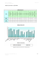
1
Gas Storage Field Deliverability Enhancement and Maintenance: An Intelligent Portfolio Management Approach. Final Report Reporting Start Date: September 1, 2004 Reporting End Date: December 31, 2006 Report prepared by: Shahab D. Mohaghegh, Ph.D. Principal Investigator Razi Gaskari, Ph.D. Co-Principal Investigator And Mr. Kazim Malik Petroleum & Natural Gas Engineering West Virginia University Morgantown, WV 26506 Telephone: 304.293.7682 Fax: 304.293.5708 Reporting Issue Date: January 2007 Subcontract No. 3040-WVRC-DOE-1779 Report prepared for: GSCT Consortium Director PSU/Energy Institute The Pennsylvania State University C211 Coal Utilization Laboratory University Park, PA 16802-2309 Telephone: 814.865.0531 Fax: 814.685.3248 Email: [email protected] Shahab D. Mohaghegh, Razi Gaskari & Kazim Malik January 2007 DISCLAIMER This report was prepared as an account of work sponsored by an agency of the United States Government. Neither the United States Government nor any agency thereof, nor any of their employees, makes any warranty, expressed or implied, or assumes no legal liability or responsibility for the accuracy, completeness, or usefulness of any information, apparatus, product, or process disclosed, or represents that its use would not infringe privately owned rights. Reference herein to any specific commercial product, process, or service by trade name, trademark, manufacturer, or otherwise does not necessarily constitute or imply its endorsement, recommendation, or favoring by the United States Government or any agency thereof. The views and opinions of authors expressed herein do not necessarily state or reflect those of the United States Government or any agency thereof. Subcontract No. 3040-WVRC-DOE-1779 Final Report 2 Shahab D. Mohaghegh, Razi Gaskari & Kazim Malik January 2007 ABSTRACT Portfolio management, a common practice in the financial market, is essentially an optimization problem that attempts to increase return on investment. The objective of this project is to apply the state-of-the-art in optimum portfolio management to the gas storage field in order to optimize the return on investment associated with well remedial operations. Each year gas storage operators spend hundreds of thousands of dollars on workovers, recompletions, and re-stimulations of storage wells in order to battle the decline in deliverability due to well damage with time. A typical storage field has tens if not hundreds of production wells. Each well will respond to remedial operations in its own unique way. The well’s response to the remedial operation is a function of a set of uncontrollable reservoir characteristics such as porosity and permeability and a set of controllable parameters such as completion and stimulation practices. The objective of this project is to identify the combination of best candidate wells for the remedial operations that will result in the most successful program each year, and consequently provides the highest return on investment. The project deliverable is a Windows-based software application that would perform the analysis and provide the list of wells and their corresponding remedial operation for each year based on the budget constraints identified by the user. The state-of-the-art in intelligent systems application that is currently being used extensively in the Wall Street is the methodology to achieve the objectives of this proposed project. This methodology includes a hybrid form of artificial neural networks, genetic algorithms and fuzzy logic. Columbia Gas Transmission Corporation is the industry partner of this project and cooperated with the research and development team in order to ensure successful completion of the project. The software application that is the deliverable of this project and is explained in much detail in this report is available to public free of charge. One important note about the software is that the current, publicly available version of the software includes a neural network model that has been developed for our industry partner based on the data that they made available. Once a storage operator decides to implement this software, they should contact the principal investigator of this project (Shahab D. Mohaghegh, Professor, Petroleum & Natural Gas Engineering, West Virginia University, Email: [email protected] - Tel; 304-293-7682 ext. 3405 – Web Site: http://shahab.pe.wvu.edu) and arrange for development of a neural network model for their specific storage field. In order to make the best use of capabilities of the software package, it is recommended that the storage filed have a minimum of 75 wells (wells with data that can be used for analysis). Subcontract No. 3040-WVRC-DOE-1779 Final Report 3 Shahab D. Mohaghegh, Razi Gaskari & Kazim Malik January 2007 TABLE OF CONTENTS Abstract …………………………………………………………………….. Table of Content …………………………………………………………….. List of Figures …………………………………………………………………….. List of Figures …………………………………………………………………….. Introduction …………………………………………………………………….. Executive Summary …………………………………………………………….. Experimental …………………………………………………………………….. Results & Discussions …………………………………………………….. Conclusions …………………………………………………………………….. References …………………………………………………………………….. Subcontract No. 3040-WVRC-DOE-1779 Final Report 3 4 5 7 8 9 10 11 102 103 4 Shahab D. Mohaghegh, Razi Gaskari & Kazim Malik January 2007 LIST OF FIGURES Figure 1. Well-bore data retrieved from a file …………………………… Figure 2. Correction of Wrong API number in data …………………………… Figure 3. Data addition and refinement for Well-bore Data …………………… Figure 4. Multiple Data Entries in Completion Table ……………………………. Figure 5. Well-bore data retrieved from a file ……………………………………… Figure 6. Data addition and refinement for Completion Data …………………… Figure 7. Perforation data retrieved from a file ……………………………………… Figure 8. Data addition and refinement for Perforation Data …………………… Figure 9. Perforation data retrieved from a file ……………………………………… Figure 10. Microfiche to Database process ………………………….………..… Figure 11. Different formats of Nitrogen Amount …………………………… Figure 12. Data addition and refinement for Stimulation Data ……………...…… Figure 13. Tubing head pressure profile for multi-point test …………………… Figure 14. Bottom-hole pressure profile for multi-point test …………………… Figure 15. Flow test 1 – Delta pressure squared vs. time …………………………….. Figure 16. Flow test 2 – Delta pressure squared vs. time ……………………………. Figure 17. Extended flow test – Delta pressure squared vs. time …………………… Figure 18. Log-log graph ……………………………………………………… Figure 19. Gas properties simulator …………………………………………… Figure 20. Calculation of true skin …………………………………………… Figure 21. Calculation of true skin from build up test ……………………………. Figure 22. Retrieving flow rate of an open flow test …………………………… Figure 23. Flow Diagram of Well Test Analysis procedure …………………… Figure 24. Neural Network Inputs and their source …………………………… Figure 25. Accuracy of training data for the Neural Net ……………………………. Figure 26. Accuracy of calibration data for the Neural Net …………………… Figure 27. Accuracy of verification data for the Neural Net …………………… Figure 28. Different option in the software that make it versatile …………………….. Figure 29. Data addition and refinement for well test data …………………… Figure 30. Screen shot of database showing different tables …………………… Figure 31. Main Screen of software …………………………………………… Figure 32. File Main options …………………………………………………… Figure 33. Screen shot of Template file …………………………………………… Figure 34. Comment that shows format of some cells in Template Excel file………… Figure 35. Import data from filled-out Template …………………………………… Figure 36. Remove all data from database…………………….…………………… Figure 37. Exit from file menu………………. …………………………………… Figure 38. Help menu options……….………. …………………………………… Figure 39. “about” screen from help menu……. …………………………………… Figure 40. Browsing through the well-bore data …………………………………… Figure 41. Well-bore tab …………………………………………………… Figure 42. Completion tab …………………………………………………… Figure 43. Perforation tab …………………………………………………… Figure 44. Stimulation tab …………………………………………………… Figure 45. Well-test tab …………………………………………………………….. Figure 46. Adding a complete new Well – well-bore tab …………………………… Figure 47. Adding a complete new Well - completion tab…………………………. Figure 48. Adding a complete new Well – entering data for wellbore …………… Subcontract No. 3040-WVRC-DOE-1779 Final Report 14 15 16 18 20 19 22 23 25 26 27 29 33 33 34 34 35 35 36 37 38 40 42 44 45 45 46 48 49 50 51 52 53 53 54 54 55 55 56 57 59 60 61 62 63 64 65 66 5 Shahab D. Mohaghegh, Razi Gaskari & Kazim Malik Figure 49. Adding a complete new Well – entering data for perforation …………… Figure 50. Adding a complete new Well – entering data for stimulation …………… Figure 51. Adding a complete new Well – entering data for well test …………… Figure 52. Result of adding a complete new well ……………………………………. Figure 53. Editing well data ………………………………………………………. Figure 54. Editing completion data …………………………………………… Figure 55. Saving completion data …………………………………………… Figure 56. Saved completion data …………………………………………… Figure 57. Deleting perforation record ……………………………………………. Figure 58. Finding a well …………………………………………………… Figure 59. Well-test Analysis Option in well-test tab ………………… Figure 60. Show Chart – Peak Day Rate ………………………………………….. Figure 61. Show Chart – Absolute Open Flow …………………………………. Figure 62. Show Chart – Skin …………………………………………………… Figure 63. Show Chart – All Well Tests …………………………………………… Figure 64. Well Test Analysis button …………………………………………… Figure 65. Well Test Analysis module …………………………………………… Figure 66. Well Test Analysis tool …………………………………………… Figure 67. Draw a line and calculate the slope …………………………………… Figure 68. Simplified well test analysis tool …………………………………… Figure 69. Simplified well test with one well test before or after stimulation………… Figure 70. LIT well test analysis ………………………………………….………… Figure 71. Multi point well test analysis ………………………………………….. Figure 72. Well extended pressure profile …………………………………… Figure 73. Selecting the build-up selection from pressure profile …………………… Figure 74. Diagnostic plot analysis …………….……………………………… Figure 75. Calculating skin from Hornet plot …………………………………… Figure 76. Selecting Ohio County ………….………………………………. Figure 77. Selecting wells according to stimulation year ………………………… Figure 78. Offset wells ……….………………………………………….. Figure 79. Selecting Well Parameters …………………………………………… Figure 80. Result of the wells & parameters selected ………………………...… Figure 81. Start Candidate Selection from main screen ………………………..… Figure 82. Candidate Selection main screen …………………….…………..… Figure 83. Selecting a well for candidate selection ……………………..…… Figure 84. Options to control Candidate Selection process …………………… Figure 85. Cost analysis Module ………………………………………..…………… Figure 86. Inputs that used to train the Neural Network ……………………….…… Figure 87. Select the controllable parameters in optimization process …………… Figure 88. Setup GA parameters ……………………………………………………. Figure 89. If one of the Neural Net input is well test before stimulation it could setup here. Figure 90. Optimization process for one well……………………………………… Figure 91. Optimization result for selected wells…………………………………… Figure 92. Rank the optimization result based on delta skin in order to find the best candidate Subcontract No. 3040-WVRC-DOE-1779 Final Report January 2007 66 67 67 68 71 72 73 74 75 76 77 77 78 78 79 80 80 82 83 83 84 85 86 87 89 90 91 91 92 92 93 94 95 95 99 97 99 99 100 100 100 101 101 101 6 Shahab D. Mohaghegh, Razi Gaskari & Kazim Malik January 2007 LIST OF TABLES Table 1. Draw down Test Results ……………………………………… Table 2. Build-up test results ………………………………..…………….... Table 3. Average Results ……………………………………………………………… Table 4. Calculation to determine the length of chromosome …………………………. Table 5. CA characteristic …………………………………………………………….. Subcontract No. 3040-WVRC-DOE-1779 Final Report 37 39 39 47 47 7 Shahab D. Mohaghegh, Razi Gaskari & Kazim Malik January 2007 INTRODUCTION Each year Gas Storage operators spend hundreds of thousands of dollars to combat the inevitable decline in the deliverability of their production wells. The decline in deliverability with time has two major contributors. The first contributor is geology and reservoir characteristics that are uncontrollable parameters. The second sets of parameters that contribute to the decline are associated with well damage that is addressed by well remedial operations such as workovers, recompletions, and re-stimulation of the producing wells. The parameters associated with these remedial operations can be controlled by the operator. It is a fact that every well will respond to a specific remedial operation in a unique way. For example, the deliverability of well “A” will increase two folds if a proper restimulation is performed on it while the same operation performed on well “B” will result in little or no deliverability enhancement. Same is true for workovers. Finding the best candidate for restimulation or workover, each year, among the tens or hundreds of wells is a challenging task. Consider another situation where well “C” will have a 70% increase if a restimulation is performed but it would have a 65% increase if a far less expensive workover is performed. Obviously performing a workover instead of a restimulation on well “C” would be more economical this year. Subcontract No. 3040-WVRC-DOE-1779 Final Report 8 Shahab D. Mohaghegh, Razi Gaskari & Kazim Malik January 2007 EXECUTIVE SUMMARY Portfolio management, a common practice in the financial market, is essentially an optimization problem that attempts to increase return on investment. The objective of this project is to apply the state-of-the-art in optimum portfolio management to the gas storage field in order to optimize the return on investment associated with well remedial operations. Each year gas storage operators spend hundreds of thousands of dollars on workovers, recompletions, and re-stimulations of storage wells in order to battle the decline in deliverability due to well damage with time. A typical storage field has tens if not hundreds of production wells. Each well will respond to remedial operations in its own unique way. The well’s response to the remedial operation is a function of a set of uncontrollable reservoir characteristics such as porosity and permeability and a set of controllable parameters such as completion and stimulation practices. The objective of this project is to identify the combination of best candidate wells for the remedial operations that will result in the most successful program each year, and consequently provides the highest return on investment. The project deliverable is a Windows-based software application that would perform the analysis and provide the list of wells and their corresponding remedial operation for each year based on the budget constraints identified by the user. The state-of-the-art in intelligent systems application that is currently being used extensively in the Wall Street is the methodology to achieve the objectives of this proposed project. This methodology includes a hybrid form of artificial neural networks, genetic algorithms and fuzzy logic. Columbia Gas Transmission Corporation is the industry partner of this project and cooperated with the research and development team in order to ensure successful completion of the project. The software application that is the deliverable of this project and is explained in much detail in this report is available to public free of charge. One important note about the software is that the current, publicly available version of the software includes a neural network model that has been developed for our industry partner based on the data that they made available. Once a storage operator decides to implement this software, they should contact the principal investigator of this project (Shahab D. Mohaghegh, Professor, Petroleum & Natural Gas Engineering, West Virginia University, Email: [email protected] - Tel; 304-293-7682 ext. 3405 – Web Site: http://shahab.pe.wvu.edu) and arrange for development of a neural network model for their specific storage field. In order to make the best use of capabilities of the software package, it is recommended that the storage filed have a minimum of 75 wells (wells with data that can be used for analysis). Subcontract No. 3040-WVRC-DOE-1779 Final Report 9 Shahab D. Mohaghegh, Razi Gaskari & Kazim Malik January 2007 EXPERIMENTAL No experimental work was performed during this project. Subcontract No. 3040-WVRC-DOE-1779 Final Report 10 Shahab D. Mohaghegh, Razi Gaskari & Kazim Malik January 2007 RESULTS & DISCUSSIONS This is the detail report of the progress made so far in the above mentioned project, which consists of following components: 12345- Project Overview Data made available and its format Neural Network Model Genetic Optimization Model Database & Software PROJECT OVERVIEW The objective of this project is to apply state-of-the-art intelligent, optimum portfolio management to the gas storage field in order to optimize the return on investment associated with well remedial operations. Columbia Gas Transmission Corporation is the industry partner in this project and provided us with very valuable data and in-depth knowledge about their gas storage field operations. The data in very crude form was provided to the research and development team in the last week of March, 2005. The team extracted valuable data and organized it in a form of database, with generic make up in order to be reusable. Windows-based software was developed which can help the user in viewing and later populating the data with easy to use interface. One of its modules provides the user with all the valid stimulations required as an input for Neural Network. A Neural Network was trained in order to predict skin for different stimulation parameters. A Genetic Optimization tool was developed and associated with the trained Neural Network in order to find the optimum stimulation parameters. The software ranks the well according to maximum change in skin value or/and stimulation cost for a well. Then a decision is made to restimulate a well or not accordingly. Subcontract No. 3040-WVRC-DOE-1779 Final Report 11 Shahab D. Mohaghegh, Razi Gaskari & Kazim Malik January 2007 DATA MADE AVAILABLE AND ITS FORMAT The research and development (R & D) team was initially provided data in MS excel worksheets. On further request, some pdf files with well schematics, well test files and well summary files were provided but still the required data especially relating to stimulations and well-tests was so scarce that the team in July, 2005 went to the Columbia Transmission Corporation Office in Charleston, WV to get more information. Retrieval of data from different files and thousands of microfiche was taking so long at the office that it was decided that West Virginia University lab facilities will be used to read thousands of microfiche. So, for the next few weeks the team concentrated its efforts on data collection. That data could be segregated into five main tables, each relating to specific characteristic features of the gas storage wells. The five characteristic features are as below: 123456- Well-bore data Completion Data Perforation Data Stimulation Data Well-Test Data Reservoir Characteristic Data Subcontract No. 3040-WVRC-DOE-1779 Final Report 12 Shahab D. Mohaghegh, Razi Gaskari & Kazim Malik January 2007 WELL BORE DATA It includes basic features of the well like location, depth, well name … etc. Data about well-bore was retrieved mostly from well schematics and well summary reports. The data already provided by Columbia Transmission Corporation was also verified. The complete list of the data type retrieved is as below: 1. 2. 3. 4. 5. 6. 7. 8. 9. 10. 11. 12. 13. 14. API Number Field Name Well Lease Name Classification Latitude (Lat) Longitude (Long) Section Township County State Operator Total Vertical Depth Formation Picture of one of the forms from which this data was retrieved is on next page Subcontract No. 3040-WVRC-DOE-1779 Final Report 13 Shahab D. Mohaghegh, Razi Gaskari & Kazim Malik January 2007 Fig1. Well-bore data retrieved from a file Subcontract No. 3040-WVRC-DOE-1779 Final Report 14 Shahab D. Mohaghegh, Razi Gaskari & Kazim Malik January 2007 The tables contained many minor mistakes like wrong Well API number, length, and many spelling mistakes. A picture of this correction is shown below: Fig2. Correction of Wrong API number in data Subcontract No. 3040-WVRC-DOE-1779 Final Report 15 Shahab D. Mohaghegh, Razi Gaskari & Kazim Malik January 2007 Analysis of raw data vs. refined data: Fig3. Data addition and refinement for Well-bore Data Subcontract No. 3040-WVRC-DOE-1779 Final Report 16 Shahab D. Mohaghegh, Razi Gaskari & Kazim Malik January 2007 COMPLETION DATA Completion data mostly relates to the type and depth of casing/liner/tubing run in the gas storage wells. The data type retained for the database includes the following: 1. 2. 3. 4. 5. 6. 7. 8. 9. 10. API Number Field Name Well Name (Well) Completion Description (Des) Date Tubing Run (Dt Tm Rn) Outer Diameter (OD) Top of Casing Bottom of Casing(Bot) Casing Weight (Weight) Casing Grade (Grade) Unfortunately the data was mostly in an excel file and had to be verified with well schematic drawings. This led to the most unusual step in this project as it lead to reduction of valuable data available to us. This was due to the erroneous and multiple data entry originally in the completion table. Identification of the multiple entries and their removal from table was the most focused act of cleaning the data, as omission of desirable records was unacceptable. Following pictures show one of such flawed multiple data entries which were removed. Subcontract No. 3040-WVRC-DOE-1779 Final Report 17 Shahab D. Mohaghegh, Razi Gaskari & Kazim Malik January 2007 Fig4. Multiple Data Entries in Completion Table In the completion table, the following notations used as casing description were replaced in place of different notations being used to have a standard definition Subcontract No. 3040-WVRC-DOE-1779 Final Report 18 Shahab D. Mohaghegh, Razi Gaskari & Kazim Malik January 2007 Completion data was mostly re- checked for accuracy from the documents, picture of which is shown below for a Well. Fig5. Well-bore data retrieved from a file Subcontract No. 3040-WVRC-DOE-1779 Final Report 19 Shahab D. Mohaghegh, Razi Gaskari & Kazim Malik January 2007 Analysis of raw data vs. refined data: Please note that multiple data entry was the major reason for the reduction in the refined data from the initial data. Fig6. Data addition and refinement for Completion Data Subcontract No. 3040-WVRC-DOE-1779 Final Report 20 Shahab D. Mohaghegh, Razi Gaskari & Kazim Malik January 2007 PERFORATION DATA This data set contains all the information relating to the perforations done on the gas storage well like perforation top & bottom depth and shots per foot. Following are the data types included in this type of data set: 1. 2. 3. 4. 5. 6. 7. 8. 9. Well API Number Field Name Well Name Completion Type Perforation Date (Perf Date) Perforation Top (Perf Top) Perforation Bottom (Perf Btm) Shot Type Shot Per foot (Shot Per ft) The picture of a document showing this information is shown below. Subcontract No. 3040-WVRC-DOE-1779 Final Report 21 Shahab D. Mohaghegh, Razi Gaskari & Kazim Malik January 2007 Fig7. Perforation data retrieved from a file Subcontract No. 3040-WVRC-DOE-1779 Final Report 22 Shahab D. Mohaghegh, Razi Gaskari & Kazim Malik January 2007 Analysis of raw data vs. refined data: Fig8. Data addition and refinement for Perforation Data Subcontract No. 3040-WVRC-DOE-1779 Final Report 23 Shahab D. Mohaghegh, Razi Gaskari & Kazim Malik January 2007 STIMULATION DATA Stimulation data is one of the most significant datasets about the storage wells. Because of this, it was very important that we have maximum records of valid stimulations. Following data type is used to represent stimulation: 1. 2. 3. 4. 5. 6. 7. 8. 9. 10. 11. 12. 13. 14. 15. 16. 17. 18. 19. 20. 21. 22. 23. API Well Number Well Name Size of String Stimulation From Stimulation To No Of Shots Fractured by Stimulation Type Stimulation Date Water Acid Gel Foam Nitrogen Alcohol Cushion Flush Sand Quantity Sand Type Injection Rate Total Fluid Breakdown Pressure ISIP Unfortunately, initially we didn’t have much data about the stimulations being done in this Lucas field. With this in mind, every record with Columbia Transmission Corporation was carefully examined. The largest source of stimulation data came from the thousands of microfiche with some data being found in well summary reports. Following is a picture of data in well summary reports. Subcontract No. 3040-WVRC-DOE-1779 Final Report 24 Shahab D. Mohaghegh, Razi Gaskari & Kazim Malik January 2007 Fig9. Stimulation data retrieved from a file Subcontract No. 3040-WVRC-DOE-1779 Final Report 25 Shahab D. Mohaghegh, Razi Gaskari & Kazim Malik January 2007 Fig10. Microfiche to Database process Subcontract No. 3040-WVRC-DOE-1779 Final Report 26 Shahab D. Mohaghegh, Razi Gaskari & Kazim Malik January 2007 Following are pictures of some types of data formats for fracture jobs found in the records Fig11. Different formats of Nitrogen Amount During the data entry different sign conventions and unit conversions were carried out as follows: Subcontract No. 3040-WVRC-DOE-1779 Final Report 27 Shahab D. Mohaghegh, Razi Gaskari & Kazim Malik January 2007 The following notations were used in place of different notations being used in the tables: All records of Nitro-shots were discarded for this database as they have no stimulation parameters on record and are part of history now plus they also damage the well. Above all, they will tend to degrade the Neural Network. Subcontract No. 3040-WVRC-DOE-1779 Final Report 28 Shahab D. Mohaghegh, Razi Gaskari & Kazim Malik January 2007 Analysis of raw data vs. refined data: Fig12. Data addition and refinement for Stimulation Data. Subcontract No. 3040-WVRC-DOE-1779 Final Report 29 Shahab D. Mohaghegh, Razi Gaskari & Kazim Malik January 2007 WELL TEST DATA Well-test data is the most extensive dataset that our R & D team worked on. It has the maximum amount of records nearly 3365 and 29 data types that control every aspect of a well-test. The data type selected for a well-test representation consists of following: 1. 2. 3. 4. 5. 6. 7. 8. 9. 10. 11. 12. 13. 14. 15. 16. 17. 18. 19. 20. 21. 22. 23. 24. 25. 26. 27. 28. 29. Well API Number Field Name Test Date Test Type Time 1 Field Pressure 1 Flowing Pressure 1 Rate 1 Time 2 Field Pressure 2 Flowing Pressure 2 Rate 2 Time 3 Field Pressure 3 Flowing Pressure 3 Rate 3 Time Extended Field Pressure Extended Flowing Pressure Extended Rate Extended kh Skin True Skin Non Darcy Co-efficient n Value C Value Delta Pressure Squared Peak Day Rate Absolute Open Flow Subcontract No. 3040-WVRC-DOE-1779 Final Report 30 Shahab D. Mohaghegh, Razi Gaskari & Kazim Malik January 2007 Estimation of n, C, peak day rate & absolute open flow Single/Open flow Tests: The values used for point 1 and 2 are from different well-tests 1- Find ∆P2 2 2 3- 2 2 1 log( p − pwf ) 2 − log( p − pwf )1 = n log q2 − log q1 4- C= 5- AOF = C (11502 − 02 ) n 6- PDRate = (C × 250, 000) n McfD qg 2 ( p − pwf 2 ) n (Where q is in MMcfD) (Where q is in McfD) McfD Multi-Point Tests: Estimation of n, C, PD rate & AOF: Same as above except that the points used are from the same test NOTE: The n, C, PD rate & AOF values for more than 400 well-tests were manually calculated Subcontract No. 3040-WVRC-DOE-1779 Final Report 31 Shahab D. Mohaghegh, Razi Gaskari & Kazim Malik January 2007 Estimation of kh, skin, true skin, non--darcy coefficient 1- From extended draw-down test plot (Pi-Pwf) vs. time on log-log paper. Draw unit-line for un-stimulated wells and half-slope line for Stimulated wells. Find end of well-bore storage effects after 1-1/2 log time cycle 2- Find values of viscosity, z-factor, compressibility of storage gas at different pressure assuming Gas gravity = 0.585 & temperature = 75 F = 535 R Draw-Down Test: 1234- 5678- Plot Pwf2 vs. time Draw straight line after pseudo-steady state starts Find slope m and P21hr 1637qTzu kh = m ⎡ p 2 − p 21hr ⎤ ⎛ k ⎞ − log ⎜ + 3.23⎥ S = 1.151 ⎢ 2 ⎟ m ⎢⎣ ⎥⎦ ⎝ φµ crw ⎠ Plot skin vs. flow-rate. It should be a straight line Slope of this line is D Find True Skin (S') at q=0. Build-Up Test: 1- Plot Pwf2 vs. (tp+dt)/dt on semi-log paper 2- Draw straight line after well-bore storage effects diminishes 3- Find slope m and P21hr 1637qTzu 4- kh = m ⎡ p2 − p2 ⎤ ⎛ k ⎞ − log ⎜ + 3.23 5- S = 1.151 ⎢ 1hr ⎥ ⎟ 2 m ⎝ φµ crw ⎠ ⎣⎢ ⎦⎥ 6- Plot skin vs. flow-rate. It should be a straight line 7- Slope of this line is D 8- Find True Skin (S') at q=0. We require time, flow-rate & Bottom hole pressure from the data which are present in two txt files as bottom hole & surface recording files. The flow rates are at Wellhead so we match the BHP & THP with time. Subcontract No. 3040-WVRC-DOE-1779 Final Report 32 Shahab D. Mohaghegh, Razi Gaskari & Kazim Malik January 2007 Fig13. Tubing Head Pressure profile for Multi-Point test Fig14. Bottom Hole Pressure profile for Multi-Point test The multipoint-test data is divided into Draw-down & build-up test and each one is analyzed separately. Subcontract No. 3040-WVRC-DOE-1779 Final Report 33 Shahab D. Mohaghegh, Razi Gaskari & Kazim Malik January 2007 Draw-down test Analysis of drawdown tests was done as described above and following graphs were obtained Fig15. Flow Test 1 – Delta pressure squared vs. time Fig16. Flow Test 2 – Delta pressure squared vs. time Subcontract No. 3040-WVRC-DOE-1779 Final Report 34 Shahab D. Mohaghegh, Razi Gaskari & Kazim Malik January 2007 Fig17. Extended Flow Test – Delta pressure squared vs. time Fig18. Log-log graph Subcontract No. 3040-WVRC-DOE-1779 Final Report 35 Shahab D. Mohaghegh, Razi Gaskari & Kazim Malik January 2007 For well-tests after fracture half-slope line is drawn and for un-simulated wells unit slope line is drawn to find end of well-bore effects and start of pseudo-steady state. Gas production Simulator was used to find the values of viscosity, z-factor and compressibility of storage gas at different pressure assuming Gas gravity = 0.585 & Temperature = 75 F = 535 R that are also used by Columbia Trans. Fig19. Gas Properties Simulator The slope from Pwf^2 vs. time on semi-log graph was used to find kh & then skin. The three values of skin were plotted on Q vs. S graph and extrapolated to Q = 0 to get True skin (S’). Subcontract No. 3040-WVRC-DOE-1779 Final Report 36 Shahab D. Mohaghegh, Razi Gaskari & Kazim Malik January 2007 Fig20. Calculation of True skin Table 1. Draw down Test Results Subcontract No. 3040-WVRC-DOE-1779 Final Report 37 Shahab D. Mohaghegh, Razi Gaskari & Kazim Malik January 2007 Build-up test In build-up tests, the slope drawn for Horner plot is after the time when well-bore storage effects were found to be minimizing from previous draw-down test. This slope is then used to find the values of kh & skin. The True skin is found the similar way as in draw-down test. Fig21. Calculation of True skin Build-up test Subcontract No. 3040-WVRC-DOE-1779 Final Report 38 Shahab D. Mohaghegh, Razi Gaskari & Kazim Malik January 2007 Table 2. Build-up test results Table 3. Average Results Due to large errors corresponding to estimating skin and kh values manually, it was decided that for time being these values will not be entered in the database. Subcontract No. 3040-WVRC-DOE-1779 Final Report 39 Shahab D. Mohaghegh, Razi Gaskari & Kazim Malik January 2007 Following are some pictures of the documents to show the different format in which the data was presented in files and microfiche. Fig22. Retrieving flow-rate of an open-flow test Subcontract No. 3040-WVRC-DOE-1779 Final Report 40 Shahab D. Mohaghegh, Razi Gaskari & Kazim Malik January 2007 Laminar Inertial Turbulent (LIT) Test Analysis of data from isochronal type test using Laminar Inertial Turbulent (LIT) flow equation will yield considerable data. This method can also be used to find skin of a well from singlepoint test when the value of permeability of reservoir is known from prior multi-point test. The LIT equation is written as: ∆ψ = ψ R − ψ wf = at q sc + bq sc2 Pressure drop due to Pressure drop due to laminar inertial-turbulent flow flow and well conditions Procedure for calculating Skin from LIT analysis for known permeability (k) value is as shown below: 1. Calculate at and b from equations below: ∆Ψ at ∑ q ∑ q − ∑ q ∑ ∆Ψ = N∑q − ∑q ∑q 2 sc sc sc 2 sc sc sc ∆Ψ N ∑ ∆Ψ − ∑ q sc ∑ q sc b= 2 N ∑ q sc − ∑ q sc ∑ q sc N= Number of data points 2. Plot ( ∆Ψ − bqsc2 ) vs. qsc on a logarithmic scale. The transient data points should form a 3. straight line. If they don’t form a straight line, calculate at and b again with the data which forms the straight line. Calculate Skin (S) with the formula. S= ⎤ ⎛ kt ⎞ 1 ⎡ kh 6 − log ⎜ + 3.23⎥ ⎢ at ×10 6 2 ⎟ 0.869 ⎣⎢ 1.632 × 10 T ⎝ φµi ci rw ⎠ ⎦⎥ Where: ∆Ψ : Delta Pseudo Pressure k : Effective permeability to gas, md h : Net pay thickness, ft t : Flow time, hrs : Porosity, % : Initial Viscosity, cp ui : Initial compressibility, psi-1 ci T : Temperature of the reservoir, oR : Well-bore radius, ft rw S : Skin, dimensionless Subcontract No. 3040-WVRC-DOE-1779 Final Report 41 Shahab D. Mohaghegh, Razi Gaskari & Kazim Malik January 2007 Flow Diagram of Well Test Analysis procedure Following is the flow diagram of the well test analysis procedure and the type of values that we get from the data. Fig23. Flow Diagram of Well Test Analysis procedure Subcontract No. 3040-WVRC-DOE-1779 Final Report 42 Shahab D. Mohaghegh, Razi Gaskari & Kazim Malik January 2007 RESERVIOR CHARACTERISTIC It includes some reservoir properties. The complete list of the data type retrieved is shown below: 1. 2. 3. 4. 5. 6. API Number Well Radius Reservoir Porosity Reservoir Temperature Gas Specific Gravity Reservoir Thickness Subcontract No. 3040-WVRC-DOE-1779 Final Report 43 Shahab D. Mohaghegh, Razi Gaskari & Kazim Malik January 2007 NEURAL NETWORK MODULE The Neural nets are very powerful in predicting non-linear relationships. As the relationship between skin and stimulation parameters is non-linear and very complicated, thus neural nets are used which are very good at it. With skin values before and after the stimulation calculated and stimulation parameters known, we can now use these valid stimulations to train the Neural Network to use it as a prediction tool. Intelligent Data Evaluation and Artificial Network IDEA® software by Intelligent Solutions Inc. was used to design the neural network. This software is very versatile in making different nets with different training algorithms. Generalized Regression Neural Net (GRNN) was used to train the neural net. The net had 11 inputs and 1 output as skin. The source of data for the neural net is given in Figure 24. Fig24. Neural Network Inputs and their source Out of the 78 valid stimulations available, the Neural net was trained on 60 data items while 14 were used as calibration data and 4 as verification data. The Neural network showed very good results for all three types of data. The screen shot taken from the IDEA software for training of the neural net is shown in Figure 25. Subcontract No. 3040-WVRC-DOE-1779 Final Report 44 Shahab D. Mohaghegh, Razi Gaskari & Kazim Malik January 2007 Fig25. Accuracy of training data for the Neural Net The calibration and verification of the Neural net is shown in Figure 26 and Figure 27 respectively. After the accurate results of this GRNN, the software was updated to use the GRNN generated files to be used in the Genetic algorithm. Fig26. Accuracy of calibration data for the Neural net Subcontract No. 3040-WVRC-DOE-1779 Final Report 45 Shahab D. Mohaghegh, Razi Gaskari & Kazim Malik January 2007 Fig27. Accuracy of verification data for the Neural net Subcontract No. 3040-WVRC-DOE-1779 Final Report 46 Shahab D. Mohaghegh, Razi Gaskari & Kazim Malik January 2007 GENETIC OPTIMIZATION MODEL Genetic Algorithm was written to optimize the stimulation parameters used in the neural net. Out of the 11 input parameters, 7 can be varied to obtain optimum skin. The range of these variables was calculated and accuracy desired was determined to design the length of the chromosome of Genetic Algorithm (GA) that will be required. The calculation is shown in the table 4. for the chromosome length if all the parameters are selected. Table 4. Calculation to determine the length of chromosome The length of chromosome came out to be 9 + 11 +10 + 8 + 9 + 9 + 2 = 58. The GA characteristics that were used are shown in Table 5. These were the best but can be changed as desired to suit other neural nets in the future. Table 5. CA characteristic There are two optimization methods made available in this software. One is optimization just based on skin and other, based on both skin and cost. The optimization objective function is calculated using the following formula and GA minimizes this optimization objective function. Subcontract No. 3040-WVRC-DOE-1779 Final Report 47 Shahab D. Mohaghegh, Razi Gaskari & Kazim Malik January 2007 Software compatibility and variability: In the software user has been given many options to accommodate the particular situation that he has and data availability if different from the data that we have used to verify the results from this software. Fig28. Different options in the software that makes it versatile. One of such variability introduced is that the software can use any other neural net if it is required. The option menu of the optimization screen has the option to import any other neural network. Plus, there is an option to select the available controllable parameters for the GA. For example, if the user does not want to use or does not have foam and nitrogen, then he can unselect them as shown in Figure 3.18. The length of GA will change according to the selection. As the Neural Net has ‘Well-Test Type’ as its input, so the ‘Select Well-Test Type’ menu option gives the user an option to choose the test the user wants the neural net to interpret the well-test. With changing price of hydro-carbons, the petroleum industry is going through fluctuating material cost. The stimulation material prices change frequently and are a factor of demand and supply in that region. The software has the option to change the price of the stimulation material before applying the GA to the available data. Subcontract No. 3040-WVRC-DOE-1779 Final Report 48 Shahab D. Mohaghegh, Razi Gaskari & Kazim Malik January 2007 Analysis of raw data vs. refined data: Fig29. Data addition and refinement for well test data Subcontract No. 3040-WVRC-DOE-1779 Final Report 49 Shahab D. Mohaghegh, Razi Gaskari & Kazim Malik January 2007 DATABASE & SOFTWARE SOFTWARE BASICS This software allows you to add/edit well data in the database and choose the data that you want to look at, for a selected well. It also has a Well Test Analysis tool which calculates the well deliverability parameters like n, C, Peak Day rate & Absolute Open Flow The database for this software consists of five main tables 1. 2. 3. 4. 5. 6. Well bore Data Completion Data Perforation Data Stimulation Data Well Test Data Reservoir Characteristic Data The API number of a well is the primary key in this database so it must be known before adding a record and cannot be duplicated Fig30. Screen shot of database showing different tables Subcontract No. 3040-WVRC-DOE-1779 Final Report 50 Shahab D. Mohaghegh, Razi Gaskari & Kazim Malik January 2007 The software starts with the main menu screen with six options Fig31. Main Screen of software Complete list of items and sub-items in the above command buttons is shown below: File o Create Template o Import Data from filled-out Template o Remove all data from database o Exit Help o User Manual o Formulas o About Edit Well Data o Well bore o Completion o Stimulation o Perforation o Stimulation o Well Test • Well Test Analysis Tool o Reservoir o Find a Well View Well Data Subcontract No. 3040-WVRC-DOE-1779 Final Report 51 Shahab D. Mohaghegh, Razi Gaskari & Kazim Malik January 2007 o Select State & county o Select Wells o Selection Options o Select Well Data Candidate Selection File The file menu can be accessed from the top left corner of menu bar. It contains four options. o Create Template o Import Data from filled-out Template o Remove all data from database o Exit Fig32. File Menu options Create Template By executing this option first the user need to select a location in hard drive in order to save Template file. Once the Template is successfully created in the hard drive, a message will appear indicating the user that the template file has been created. Following is the screen shot of the Template file showing the Well bore data. Subcontract No. 3040-WVRC-DOE-1779 Final Report 52 Shahab D. Mohaghegh, Razi Gaskari & Kazim Malik January 2007 Fig33. Screen shot of Template file It has six worksheets, each representing the table in the database of the software. o Well bore Data o Completion Data o Stimulation Data o Perforation Data o Stimulation Data o Well Test Data o Reservoir Characteristic 1. These are the fields of the table. Each field represents one characteristic of the table and each row is one record. If the user is not clear about any field, then he/she can drag the screen cursor to that field name and the comment will appear like in the picture below where it will give a little explanation, its format and an example so that the user understands what sort of data to enter in each field Fig34. Comments that shows format of some cells in Template Excel file Subcontract No. 3040-WVRC-DOE-1779 Final Report 53 Shahab D. Mohaghegh, Razi Gaskari & Kazim Malik January 2007 2. This section has two sets of warnings for the user entering data. One is to not edit or change number of Titles in all the worksheets or worksheet names and the other is to add only unique 'API Number' in worksheet 'Well bore Data' and all dates in worksheets where required. This has been done as the data is retrieved from the template according to some specific format and non presence of any data in elementary field might stop program from using that record. All the elementary fields’ background is orange/red while others are in green. 3. This section shows all the worksheets in the Template file. Import Data from filled-out Template Fig35. Import data from filled-out Template If this option is selected from the file menu, then the program will ask the user to select the filled Template file from the location. The new data will be appended to the existing data. Remove all data from database If the user doesn’t want to append the data to the previous database but instead wants to up-load a whole new data, then there is an option in file menu as highlighted in the snapshot below. This option will remove all data in the previous database. After removing the data from previous database, the user can up-load the updated data from the template or enter it in the software. Fig36. Remove all data from database Subcontract No. 3040-WVRC-DOE-1779 Final Report 54 Shahab D. Mohaghegh, Razi Gaskari & Kazim Malik January 2007 Exit The program can be exited by two options. One is to exit by using the file menu and selecting ‘Exit’ while the other is to select the cross on the top right corner as in normal windows based applications. Fig37. Exit form file menu Help Another option that can be accessed from the menu bar on top of the main menu screen is the Help menu option. Fig38. Help menu options Subcontract No. 3040-WVRC-DOE-1779 Final Report 55 Shahab D. Mohaghegh, Razi Gaskari & Kazim Malik January 2007 It contains three types of information one is the User Manual for this software and second is the Formulas used in this software and third ‘About’ form which shows the system information and software contributors. Fig39. “about” screen form help menu Subcontract No. 3040-WVRC-DOE-1779 Final Report 56 Shahab D. Mohaghegh, Razi Gaskari & Kazim Malik January 2007 Edit/View Well Data This screen has all the well data in the form of five tabs (for five database tables) that can be edited / viewed or a Well Test Analysis can be performed in the Well Test tab. Fig40. Browsing through the well-bore data To browse between different wells To move to the first well, previous well, next well & the last well in the record, click on the button assigned to it. The records are sorted in ascending order according to well number API Number & Well Count Subcontract No. 3040-WVRC-DOE-1779 Final Report 57 Shahab D. Mohaghegh, Razi Gaskari & Kazim Malik January 2007 The progress bar shows the relative position of the record and well count shows the current well position in the well bore database out of the total records. The API number of the current well is also displayed Back to main menu Takes you back to the very first screen of the program Editing Tools These buttons will help you to add a new record, edit or delete it or find a well for which you want the data to be retrieved if you know its API number. Subcontract No. 3040-WVRC-DOE-1779 Final Report 58 Shahab D. Mohaghegh, Razi Gaskari & Kazim Malik January 2007 Different Tabs WELL BORE: Fig41. Well-bore tab This tab contains all the data pertaining to the name, location & some main features of the current well. Subcontract No. 3040-WVRC-DOE-1779 Final Report 59 Shahab D. Mohaghegh, Razi Gaskari & Kazim Malik January 2007 COMPLETION: Fig42. Completion tab This tab contains all the data relating to different completion run in the well. To browse between different Completions To move to the first completion, previous completion, next completion & the last completion in the record, click on the button assigned to it. The completions are assorted in ascending order according to date tubing run for current well. Subcontract No. 3040-WVRC-DOE-1779 Final Report 60 Shahab D. Mohaghegh, Razi Gaskari & Kazim Malik January 2007 PERFORATION: Fig43. Perforation tab To browse between different Perforations To move to the first perforation, previous perforation, next perforation & the last perforation in the record, click on the button assigned to it. The perforations are sorted in ascending order according to perforation date for current well. Subcontract No. 3040-WVRC-DOE-1779 Final Report 61 Shahab D. Mohaghegh, Razi Gaskari & Kazim Malik January 2007 STIMULATION: Fig44. Stimulation tab To browse between different Stimulations To move to the first stimulation, previous stimulation, next stimulation & the last stimulation in the record, click on the button assigned to it. The stimulations are sorted in ascending order according to stimulation date for current well. Subcontract No. 3040-WVRC-DOE-1779 Final Report 62 Shahab D. Mohaghegh, Razi Gaskari & Kazim Malik January 2007 WELL TEST: Fig45. Well-test tab To browse between different Well Tests To move to the first well test, previous well test, next well test & the last well test in the record, click on the button assigned to it. The well tests are sorted in ascending order according to well test date for current well. Adding a new data One can add a complete new well or just only a new well-bore/completion/perforation/ stimulation/well-test data by following method Adding a complete new well data 1- Click on the Add New button Subcontract No. 3040-WVRC-DOE-1779 Final Report while keeping your well bore tab as active. 63 Shahab D. Mohaghegh, Razi Gaskari & Kazim Malik January 2007 Fig46. Adding a complete new Well – well-bore tab The following messages will pop-up. If you want to add the complete new well-bore data then click No button . If you don’t have the dates of Stimulation, Completion, Perforation & Well-Test data, then click Yes and then add them one-by one. Following screen appears if No is clicked: Subcontract No. 3040-WVRC-DOE-1779 Final Report 64 Shahab D. Mohaghegh, Razi Gaskari & Kazim Malik January 2007 Fig47. Adding a complete new Well - completion tab The background color of text boxes of all tabs including well-bore tab will be yellow indicating that they are ready for entering data. 2- Enter the data in all the tabs. The dates for completion, perforation, stimulation & well test job should be known. Subcontract No. 3040-WVRC-DOE-1779 Final Report 65 Shahab D. Mohaghegh, Razi Gaskari & Kazim Malik January 2007 Fig48. Adding a complete new Well – entering data for wellbore Fig49. Adding a complete new Well – entering data for perforation Subcontract No. 3040-WVRC-DOE-1779 Final Report 66 Shahab D. Mohaghegh, Razi Gaskari & Kazim Malik January 2007 Fig50. Adding a complete new Well – entering data for stimulation Fig51. Adding a complete new Well – entering data for well test Subcontract No. 3040-WVRC-DOE-1779 Final Report 67 Shahab D. Mohaghegh, Razi Gaskari & Kazim Malik January 2007 3- Click the Save button Result of adding of complete well data Fig52. Result of adding a complete new well Warnings – If API Number is not entered Warnings – If API Number entered is already in the database Subcontract No. 3040-WVRC-DOE-1779 Final Report 68 Shahab D. Mohaghegh, Razi Gaskari & Kazim Malik Note: January 2007 The dates for completion, perforation, stimulation & well test should always be entered as the output of the software is directly dependent on the chronology of events. The format of date is also specified for the user where required. A close picture of that format is below: You need to enter API well number only once in the well-bore tab and it will be automatically copied in the rest of tabs and procedure is the same for editing. The format for entering well API Number is: If wrong format or well API number is entered for a new well, then you will be greeted with the following message Adding only well-bore/completion/perforation/stimulation/well-test data 1- Click on the Add New button you want to add the data. while keeping that tab active for which Only for well-bore tab following message pops up: Subcontract No. 3040-WVRC-DOE-1779 Final Report 69 Shahab D. Mohaghegh, Razi Gaskari & Kazim Malik Click Yes January 2007 button to add only Well-bore data. The background color of all text boxes of that tab will be yellow indicating that they are ready for entering data. 2- Enter the data. The dates for completion, perforation, stimulation & well test job should be known. 3- Click the Save button . Editing data One can edit complete well or just only a new well-bore/completion/perforation/ stimulation/well-test data by following methods: Editing a complete well data 1- Click on the Edit button Subcontract No. 3040-WVRC-DOE-1779 Final Report while keeping your well bore tab as active. 70 Shahab D. Mohaghegh, Razi Gaskari & Kazim Malik January 2007 Following screen pops up: Select accordingly. Fig53. Editing well data Subcontract No. 3040-WVRC-DOE-1779 Final Report 71 Shahab D. Mohaghegh, Razi Gaskari & Kazim Malik January 2007 Fig54. Editing completion data The background color of text boxes of all tabs including well-bore tab will be yellow indicating that they are ready for entering data. 2- Enter the data in all the active tabs. The dates for completion, perforation, stimulation & well test job should be known. 3- Click the Save button Subcontract No. 3040-WVRC-DOE-1779 Final Report . 72 Shahab D. Mohaghegh, Razi Gaskari & Kazim Malik January 2007 Editing only completion/perforation/stimulation/well-test data 1- Click on the Edit button edit the data except well bore tab. while keeping that tab active for which you want to Fig55. Saving completion data The background color of all text boxes of that tab will be yellow indicating that they are ready for entering data. Enter the data. The dates for completion, perforation, stimulation & well test job should be known. Click the Save button . Subcontract No. 3040-WVRC-DOE-1779 Final Report 73 Shahab D. Mohaghegh, Razi Gaskari & Kazim Malik January 2007 Result of editing only completion data Fig56. Saved completion data Deleting data One can delete complete well or just only delete completion/perforation/ stimulation/well-test data by following methods: Deleting a complete well data 1- Click on Delete button while keeping your well bore tab as active Editing only completion/perforation/ stimulation/well-test data 1- Click on Delete button the data except well bore tab. Subcontract No. 3040-WVRC-DOE-1779 Final Report while keeping that tab active of which you want to delete 74 Shahab D. Mohaghegh, Razi Gaskari & Kazim Malik January 2007 Fig57. Deleting perforation record You will be greeted with the above message to make sure that delete button is not accidentally pressed. 2- Click on yes if you want the selected record to be deleted. Subcontract No. 3040-WVRC-DOE-1779 Final Report 75 Shahab D. Mohaghegh, Razi Gaskari & Kazim Malik January 2007 Undo the edit/add operation: To undo the edit or add operation before they can be saved click undo button Finding a well Follow the following procedure to find a well for which you have some idea of its API well number: Click on Find button The following screen is displayed: Fig58. Finding a well Subcontract No. 3040-WVRC-DOE-1779 Final Report 76 Shahab D. Mohaghegh, Razi Gaskari & Kazim Malik January 2007 WELL TEST ANALYSIS To perform well test analysis on a well and draw graph of Peak day rate and Absolute open flow, use the option / command buttons below: Fig59. Well-test Analysis Option in well-test tab Peak day, AOF, Skin, and all well test graph Select PD rate , AOF, Skin or All well Tests option button and then click on the Show button . The following screens will appear according to the option selected: Fig60. Show Chart – Peak Day Rate Subcontract No. 3040-WVRC-DOE-1779 Final Report 77 Shahab D. Mohaghegh, Razi Gaskari & Kazim Malik January 2007 Fig61. Show Chart – Absolute Open Flow Fig62. Show Chart – Skin Subcontract No. 3040-WVRC-DOE-1779 Final Report 78 Shahab D. Mohaghegh, Razi Gaskari & Kazim Malik January 2007 Fig63. Show Chart – All Well Tests WELL TEST ANALYSIS TOOL The user can do three types of Well Test Analysis in this software: 1- Simplified Analysis (for calculating n, C, PD rate & AOF) 2- LIT Analysis (for calculating Skin if ‘k’ is known) 3- Build-up Test Analysis (If Detailed Multi-Point Test data is available) Subcontract No. 3040-WVRC-DOE-1779 Final Report 79 Shahab D. Mohaghegh, Razi Gaskari & Kazim Malik January 2007 Fig64. Well Test Analysis button The analysis tools are very similar for Simplified and LIT Analysis except where mentioned. The interface below will appear when you select ‘Well Test Analysis’ button. It will give you a glimpse of what has happened on the well since it was drilled. Fig65. Well Test Analysis Module 1. This section contains all the data in a grid form API Number, Date of well test, Test Type, kh value, Skin value, Peak Day rate, Absolute Open Flow and information in ‘YES’ or ‘NO’ form if the Detailed Multi-point data (Pressure profile & flow-rate vs. Subcontract No. 3040-WVRC-DOE-1779 Final Report 80 Shahab D. Mohaghegh, Razi Gaskari & Kazim Malik January 2007 time) is available for a given test or not. The back color of selected well-test is yellow while of stimulation is purple. The first well-test is selected by default. 2. This section contains instructions as how to select well-tests for analysis. Single click on any well-test will make it the current well-test with background changed to yellow and by double click; it will be selected for Simplified and LIT Analysis. If the Detailed MP Data for a well-test is given, then it can be selected for permeability analysis (build-up test) by single click on the cell where ‘YES’ is written. This way the build-up test analysis module will show up. 3. This section shows the time of different well tests which are indicated by three types of markers and stimulations on a well which are represented by straight blue vertical lines. The selected well have the similar marker according to its test-type but its color is dark green. Once any well-test is double clicked, it is selected and added in the list box of simplified and LIT Analysis. Subcontract No. 3040-WVRC-DOE-1779 Final Report 81 Shahab D. Mohaghegh, Razi Gaskari & Kazim Malik January 2007 Simplified Analysis: The screen shot of Simplified Analysis tab is below with Well-test # 2 to # 7 selected for analysis. Fig66. Well Test analysis tool 1. This section contains the list box which has the entire well-tests selected for an analysis. Any test now again can be selected or de-selected by using the check-box in front of it. Once the well-tests are selected, then they can be drawn on log-log graph of Flow-rate (McfD) vs. Delta Pressure Square (Delta P sqr) by selecting the ‘Draw Points’ button. This graph can be cleared by selecting the ‘Clear>>’ button also if the well-tests drawn need to be changed. 2. Once the data points have been drawn, the user can draw a line in the picture box keeping left mouse button held down like shown below: Subcontract No. 3040-WVRC-DOE-1779 Final Report 82 Shahab D. Mohaghegh, Razi Gaskari & Kazim Malik January 2007 Fig67. Draw a line and calculate the slope Select ‘Calculate n’ button to find the slope of the drawn line. The slope will be calculated in front of ‘n’ text box. 1. Now the user can select the well-tests that he/she intended to the simplified analysis on them. Then a line should draw based on the selected well tests in the picture box (Figure 68). The slop (n) will be calculated by mouse clicking on the “Calculate n” Button. The values of C, Peak Day Rate and Absolute Open Flow will be calculated and shown in the grid as shown in the picture shot on next page. These results can be saved in the database by selecting the ’Save’ button. Fig68. Simplified well test analysis tool Subcontract No. 3040-WVRC-DOE-1779 Final Report 83 Shahab D. Mohaghegh, Razi Gaskari & Kazim Malik January 2007 Note: If there is only one well-test before or after the stimulation, then the value of n can be assumed and written in the textbox in front of label ‘n’ as shown in the picture below. The value of ‘n’ cannot be assumed for more than one well at a time so if there is more than one well-test for which the value of ‘n’ has to be assumed, then they should be selected one by one. Fig69. Simplified well test with one well test before or after stimulation Subcontract No. 3040-WVRC-DOE-1779 Final Report 84 Shahab D. Mohaghegh, Razi Gaskari & Kazim Malik January 2007 Laminar Inertial Turbulent (LIT) test Analysis: The screen shot of the LIT analysis is below: Fig70. LIT well test analysis 1. This section is the same as for Simplified Analysis. 2. In this section, the well-test points are drawn on log – log plot of ‘Flow rate (MMcfD) vs. Delta pseudo pressure – bq2’ . There is no need to draw a slope line in this plot. Instead, the points can be selected by visual inspection that they form a straight line and that they were conducted preferably within 2 years. In the snapshot above, well test points 2,3 and 5 have been selected to calculate Skin. 3. When the ‘Calculate’ button is pressed, the program uses the permeability value ‘k’ from the nearest well-test and calculates skin. The new value of skin can be saved in the database by selecting ‘Save Results’ button. Note: Multi-point test points give erroneous calculations if selected with other well-tests as they are recorded one flow after another simultaneously, not like Open Flow and single point tests, which are recorded once a year. If the selected well-tests are not within 2 years, then the following message will appear giving the user choice either to select other well-tests or continue with the well-tests selected. Subcontract No. 3040-WVRC-DOE-1779 Final Report 85 Shahab D. Mohaghegh, Razi Gaskari & Kazim Malik January 2007 Build-up test Analysis: If any Multi-point well test has a detailed data (pressure and flow-rate profile vs. time), then the ‘Detailed MP Data’ column in front of that test will show ‘YES’. It means that the data for this well-test can be analyzed to estimate a value of permeability. Fig71. Multi point well test analysis Subcontract No. 3040-WVRC-DOE-1779 Final Report 86 Shahab D. Mohaghegh, Razi Gaskari & Kazim Malik January 2007 If the cell with value ‘YES’ is selected the software will read the data from the excel file and progress bar will become visible like in the picture shot above showing that the data is being read. After the complete data has been read by the software, the following screen will appear showing the pressure profile of the well-test. Fig72. Well extended pressure profile All the Input data is retrieved from the database and if it is not found, then default values are inserted. The value ’tp (flow/production time’ is 2 hrs by default but can be changed by the user. The Extended build-up test for 2 or more hours should be selected by keeping the left mouse button down. The green lines will indicate portion of build-up test selected. Subcontract No. 3040-WVRC-DOE-1779 Final Report 87 Shahab D. Mohaghegh, Razi Gaskari & Kazim Malik January 2007 Fig73. Selecting the build-up section from pressure profile If by mistake draw-down data is selected, then the following message will appear informing the user to select build-up data again. Subcontract No. 3040-WVRC-DOE-1779 Final Report 88 Shahab D. Mohaghegh, Razi Gaskari & Kazim Malik January 2007 After the portion of build-up data has been correctly selected, the permeability analysis tab will show following graphs. The first one is the log-log diagnostic plot between ‘Del Pressure’ and ‘Del Time’. The user should select the first point which does not fall on the unit slope line drawn by holding the left mouse button down. The initial pressure ‘Pi’ and flow rate text box values will be selected from the build-up portion of the extended well-test selected. The graphs will be drawn again with a green line drawn on the Horner plot indicating The End of Well-Bore Storage (tewbs). Fig74. Diagnostic plot analysis The slope should be drawn on the Horner plot on the left side of the end of well bore storage line shown in green on Horner plot. Subcontract No. 3040-WVRC-DOE-1779 Final Report 89 Shahab D. Mohaghegh, Razi Gaskari & Kazim Malik January 2007 Fig75. Calculating skin from Hornet plot After the slope is drawn, the user can select ‘Calculate Skin’ button to find the skin of the well. The respective graphs can be redrawn any time by selecting the ‘Redraw Diagnostic Plot’ or ‘Redraw Horner Plot’. The value of permeability and Skin can be saved in the database by selecting ‘Save’ button. Subcontract No. 3040-WVRC-DOE-1779 Final Report 90 Shahab D. Mohaghegh, Razi Gaskari & Kazim Malik January 2007 SELECT WELL DATA In this form the user can choose to select the data of the wells that he wants to look at. Following are a few ways he can choose the data: Selecting a well by State/County: The user selects the state first and then the county. All the wells will be selected for that county in the selected wells list box: Fig76. Selecting Ohio County Selecting wells by stimulation year: The user can select the option button for stimulated year and input the year values. If Select is clicked, then all the wells that have been stimulated between Wells button these years will be shown in the selected wells list box Subcontract No. 3040-WVRC-DOE-1779 Final Report 91 Shahab D. Mohaghegh, Razi Gaskari & Kazim Malik January 2007 Fig77. Selecting wells according to stimulation year Selecting offsets wells form a well: The user selects the offset option and the well near which he wants to find the off-set wells, and then enters the distance of off-set in kilometers. If Select Wells button is clicked, then all the wells that are off-set of the selected well will be shown in the selected wells list box Fig78. Offset wells Subcontract No. 3040-WVRC-DOE-1779 Final Report 92 Shahab D. Mohaghegh, Razi Gaskari & Kazim Malik January 2007 Display the selected wells data: When the wells for which the user want the data to be retrieved have been selected, click the and select the parameters. Select Well Data button Fig79. Selecting Well Parameters Click Show Well Data Subcontract No. 3040-WVRC-DOE-1779 Final Report to retrieve the data. 93 Shahab D. Mohaghegh, Razi Gaskari & Kazim Malik January 2007 Fig80. Result of the wells & parameters selected Subcontract No. 3040-WVRC-DOE-1779 Final Report 94 Shahab D. Mohaghegh, Razi Gaskari & Kazim Malik January 2007 CANDIDATE SELECTION This module will appear on selecting the ‘Candidate Selection’ button from Main Menu. Fig81. Start Candidate Selection form main screen For intelligent candidate selection of wells, it is very important that only valid data is given to the Neural Network (NN) for training. Valid data is one which will not degrade the performance of the NN and is useful in NN training. Fig82. Candidate Selection main screen Subcontract No. 3040-WVRC-DOE-1779 Final Report 95 Shahab D. Mohaghegh, Razi Gaskari & Kazim Malik 1. January 2007 When this module is loaded, each row in this section of the grid represents a valid stimulation as shown in figure above. Following, is the criteria for valid stimulation selection: Valid Stimulation – It should have skin value before & after stimulation. Valid Perforation – Perforation just before the stimulation. Valid Completion – The smallest size completion run before stimulation. Valid Well-test – Well-test having skin value just before or after the well-test. 2. Two types of analysis can be done on the wells: One option is to apply Genetic optimization on wells one at a time and the other is to apply it on all wells. If the ‘All Wells’ option is selected, then the ‘Select Well’ button will be enabled and the user can select the well the same way as shown in the previous section of the user Manual for – Find a well. Fig83. Selecting a well for candidate selection process 3. This section of module relates to the Optimization methods available. User can optimize the stimulations according to only change in skin criteria or may choose to select the ‘GA based on cost and skin’ option where he/she can give different weight ages to cost and skin. Subcontract No. 3040-WVRC-DOE-1779 Final Report 96 Shahab D. Mohaghegh, Razi Gaskari & Kazim Malik January 2007 Options Menu: This software can cater for many varied situations. These options can be selected from the ‘options’ menu bar on the top of the form. It contains following items: • • • • • • • Select controllable parameters Material cost Import NNet NNet Input values GA characteristic Export the Grid to Excel Select Well-Test Type Following is a screen shot of the items in the Options menu tool bar. Fig84. Options to control Candidate Selection process Material cost can be changed by the user as the prices fluctuate. These prices can be saved in the database by selecting ’Save’ button and Default values can be retrieved by selecting ‘ Default’ button. The screen shot of material cost is shown below and price is just an estimate and can be changed by user. Subcontract No. 3040-WVRC-DOE-1779 Final Report 97 Shahab D. Mohaghegh, Razi Gaskari & Kazim Malik January 2007 Fig85. Cost analysis module Fig86.Inpurs that used to train the Neural Network If the user wants to look at the Neural Network inputs being used, then ‘NNet Input’ option will take the user to a new form as shown above where all the inputs are shown. Keep in mind that this grid can only be seen once and that only after the Genetic optimization has been applied. If some material is not available for stimulation, then still the user can optimize the stimulation by de-selecting that material from the ‘Select controllable parameters’ option. The materials not enabled are the ones that are not being used by the Neural Network in use. Subcontract No. 3040-WVRC-DOE-1779 Final Report 98 Shahab D. Mohaghegh, Razi Gaskari & Kazim Malik January 2007 Fig87. Select the controllable parameters in optimization process A new Neural Network can be used if the data is changed or appended by importing its ‘ida’ file. When a new Neural Network is imported, it might change the optimum GA parameters. The user can change them from ‘GA characteristic’ option. The default values are always loaded at startup as shown in figure below but can be changed by user. Fig88. Setup GA pentameters If one of the Neural Net inputs is well test before stimulation, the type of the wells test in optimization process should specify here. Fig89. Type of the wells test in optimization process. Subcontract No. 3040-WVRC-DOE-1779 Final Report 99 Shahab D. Mohaghegh, Razi Gaskari & Kazim Malik January 2007 When all the parameters for GA have been selected and user selects the ‘Apply GA’ button, then the screen below will appear showing the values of optimized stimulation slurry and change in skin due to this stimulation. The picture below shows the GA optimization done on well # 12-345-67890. Fig90. Optimization process for one well Subcontract No. 3040-WVRC-DOE-1779 Final Report 100 Shahab D. Mohaghegh, Razi Gaskari & Kazim Malik January 2007 If the optimization is applied to all the wells, then we can rank the wells according to the change in skin by selecting ‘Rank the wells’ from Options menu bar on the top left corner of the form as shown in snapshot below. Fig91. Optimization result for selected wells The wells are ranked according to change in skin as shown in the figure below. These ranked wells and the optimized stimulation data now can be exported to excel by selecting ‘Export to Excel’ in the Option menu of Candidate Selection module. Fig92.Rank the optimization result based on delta skin in order to find the best candidates Subcontract No. 3040-WVRC-DOE-1779 Final Report 101 Shahab D. Mohaghegh, Razi Gaskari & Kazim Malik January 2007 CONCLUSION The main aim of this study was to find the re-stimulation candidate wells with the given data without trying to spend thousands of dollars on well-test and gas reservoir simulators. Detailed analysis of well-tests performed on the storage field was done and intelligent tools like Neural networks to predict the Skin and Genetic Algorithms were used to optimize the stimulation and to select the best stimulations for a well. The following conclusions can be drawn from this research: 1. The Artificial Intelligence Tool can predict Skin with high degree of confidence. 2. The Portfolio Management for re-stimulation candidate selection provides a cost effective method for taking full advantage of annual budget for remedial operations. 3. This software is the first successful attempt to combine Data editing, Well-Test analysis and Artificial Intelligence in one software package. Subcontract No. 3040-WVRC-DOE-1779 Final Report 102 Shahab D. Mohaghegh, Razi Gaskari & Kazim Malik January 2007 REFERENCES NONE Subcontract No. 3040-WVRC-DOE-1779 Final Report 103