1
Aero Troll
User’s Manual Supplement
v0.3.0b
by
Martin C. Hegedus
December 6, 2013
Copyright ©2013 by Martin C. Hegedus
Table of Contents
INTRODUCTION .............................................................................................................. 1
Intent ............................................................................................................................... 1
What’s New .................................................................................................................... 1
LICENSE ............................................................................................................................ 2
INSTALLATION ............................................................................................................... 3
BASIC EXAMPLE (NACA 0012)..................................................................................... 3
Startup ............................................................................................................................. 4
Main Menu Bar ............................................................................................................... 5
Problem Specification..................................................................................................... 5
First Off Surface Grid Spacing Determination ........................................................... 6
Geometry Setup .......................................................................................................... 8
Initial CFD Setup ...................................................................................................... 15
CFD Gridding ........................................................................................................... 20
View Translation and Zooming ................................................................................ 32
CFD Run Setup ......................................................................................................... 34
CFD Execution.......................................................................................................... 40
BASIC CONCEPTS ......................................................................................................... 54
Views ............................................................................................................................ 54
Segments ....................................................................................................................... 56
Line ........................................................................................................................... 56
Circular Arc .............................................................................................................. 57
Elliptical Arc............................................................................................................. 58
B-Spline .................................................................................................................... 59
Cubic Spline.............................................................................................................. 61
Stretching and Point Distribution.................................................................................. 62
Breaks ........................................................................................................................... 64
Adding Breaks .......................................................................................................... 64
Editing Breaks........................................................................................................... 65
Gridding ........................................................................................................................ 66
Sub Steps................................................................................................................... 72
Xi Volume and Slope................................................................................................ 75
Spread Start and Spread End..................................................................................... 82
Average Volume Weighting ..................................................................................... 85
CFD Execution Settings................................................................................................ 87
B.C. Settings ............................................................................................................. 87
Time Stepping Values............................................................................................... 88
CFD Display Settings ................................................................................................... 89
Plotting Contours .......................................................................................................... 90
WEDGE ............................................................................................................................ 91
Problem Specification................................................................................................... 93
Geometry Setup ........................................................................................................ 93
Initial CFD Setup .................................................................................................... 101
CFD Gridding ......................................................................................................... 107
CFD Run Setup ....................................................................................................... 126
ii
CFD Execution........................................................................................................ 137
MULTI-ELEMENT AIRFOIL ....................................................................................... 147
Problem Specification................................................................................................. 147
Slat Geometry ......................................................................................................... 149
Main Geometry ....................................................................................................... 161
Flap Geometry ........................................................................................................ 176
Initial CFD Setup .................................................................................................... 182
CFD Gridding ......................................................................................................... 184
CFD Run Setup ....................................................................................................... 216
CFD Execution........................................................................................................ 219
COMPONENTS ............................................................................................................. 227
Nose ............................................................................................................................ 228
Notes ........................................................................................................................... 231
Airfoil.......................................................................................................................... 232
NACA Airfoil Description...................................................................................... 232
User Defined 2D Shape .......................................................................................... 234
Menu Items ............................................................................................................. 234
Component Fields ................................................................................................... 235
NACA Input Section........................................................................................... 236
2D Geometry Input Section ................................................................................ 237
AT_Airfoil_CFD......................................................................................................... 239
Menu Items ............................................................................................................. 239
Commands .......................................................................................................... 240
Input .................................................................................................................... 240
Global Fields........................................................................................................... 241
Grid Fields .............................................................................................................. 241
CFD Fields .............................................................................................................. 242
Display Fields ......................................................................................................... 244
CFD Grid Group (Airfoil)........................................................................................... 246
Menu Items ............................................................................................................. 247
Commands .......................................................................................................... 247
Vol. Grid ............................................................................................................. 248
View.................................................................................................................... 248
Settings................................................................................................................ 249
Grid Type Field....................................................................................................... 250
Surface Grid Fields ................................................................................................. 250
Volume Grid Fields................................................................................................. 251
CFD Input Fields..................................................................................................... 253
CFD 2D Grid Block .................................................................................................... 254
Menu Items ............................................................................................................. 254
Commands .......................................................................................................... 255
View.................................................................................................................... 256
Settings................................................................................................................ 257
Surface Grid Fields ................................................................................................. 257
Volume Grid Fields................................................................................................. 258
CFD Input Fields..................................................................................................... 258
iii
Exec AT CFD Dialog.................................................................................................. 259
Exec AT CFD Dialog Fields................................................................................... 259
Exec AT CFD AT Cntrl Fields ............................................................................... 260
Exec AT CFD Run Cntrl Fields.............................................................................. 261
Exec AT CFD Flow Field Fields ............................................................................ 263
Exec AT CFD Resid Fields..................................................................................... 265
Exec AT CFD Turb Fields...................................................................................... 267
Exec AT CFD For+Mom Fields ............................................................................. 269
Exec AT CFD History Fields.................................................................................. 271
TOOLS/CALCULATORS ............................................................................................. 272
Standard Atmosphere.................................................................................................. 273
Y+ ............................................................................................................................... 275
Isentropic..................................................................................................................... 276
Shock........................................................................................................................... 278
Expansion.................................................................................................................... 280
iv
INTRODUCTION
Intent
Aero Troll is a preliminary aerodynamic analysis tool with a graphical user interface.
The goal of Aero Troll is to allow a user to describe and carry out aerodynamic analysis
on simplified geometries. The tool supports education, academic aerodynamic analysis,
and verification and validation efforts. The software was created to broaden my
knowledge of software development and aerodynamic modeling. It is hoped that the tool
will be helpful to others. Currently the code interfaces with a 2D Reynolds Averaged
Navier Stokes solver, PANAIR (A502), and a hypersonic impact method.
Aero Troll is available for Linux (32 and 64-bit) and Windows XP. Aero Troll has had
limited testing on Windows OSes other than XP.
All the required libraries have been included in the Aero Troll distribution. Aero Troll
requires Java 1.5 or later to be installed.
What’s New
The biggest addition to Aero Troll is a 2D Reynolds Averaged Navier Stokes (RANS)
solver. This manual describes how to run the 2D RANS method along with some, but not
all, changes. To run PANAIR and the impact method, the user is directed to the version
0.2.0b manual. It should be noted that the previous manual is outdated to some extent but
hopefully the user can figure things out. Hopefully a future manual will be more
complete.
New features:
1)
2)
3)
4)
5)
6)
7)
8)
2D RANS solver
Printing
Scripting tool
Additional view capabilities
Screen snapshots
Contour plotting
Tools/Calculators
a)
Standard Atmosphere
b)
y+
c)
Isentropic
d)
Shock
e)
Expansion
Components
a)
Airfoil
b)
Nose
c)
Notes
The scripting tool is not described in this manual and is left for a latter date.
1
LICENSE
Aero Troll License
Copyright (c) 2008-2013 Martin C. Hegedus.
All Rights Reserved.
Copying, reproduction, distribution, or publication of Aero Troll software is prohibited,
unless expressly authorized by Martin C. Hegedus. Aero Troll must be obtained from
www.hegedusaero.com or an authorized distributor.
This program and components are distributed in the hope that they will be useful, but
WITHOUT ANY WARRANTY; without even the implied warranty of
MERCHANTABILITY or FITNESS FOR A PARTICULAR PURPOSE. The software
is offered "AS IS". Martin C. Hegedus and those associated with the development and
distributions of any part of Aero Troll will not be liable to any party for any direct,
indirect, special, incidental, or consequential damages arising out of any use of this
software.
While every attempt has been made to identify and remove programming errors within
the software, there remains a high probability that programming errors remain. It is
possible that some of these errors could cause the results of an analysis to be incorrect. In
addition, the analysis results may also be affected by other identified, unidentified, and
unknown uncertainties and errors. The causes of these uncertainties and errors are, but
are not limited to, physical approximation, physical modeling, geometry modeling,
round-off, iterative convergence, discretization, and incorrect input.
Aero Troll and associated components are distributed WITHOUT ANY WARRANTY
that usage, errors, assumptions, uncertainties, or any other aspect associated with Aero
Troll, its components, and its analysis methods are documented or that documentation is
accessible to the end user.
It is the responsibility of the end user to accept all analysis answers with GREAT
CAUTION and SKEPTISM.
Aero Troll uses the following libraries, applications, and code:
PDAS PANAIR A502-ht2
PDAS NACA456
PDAS "Properties of the Standard Atmosphere"
JOGL 2.0-rc11
JavaPlot 0.4.0
gnuplot 4.6.3
CGNS 3.1.4
Jython 2.5.3
2
The licenses for these libraries and applications can be found by selecting the About
menu item under Aero Troll’s Help menu. The complete license is also in the Aero Troll
directory.
INSTALLATION
Two compressed archives exist. One of the archives, AeroTroll_v030b.tgz, is tarred and
gzipped. The other archive, AeroTroll_v030b.zip, is zipped. Please uncompress the one
appropriate for you.
Inside the uncompressed directory are four run scripts;
AeroTroll_win.bat, AeroTroll_win64.bat, AeroTroll_lin, and AeroTroll_lin64. Using the
run script appropriate for your system will start the Aero Troll application. The
application does not need to be installed by means of a script or install wizard.
Unpacking it is enough. The scripts do expect java to be in the execution path. The
scripts can be customized with a text editor. Currently a Mac version of Aero Troll for
CFD does not exist.
BASIC EXAMPLE (NACA 0012)
A NACA 0012 analysis will demonstrate the basic CFD usage of Aero Troll. For this
case the freestream conditions will be Mach 0.5, angle of attack 2.0 degrees, and a
Reynolds number of 3.0e6 based on the chord length. A Navier Stokes run will be
chosen with the Spalart Allmaras turbulence model. This example will get a user started;
however it will not demonstrate the full capabilities. Some of the capabilities and
components will be described in later sections and examples. Other capabilities will need
to be discovered by the user or by talking with others. It is also not the intent to teach the
user the ins and outs of CFD. For that, the user is referred to literature and the internet.
Before the user can search for relevant information about the method, the user must know
something about the CFD method used by Aero Troll. The CFD method used by Aero
Troll is a compressible implicit central difference method for the Reynolds Averaged
Navier-Stokes (RANS) equations in conservation law form for a calorically perfect gas
and for structured overlapping (Chimera) grids. A scalar artificial dissipation method is
used. The method employed by Aero Troll is first order accurate in time and second
order accurate spatially. Both constant and local time stepping methods are available.
Wall functions and Mach number preconditioning are not available at this time. Since
Mach number precondition is not implemented, very low Mach number runs will not
converge well and the results may be inaccurate due to numerical dissipation.
3
It should be noted, for the current version of Aero Troll, only the geometry and input
parameters are saved. The solution is not saved. Therefore, CFD restarts can not be done
once Aero Troll is exited.
Startup
To start Aero Troll under Windows, double click on the AeroTroll_win run script. Under
Linux, execute the AeroTroll_lin script (or the AeroTroll_lin64 script for a 64-bit Linux
box) at the command line. The license will be shown. Please read it and, if the terms and
conditions are acceptable, select the Accept checkbox and click the OK button. Once
accepted, the license window will not be displayed at startup in the future. If the license
terms and conditions would like to be viewed at a subsequent time please select the
About menu item under the Help menu.
Once started, the Aero Troll window will be displayed. This window is shown below.
At the top of the window is the main menu bar. Below and to the left of the main menu
bar is the Components panel. The Components panel is the area where geometry
components will be shown as nodes in a hierarchical tree. The hierarchical tree will be
referred to as the component tree. To the right of the Components panel is the main
4
display panel. The width of the Components panel and main display panel can be
adjusted by selecting the divider, which separates the two panels, and moving the divider
left or right.
Main Menu Bar
To save an Aero Troll session, select the Save As..., or Save menu item under the File
menu. The Aero Troll session file will be saved as an ASCII XML file. Only the
geometry and input parameters are saved in the current version of Aero Troll. The
solution is not saved. Therefore, solution restarts can not be done once Aero Troll is
exited. To open a session file, select the Open menu item under the File menu. If a
model already exists in Aero Troll, the newly opened model will be appended to the
existing model.
To exit Aero Troll, select the Quit menu item under the File menu. After the Quit menu
item is selected, a dialog box will appear which asks for confirmation. If the action is
confirmed, Aero Troll will quit immediately. It is up to the user to save any work before
Aero Troll is exited. Quitting Aero Troll will not automatically save the current session.
Next to the File menu is the Edit menu. The Edit menu allows the user to cut and copy
components by selecting a component in the component tree and then selecting the Cut
or Copy menu item. To paste a component, select the node in the component tree under
which the component will be pasted and select the Paste menu item. If the component to
be pasted is not allowed under the selected node, the Paste menu item will disabled. The
Edit menu also allows the user to unselect the auto close check box in all PANAIR and
CFD execution windows.
The View, Plot, and Tools menus will be described in a later section.
To view the terms and conditions of the Aero Troll license, select the About menu item
under the Help menu.
Problem Specification
The guiding principle behind the design of Aero Troll is to create an aerodynamic
analysis system based on a component buildup approach which allows a user to quickly
experiment with a variety of geometries and analysis approaches. The goal of the tool is
to predict preliminary aerodynamics for these geometries and to determine the strengths
and weaknesses of analysis methods. An additional goal for Aero Troll is to run on
desktops, laptops, and high end workstations under a variety of operating systems. Well,
that is the guiding principle. Aero Troll is still a work in progress!
This Aero Troll User’s Guide Supplement will focus on the CFD aspect. Currently, only
the Airfoil component can have a CFD analysis method attached to it. For additional
information about Aero Troll, the user is referred to the version 0.2.0b User’s Manual.
5
A key aspect of Aero Troll is the component building blocks. To summarize the usage,
the user creates an analysis base component and then populates the analysis base
component with geometry components and CFD components. There are two types of
CFD components; 1) CFD analysis components and 2) CFD grid components. In
general, only one CFD analysis component is created. However, multiple grid
components can be, and frequently are, created. The CFD grid components are attached
as sub components to the CFD analysis component for which they apply. Geometry
components are then linked to a CFD analysis component. Once geometry components
are linked to a CFD analysis component, they must also be linked to a CFD grid
component. This informs the CFD grid component that it is responsible for creating a
grid around that geometry. CFD analysis, CFD grid, flow condition, and reference values
are then specified for the various components. Finally, the user executes the analysis
base component and views the results.
The remainder of this example, and the next two, will give an introduction to this process
and terminology.
First Off Surface Grid Spacing Determination
Before a geometry is set up and an analysis is run, the off surface grid spacing needs to
be determined for the NACA 0012 grid using the y+ tool. To open the tool, select the y+
menu item under the Tools menu.
6
The y+ tool is shown below.
The Reynolds number is set to 3.0e6 and the reference length to 1.0 since that will be the
chord length of the airfoil. The first grid spacing when using the Spalart Allmaras
turbulence model should reflect a y+ value of 1.0 or less at a reasonable “x” location on
the airfoil. The selection of length units (feet, inches, meters, etc) can be confusing. If
the units of the geometry are known, then it’s straight forward. If the units of the
geometry are unknown, then the user arbitrarily chooses length units for the problem and
insures they are used consistently throughout the problem. If the airfoil was N “unknown
units” long, then arbitrary units can be chosen for the airfoil and substituted in for the
“unknown units” placeholder. For example, the length units can be assumed to be feet,
inches, meters, etc. for the chord. Once the decision is made, all the length based units
set in Aero Troll must have the same units. They must be consistent. Since the units of
the airfoil chord length are unknown for this fictitious example, the units will be
arbitrarily assumed to be feet.
7
The first step in using the tool is to set the Reynolds number, reference length, and the y+
value in the y+ tool. The tool with the updated fields is shown below.
The final step is to set the x location at which the first off surface grid spacing will be
calculated. In general, this is more of an art than a science. For this example, the x
location will be set to 0.05. Once the user has entirely completed this CFD example, the
user can go back and try different off surface grid spacing values to see what happens.
Once the x value has been set, the tool will look as follows.
The first off surface grid spacing will be taken as 6.5E-6. The y+ tool can now be closed
by selecting the X in the upper right and corner of the window frame.
Geometry Setup
Now that the first off surface grid spacing has been determined, the geometry can be set
up.
8
To start the process, the user creates an analysis base component and adds it to the
component tree by right clicking in the white portion of the Components panel and then
selecting the AT Analysis menu item under the Add submenu of the component tree
popup menu. This is shown in the figure below.
9
Once an AT Analysis component is created the analysis component can be populated
with additional components. To attach a component to an AT Analysis component, right
click on the AT Analysis component tree node to show the component popup menu and
select one of the geometry components from the Add menu. This is shown in the figure
below. Currently, only the Airfoil geometry component can have a CFD analysis bound
to it.
After the component has been selected from the Add menu, a dialog box will appear
requesting a name for the component. The default can be accepted or a new name
entered. The Rename menu item of the component popup menu can be used to rename
the component at a later time. Once the component is created it will be shown in the
Main Display panel, assuming the AT Analysis component is active (active base
components are described in the Views section below).
10
After the component is created, the component parameters can be modified by editing the
component. To edit the component, right click on the Airfoil component node and select
the Edit menu item in the component popup menu.
11
Once the Edit menu item is selected the Edit Window with an edit panel for the Airfoil
component will be displayed.
To modify the component, change an entry in one of the text fields or change the
selection of a check box or radio button. Once all the modifications have been made,
select the Accept button to update the component with the new values. An error dialog
box will be displayed if a modification is unacceptable. Select the Revert button to
revert the entries to the previous values accepted values. The Edit Window can contain
multiple edit panels. To update all the edit panels, select the Accept All button, or to
revert all the panels, select the Revert All button.
For this example, the number of grid points on the top and bottom along with the
clustering near the leading and trailing edge will be changed. The number of points
should be changed from 101 to 151. The leading and trailing edge distribution should be
changed from Float to Delta % of Avg set to 20%. This means the first (leading edge)
and last (trailing edge) grid spacing is set to 20% of the average. Technical note: the
points are distributed with a TanH distribution (NASA CR 3313).
12
The figure below shows the current Airfoil settings with the changes circled in red.
13
The figure below shows the updated Airfoil.
It should be noted that the point distribution defined on the geometry is used for
determination of the loads and not for determining the grid. The surface geometry points
specified under the Airfoil component do not carry over to the CFD gridding component.
But, hopefully, in the next version it will.
14
Initial CFD Setup
The next step in the analysis process is to create a CFD analysis component and a grid
component for the analysis method. To do this, create an AT_Airfoil_CFD component
by selecting it from the Add menu of the AT Analysis component.
15
Next, create a CFD Grid Group for the AT_Airfoil_CFD component by right clicking on
AT_Airfoil_CFD component and selecting the CFD Grid Group component from the
Add menu. The CFD Grip Group component is a type of grid component for calculating
a grid about a geometry. An AT_Airfoil_CFD component can have multiple grid
components attached to it. For this example only one grid component will be attached.
16
The next step is to link the AT_Airfoil_CFD method to the Airfoil. Link the
AT_Airfoil_CFD component to the Airfoil component by clicking and holding the left
mouse button while over the AT_Airfoil_CFD component and then dragging and
dropping the AT_Airfoil_CFD on to the Airfoil component.
In general, an
AT_Airfoil_CFD method can be linked to multiple airfoils components. An example
would be the slat, main, and flap elements for a multi-element airfoil. However, only one
airfoil is created and analyzed in this example.
17
Now that the AT_Airfoil_CFD method and Airfoil are linked, the Airfoil component can
be linked to the CFD Grid Group. To accomplish this, click and hold the left mouse
button while over the Airfoil component, which is attached to the AT_Airfoil_CFD
component, and then drag and drop the component on to the CFD Grid Group
component. For this to work, the Airfoil component under the AT_Airfoil_CFD
component, and not the Airfoil component under the AT Analysis component, must be
clicked on.
18
Before an analysis is performed, the analysis methodology for the Airfoil component
must be chosen. To select the analysis method for the Airfoil component, right click on
the Airfoil component node in the components tree to show the component popup menu
and then select the AT_Airfoil_CFD method under the Analysis Type submenu.
19
CFD Gridding
Now that the initial setup is done, a CFD grid must be built for the airfoil. Depending on
the geometry, the process can be quite complicated. This example is a simpler case.
However, it still takes some effort. To start this process, open the edit panel for the CFD
Grid Group by right clicking on it and selecting the Edit menu item. The edit panel for
the CFD Grid Group will be displayed.
20
Initially the volume grid type will be set to an H grid. Since the NACA 0012 has a
rounded leading edge, the grid type should be changed to a C grid. The wedge example
below will demonstrate an H grid. To make this change, select the C setting from the
Grid Type combo box, as shown below in the red circle.
21
The current state of the CFD Grid Group edit panel is shown below. Notice that For
Segment, as pointed out by the green arrow above, has been removed from the Surface
Grid list.
Over the next few steps the dimensions and point placement will be specified for the C
grid. Both the length of the C cut (Aft Length) and the off body distance (Zeta Grid)
must be specified. The off body distance is the distance between the first grid layer and
outer boundary. Also, the number and distribution of points must be set for the airfoil
surface, C cut (Aft Length), and off body direction (Zeta Grid). For this example, both
the C cut and off body length will be set to 100 units. Note that the airfoil chord for this
example is 1 unit.
22
The next step is to set the Aft Length to 100 by changing the value circled in red below.
23
Next, the distribution of points along the bottom and top surfaces of the airfoil, along
with the C cut, will be set. In general, the order they are set is unimportant. However,
depending on how segments are connected, failures can occur. In which case, an error
message will be displayed. For this example, first the airfoil points and then the C cut
will be set. To set the distribution of the bottom surface, right click on Airfoil::Bottom
Surface and select the Edit Segment menu item.
24
The edit window for the segment will appear.
25
Set # of Points to 151 and select the Delta % of Avg radio button for the beginning and
ending connections. Next, set the Delta % of Avg for both to 20%. Then select the OK
button.
26
Repeat the above instructions for the Airfoil::Top Surface segment. Then open the edit
window for the Aft Segment and set # of Points to 151 and select the Connect radio
button for beginning connection. This will connect the beginning grid spacing for the Aft
Segment to the trailing edge of the airfoil. Then click the OK button.
27
Next, right click on the Geometric(S):[0] element in the Zeta Grid list under the Volume
Grid Input section to display the segment menu and select the Edit Zeta Segment menu
item.
28
The edit window for the segment will be displayed.
Set Length 100, the Number of Nodes to 151, and ds[0] to 6.5E-6 and then select the
Accept button. The value for ds[0] is the first off surface grid spacing determined using
the y+ tool at the beginning of this example. The segment edit window should look like
the following figure.
To close the segment edit window, select the OK button.
Next, the boundary conditions must be set. To do this, scroll to the bottom of the CFD
Grid Group edit panel to the CFD Input section. For the Surface B.C. combo box, select
29
Auto. For the Farfield B.C. combo box, select Characteristic. The CFD Grid Group
edit panel CFD Input section should look as follows.
30
Next, create the grid by selecting the Calculate Grid menu item from the Commands
menu in the CFD Grid Group edit panel.
31
The main window will display the grid.
Congratulations a grid has been created!
View Translation and Zooming
Now that the grid is created, it’s time to check it out. One thing must be explained first.
The user can translate and zoom the image, but the rate at which this is done is based on a
translation scalar and a characteristic length of the entire geometry and grid. Since the
grid is very large, compared to the airfoil, as one zooms in closer to the airfoil the rate at
which translation and zooming occurs increases in speed. Therefore, the user will need to
reset the translation scalar to a lower value at some point. This is very much an art at this
time and the user will need to get accustomed to it. One of the pitfalls of this method is if
the scalar is set to a small value to accommodate a large grid and the grid is then removed
or invalidated, the translation and zooming becomes very slow. It is up to the user to
realize that the translation scalar needs to be reset to a larger value.
32
To set the translation scalar, select the Trans. Scalar menu item under the View menu.
The Translation Scalar window will appear.
Set the translation scalar to a smaller value to move slower or a larger value to move
faster.
Returning to view manipulation, the Main Display panel allows the user to translate,
rotate, and zoom in and out. To translate the image, hold down the left mouse button and
move the mouse in the direction the image should be translated. To rotate the image,
hold down the right mouse button and move the mouse forward or backward to rotate the
image about the x axis of the screen. Moving the mouse right or left will rotate the image
about the y axis of the screen. To zoom the image, hold down the middle mouse button
and move the mouse forward to zoom out of the image or move the mouse backward to
zoom into the image.
33
The view for the Main Display panel can be reset to one of six predefined views (top,
bottom, right, left, front, and back) by selecting the view from the View menu located in
the main menu bar.
CFD Run Setup
Now that the grid has been inspected, it is time to modify the values associated with the
run parameters for the CFD case. To do this, right click on the AT_Airfoil_CFD
component and select the Edit menu item. Then change the solution methodology by
selecting the Turb (SA) radio button in the AT_Airfoil_CFD edit panel. Next, change
the CFL number to 90. These changes are highlighted below in red.
34
Selecting the Turb (SA) radio button will specify the run as a Reynolds Averaged Navier
Stokes (RANS) solution using the Spalart Allmaras turbulence model. One might ask
“How was the CFL value of 90 chosen?” The answer is through trial and error. A low
value was initially used and then subsequent higher values were chosen until an optimum
value was found. The next step is to set the left hand side (LHS) matrix solver
methodology (LHS) for the xi and zeta direction.
Initially the LHS matrix solution methodology is set to the MDADI (Modified Diagonal
Alternating Direction Implicit) method, but for this example it will be set to the ADI
(Alternating Direction Implicit) method. In fact, for all the examples using a C or H grid
it is set to ADI. The reason for this selection is that the MDADI and DADI (Diagonal
Alternating Direction Implicit) methods make an approximation for the viscous terms
which cause the methods to have difficulty converging on the fine grid spacing at the C
cut. This approximation does not exist for the ADI method.
35
The next step will be to change the iteration points at which information from the CFD
calculation is passed to the graphical user interface. To access the fields for this, change
the AT_Airfoil_CFD input interface from CFD to Display.
36
In the AT_Airfoil_CFD Display input interface, set Force Iterations to 10 and Update
Iterations to 20. The integrated force values will be shown once every 10 iterations and
the Main Display window will be updated with the CFD solution once every 20
iterations.
37
Once this is completed, the values associated with an analysis, such as flow conditions
and reference values, are changed. To accomplish this, open the Analysis edit panel by
right clicking on the AT Analysis component node and selecting the Edit menu item
under the AT Analysis component popup menu. The AT Analysis edit panel for the AT
Analysis component is shown below.
38
For this example, the angle of attack will be set to 2 degrees, the default Mach number
will be kept at 0.5, and the Reynolds number per length will be set to 3e6. The Reynolds
number per length must have the same units as the grid. For example, if the airfoil was 3
units long then the Reynolds number per length would be 1e6. However, for this case,
the chord is conveniently one unit long.
39
CFD Execution
Once the required values have been set, the solution can be executed by selecting the
Execute menu item under the Commands menu.
40
The Exec AT CFD Dialog will be shown. This is the main interface for executing and
monitoring a CFD run.
41
At the top are various tabs to select panels for information display and entry. At the
bottom are a set of buttons to control the execution of the CFD case. Since the CFD case
is initially in run mode, the only control option available is for pausing the execution.
Shown below is the Resid panel.
42
The progress of the convergence can be monitored from the Resid panel. This will
probably be the panel most frequently viewed. To plot the convergence history, select
the Plot This button to view the convergence history of the current grid. The Plot All
button will plot the convergence history for all the grids. For this case there is only one
grid. Therefore, the Plot This and Plot All buttons perform the same function. Gnuplot,
an external application, is used for plotting and is included with Aero Troll. The
following plot shows the residual after about 55 iterations have elapsed. Note that, for
some unknown reason, gnuplot plot under Windows can take a bit of time to start up.
43
The following plot shows the residual after 1000 iterations have elapsed.
44
The following figure shows the For+Mom panel.
45
The following plot shows the normal force coefficient after about 105 iterations have
elapsed.
46
The following plot shows the normal force coefficient after 1000 iterations have elapsed.
47
The contour plot for the pressure, non-dimensionalized by the freestream pressure, will
be shown in the Main Display panel. The following figure shows the contour plot after
1000 iterations.
48
To hide the wire frame, return to the edit panel for the CFD Grid Group panel and select
the Hide Wireframe menu item under the View menu.
49
The main window will look as follows. Note the magenta dot at the trailing edge, as
indicated by the red circle. Well, the dot appears as a single dot, but is actually two.
50
Zoom into these dots. The Trans. Scalar will need to be changed to a lower value for a
slower zooming speed.
51
These dots indicate where the max solution deltas are occurring over the last few
iterations. To hide these dots, return to the edit panel for the CFD Grid Group panel and
select the Hide Max. Solution menu item under the View->Points menu.
To show these points, or the other two classes, select the corresponding show menu item.
52
Select the Results button in the AT Analysis edit panel or the Results menu item in the
AT Analysis component popup menu to view the integrated results. The AT Analysis
Results panel, which is contained in the Result window, is shown below.
53
Scroll through the window to view the results.
This completes the example.
BASIC CONCEPTS
The following section introduces some basic concepts for Aero Troll. After the basic
concepts are described, an example for a wedge and a multi-element airfoil will be given.
Views
The base component must be activated to view it in the Main Display panel. Only one
base component can be active at a time. Select the Activate or Deactivate menu item
from the base component popup menu to activate or deactivate the base component.
54
The Main Display panel allows the user to translate, rotate, and zoom in and out. To
translate the image, hold down the left mouse button and move the mouse in the direction
the image should be translated. To rotate the image, hold down the right mouse button
and move the mouse forward or backward to rotate the image about the x axis of the
screen. Moving the mouse right or left will rotate the image about the y axis of the
screen. To zoom the image, hold down the middle mouse button and move the mouse
forward to zoom out of the image or move the mouse backward to zoom into the image.
As mentioned under the NACA 0012 example, the rate at which this is done is based on a
translation scalar and a characteristic length of the entire geometry and grid. Therefore,
as one zooms in closer to the geometry the length scales of the objects seen in the screen
might be much smaller than the overall length scale, in which case translation will occur
at a fast rate. Therefore, the user will might need to reset the translation scalar to a lower
value. To set the translation scalar, select the Trans. Scalar menu item under the View
menu.
The view for the Main Display panel can be reset to one of six predefined views (top,
bottom, right, left, front, and back) by selecting the view from the View menu located in
the main menu bar.
The user may also save views and set them at a later time. The user may also copy and
paste views between various analyses.
55
Segments
Segments are Aero Troll’s building blocks for describing geometry mold lines. An
example of a mold line would be the outer surface of a 2D geometry.
Each segment begins at the end of the previous segment. Or, if the segment is the first
segment, then the segment begins at a user specified point. The slope at the beginning
and end of a segment can either be user specified or, if the segment allows it, a
continuation of the adjacent segment. Whether the slope can be set or not, by either
method, will depend on the degree of freedom for that segment. It is important to note
that, currently, the slope of one segment can be implicitly determined from the end of
another, but two segments can not be connected together such that the slopes of both
segments at a connection point are determined from each other, in other words, the
segments are completely coupled. For example, the end slope of one segment can not be
determined from the start slope of the next segment and, at the same time, the start slope
of the next segment determined from the end slope of the previous segment.
Five types of segments are available
1)
Line
2)
Circular Arc
3)
Elliptical Arc
4)
B-Spline
5)
Cubic Spline
Each segment will be described below.
Line
The following figure shows the input dialog for the line when the line is first created.
Another similar input dialog is used when a preexisting line is edited. The difference
between the two input dialogs is that the edit input dialog has Accept and Revert buttons
in addition to the OK and Cancel buttons.
The line segment is a simple segment which connects a beginning point to an end point
with a straight line. The beginning point is either the end point of the previous segment
or a user specified point if a previous segment does not exist. The line segment does not
allow the user to explicitly set the beginning or end slope.
56
The line segment has the following parameters.
End Pt: The x and y coordinates of the end point.
Circular Arc
The following figure shows the input dialog for the circular arc when the circular arc is
first created. Another similar input dialog is used when a preexisting circular arc is
edited. The difference between the two input dialogs is that the edit input dialog has
Accept and Revert buttons in addition to the OK and Cancel buttons.
The circular arc segment connects a beginning point to an end point with a circular arc.
The beginning point is either the end point of the previous segment or a user specified
point if a previous segment does not exist. The circular arc segment allows the user to
explicitly set either the beginning or end slope, but not both.
The circular arc segment has the following parameters.
End Pt: The x and y coordinates of the end point.
Third Constraint: This set of radio buttons allows the user to specify how to set the
required slope parameter for the circular arc. If an option is not available then the
corresponding radio button will be disabled. For the case shown by the figure
above, a segment did not exist after the circular arc segment; therefore the
Connect End Slope radio button is disabled.
Slope: The input fields for specifying the slope by the user. Both dx and dy can not
be simultaneously zero. The dx and dy values are scaled by the inverse of the
magnitude, i.e. 1.0/sqrt(dx2+dy2); therefore the values are independent of the
magnitude.
57
Clockwise: Specifies if the circular arc should be drawn in a clockwise or counter
clockwise direction when connecting the beginning point to the end point.
Elliptical Arc
The following figure shows the input dialog for the elliptical arc when the elliptical arc is
first created. Another similar input dialog is used when a preexisting elliptical arc is
edited. The difference between the two input dialogs is that the edit input dialog has
Accept and Revert buttons in addition to the OK and Cancel buttons.
The elliptical arc segment connects a beginning point to an end point with an elliptical
arc. The beginning point is either the end point of the previous segment or a user
specified point if a previous segment does not exist. The elliptical arc segment requires
the user to set, either implicitly or explicitly, both the beginning and end slopes.
The elliptical arc segment has the following parameters.
End Pt: The x and y coordinates of the end point.
Start Slope Type: This set of radio buttons allows the user to specify if the slope at
the start of the elliptical arc is set by the user or obtained from the previous
segment. If a previous segment does not exist then the radio button will be
disabled.
End Slope Type: This set of radio buttons allows the user to specify if the slope at the
end of the elliptical arc is set by the user or obtained from the next segment. If a
following segment does not exist then the radio button will be disabled. In the
case shown for the figure above, the segment was the last one and therefore
Start Slope: The input fields for specifying the start slope by the user. Both dx and
dy can not be simultaneously zero. The dx and dy values are scaled by the
58
inverse of the magnitude, i.e. 1.0/sqrt(dx2+dy2); therefore the values are
independent of the magnitude.
End Slope: The input fields for specifying the end slope by the user. Both dx and dy
can not be simultaneously zero. The dx and dy values are scaled by the inverse of
the magnitude, i.e. 1.0/sqrt(dx2+dy2); therefore the values are independent of the
magnitude.
Clockwise: Specifies if the elliptical arc should be drawn in a clockwise or counter
clockwise direction when connecting the beginning point to the end point.
B-Spline
The following figure shows the input dialog for the b-spline when the b-spline is first
created. Another similar input dialog is used when a preexisting b-spline is edited. The
difference between the two input dialogs is that the edit input dialog has Accept and
Revert buttons in addition to the OK and Cancel buttons.
The b-spline segment connects a beginning point to an end point with a b-spline. The
beginning point is either the end point of the previous segment or a user specified point if
a previous segment does not exist. The b-spline segment requires the user to set, either
implicitly or explicitly, both the beginning and end slopes. In addition, the user must set
a control value for both the beginning and end of the segment.
The b-spline segment has the following parameters.
End Pt: The x and y coordinates of the end point.
Start Slope Type: This set of radio buttons allows the user to specify if the slope at
the start of the b-spline is set by the user or obtained from the previous segment.
If a previous segment does not exist then the radio button will be disabled.
59
End Slope Type: This set of radio buttons allows the user to specify if the slope at the
end of the b-spline is set by the user or obtained from the next segment. If a
following segment does not exist then the radio button will be disabled. In the
case shown for the figure above, the segment was the last one and therefore
Start Slope: The input fields for specifying the start slope by the user. Both dx and
dy can not be simultaneously zero. The dx and dy values are scaled by the
inverse of the magnitude, i.e. 1.0/sqrt(dx2+dy2); therefore the values are
independent of the magnitude.
End Slope: The input fields for specifying the end slope by the user. Both dx and dy
can not be simultaneously zero. The dx and dy values are scaled by the inverse of
the magnitude, i.e. 1.0/sqrt(dx2+dy2); therefore the values are independent of the
magnitude.
Start Cntrl: The control value for the slope at the start of the b-spline. This term has
the effect of emphasizing the importance of the slope. The higher the value, the
longer the slope will be maintained.
End Cntrl: The control value for the slope at the end of the b-spline. This term has
the effect of emphasizing the importance of the slope. The higher the value, the
longer the slope will be maintained.
60
Cubic Spline
The following figure shows the input dialog for the cubic spline when the cubic spline is
first created. Another similar input dialog is used when a preexisting cubic spline is
edited. The difference between the two input dialogs is that the edit input dialog has
Accept and Revert buttons in addition to the OK and Cancel buttons.
The cubic spline segment connects a set of points with a cubic spline. The first point is
either the end point of the previous segment or a user specified point if a previous
segment does not exist. The cubic spline segment requires the user to set, either
implicitly or explicitly, both the beginning and end slopes.
Start Slope Type: This set of radio buttons allows the user to specify how the slope of
the first point is set. The user can input the slope, set the slope from the previous
segment, or let the slope float.
Start Slope: The input fields for specifying the start slope by the user. Both dx and
dy can not be simultaneously zero. The dx and dy values are scaled by the
61
inverse of the magnitude, i.e. 1.0/sqrt(dx2+dy2); therefore the values are
independent of the magnitude.
End Slope Type: This set of radio buttons allows the user to specify how the slope of
the last point is set. The user can input the slope, set the slope from the previous
segment, or let the slope float.
End Slope: The input fields for specifying the end slope by the user. Both dx and dy
can not be simultaneously zero. The dx and dy values are scaled by the inverse of
the magnitude, i.e. 1.0/sqrt(dx2+dy2); therefore the values are independent of the
magnitude.
The process for adding points to the cubic spline segment is described under the multielement airfoil example.
Stretching and Point Distribution
The stretching methodology for specifying point distributions comes from NASA CR
3313 and is used to distribute points along a 1D surface, i.e. a curve. The methodology
relies on trigonometric and hyperbolic functions in addition to specifying a point spacing
methodology at the ends. The actual point spacing at the end points can be specified, or
the spacing can be allowed to float. Under some circumstances the end points for two
point distributions can be connected such that the spacing automatically transitions
smoothly between the point distribution before and after an end point.
62
A typical point distribution dialog for a segment is shown below.
Total Length: The length of the segment. This is an informational field and is not
editable.
Average ds: The average delta length, i.e. {Total Length}/{(# of Points) - 1}. This is
an informational field and is not editable.
# of Points: The number of points to distribute over the segment, including the
beginning and end point.
Beginning Connection
Float: Allow the point distribution at the beginning to float. The floating point
distribution minimizes the growth (or reduction) of the grid spacing at the
beginning point.
Delta S: Set the beginning grid spacing to the specified value. The specified input
spacing most likely will not be match the actual spacing formed by the
distribution. The input spacing is an approximation and is used to set a derivative,
i.e. slope, at the end point. The actual spacing is an integrated value, and, because
of the non-linear nature of the equations, the actual spacing may not integrate to
the specified spacing.
63
Delta %: Set the beginning grid spacing to a percentage of the total length. 100%
equals the total length. As stated above, the specified spacing is an approximation
and will not equal the actual spacing as determine by the distribution.
Delta % of Avg: Set the beginning grid spacing to a percentage of the average delta
length. 100% equals the average ds. As stated above, the specified spacing is an
approximation and will not equal the actual spacing as determine by the
distribution.
Connect: Set the grid spacing approximation equal to the neighboring grid spacing
approximation. If the distributions on both sides of a point are set to connect then
the grid spacing is automatically determined to smoothly go through the point. If
the distributions on both sides of a point are set to connect and both distributions
are not fixed, then the point is allowed to float.
Ending Connection
The ending connection values are similar to the beginning connection values.
Breaks
In general, break points can be placed on a segment so that multiple point distributions
can be specified for a line.
Adding Breaks
The following dialog shows the fields required for adding a break.
Total Length: The length of the segment. This is an informational field and is not
editable.
# of Points: The number of points for the default point distribution which is inserted
on the segment over which the break acts.
S: The distance from the beginning at which the break is placed.
%: The percentage distance from the beginning at which the break is placed.
64
Editing Breaks
Min/Max S: The distance of the breaks or end points which bracket this break. The
break can not overlay or be moved before the previous break or end point, nor can
it overlay or be moved after the next break or end point.
Min/Max %: The distance, as a percentage of the total length, of the breaks or end
points which bracket this break. The break can not overlay or be moved before
the previous break, or end point, nor can it overlay or be moved after the next
break or end point.
S: The distance from the beginning to which the break is moved. The break must be
placed between the Min and Max S values.
%: The percentage distance from the beginning to which the break is moved. The
break must be placed between the Min and Max % values.
65
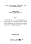
Gridding
Aero Troll uses an overset grid, also known as a Chimera, approach to gridding. In an
overset grid approach, a set of structured grids are created and linked together by
interpolation coefficients which pass information from one grid to another. An overset
grid for a multi element airfoil is shown below. The multi element airfoil is the final
example of this manual.
In the image above, four grids are visible: 1) slat grid, 2) main wing grid, 3) flap grid, and
4) background Cartesian grid. The image above is the final grid product. To achieve
this, first the individual grids need to be calculated. Then, points which lie inside the
geometry of a component, or possibly close to it, are removed, or iblanked. Next,
trilinear interpolation coefficients for the fringe, i.e. edge, points are determined.
66
The following images shows the multi element airfoil grid set before the hole punching
(cutting and trimming) is done.
67
The next image shows both the cut and trimmed grid points in cyan and green
respectively. The cut points lie within the geometry (which includes a tolerance distance
(specified by the user) from the geometry edge). The trimmed points are a user specified
number of layers trimmed away from the cut edge.
68
The next image shows the fringe points in blue.
As can be seen from the image above, fringe boundaries have two layers of points. The
CFD method used by Aero Troll requires that the interpolation coefficients for the very
outer layer of fringe points always be determinable. The second layer is not required but
is beneficial. One fringe layer is required for the 2nd order flux stencil. Two fringe layers
facilitate the artificial dissipation method. The fringe points for which required
interpolation coefficients can not be found are called orphan points. In future versions of
Aero Troll, for which higher order methods may be implemented, the number of
requested fringe layers will increase.
Creating a grid set is challenging and very much of an art. Experimentation by the user is
required to become proficient at generating a grid set.
At the moment, Aero Troll has two types of grids. One type of grid fits around objects
and is called a body conforming grid. The second type is a background block grid. This
discussion will focus on the grid generation parameters for the body conforming grids.
Block grids and the other required input for the body conforming grids will be left to the
examples.
The body conforming grid is created with an implicit hyperbolic grid generator which
marches off the surface. Another type of body conforming grid generation method,
69
which is not implemented currently in Aero Troll, is an elliptical grid generator. In
general, and in contrast to elliptical grids, a hyperbolic grid is easier to set the boundaries,
is not as smooth, and can be more problematic in regards to the grid generation. When
setting up a hyperbolic grid, the user must specify the surface grid, the spacing used when
marching off the surface, and the grid generation parameters. This discussion will focus
on some of the grid generation parameters and leave the other items to the examples.
A brief overview of the following grid generation settings will be:
1)
Sub Steps
2)
Xi Volume Smoothing
3)
Xi Slope Smoothing
4)
Zeta Spread Start
5)
Zeta Spread End
6)
Average Volume Weighting
The following settings will not be discussed and it is recommended they be left at the
default settings.
1)
Metric Multiplier
2)
2nd Order Dissipation.
To help with the discussion, the slat and main wing grids will be used. These cases are
included in the examples directory.
70
The baseline slat grid from the multi element example, along with a table of the
parameter values, is shown below.
Grid
Sub Steps
Xi Volume Smoothing
Xi Slope Smoothing
Zeta Spread Start
Zeta Spread End
Average Volume Weighting
71
Slat
4
10.0
0.0
0.0%
300.0%
0.0
The baseline main wing grid from the multi element example, along with a table of the
parameter values, is shown below.
Grid
Sub Steps
Xi Volume Smoothing
Xi Slope Smoothing
Zeta Spread Start
Zeta Spread End
Average Volume Weighting
Main
1
10.0
10.0
0.0%
300.0%
0.6
Sub Steps
The number of sub steps, or sub iterations, is the number of iterations that occurs in the
zeta (off body) direction for a xi (circumferential) grid line to be drawn. In general, the
number of sub steps is 1. In other words, a grid line is drawn for each iteration. For
geometries with a lot of curvature, more sub steps may be required so oscillations do not
occur and/or zeta lines do not overshoot and cross one another. However, too many sub
iterations will cause the grid to have difficulty changing direction and thus cross.
Therefore, either too few or too many sub steps may cause the grid generation process to
fail.
72
The slat grid will be used as an example. If the number of sub steps is set to 1, then the
gridding will blow up and a solution is not found.
Two sub steps results in the following grid.
Grid
Sub Steps
Xi Volume Smoothing
Xi Slope Smoothing
Zeta Spread Start
Zeta Spread End
Average Volume Weighting
73
Slat
2
10.0
0.0
0.0%
300.0%
0.0
Ten sub steps results in the following grid.
Grid
Sub Steps
Xi Volume Smoothing
Xi Slope Smoothing
Zeta Spread Start
Zeta Spread End
Average Volume Weighting
Slat
10
10.0
0.0
0.0%
300.0%
0.0
Notice the higher amount of sub steps forces the zeta grid lines from the sharp lip and the
trailing edge to squeeze together and attempt to intercept one another.
74
To get a better idea what occurs when the number of sub steps is set to one, the off body
(zeta) marching length will be reduced. This is shown below.
Grid
Sub Steps
Xi Volume Smoothing
Xi Slope Smoothing
Zeta Spread Start
Zeta Spread End
Average Volume Weighting
Slat
1
10.0
0.0
0.0%
300.0%
0.0
As can be seen, the poor grid accuracy causes an oscillation to build.
Xi Volume and Slope
Because the grid generator for Aero Troll is an implicit method, the entire grid is
marched forward by coupling together all the grid points on a xi surface. In other wards,
a point on a grid surface is marched to the next position by not only taking into account
its normal vector, but also taking into account changes in the surrounding normal vectors.
This is different than an explicit marching method which only accounts for the grid point
normal vector and neglects changes caused by marching forward the surrounding grid
point normal vectors and neglects what is occurring in the region of that point. Using an
implicit method opens up the opportunity to change how the surrounding normal vectors
75
feedback to the normal vector of a grid point. This is where Xi Volume and Xi Slope
come in. Setting these parameters to a value greater than zero will overemphasize how
changes in a region affect the points of that region as they are marched forward. For
example, if a cluster of points are trying to come together, thus shrinking the cell
volumes, a positive value of Xi Volume will push the points apart. On the other hand, if
the points are trying to spread apart, then a positive value of Xi Volume will pull together
the points. In the same sense, if a set of zeta grid lines are trying to curve in a certain
direction, positive values of Xi Slope will push the lines in the other direction.
A value of zero for either Xi Volume or Xi Slope indicts a modification to the feedback
does not occur for that parameter.
In general, Xi Volume is modified first and then Xi Slope. The gridding process seems to
be, in general, more robust for changes in Xi Volume.
The following examples illustrate the process. Since a xi grid surface is created using a
coupled system, the interactions can be complex.
76
The following image is the baseline grid for the slat.
Grid
Sub Steps
Xi Volume Smoothing
Xi Slope Smoothing
Zeta Spread Start
Zeta Spread End
Average Volume Weighting
77
Main
4
10.0
0.0
0.0%
300.0%
0.0
The next images shows the result for increasing Xi Volume to 30.
Grid
Sub Steps
Xi Volume Smoothing
Xi Slope Smoothing
Zeta Spread Start
Zeta Spread End
Average Volume Weighting
Main
4
30.0
0.0
0.0%
300.0%
0.0
Notice that the grid lines emanating from the bottom slat surface between the lip and
trailing edge are resisting being clumped together. Also notice that the grid lines at the
trailing edge on the top side are resisting being pulled apart.
78
The following image shows the main wing cavity for Xi Volume of 5.
Grid
Sub Steps
Xi Volume Smoothing
Xi Slope Smoothing
Zeta Spread Start
Zeta Spread End
Average Volume Weighting
Main
1
5.0
0.0
0.0%
300.0%
0.6
The red dots above indicate that negative volumes, i.e. Jacobians, have occurred.
79
The following image shows the main wing cavity for Xi Volume of 10.
Grid
Sub Steps
Xi Volume Smoothing
Xi Slope Smoothing
Zeta Spread Start
Zeta Spread End
Average Volume Weighting
80
Main
1
10.0
0.0
0.0%
300.0%
0.6
As can be seen in the above image, the lines have been forced apart, however the lines
are still sloppy in regards to the slope. To correct this, Xi Slope will be increased to 10.
Grid
Sub Steps
Xi Volume Smoothing
Xi Slope Smoothing
Zeta Spread Start
Zeta Spread End
Average Volume Weighting
81
Main
1
10.0
10.0
0.0%
300.0%
0.6
The next image shows what occurs at the leading edge of the main element when Xi
Slope is increased to 20.
Grid
Sub Steps
Xi Volume Smoothing
Xi Slope Smoothing
Zeta Spread Start
Zeta Spread End
Average Volume Weighting
Main
1
10.0
20.0
0.0%
300.0%
0.6
Spread Start and Spread End
The spread start and end parameter allows for the user to specify how the grid spacing
between points on a xi surface changes as the grid marches away from the surface.
Spread end is a means by which the grid is forced to have equidistant spacing between
the grid points at some distance from the surface. For example, if the value is set at
300% then at 3x the specified maximum off surface distance the grid is assumed to have
equal spacing between grid points. If the value was 100%, then the last grid xi grid
surface would have equal spacing. The spread start value specifies the point at which
point redistribution starts. The amount of point redistribution which occurs is a weighted
average that is a function of the distance between the start and end. For example, if the
zeta distance is half way between the start and end, then the requested distance between
82
points is influenced by weighted average between 50% of the current xi grid spacing and
50% of the average xi grid spacing. If both the spread start and end are set to zero then
spacing redistribution does not occur.
The following example shows the slat grid if the Spread End distance is 0%.
Grid
Sub Steps
Xi Volume Smoothing
Xi Slope Smoothing
Zeta Spread Start
Zeta Spread End
Average Volume Weighting
83
Slat
4
10.0
0.0
0.0%
0.0%
0.0
The following example shows the slat grid if the Spread End distance is 200%.
Grid
Sub Steps
Xi Volume Smoothing
Xi Slope Smoothing
Zeta Spread Start
Zeta Spread End
Average Volume Weighting
As can be seen, the grid lines spread out as zeta increases.
84
Slat
4
10.0
0.0
0.0%
200.0%
0.0
The following image shows the effects of changing the zeta spread start value. As can be
seen, the spreading of the grid lines is delayed until off the surface by an amount.
Grid
Sub Steps
Xi Volume Smoothing
Xi Slope Smoothing
Zeta Spread Start
Zeta Spread End
Average Volume Weighting
Slat
4
10.0
0.0
25.0%
200.0%
0.0
Average Volume Weighting
The final parameter to be discussed is an average volume weighting. The value specifies
the amount of the current versus neighboring values to use. It is a means of smoothing
out the volume in local areas where the volume is a strong function of xi. This value is
different than the Xi Volume parameter in the sense that it is more localized and is a
function of the actual volume at a given xi grid line rather than changes which occur as
the grid marches out. In other words, it is a parameter which affects the explicit rather
than implicit behavior. A value of zero for the average volume weighting signifies that
adjacent volumes should not be weighted into the volume calculation.
85
The following image shows the cavity grid using an average volume weighting of 0.0.
Grid
Sub Steps
Xi Volume Smoothing
Xi Slope Smoothing
Zeta Spread Start
Zeta Spread End
Average Volume Weighting
86
Main
1
10.0
10.0
0.0%
300.0%
0.0
The following image shows the cavity grid using an average volume weighting of 0.6.
Grid
Sub Steps
Xi Volume Smoothing
Xi Slope Smoothing
Zeta Spread Start
Zeta Spread End
Average Volume Weighting
Main
1
10.0
10.0
0.0%
300.0%
0.6
CFD Execution Settings
The following section gives a brief description of some CFD parameters used in the
following examples. They will be described again when the CFD components are
described.
B.C. Settings
Before a CFD job can be executed, the boundary conditions must be specified. Listed
below are possible choices. Not all choices are available for every circumstance.
87
Far Field Boundaries
Freestream:
The Freestream boundary condition will explicitly set the
boundary to the freestream values.
Characteristic:
The Characteristic boundary condition uses the Reimann
variables determined from the freestream and the point just interior to the
boundary to determine the values at the boundary. The Reimann variables
are based on a wave equation representation of the Euler equations.
Waves can travel from the interior points out the boundary and from the
outside (freestream) into the interior. Based on this, the values at the
boundary are determined. In general, this is the preferred far field
boundary condition.
Inlet/Outlet:
The Inlet/Outlet boundary condition sets the boundary
value to either the freestream or to the point just interior to the boundary
depending on the direction of the velocity vector. If the flow is coming
into the boundary then the boundary is set to the freestream value. If the
flow is exiting the boundary then the boundary is set to the flow values of
the point just interior to the boundary.
Fringe:
The Fringe boundary condition specifies that the far field
boundary for the grid is a fringe boundary and must interpolate the values
from another grid.
Surface Boundaries
Auto:
The Auto boundary condition will set the surface to a slip
boundary condition if the Euler equations are being used or to a no-slip
boundary condition if the Navier Stokes equations are being used. Two
boundary sub types are available. The Momentum sub type specifies that
the momentum equations should be used to determine the flow values at
the surface. This should be selected if the off body spacing is large. The
Extrapolate sub type specifies that the flow values should be extrapolated
from the values off the surface. This sub type should be used if the off
body spacing is small. In general, the Extrapolate boundary condition is
used for the Navier Stokes equations since the off body spacing tends to
be very small.
Slip:
The Slip boundary condition specifies that the velocity at
the surface is not zero. Two boundary sub types are available; 1)
Extrapolate and 2) Momentum. These are described in the Auto boundary
condition description above.
No Slip:
The No Slip boundary condition specifies that the velocity
at the surface is zero. Two boundary sub types are available; 1)
Extrapolate and 2) Momentum. These are described in the Auto boundary
condition description above.
Time Stepping Values
There are two approaches to marching a solution forward: 1) global time stepping (dt),
and 2) local time stepping, (CFL). The global time stepping approach marches all the
88
grid points forward in time by a uniform constant time step. This method is a time
accurate method. The local time step will vary the time step for a grid point by the
volume associated with that grid point. The larger the volume, the large the time step is.
This method is not a time accurate method. The advantage of local time stepping is that
it accelerates the convergence to steady state. It must be noted that the global and local
time stepping approach may not necessarily converge on the same steady state solution
since the equations for time are different between the two approaches. If the two
methods give different solutions, then the time accurate approach is the physically correct
method. However, frequently, the two approaches do converge on the same solution.
The screen capture below shows example settings for global time stepping approach. For
this set of input, the user specifies the global time step, dt. The user can also set a low
and a high bracketing value for the CFL number. Setting the CFL min or CFL max
value to zero specifies that the low and/or high bracketing value is not used.
The screen capture below shows example settings for local time stepping approach. For
this set of input, the user specifies the local time step, CFL. The user can also set a low
and a high bracketing value for the dt number. Setting the dt min or dt max value to
zero specifies that the low and/or high bracketing value is not used.
CFD Display Settings
The following section describes the settings to modify the interval at which solution
parameters are shown.
Resid Iterations:
The interval at which the CFD residuals and
solution deltas are passed to Aero Troll execution dialog.
Force Iterations:
The interval at which the loads integrated by the
CFD execution module are passed to the Aero Troll execution dialog.
89
Update Iterations:
The interval at which the Main Window contour
plot is updated.
Size of Max. Resid Pts:
The size of the points in pixels which identifies the
grid point location of the maximum residual.
# of Max. Resid Pts:
The number of iterations for which the location of
the maximum residual is identified.
Size of Marked Pts:
The default size of the points in pixels which
identifies cut, trimmed, boundary, fringe, upgraded, and orphan point.
Plotting Contours
The Plot menu for the main Aero Troll window allows for the user to select the contour
type. The majority of contour types are non-dimensional. The following list shows the
name of the contour type and how the value is non-dimensionalized. The contour values
available from the menu will depend on the analysis components created and setup for
the analysis.
Mach:
Local velocity magnitude non-dimensionalized by the local speed
of sound.
Velocity:
Local velocity non-dimensionalized by the freestream speed of
sound.
p/p_inf:
Pressure non-dimensionalized by the freestream pressure.
d/d_inf:
Density non-dimensionalized by the freestream density.
T/T_inf:
Temperature non-dimensionalized by the freestream temperature.
Cp:
The coefficient of pressure.
entropy:
The difference of the local entropy and the freestream entropy.
Entropy is non-dimensionalized by the ratio of the gas constant to the ratio
of the specific heats subtracted by one (R∞/[γ-1]).
enthalpy:
The difference of the local total enthalpy and the freestream total
enthalpy non-dimensionalized by the square of the speed of sound.
viscosity (μ): Local molecular viscosity non-dimensionalized by the freestream
molecular viscosity .
eddy μ ratio: Local eddy viscosity non-dimensionalized by the freestream
molecular viscosity.
vorticity:
.Local vorticity non-dimensionalized by the freestream speed of
sound.
90
dq: .
The L2 norm, |dq|, of the local solution vector.
dt:
The local time step.
CFL:
The local Courant–Friedrichs–Lewy number.
distance:
The distance to the nearest surface in grid units. This value is
dimensional.
MDADI metric: A metric used to determine if the diagonalized ADI or ADI
method should be used for a grid line.
The plot menu also allows the user to set the min and max values for the current contour
and also show and hide the contour plot key. To remove a min/max constraint, clear the
field and leave it blank.
WEDGE
The purpose of this example is to demonstrate the analysis of a simple arbitrary body
made up of line segments and the use of multiple overlapping grids. The Reynolds
number based on the chord length of 2 is 1.0E7. Using the y+ tool, as demonstrated by
the NACA 0012 example, indicates that setting the off surface spacing to 2.0E-6 is
reasonable for a y+ value of 1.
91
As with the previous examples, start Aero Troll and add an Analysis component. Next,
add an airfoil component and name it Wedge. The main window appears as follows.
92
Problem Specification
Geometry Setup
The next few steps will define the 2D geometry for the wedge. The geometry MUST be
defined in a clockwise fashion. The geometry definition will start at the trailing edge and
loop around to the bottom middle, to the leading edge, to the top middle, and then back to
the trailing edge. The wedge is 20% thick and the maximum thickness is located at 50%
of the chord. The chord length is 2. To start the process of creating the wedge geometry,
open the edit panel for the Wedge component, select the User Defined radio button, and
set Start Pt to x=2.0 and y=0.0. The start point is the first point of the mold line which
describes the geometry and, for this example, the point is the trailing edge.
93
Next, right click in the User Defined Mold Line list to display the segment pop-up menu
and select the Add Segment menu item.
The segment selection window will appear. Select Line and then press the OK button.
94
The line input window will appear.
Set the end point of the line to x=1.0 and y=-.2. And then select the OK button.
Create three additional lines by repeating the process above. Each new line segment
should be added below the previous one by right clicking in the region of the User
Defined Mold Line list below the previously added line segment. The end points for
each line are shown in the table below.
x
0.0
1.0
2.0
y
0.0
0.2
0.0
95
Once the lines have been created, the main window will look as follows.
96
Because of the geometry of the wedge, an H grid will be used. Unlike a C or an O grid,
an H grid will need to know where both the leading and trailing edge are. The trailing
edge is automatically set to the location of the start point. However, the leading edge
needs to be specified. Right click on the second line segment and select the Set LE
Below menu item. A warning concerning point distributions will appear. Select the Yes
button. The leading edge will be positioned at the end point of the second segment.
97
The edit panel will now look as follows. Notice the yellow leading edge line has moved
to a position below the second line segment
98
The next step is to set the number of surface points for each line segment to 101. Start by
right clicking on the first line segment and selecting the Edit Points menu item. Unlike
the NACA 0012 example, the point distribution will be kept at constant spacing intervals
to simplify this example. For a true run, the points should be clustered at the four wedge
apexes. This will be left for the user to experiment with separately from this example.
99
Set the number of points to 101 and select the OK button.
In a similar fashion, set the number of points for all the line segments to 101.
100
Initial CFD Setup
The next step in the process is to add the CFD components and make the required
connections. Start the process by creating an AT_Airfoil_CFD component and naming it
Wedge CFD. To do this, right on the AT Analysis component and select the
At_Airfoil_CFD component from the Add menu. Name the component Wedge CFD.
101
Next, create a CFD Grid Group for the Wedge CFD component by right clicking on
Wedge CFD component and selecting the CFD Grid Group component from the Add
menu. Set the name of the CFD Grid Group to Wedge Grid Group.
102
The Wedge Grid Group will define the wedge near body grid. The far field grid will be
created using a 2D block grid. Right click on the Wedge CFD component and select the
CFD 2D Block Grid menu item from the Add menu. Name the CFD 2D Block Grid to
Wedge Block Grid.
103
The next step is to link the Wedge CFD method to the wedge. Link the Wedge CFD
component to the wedge component by clicking and holding the left mouse button while
over the Wedge CFD component and then dragging and dropping the Wedge CFD on to
the wedge component.
104
Now that the Wedge CFD method and wedge are linked, the wedge component can be
linked to the Wedge Grid Group. To accomplish this, click and hold the left mouse
button while over the wedge component belonging to the Wedge CFD component, and
then drag and drop the component on to the Wedge Grid Group component. For this to
work, the wedge component under the Wedge CFD component, and not the wedge
component under the AT Analysis component, must be used.
105
Before an analysis is performed, the analysis methodology for the wedge component
must be chosen. To select the analysis method for the wedge component, right click on
the wedge component node in the components tree to show the component popup menu
and then select the Wedge CFD method under the Analysis Type submenu.
106
CFD Gridding
Now that the initial setup is done, a CFD grid must be built for the wedge and the far
field. To start this process, open the edit panel for the Wedge Grid Group by right
clicking on it and selecting the Edit menu item.
107
The edit panel for the Wedge Grid Group will be displayed.
108
The first step in the process of defining a grid is to specify the surface grid. For this
example, the forward and aft length of the H grid will be kept at 1.0. The forward length
is the length of the forward segment which connects to the leading edge. The aft length is
the length of the aft segment which connects to the trailing edge. In general, if they are
being used, the aft and forward segment length would be modified.
Right click on Aft Segment in surface grid segment list.
109
The edit window for the segment will appear. Set the number of points to 51 and
Beginning Connection to connect and Ending Connection to float. Then select the OK
button.
The segments which define the geometry are laid out in clockwise fashion so the
beginning and end of a segment is representative of that. In the case of the aft segment,
one must think of it as being attached to the geometry after the clockwise traverse is
made. Therefore the beginning of the aft segment is attached to the end of the last
geometry segment. In a similar way, the end of the forward segment is attached to the
leading edge.
By setting the aft segment beginning connection to connect, an attempt will be made to
smoothly transition the grid spacing from one segment, in this case the trailing edge, to
another, in this case the beginning of the aft segment. For the case of aft segment, the
trailing edge grid spacing is determined by averaging the grid spacing of the top and
bottom surface at the trailing edge.
Next, open the edit dialog for the first line segment. Set the number of points to 51 and
both the beginning and ending connections to “Delta % of Avg” and a value of 10%.
Then select OK. This specifies that the grid spacing at the beginning and end of the
110
segment is equal to 10% of the average spacing. Therefore, points will be clustered at the
beginning and end.
Repeat the process for each of the wedge segments.
111
For the forward segment, set the number of points to 51, the beginning connection to
float, and the ending connection to connect. The grid point spacing settings are the
mirror image of the aft segment grid point spacing settings.
112
The next step is to set the top level parameters for the volume grid. Set the Beginning
Grid B.C. to Float and set Xi Volume Smoothing to 20.
113
Next right click on the Geometric(S):[0] zeta grid segment and select the Edit Zeta
Segment menu item.
114
Then set the length to 0.8, the number of points to 151, set the first grid spacing, ds[0], to
1.0E-6, and select the OK button.
115
Finally, set Surface B.C. to Auto and the Farfield B.C. to Fringe. A fringe setting
indicates to the system that the grid points at that boundary will get their values from
another grid, in this case the far field grid.
116
Next, calculate the grid. Select the Calculate Grid menu item from the Commands
menu.
117
The main window will look as follows.
118
Next, set up the Wedge Grid Block. The block grid is a Cartesian grid with constant
spacing. Open the edit panel for the Wedge Grid Block by right clicking on it and
selecting the Edit menu item.
119
The edit panel for the Wedge Grid Block will be displayed.
The overall procedure is to specify the horizontal (Xi) grid lines and the vertical (Zeta)
grid lines. Currently four different spacing types are available: 1) Constant, 2)
Geometric(S), 3) Geometric(E), and 4) TanH. Constant grid spacing specifies that the
grid cell length is constant along a side. A Geometric(S) grid spacing specifies that the
grid cells increase in a geometric fashion and that the user sets the first, i.e. starting, grid
cell spacing. A Geometric(E) grid is similar to Geometric(S) except that the user
specifies the last, i.e. ending, grid cell spacing. The TanH grid cell spacing is identical to
that used for the surface grids and requires the user to specify how the first and last grid
cell spacing is to be handled.
For this example, both the horizontal and vertical grid lines will be set as constant. Also,
the will be reflected about both horizontally and vertically.
120
Right click on the Geometric(S):[0] segment in the Xi Grid segment list and select the
Edit Segment menu item from the popup menu.
121
The edit panel for the Xi Grid segment will be displayed.
For this example set the length to 3.0, the number of nodes to 61, and the spacing type to
constant. Then select the OK button.
122
In a similar fashion, right click on the Geometric(S):[0] segment in the Zeta Grid segment
list and select the Edit Segment menu item from the popup menu. Set the length to 3.0,
the number of nodes to 61, and the spacing type to constant. Then select the OK button.
123
Next, return back to the edit panel for Wedge Grid Block and shift the grid back by two
units by setting X Shift to 2.0, reflect the grid about the vertical and horizontal axis by
selecting the Reflect YZ and Reflect XY checkboxes, set the Outer B.C. to
characteristic, and set the Inner B.C. to Fringe.
124
Next, calculate the grid. Select the Calculate Grid menu item from the Commands
menu.
125
The main window will look as follows.
CFD Run Setup
The next step is to set up the CFD parameters. For this example the Reynolds Averaged
Navier Stokes (RANS) solver using the Spalart Allmaras turbulence model will be used.
The Left Hand Side (LHS) matrix solver for both the Xi and Zeta direction of the implicit
solver will be set to Alternating Direction Implicit (ADI). In general, the ADI method
allows for significantly larger Courant-Friedrichs-Lewy (CFL) time step for local time
stepping than the Diagonalized Alternating Direction Implicit (DADI) method for grids
defining an airfoil. The reason is that the DADI method requires an approximation of the
viscous terms in the diagonalized matrix solver. This approximation causes errors in the
wake region which reduces the allowed CFL number.
Before a CFD run can be made, Aero Troll will prepare the grids by cutting a hole into
the Grid Block grid and connecting the fringe points. In the example the fringe points
will be the outer two layers of the wedge grid and the inner two layers at the edge of the
hole that will be punched into the block grid. At this time, the hole cutting methodology
is very simple; any point which lies within the body or within an area next to the body
(buffer zone), specified by the user, is eliminated. The size of the buffer zone is specified
with the Hole Border parameter. Once the preliminary hole is punched, a number of
layers, as specified by the Trim Passes parameter, will be stripped away. That new edge
126
now becomes the edge of the hole. For this example, Hole Border will be set to 0.2 and
Trim Passes will be left at the default of 1. Determining the proper procedure for cutting
holes into grids is a trial and error process and is left, to a large degree, to the user. One
of the key points is to try to insure that one grid does not pick up boundary layer flow
values to the extent possible. The reason is that the gradients within the boundary layer
are large and the grid cell sizes of the grids do not match well.
The first step in the CFD process setup is to open the Edit Dialog for the Wedge CFD
component by right clicking on the Wedge CFD component in the component tree and
selecting the Edit menu item. Next, set the solution type to Turb (SA), the number of
iterations to 1000, the CFL number to 90, and the LHS Xi and Zeta methods to ADI.
These changes are shown below. The CFL number was determined by trail and error.
First a value of 60 was used and then increased until the maximum convergence rate was
found.
127
Next, the input screen for the Wedge CFD component will be switched to Grid and the
Hold Border parameter will be set to 0.4.
128
For this example, the Wedge CFD component display variables will be left to the default
value. The residual will be extracted every iteration, the CFD load coefficients will be
extracted every 20 iterations, and the main window contour plot will be extracted every
100 iterations. If the user chooses, changes to these values can be done in the Display
input screen for the Wedge CFD component.
129
The next step is to build the overlapping grid set by selecting the Calculate Grids menu
item from the Commands menu.
130
The main window will look as follows.
131
Various characteristics of the wedge and block can be investigated by selecting menu
items from the Points sub menu under the View menu of either the Wedge Grid Group or
the Wedge Grid Block components. For example, the fringe points for the wedge grid
can be displayed by selecting the Show Fringe menu item of the Points menu under the
View menu.
132
The main window appears as follows.
133
In a similar fashion, the fringe points for the block grid can also be displayed. The image
below shows the fringe points for both the wedge and block grids. The view was zoomed
into the wedge to see the block grid fringe points clearer.
To return back to this example, hide the fringe point display and zoom out from the view.
134
Before the CFD run can be executed, the freestream values must be set. Right click on
the AT Analysis component and select the Edit menu item.
135
The edit panel for the AT Analysis component will be displayed. Set the included angle
of attack to 4.0, the Mach number to 2.0, and the Reynolds number per length to 5E6.
The Reynolds number for the wedge based on the chord is 10E6. Therefore, since the
chord is 2.0, the Reynolds number per length is ½ the root chord Reynolds number.
Finally, sRef and lRef are set to 2.0.
136
CFD Execution
To execute the run, select the Execute menu item from the AT Analysis component
menu.
137
Once execution begins, the Exec AT CFD Dialog will be shown. To allow for cleaner
residual plots, some of the settings will need to be changed. For the Wedge Grid Group
deselect the CFL rMax, sAvg, and sMax check boxes. All that will remain checked is
CFL rAvg. This indicates that only the average CFL residual will be displayed.
138
Next, go to the Wedge Grid Block Grid Group and deselect the Include in Global Block
check box. This indicates that the Wedge Grid Block residual values will not be included
in the plot when the Plot All button is selected.
139
After a few iterations, select the Plot All button of the Wedge Grid Group Grid Group.
140
The residual plot will be shown below.
141
After a few more iterations the For+Mom tab of the Exec AT CFD Dialog is selected
and the Plot All button is selected.
142
The plot for CZ is shown below. The plot contains the curves for both the wedge and the
block. The CZ for the block is zero.
143
Once the CFD job is complete, dismiss the Exec AT CFD Dialog by selecting the Close
button.
144
To view the results after the CFD run is completed, select the Results menu item under
the AT Analysis and Wedge components. The AT Analysis results will provide the
results for the complete configuration and the Wedge results will provide more detail,
such as surface pressure and skin friction coefficients. To view the results for the Wedge,
right click on the wedge and select the Results menu item.
145
The results window will be displayed. Select the Plot button to display the wedge cp.
146
The cp plot will be displayed.
This concludes the example.
MULTI-ELEMENT Airfoil
The purpose of this example is to demonstrate the analysis of a more complex geometry
which involves multiple geometry elements. Hopefully this example will guide the way
in creating other arbitrary 2D geometries.
Problem Specification
147
As with the previous examples, start Aero Troll and add an Analysis component. Next,
add three airfoil components and name them Slat, Main, and Flap. The main window
appears as follows.
148
Slat Geometry
To start the process of creating the slat geometry, open the edit panel for the Slat
component, select the User Defined radio button, and set Start Pt to x=0.413864 and
y=0.11262594. The start point is equal to the first point of the cubic spline which will be
read in later.
149
Next, right click in the User Defined Mold Line list to display the segment pop-up menu
and select the Add Segment menu item.
The segment selection window will appear. Select Cubic Spline and then press the OK
button.
150
The cubic spline input window will appear.
Input fields for the
cubic spline input
table.
151
Right click on an input field for the cubic spline input table to display the cubic spline
pop-up menu, select the Open menu item, and open the 30P-30NCoord_slat_A.dat file
which can be found in the MD_30P_30N example folder.
152
The window will appear as follows.
153
Select the OK button to accept the input. Next, right click in the User Defined Mold
Line list below the previously added cubic spline segment and add a new cubic spline.
For this example, the new cubic spline must be added below the previously added cubic
spline.
Then insert the 30P-30NCoord_slat_B.dat file into the new cubic spline following the
same process outlined above.
154
The main window now appears as follows.
modified later.
155
The coarse outline of the slat will be
The next step is to add an elliptical arc segment between the end of the first cubic spline
and the beginning of the second cubic spline. To do this, right click on the second cubic
spline segment and select the Add Segment menu item. This will add a segment in the
position selected and push down the segment which occupies the slot.
Select an Elliptical Arc and then select the OK button.
156
When the elliptical arc edit window appears set the End Pt. to x=-0.575833
y=-2.37736857 and set both the Start and End slope to Connect. Then select the OK
button.
157
Next, set the number of points for the first cubic spline to 101 by right clicking on the
first cubic spline and selecting the Edit Points menu item.
158
Set the number of points to 101 and select the OK button.
159
In a similar fashion, set the number of points on the elliptical arc to 11 and the number of
points on the second cubic spline to 101. The main window will look similar to the
following image.
160
Main Geometry
To start the process of creating the main geometry, open the edit panel for the Main
component, select the User Defined radio button, and set Start Pt to x=19.2256548
y=0.6740228.
161
Next, right click on the User Defined Mold Line list to display the segment pop-up
menu and select the Add Segment menu time.
The segment selection window will appear. Select the Cubic Spline and then press the
OK button.
162
The cubic spline input window will appear.
163
Right click on an input field for the cubic spline input table to display the cubic spline
pop-up menu, select the Open menu item, and open the 30P-30NCoord_main_A.dat file.
164
The window will appear as follows.
165
Select the OK button to accept the input. Next, right click in the User Defined Mold
Line list below the previously added cubic spline segment and add a line segment. For
this example, the line segment must be added below the previously added cubic spline.
166
Set the line end point to x=15.4, y=-0.378928, then select the OK button to accept the
input. Next, right click in the User Defined Mold Line list below the previously added
line segment and add a new cubic spline. For this example, the new cubic spline must be
added below the line segment.
Then insert the 30P-30NCoord_main_B.dat file into the new cubic spline following the
same process outlined above for the first cubic spline.
167
The main window will now look as follows.
For the main airfoil body, set the number of points of the first cubic spline to 21 points
and set the number of points on the line to 21 points.
168
The next step is to split the last cubic spline by adding a break at the leading edge. To
create the break, the surface length from the beginning of the cubic spline to the leading
edge must be determined. First select the Mold Line menu item from the Plot menu of
the main airfoil component edit panel.
169
The segment display for the main airfoil will appear. Select the Show Cntrl Pts menu
item of the Segment Display’s View menu.
170
Then zoom into the leading edge by using the middle mouse button to zoom and the left
mouse button to translate right/left and up/down. The Segment Display window will look
similar to the figure below.
171
Double click on the control point at the leading edge. The point to click on is shown
below. A Point Display window containing the information for that point will appear.
The Point Display window contains the x, y, and z coordinates for the control point. The
window also contains the distance along the surface from the beginning of the segment to
the control point. This distance is approximately 14.695. It should be noted that the
Point Display window will only appear when a control point is double clicked. Double
clicking anywhere else on the segment will not display information about the clicked
location. Next, close the Point Display and Segment Display windows by selecting the X
in the upper right hand corner of the window frame for both windows.
172
The next step is to create a break at the leading edge. Right click on the second cubic
spline in the Main airfoil edit panel and select the Add Break menu item.
The add break window will appear. Set the number of points to 101, the segment length
to 14.695, and then select the OK button.
173
Next, right click on the last segment of the second cubic spline, Cubic Spline[1], and
select the Edit Points menu item. Then set the number of points to 101 and select the
OK button.
174
The main window will appear as follows.
175
Flap Geometry
To start the process of creating the flap geometry, open the edit panel for the Flap
component, select the User Defined radio button, and set Start Pt to x=24.81195666,
y=-3.21197394.
176
Next, right click on the User Defined Mold Line list to display the segment pop-up
menu and select the Add Segment menu time.
The segment selection window will appear. Select the Cubic Spline and then press the
OK button.
177
The cubic spline input window will appear.
178
Right click on the cubic spline input table to display the cubic spline pop-up menu, select
the Open menu item, and open the 30P-30NCoord_flap.dat file.
179
The window will appear as follows.
Next, find the leading edge surface distance for the flap using the same method as
outlined in the main airfoil section. For the flap, the surface distance to the leading edge
is 6.8576. Then, as with the main airfoil, create a break at this location and set the
number of points for both the top and bottom segment to 101.
180
The main window will look as follows.
181
Initial CFD Setup
The next step in the process is to add the CFD components and make the required
connections. The process is similar to that described for the NACA 0012 and Wedge
example. Start the process by creating an AT_Airfoil_CFD component and naming it
MD_30P_30N. Next, create three CFD Grid Groups for the MD_30P_30N and name
them Slat Grid Group, Main Grid Group, and Flap Grid Group. Next, add two CFD 2D
Grid Block components to the MD_30P_30N. Name the first one Near Block Grid and
the second one Far Block Grid. The main window should look like the following figure.
182
The next step is to link the MD_30P_30N method to the slat, main, and flap elements of
the multi-element airfoil. Link the MD_30P_30N component to the slat component by
clicking and holding the left mouse button while over the MD_30P_30N component and
then dragging and dropping the MD_30P_30N on to the slat component. Repeat the
process for the main and flap elements. The main window should look like the following
figure.
183
Now that the MD_30P_30N method and elements are linked, the element components
can be linked to the grid groups. To accomplish this, click and hold the left mouse button
while over an element component, which is attached to the MD_30P_30N component,
and then drag and drop the component on to the grid group component. For this to work,
the element component under the MD_30P_30N component, and not the element
component under the AT Analysis component, must be clicked on. The main window
should look like the following figure.
Before an analysis is performed, the analysis methodology for the element components
must be chosen. To select the analysis method for the element components, right click on
an element component node in the components tree to show the component popup menu
and then select the MD_30P_30N method under the Analysis Type submenu.
CFD Gridding
Now that the geometry setup is completed, CFD grids must be built for the slat, main,
and flap elements.
The process for setting the Main Grid Group parameters will be demonstrated first. The
Main Grid Group core parameters requiring changes are shown below.
184
Main Grid Group Core Parameters
Grid Type:
Aft length:
Beginning Grid B.C.:
End Grid B.C.:
Xi Volume Smoothing:
Xi Slope Smoothing:
Zeta Spread End:
Avg. Volume Weighting
Surface B.C.:
Farfield B.C.:
C grid
13
Float
Float
10.0
10.0
300.0
0.6
Auto
Fringe
185
Open the edit panel for the Main Grid Group and make the changes shown above. The
following two figures identify the fields which need to be changed.
186
187
Next, create a break in the second cubic spline segment at the position shown below, and
set the number of points to 76.
Main Grid Group Segment Breaks
Second “Main::Cubic Spline” Segment
# of Points
S
76
14.695
Next, modify the zeta grid segment using the following values.
188
Main Grid Group Zeta Grid Parameters
Length:
Number of nodes:
Zeta Spacing Type:
ds[0]:
2.2
76
Geometric(S)
5.0E-5
189
Next, modify the surface grid segments.
Main Grid Group Segment Parameters
Aft Segment
# of Points:
Beginning Connection:
Ending Connection:
Cubic Spline Segment
# of Points:
Beginning Connection:
Ending Connection:
Line Segment
# of Points:
Beginning Connection:
Ending Connection:
Cubic Spline[0] Segment
# of Points:
Beginning Connection:
Ending Connection:
Cubic Spline[1] Segment
# of Points:
Beginning Connection:
Ending Connection:
Base Segment
# of Points:
Beginning Connection:
Ending Connection:
31
Connect
Float
21
Delta S=0.02
Connect
6
Float
Float
76
Connect
Delta S=0.005
101
Connect
Delta S=0.02
11
Delta S=5.0E-5
Delta S=5.0E-5
190
Start with the Aft Segment.
191
The following figure shows the input window for the Aft Segment.
The following figure shows the input window for Main::Cubic Spline.
192
The following figure shows the input window for Main::Line.
The following figure shows the input window for Main::Cubic Spline[0].
193
The following figure shows the input window for Main::Cubic Spline[1].
The following figure shows the input window for Main::Top Base.
194
Next, calculate the grid.
195
The grid is shown in the following image of the main window.
The next step is to set up the Slat Grid Group. The process is very similar to the set up of
the Main Grid Group. Only the parameters which require changing are shown below.
Note that the field entries Sub Steps and Avg. Vol. Weighting for the Slat Grid Group
Core Parameters are different than the Main Grid Group.
Slat Grid Group Core Parameters
Grid Type:
Aft length:
Beginning Grid B.C.:
End Grid B.C.:
Sub Steps:
Xi Volume Smoothing:
Xi Slope Smoothing:
Zeta Spread End:
Surface B.C.:
Farfield B.C.:
C grid
2.0
Float
Float
4
10.0
0.0
300.0
Auto
Fringe
196
Slat Grid Group Zeta Grid Parameters:
Length:
Number of nodes:
Zeta Spacing Type:
ds[0]:
2.2
76
Geometric(S)
5.0E-5
Slat Grid Group Segment Parameters
Aft Segment
# of Points:
Beginning Connection:
Ending Connection:
Cubic Spline Segment
# of Points:
Beginning Connection
Ending Connection
Elliptic Segment
# of Points:
Beginning Connection
Ending Connection
Cubic Spline Segment
# of Points:
Beginning Connection
Ending Connection
Base Segment
# of Points:
Beginning Connection
Ending Connection
26
Connect
Float
51
Delta S=0.003
Connect
11
Float
Float
76
Connect
Delta S=0.003
11
Delta S=5.0E-5
Delta S=5.0E-5
197
After setting the parameters for the Slat Grid Group, calculate the grid. The grid is
shown in the following image of the main window.
Next, set up the Flap Grid Group.
Flap Grid Group Core Parameters
Grid Type:
Aft length:
Beginning Grid B.C.:
End Grid B.C.:
Sub Steps:
Xi Volume Smoothing:
Xi Slope Smoothing:
Zeta Spread End:
Surface B.C.:
Farfield B.C.:
C grid
8
Float
Float
1
10.0
0.0
300.0
Auto
Fringe
Flap Grid Group Segment Breaks
Flap::Cubic Spline
# of Points
S
76
6.8576
198
Flap Grid Group Zeta Grid Parameters
Length:
Number of nodes:
Zeta Spacing Type:
ds[0]:
2.2
76
Geometric(S)
5.0E-5
Flap Grid Group Segment Parameters
Aft Segment
# of Points:
Beginning Connection:
Ending Connection:
Cubic Spline[0] Segment
# of Points:
Beginning Connection:
Ending Connection:
Cubic Spline[1] Segment
# of Points:
Beginning Connection:
Ending Connection:
Base Segment
# of Points:
Beginning Connection:
Ending Connection:
21
Connect
Float
76
Delta S=0.006
Delta S=0.006
76
Delta S=0.006
Delta S=0.006
21
Delta S=5.0E-5
Delta S=5.0E-5
199
After setting the parameters for the Flap Grid Group, calculate the grid. The grid is
shown in the following image of the main window.
Next, set up the Near Block Grid. The setup is similar to that of the Wedge example.
The Near Block Grid is comprised of two grid zones, an inner zone and an outer zone.
200
The following changes need to be made to the Near Block Grid and they are outlined in
the screen capture that follows.
Near Block Grid Core Parameters
X Shift
Z Shift
Reflect YZ Plane
Reflect XY Plane
Outer B.C.
Inner B.C.
13.0
-1.0
true
true
Fringe
Fringe
201
The next step is to create a grid segment for both the Xi and Zeta grid edges. To do this,
right click on the Geometric(S):[0] segment in the Xi Grid list and select the Add
Segment menu time. This is shown below.
202
Edit the first Xi Grid segment by right clicking on Geometric(S):[0] segment and
selecting the Edit Segment menu item.
203
The edit window for the segment will appear. Make the following changes.
Xi Grid Segment Parameters
First Segment
Length:
Number of Nodes:
Z Spacing Type:
17.0
44
Constant
204
Next, edit the second Xi Grid Segment and make the following changes.
Xi Grid Segment Parameters
Second Segment
Length:
Number of Nodes:
Z Spacing Type:
ds[0]:
30.0
26
Geometric(S)
Connect
Next, add a second segment to the Zeta Grid list and make the following changes.
Zeta Grid Segment Parameters
First Segment
Length:
4.0
Number of Nodes:
11
Z Spacing Type:
Constant
Second Segment
Length:
30.0
Number of Nodes:
26
Z Spacing Type:
Geometric(S)
ds[0]:
Connect
205
Next, calculate the grid.
206
The main window will appear as follows.
Next, set up the Far Block Grid. The setup is similar to that of the Near Block Grid. The
Far Block Grid is comprised of two grid zones, an inner zone and an outer zone. Unlike
the Near Block Grid, the inner zone for the Far Block Grid will be deactivated to make a
hole for the Near Block Grid.
207
The following changes need to be made to the Far Block Grid and they are outlined in the
screen capture that follows.
Far Block Grid Core Parameters
X Shift
Z Shift
Reflect YZ Plane
Reflect XY Plane
Outer B.C.
Inner B.C.
13.0
-1.0
true
true
Characteristic
Fringe
208
The next step is to create a grid segment for both the Xi and Zeta grid edges. To do this,
right click on the Geometric(S):[0] segment in the Xi Grid list and select the Add
Segment menu time. This is shown below.
209
Edit the first Xi Grid segment by right clicking on Geometric(S):[0] segment and
selecting the Edit Segment menu item.
210
The edit window for the segment will appear. Make the following changes.
Xi Grid Segment Parameters
First Segment
Length:
Number of Nodes:
Z Spacing Type:
42.0
22
Constant
211
Next, edit the second Xi Grid Segment and make the following changes.
Xi Grid Segment Parameters
Second Segment
Length:
Number of Nodes:
Z Spacing Type:
ds[0]:
2000.0
31
Geometric(S)
Connect
Next, add a second segment to the Zeta Grid list and make the following changes.
Zeta Grid Segment Parameters
First Segment
Length:
30.0
Number of Nodes:
16
Z Spacing Type:
Constant
Second Segment
Length:
2000.0
Number of Nodes:
31
Z Spacing Type:
Geometric(S)
ds[0]:
Connect
212
Next, deactivate the inner zone by right clicking on the Constant Xi and Zeta segments
and selecting the Deactivate menu item.
213
Next, calculate the grid.
214
The main window will appear as follows.
215
CFD Run Setup
The next step is to make changes to the MD_30P_30N component. The following
changes will be made.
MD_30P_30N
Solution Type:
Iterations:
Time Stepping :
CFL:
LHS xi:
LHS zeta:
Turb (SA)
2500
CFL
60
ADI
ADI
216
Next cut the grid holes and link the grid together by selecting Calculate Grids menu
item under the Commands menu. Note that if the grids were not previously calculated
under the various Grid Groups, the grids would be calculated at this time. Then use the
mouse to zoom closer to the multi element airfoil. The main window should appear
somewhat close to the following image.
217
The final step before running the CFD analysis is to modify the AT Analysis component.
The Reynolds number for this example is 9e6 based on the non extended (slat and flaps
not deployed) chord length of 22. Therefore, the Reynolds number per length is 9e6
divided by 22 which equals 409090.9.
AT Analysis
AlphaC
Mach
Re per len
sRef
lRef
xMom
8.1
0.2
409090.9
22.0
22.0
5.5
218
CFD Execution
Under the AT Analysis menu, select the Execute menu item.
The next series of steps will reduce the number of residuals which are plotted. The
objective is to plot only the maximum solution change for the slat, main, and flap
element. The residuals for the near and far block will be disabled to make the residual
display for this example simple. However, in general, a residual should be included for
each grid to ensure that they all converge.
219
To modify the slat residual, select the Slat Grid Group from the Grid Group drop down
menu in the Exec AT CFD Dialog. Then deselect the CFL rAvg, CFL rMax, and sMax
check boxes.
220
Repeat the process for the Main Grid Group and the Flap Grid Group.
221
222
For the near and far blocks, deselect the Include in Global Plot check box. Deselecting
this check box will specify that the residuals should not be included in the residual plot
when the Plot All button is selected.
223
224
Finally, to plot the residuals, return to the slat grid group and select Plot All button.
225
The residual plot will be shown.
After the 2500 iterations are complete, the results are as follows.
Total Results
CX
CY
CZ
Cl
Cm
Cn
CD
CL
Total
-3.91199E-01
0.00000E+00
3.17961E+00
0.00000E+00
-5.98276E-01
0.00000E+00
6.07147E-02
3.20301E+00
Pressure
-4.01123E-01
0.00000E+00
3.17757E+00
0.00000E+00
-5.99620E-01
0.00000E+00
5.06015E-02
3.20239E+00
226
Friction
9.92490E-03
0.00000E+00
2.03897E-03
0.00000E+00
1.34428E-03
0.00000E+00
1.01132E-02
6.20199E-04
Slat
CX
CY
CZ
Cl
Cm
Cn
CD
CL
Total
-2.24704E-01
0.00000E+00
2.51505E-01
0.00000E+00
8.44135E-02
0.00000E+00
-1.87025E-01
2.80657E-01
CX
CY
CZ
Cl
Cm
Cn
CD
CL
Total
-3.87818E-01
0.00000E+00
2.42860E+00
0.00000E+00
-3.18482E-01
0.00000E+00
-4.17563E-02
2.45901E+00
Pressure
-2.25736E-01
0.00000E+00
2.50403E-01
0.00000E+00
8.41257E-02
0.00000E+00
-1.88202E-01
2.79711E-01
Friction
1.03239E-03
0.00000E+00
1.10182E-03
0.00000E+00
2.87767E-04
0.00000E+00
1.17734E-03
9.45366E-04
Main
Pressure
-3.94743E-01
0.00000E+00
2.42708E+00
0.00000E+00
-3.19109E-01
0.00000E+00
-4.88260E-02
2.45849E+00
Friction
6.92523E-03
0.00000E+00
1.51560E-03
0.00000E+00
6.27026E-04
0.00000E+00
7.06969E-03
5.24703E-04
Flap
CX
CY
CZ
Cl
Cm
Cn
CD
CL
Total
2.21323E-01
0.00000E+00
4.99505E-01
0.00000E+00
-3.64207E-01
0.00000E+00
2.89496E-01
4.63337E-01
Pressure
2.19356E-01
0.00000E+00
5.00084E-01
0.00000E+00
-3.64637E-01
0.00000E+00
2.87630E-01
4.64187E-01
Friction
1.96728E-03
0.00000E+00
-5.78449E-04
0.00000E+00
4.29489E-04
0.00000E+00
1.86615E-03
-8.49870E-04
COMPONENTS
This section describes the following components and interfaces which have been added
since the last release of Aero Troll.
1)
Nose
2)
Notes
3)
Airfoil
4)
AT_Airfoil_CFD
5)
CFD Grid Group (Airfoil)
6)
CFD Block Grid
7)
Exec AT CFD Dialog
227
Nose
The Nose component is a circular geometry which has either a cone or ogive nose.
After executing the analysis method for this component, the final integrated loads and
moments are shown in the results panel of the base component. However, the load
distribution for the Nose is presented in the results panel for the Nose component.
The Nose component has the following parameters.
X Shift: The amount that this component’s coordinate system is shifted backward
from the parent coordinate system. The value is measured along the parent
coordinate system x axis.
228
Y Shift: The amount that this component’s coordinate system is shifted starboard
from the parent coordinate system. The value is measured along the parent
coordinate system y axis.
Z Shift: The amount that this component’s coordinate system is shifted upward from
the parent coordinate system. The value is measured along the parent coordinate
system z axis.
Psi Rot: The amount, in degrees, that this component’s coordinate system is yawed.
The rotation transformations are applied in the same order as the aircraft Euler
angle system, i.e. yaw, pitch, and then roll, and are with respect to the parent
coordinate system.
Tht Rot: The amount, in degrees, that this component’s coordinate system is pitched.
The rotation transformations are applied in the same order as the aircraft Euler
angle system, i.e. yaw, pitch, and then roll, and are with respect to the parent
coordinate system.
Phi Rot: The amount, in degrees, that this component’s coordinate system is rolled.
The rotation transformations are applied in the same order as the aircraft Euler
angle system, i.e. yaw, pitch, and then roll, and are with respect to the parent
coordinate system.
Include Wake: If selected, wake panels will be included in the PANAIR calculation.
Local Wake: If selected, the wake will follow along the x axis of the parent
coordinate system otherwise the wake will follow along the x axis of the global
coordinate system.
Nose Type: A radio button grouping for selecting either a Cone or Ogive nose.
Blunt Radius: The radius of the flat forward section if the nose tip has a flat forward
section. The value must be greater than or equal to zero. If the value is equal
then the nose does not have a flat forward directed tip surface.
Nose Radius: The maximum radius of the nose.
Nose Length: The length of the nose. Measured parallel to the local x axis from the
nose tip to the shoulder. This value must be greater than zero.
Tip Radius: The nose tip radius. The value must be greater than or equal to zero.
Nose Droop: The droop of the nose. Measured parallel to the local z axis.
229
Tip Panels: The number of panels laid out along the nose tip center line from the
forward point of the nose tip to the junction of the nose tip and nose. The value
must be greater than zero.
Nose Panels: The number of panels laid out in the axial direction from the junction
of the nose tip to the shoulder. The value must be greater than zero.
Base Panels: The number of panels on the base along the radius. The value must be
greater than or equal to zero. If the value is zero then a base will not be included.
Inc. Base Load: If selected the base will not be used in the calculation of the
aerodynamic loads.
The following input parameters are for a nose segment. Each nose segment represents a
set of panels laid out along a portion of the circumference. The segments are then
connected side edge to side edge to loop over the circumference of the nose. The total
number of panels along the circumference of the body is the sum of the number of panels
in each segment. Each segment will be represented by a panel network for a PANAIR
analysis.
Theta: The ending circumferential theta location for the segment. The segment will
start at the ending theta of the previous segment. For the first segment, the
starting theta is the ending theta of the last segment. The ending theta location
must not match the ending theta location of any other segment. A theta value of
zero represents the top of the body. The theta value is positive in a clockwise
direction when viewed from the back towards the front. The value is in degrees.
Include Body: If unselected panels will not be laid out along the circumference.
Theta Panels: The number of panels in the theta direction for this segment. The
value must be greater than zero.
230
Notes
The notes component allows the user to type notes into the edit panel for the notes
component and save the notes when the Aero Troll case is saved.
231
Airfoil
The Airfoil component allows for the specification of a NACA airfoil or a user defined
2D shape. Both methods will be briefly introduced before the Airfoil component fields
are described.
NACA Airfoil Description
The types of NACA airfoils which can be specified are four-digit, modified four-digit,
five-digit, modified five-digit, 1-serues, 6-series, and 6A-series. Each is discussed below.
The underlined characters in italic are characters which need to be replaced by a numeric
value.
Four-Digit
The format for the four-digit airfoil is mptt:
m) The maximum value of the camber in per cent of the chord.
p) The distance from the leading edge to the location of the maximum
camber in tenths of the chord.
tt) The section thickness in per cent of the chord.
Examples are:
0006
0012
4415
232
Modified Four-Digit
The format for the modified four-digit airfoil is mptt-lq:
m) The maximum value of the camber in per cent of the chord.
p) The distance from the leading edge to the location of the maximum
camber in tenths of the chord.
tt) The section thickness in per cent of the chord.
l)
A leading edge value indicator.
q) The position of maximum thickness in tenths of the chord.
Examples are:
0012-64
0012-06
Five-Digit
The format for the five-digit airfoil is ccctt:
ccc) The possible values are 210, 220, 230, 240, 250, 221, 231, 241, and 251.
tt) The section thickness in per cent of the chord.
Examples are:
21010
23012
25101
Modified Five-Digit
The format for the modified five-digit airfoil is ccctt-lq:
ccc) The possible values are 210, 220, 230, 240, 250, 221, 231, 241, and 251.
tt) The section thickness in per cent of the chord.
l)
The leading edge value indicator.
q) The position of maximum thickness in tenths of the chord.
Examples are:
23012-64
23012-06
1-Series
The format for the 1-series airfoil is 16-00tt. Currently, only non-chamber 1
series can be handled by Aero Troll.
tt) The section thickness in per cent of the chord.
An example is:
16-0012
6-Series
The format for the 6-series airfoil is 6p-dtt a=a. The last part, a=a, is optional. If
it is not included then ‘a’ is assumed to be 1.0. In general, the 6 series designation
includes the range of lift coefficient in tenths above and below the design lift
coefficient in which favorable pressure gradients exist on both surfaces as a
subscript. For example, the 3 in the designation 653-218 would be the range
indicator. This indicator does not modify the geometry and therefore is not
233
included in the designation for Aero Troll. The 6-series airfoils used by Aero
Troll are the newer 6-series airfoils. The older series are designated with a non
subscript range indicator, i.e. 65,3-218. The older series are included in Aero
Troll.
p) The chordwise position of minimum pressure in tenths of the chord
behind the leading edge for the basic symmetrical section at zero lift.
The value can range from 3 to 7.
d) The design lift coefficient in tenths.
tt) The section thickness in per cent of the chord.
a) The mean line designation.
Examples are:
63-012
65-618 a=0.5
67-012
6A-Series
The format for the 6-series airfoil is 6pAdtt.
p) The chordwise position of minimum pressure in tenths of the chord
behind the leading edge for the basic symmetrical section at zero lift.
The value can range from 3 to 7.
d) The design lift coefficient in tenths.
tt) The section thickness in per cent of the chord.
An example is:
63A012
User Defined 2D Shape
The Airfoil Component also allows the user to define an arbitrary 2D geometry by means
of linking together a series of segments.
Five types of segments are available
1)
Line
2)
Circular Arc
3)
Elliptical Arc
4)
B-Spline
5)
Cubic Spline
Menu Items
The Airfoil edit Panel has three menus: Commands, View, and Plot. Each will be
described in turn.
Commands
234
Export Surface Pts: The Export Surface Pts menu item allows the user to export the
airfoil or 2D geometry surface points to a file.
View
Show/Hide Pts: Selecting the Show Pts menu item will display the surface points. If
the surface points are already shown then the Hide Pts menu item will be
displayed in place of the Show Pts menu item.
Show/Hide Cntrl Pts: Selecting the Show Cntrl Pts menu item will display the
control points of the segments used to build 2D geometries. An airfoil does not
have control points. If the control points are already visible, then the Hide Pts
menu item will be displayed in place of the Show Cntrl Pts menu item.
Plot
Mold Line: The Mold Line menu item displays the mold line for a 2D geometry in a
separate window. The Mold Line menu item is disabled for the airfoil geometry.
Component Fields
The Airfoil component has three input sections: the main input section, the NACA input
section, and the 2D geometry input section.
Main Input Section
The Airfoil component’s main input section has the following parameters.
X Shift: The amount that this component’s coordinate system is shifted backward
from the parent coordinate system. The value is measured along the parent
coordinate system x axis.
Y Shift: The amount that this component’s coordinate system is shifted starboard
from the parent coordinate system. The value is measured along the parent
coordinate system y axis.
Z Shift: The amount that this component’s coordinate system is shifted upward from
the parent coordinate system. The value is measured along the parent coordinate
system z axis.
235
Psi Rot: The amount, in degrees, that this component’s coordinate system is yawed.
The rotation transformations are applied in the same order as the aircraft Euler
angle system, i.e. yaw, pitch, and then roll, and are with respect to the parent
coordinate system.
Tht Rot: The amount, in degrees, that this component’s coordinate system is pitched.
The rotation transformations are applied in the same order as the aircraft Euler
angle system, i.e. yaw, pitch, and then roll, and are with respect to the parent
coordinate system.
Phi Rot: The amount, in degrees, that this component’s coordinate system is rolled.
The rotation transformations are applied in the same order as the aircraft Euler
angle system, i.e. yaw, pitch, and then roll, and are with respect to the parent
coordinate system.
Chord: The chord length of the airfoil or 2D geometry. For an airfoil, this is the
distance between the leading and trailing edge. For a 2D geometry this is the
distance between the starting point and a point specified as the leading edge. If
the chord length is set to a number less than or equal to 0.0, then the airfoil or 2D
geometry will not be scaled. The default length of an airfoil is 1.0 unit long.
Category: If the NACA radio button is selected then the user must supply a
definition for a NACA airfoil. If the User Defined radio button is selected then
the user creates a 2D geometry by means of segments.
NACA Input Section
The Airfoil component’s NACA input section has the following parameters.
NACA Airfoil: The NACA airfoil description as described under the NACA Airfoil
Description section.
Sharpen TE: If selected the airfoil will have a sharp trailing edge. If it is unselected
the airfoil will have a base at the trailing edge. Not all airfoils can have a base. If
the airfoil can not have a base, and the Sharpen TE radio button is unselected, a
warning will be given. The mathematical description of some of the airfoils do
236
not include a sharp trailing edge description. In this case a portion of the rear
surface is faired to a sharp point.
# of Camber Line Pts: The number of points distributed along the chamber line. The
points along the top and bottom surface of the airfoil are determined by projecting
a line from a chamber line point perpendicular to the chamber line until it
intersects with the top and bottom surface.
L.E. Distribution: The distribution clustering at the leading edge. There are three
ways to specify the first spacing interval at the leading edge: 1) Float, 2) Delta %,
and 3) Delta % of Avg. These types of spacing intervals are described
T.E. Distribution: Similar to the L.E. Distribution but applied to the trailing edge.
# of Half Base Pts: The number of points for half the base. This field is ignored if
Sharpen TE is selected.
2D Geometry Input Section
The Airfoil component’s 2D geometry input section has the following parameters.
Start Pt.: The x and y (actually z) coordinates for the beginning of the user defined
geometry.
# of Half Base Pts: The number of points for half the base. This field is ignored if
the geometry has a sharp trailing edge.
Segment Menu: Right click in the User Defined Mold Line list to display the
segment menu. The menu items of the segment menu will depend on whether a
segment was clicked on or not. The below left figure is an example of a segment
menu which was a result of right clicking on a non segment. The below right
figure is an example of a segment menu which is a result of right clicking on a
segment.
237
Add Segment: Select the Add Segment menu item to display the segment window
segment selection window shown below. The segments are described in a
separate section.
Delete Segment: Delete the selected segment.
Edit Segment: Edit the selected segment. The segments are described in a separate
section.
Copy: Copy the selected segment.
Paste: Paste a copied segment in the selected location.
Add Break: Add a break. Breaks are described in a separate section.
Delete Break: Delete a break.
Edit Break: Edit a break. Breaks are described in a separate section.
Set LE Above: Set the leading edge location at the beginning of the selected segment.
The purpose of the leading edge is to set the point at which forward segment, or
cut, begins for an H grid. Also, the line which connects the first point and the
leading edge becomes the chord for the 2D geometry.
238
Set TE Above: Set the leading edge location at the end of the selected segment. The
purpose of the leading edge is to set the point at which forward segment, or cut,
begins for an H grid. Also, the line which connects the first point and the leading
edge becomes the chord for the 2D geometry.
AT_Airfoil_CFD
The AT_Airfoil_CFD component is the top level component for setting up a CFD run.
The AT_Airfoil_CFD has two basic input quantities at top along with three addition input
panels. The three input panels are Grid, CFD, and Display. The input panels will be
discussed after the Commands menu and the basic input fields.
Menu Items
The AT_Airfoil_CFD components has two menus, Commands and Input.
239
Commands
Invalidate Grids: Selecting this menu item will invalidate the solution and all the
grids attached to this component.
Calculate Grids: Selecting this menu item will calculate, mark, and connect all the
grids.
Invalidate Solution: Selecting this will invalidate the solution only. The grids will
remain.
Calculate Solution: Selecting this will begin execution of the CFD job. If the grid
system has not been built then it will also calculate the grids.
Export Solution: Export the solution. Note that the CFD tool currently can not read
in an exported solution. The solution formats allowed are: 1) Aero Troll (Binary),
2) EnSight (ASCII or Binary. For use by ParaView), 3) CGNS (Binary), 4)
Tecplot (ASCII), 5) Plot3D (Binary), and 6) CSV (ASCII).
Export Residual: Export the residual history to a Tecplot or CSV file.
Export Turb Residual: Export the turbulence model residual history to a Tecplot or
CSV file.
Export Loads: Export the loads history file to a Tecplot or CSV file.
Input
Grid/CFD/Displays: Select the type of input fields to display.
All: Display the Grid, CFD, and Display input fields.
240
Global Fields
Auto Start: When this check box is selected the CFD run will automatically start
execution when a calculation is requested. Otherwise, the Exec AT CFD Dialog
will be displayed with the calculation in the “paused” mode. The user must then
explicitly start the run.
Grid Fields
Hole Border: When punching a hole in the grid, any point whose distance to the
surface is less then or equal o this value will be eliminated. How this value is
interpreted is dependent on the geometry for which the grid punching is being
done.
Trim Passes: This value indicates the number of grid layers which are striped away
after the hole punching is completed. If this values is set to zero then no layers
will be stripped away.
Fringe Passes: This value indicates the number of fringe layers for points which at
fringe edge. Fringe points get their flow values by means of interpolation from
other grids.
Fringe Upgrades: These check boxes specify which points can be upgraded from a
fringe point to a non fringe point if the point can not find a grid cell to interpolate
from. If a fringe point can not find a grid to interpolate from, even after upgrades,
then the point becomes an orphan. A CFD execution can only begin when no
orphans exist.
241
CFD Fields
Euler/Laminar/Turb (SA): Radio button to select whether an Euler, Laminar Navier
Storks (i.e. no turbulence model), or Reynolds Averaged Navier Stokes run is
made. Currently only the Spalart Allmaras turbulence model is available.
Mu Turb Limit: The maximum amount of eddy viscosity which is allowed. If the
value is set to zero then an upper limit is not imposed.
Iterations: The total number of iterations to run the solver for.
Time Stepping: Radio button to select if local time stepping (CFL) or constant time
stepping (dt) should be used. It is important to note that local time stepping is a
means of accelerating the flow and it is not time accurate. Under certain
circumstances the local and constant time stepping methods can converge to
different steady state solutions, if a steady state solution exists.
CFL/dt min/dt max: The CFL value to use if local time stepping is chosen. The dt
min and max values specify an upper and lower band for the local time step.
Regardless of the CFL value chosen, the local time step will not go above or
below these values.
dt/CFL min/CFL max: Not shown in the figure above. The dt value to use if constant
time stepping is chosen. The CFL min and max values specify an upper and
242
lower band for the local CFL value. Regardless of the dt value chosen, the local
CFL number will not go above or below these values.
CFL Stretching/Area Ratio/Max Multiplier: .
Turb Iterations: The number of iterations for the turbulence model for every iteration
step of the Navier Stokes solver.
DT Turb Mult: The dt multiplier for the turbulence model. The dt used by the
turbulence model is equal to the dt of the Navier Stokes multiplied by this value.
Turb Huang Iter: The number of Huang sub iterations for the turbulence model.
2nd Order Dis.: The value of the 2nd order dissipation.
4th Order Dis.: The value of the 4th order dissipation.
LHS xi: The solution methodology for the left hand side (LHS) implicit matrix in the
xi direction, (i.e. i direction).
LHS zeta: The solution methodology for the left hand side (LHS) implicit matrix in
the zeta direction, (i.e. k direction).
Xi Switch Metric: The MDADI metric in the xi direction (i.e. i direction) at which an
ADI solution methodology is used instead of the DADI method for a given zeta
line.
Zeta Switch Metric: The MDADI metric in the zeta direction (i.e. k direction) at
which an ADI solution methodology is used instead of the DADI method for a
given xi line.
ADI Mixing/Off Count/On Count: Used for DADI and MDADI methods. The off
count equals the number of iterations for which the selected DADI or MDADI
method is used. The on count equals the number of iterations for which the ADI
method is used.
B.C. Lagging: The boundary condition lagging window is shown below. These
values apply to the ADI implicit method only. The DADI method always lags the
boundary conditions. When a boundary condition is not lagged it is included in
the implicit matrix. This speeds up the solution. Lagging a boundary condition
will slow down the convergence rate but increate the stability.
243
Display Fields
Resid Iterations: The iteration interval at which the residual history is upgraded.
This value should be increased for runs which require many iterations. This value
may also be changed by means of the Exec AT CFD Dialog. Each residual
history entry does require a tiny bit of memory from the user interface. Over
time, this does add up.
Force Iterations: The iteration interval at which the force and moment history is
upgraded. This value should be increased for runs which require many iterations.
This value may also be changed by means of the Exec AT CFD Dialog. Each
force and moment history entry does require a tiny bit of memory from the user
interface. Over time, this does add up.
Update Iterations: The iteration interval at which the main window’s contour plot is
upgraded. This value should be increased for runs which require many iterations.
This value may also be changed by means of the Exec AT CFD Dialog. The
amount of memory requirements required by the contour plots do not accumulate
over time. However, extracting and drawing the contour plots does take time,
therefore the CFD execution will slow down as more updates are requested.
Size of Max. Resid Pts: The location of the maximum residual over a number of
iterations is plotted in the main window’s by means of a dot along with the
contour plot. This value specifies the default dot size used by all the grids. Each
grid can override this value.
244
# of Max. Resid Pts: The location of the maximum residual over a number of
iterations is plotted in the main window’s by means of a dot along with the
contour plot. This value specifies how many of the previous iteration maximum
residuals are plotted.
Size of Marked Pts: This parameter defines the default dot size for marked points.
This includes cut, fringe, orphans, trimmed, boundary, and upgraded points.
245
CFD Grid Group (Airfoil)
246
The CFD Grid Group for Airfoils is the component which contains the grid for an airfoil
geometry component. A CFD Grid Group for Airfoils can only be created from an
AT_Airfoil_CFD component. The CFD Grid Group for Airfoil is the means by which
the surface grid, volume grid, and CFD boundary conditions for the airfoil are specified.
Currently only one grid can be created through this interface. Future interfaces may
allow for multiple grids to be created to envelope an airfoil.
Menu Items
The CFD Grid Group for Airfoils component has four menus; Commands, Vol. Grid,
View and Settings.
Commands
Rename Volume Grid: Rename the current grid. The default name is Grid(i), where i
is the index of a grid.
Invalidate Grid: Invalidate the current grid.
Calculate Grid: Generate a new grid if the current grid is invalid.
Invalidate All Grids: Invalidate all the grids associated with this grid group.
Currently, since only one grid is allowed, this command has the same outcome as
selecting the Invalidate Grid command.
Calculate All Grids: Calculate all the grids associated with this grid group.
Currently, since only one grid is allowed, this command has the same outcome as
selecting the Calculate Grid command.
247
Calculate Solution:
A convenience command which executes the parent
AT_Airfoil_CFD Calculate Solution command.
Export All Solutions: Export the solution for all the grids associated with this grid
group. The solution formats allowed are: 1) Aero Troll (Binary), 2) EnSight
(ASCII or Binary. For use by ParaView), 3) CGNS (Binary), 4) Tecplot (ASCII),
5) Plot3D (Binary), and 6) CSV (ASCII).
Export Solution: Export the solution for the current grid. The solution formats
allowed are: 1) Aero Troll (Binary), 2) EnSight (ASCII or Binary. For use by
ParaView), 3) CGNS (Binary), 4) Tecplot (ASCII), 5) Plot3D (Binary), and 6)
CSV (ASCII).
Export Residual: Export the residual for the current grid to a Tecplot or CSV file.
Export Turb Residual: Export the turbulence model residual history for the current
grid to a Tecplot or CSV file.
Export Loads: Export the loads history for the current grid to a Tecplot or CSV file.
Vol. Grid
The Vol. Grid combo box allows for the identification of the current grid. Since,
currently, only one grid is associated with the grid group, this combo box does not do
anything.
View
Points->Show/Hide Neg. Jacobian: .Show or hide grid point markers which identify
negative cell volumes.
Points->Show/Hide Cut: .Show or hide grid point markers which identify the grid
points which were cut because they lie within a geometry or a user specified
buffer zone.
Points->Show/Hide Trimmed: .Show or hide grid point markers which identify the
grid points which were trimmed away from a cut.
248
Points->Show/Hide Boundary: Show or hide grid point markers which identify a
fringe boundary.
Points->Show/Hide Fringe: Show or hide grid point markers which identify fringe
grid points.
Points->Show/Hide Upgraded: Show or hide grid point markers which identify
fringe points which were upgraded to interior points because interpolation
parameters for it could not be found.
Points->Show/Hide Orphan: Show or hide grid point markers which identify fringe
points for which interpolation parameters could not be found.
Points->Show/Hide Max. CFL Resid: Show or hide grid point markers which
identify the grid points at which the maximum residual based on a CFD criteria
occurred.
Points->Show/Hide Max. Dt Resid: Show or hide grid point markers which identify
the grid points at which the maximum residual based on a constant global time
step occurred.
Points->Show/Hide Max. Solution: Show or hide grid point markers which identify
the grid points at which the maximum delta Q occurred.
Show/Hide Grid: Show or hide the entire grid.
Show/Hide Wireframe: Show or hide the grid wireframe.
Show/Hidet Blanked Pts: .Show or hide cells which are iBlanked.
Settings
The setting menu allows for changing the size and color or grid point markers. If -1 is
used for the size, then the default size from the parent AT_Airfoil_CFD Size of Marked
Pts. or Size of Max. Resid Pts. is used.
249
Grid Type Field
The Grid Type Field allows for the specification of an O, C, or H grid.
Surface Grid Fields
Surface Grid Segments: The reader is referred to the examples for a description of
this.
Forward Length: The length of the forward segment for an H grid.
Forward Angle: The angle of the forward segment with respect to the horizontal for
an H grid.
Aft Length: The length of the aft segment for an H or C grid.
Aft Angle: The angle of the aft segment with respect to the horizontal for an H or C
grid.
Keep Deactive Components Connected: Currently, segments can not be deactivated,
therefore this setting should remain selected.
250
Volume Grid Fields
Zeta Grid Segments: The reader is referred to the examples for a description of this.
Beginning Grid B.C.: The beginning grid boundary condition specifies how the
beginning grid edge should march off the surface and applies to H and C grids.
The five choices for the beginning grid boundary condition are: 1) Auto, 2) Float,
3) Normal, 4) Fixed X, and 5) Fixed Z. The Auto b.c. is the same as the Normal
b.c. and specifies that the entire edge should be normal to the surface. The Float
b.c. specifies that the edge should leave the surface normal but then may curve.
The Fixed X b.c. specifies that the grid edge should have a constant x value in the
grid coordinate system. The Fixed Z b.c. specifies that the grid edge should have
a constant z value in the grid coordinate system.
Ending Grid B.C.: The ending grid boundary condition specifies how the ending grid
edge should march off the surface and applies to H and C grids. The five choices
for the ending grid boundary condition are: 1) Auto, 2) Float, 3) Normal, 4) Fixed
X, and 5) Fixed Z. The Auto b.c. is the same as the Normal b.c. and specifies that
the entire edge should be normal to the surface. The Float b.c. specifies that the
251
edge should leave the surface normal but then may curve. The Fixed X b.c.
specifies that the grid edge should have a constant x value in the grid coordinate
system. The Fixed Z b.c. specifies that the grid edge should have a constant z
value in the grid coordinate system.
Sub Steps: The number of iterations that occurs in the zeta (off body) direction for a
xi (circumferential) grid line to be drawn. This value is described in the Gridding
section earlier in this manual.
Xi Volume Smoothing: Grid smoothing based on the grid volume. This value is
described in the Gridding section earlier in this manual.
Xi Slope Smoothing: Grid smoothing based on the cell wall slopes. This value is
described in the Gridding section earlier in this manual.
Zeta Spread Start: The zeta spread start parameter allows for the user to specify how
the grid spacing between points on a xi surface changes as the grid marches away
from the surface. This value is described in the Gridding section earlier in this
manual.
Zeta Spread End: The zeta spread end parameter allows for the user to specify how
the grid spacing between points on a xi surface changes as the grid marches away
from the surface. This value is described in the Gridding section earlier in this
manual.
Avg. Vol. Weighting: Parameter to set a weighing value for averaging adjacent grid
cell volumes. This value is described in the Gridding section earlier in this
manual.
Metric Multiplier: A parameter which should be left unchanged.
2nd Order Dis:
unchanged.
A 2nd order dissipation value.
This parameter should be left
Forward Spread: An advanced feature which will be described at a later date.
Aft Spread: An advanced feature which will be described at a later date.
Inc. Base Grid: If a base exists, deactivate the base grid. If deactivated, the base
topology is included in the hyperbolic grid generation process.
Point Count: A count of the number of cut, trimmed, fringe, fringe boundary, orphan,
and upgraded points. These are display parameters only and may not be edited.
252
CFD Input Fields
Surface B.C.: The boundary condition to use for the surface. The four choices are:
1) None, 2) Auto, 3) Slip, and 4) No Slip. For a solution execution to occur, a
boundary value other than None must be chosen. The boundary conditions are
explained under the B.C. Settings section earlier in the manual.
Farfield B.C.: The boundary condition to use for the far field. The five choices are:
1) None, 2) Freestream, 3) Characteristic, 4) Inlet/Outlet, and 5) Fringe. For a
solution execution to occur, a boundary value other than None must be chosen.
The boundary conditions are explained under the B.C. Settings section earlier in
the manual.
253
CFD 2D Grid Block
Menu Items
The CFD 2D Grid Block component has three menus; Commands, View and Settings.
254
Commands
Invalidate Grid: Invalidate the grid.
Calculate Grid: Generate a new grid if the grid is invalid.
Invalidate All Grids: Invalidate all the grids associated with this grid group.
Currently, since only one grid is allowed, this command has the same outcome as
selecting the Invalidate Grid command.
Calculate All Grids: Calculate all the grids associated with this grid group.
Currently, since only one grid is allowed, this command has the same outcome as
selecting the Calculate Grid command.
Calculate Solution:
A convenience command which executes the parent
AT_Airfoil_CFD Calculate Solution command.
Export Solution: Export the solution for the grid. The solution formats allowed are:
1) Aero Troll (Binary), 2) EnSight (ASCII or Binary. For use by ParaView), 3)
CGNS (Binary), 4) Tecplot (ASCII), 5) Plot3D (Binary), and 6) CSV (ASCII).
Export Residual: Export the residual for the grid to a Tecplot or CSV file.
Export Turb Residual: Export the turbulence model residual history for the grid to a
Tecplot or CSV file.
Export Loads: Export the loads history for the grid to a Tecplot or CSV file.
255
View
Points->Show/Hide Cut: .Show or hide grid point markers which identify the grid
points which were cut because they lie within a geometry or a user specified
buffer zone.
Points->Show/Hide Trimmed: .Show or hide grid point markers which identify the
grid points which were trimmed away from a cut.
Points->Show/Hide Boundary: Show or hide grid point markers which identify a
fringe boundary.
Points->Show/Hide Fringe: Show or hide grid point markers which identify fringe
grid points.
Points->Show/Hide Upgraded: Show or hide grid point markers which identify
fringe points which were upgraded to interior points because interpolation
parameters for it could not be found.
Points->Show/Hide Orphan: Show or hide grid point markers which identify fringe
points for which interpolation parameters could not be found.
Points->Show/Hide Max. CFL Resid: Show or hide grid point markers which
identify the grid points at which the maximum residual based on a CFD criteria
occurred.
Points->Show/Hide Max. Dt Resid: Show or hide grid point markers which identify
the grid points at which the maximum residual based on a constant global time
step occurred.
Points->Show/Hide Max. Solution: Show or hide grid point markers which identify
the grid points at which the maximum delta Q occurred.
Show/Hide Grid: Show or hide the entire grid.
Show/Hide Wireframe: Show or hide the grid wireframe.
Show/Hide Blanked Cells: .Show or hide cells which are iBlanked.
256
Settings
The setting menu allows for changing the size and color or grid point markers. If -1 is
used for the size, then the default size from the parent AT_Airfoil_CFD Size of Marked
Pts. or Size of Max. Resid Pts. is used.
Surface Grid Fields
Xi Surface Grid Segments: The reader is referred to the examples for a description of
this.
Zeta Surface Grid Segments: The reader is referred to the examples for a description
of this.
257
Volume Grid Fields
Reflect YZ Plant: Reflect the volume grid about the yz (vertical) plane.
Reflect XY Plane: Reflect the volume grid about the xy (horizontal) plane.
Point Count: A count of the number of cut, trimmed, fringe, fringe boundary, orphan,
and upgraded points. These are display parameters only and may not be edited.
CFD Input Fields
Outer B.C.: The boundary condition to use for the outer boundary. The five choices
are: 1) None, 2) Freestream, 3) Characteristic, 4) Inlet/Outlet, and 5) Fringe. For
a solution execution to occur, a boundary value other than None must be chosen.
The boundary conditions are explained under the B.C. Settings section earlier in
the manual.
Inner B.C.: The boundary condition to use for the inner. The eight choices are: 1)
None, 2) Freestream, 3) Characteristic, 4) Inlet/Outlet, 5) Fringe, 6) Auto, 7) Slip,
and 8) No Slip. For a solution execution to occur, a boundary value other than
None must be chosen. The boundary conditions are explained under the B.C.
Settings section earlier in the manual.
258
Exec AT CFD Dialog
The Exec AT CFD dialog is the main control center for running a CFD job. When a CFD
job is executed either from an Analysis or AT_Airfoil_CFD component, the Exec AT
CFD dialog will be displayed.
Exec AT CFD Dialog Fields
Accept: Accept all the fields.
Reset: Reset all fields to the previous accepted values.
Automatically close dialog:
execution is completed.
When set the dialog will automatically close when
Run: Execute the CFD application till maximum number of iterations is completed.
Pause: Pause the CFD application.
259
Step: Execute the CFD application till the number of stepping iterations is completed.
Renew: Invalidate the CFD solution.
Cancel: Invalidate the CFD solution and close the Exec AT CFD dialog.
Close: Close the Exec AT CFD dialog.
Open: Open a solution file. Currently this is disabled.
Save: Save a solution file. Currently this is disabled.
Exec AT CFD AT Cntrl Fields
Max. Iter.: The total number of iterations to run the solver for.
Stepping Iter.: The number of iterations which will be executed when the Step button
is pressed.
Update Resid Iter.: The iteration interval at which the residual history is upgraded.
This value should be increased for runs which require many iterations. Each
residual history entry does require a tiny bit of memory from the user interface.
Over time, this does add up.
Update For. and Mom. Iter.: The iteration interval at which the force and moment
history is upgraded. This value should be increased for runs which require many
iterations. Each force and moment history entry does require a tiny bit of memory
from the user interface. Over time, this does add up.
Update Display Iter.: The iteration interval at which the main window’s contour plot
is upgraded. This value should be increased for runs which require many
iterations. The amount of memory requirements required by the contour plots do
not accumulate over time. However, extracting and drawing the contour plots
does take time, therefore the CFD execution will slow down as more updates are
requested.
# of Max. Resid Pts: The location of the maximum residual over a number of
iterations is plotted in the main window’s by means of a dot along with the
contour plot. This value specifies how many of the previous iteration maximum
residuals are plotted.
Size of Max. Resid Pts: The location of the maximum residual over a number of
iterations is plotted in the main window’s by means of a dot along with the
contour plot. This value specifies the default dot size used by all the grids. Each
grid can override this value.
260
Exec AT CFD Run Cntrl Fields
Euler/Laminar/Turb (SA): Radio button to select whether an Euler, Laminar Navier
Storks (i.e. no turbulence model), or Reynolds Averaged Navier Stokes run is
made. Currently only the Spalart Allmaras turbulence model is available.
Time Stepping: Radio button to select if local time stepping (CFL) or constant time
stepping (dt) should be used. It is important to note that local time stepping is a
means of accelerating the flow and it is not time accurate. Under certain
261
circumstances the local and constant time stepping methods can converge to
different steady state solutions, if a steady state solution exists.
CFL/dt min/dt max: The CFL value to use if local time stepping is chosen. The dt
min and max values specify an upper and lower band for the local time step.
Regardless of the CFL value chosen, the local time step will not go above or
below these values.
dt/CFL min/CFL max: Not shown in the figure above. The dt value to use if constant
time stepping is chosen. The CFL min and max values specify an upper and
lower band for the local CFL value. Regardless of the dt value chosen, the local
CFL number will not go above or below these values.
CFL Stretching/Area Ratio/Max Multiplier: .
2nd Order Dis.: The value of the 2nd order dissipation.
4th Order Dis.: The value of the 4th order dissipation.
Turb Iterations: The number of iterations for the turbulence model for every iteration
step of the Navier Stokes solver.
Turb Huang Iter: The number of Huang sub iterations for the turbulence model.
DT Turb Mult: The dt multiplier for the turbulence model. The dt used by the
turbulence model is equal to the dt of the Navier Stokes multiplied by this value.
Mu Turb Limit: The maximum amount of eddy viscosity which is allowed. If the
value is set to zero then an upper limit is not imposed.
LHS xi: The solution methodology for the left hand side (LHS) implicit matrix in the
xi direction, (i.e. i direction).
LHS zeta: The solution methodology for the left hand side (LHS) implicit matrix in
the zeta direction, (i.e. k direction).
Xi Switch Metric: The MDADI metric in the xi direction (i.e. i direction) at which an
ADI solution methodology is used instead of the DADI method for a given zeta
line.
Zeta Switch Metric: The MDADI metric in the zeta direction (i.e. k direction) at
which an ADI solution methodology is used instead of the DADI method for a
given xi line.
ADI Mixing/Off Count/On Count: Used for DADI and MDADI methods. The off
count equals the number of iterations for which the selected DADI or MDADI
262
method is used. The on count equals the number of iterations for which the ADI
method is used.
Exec AT CFD Flow Field Fields
sRef: The reference area used to non-dimensionalize the aerodynamic forces and
moments. The value must be greater than zero.
lRef: The reference length used to non-dimensionalize the longitudinal aerodynamic
moments. The value must be greater than zero.
bRef: The reference length used to non-dimensionalize the lateral aerodynamic
moments. The value must be greater than or equal to zero. If the value is equal to
zero then lRef will substitute for bRef.
xMom: The x value for the moment center measured in the local coordinate system.
Positive is rearward.
yMom: The y value for the moment center measured in the local coordinate system.
Positive is starboard.
263
zMom: The z value for the moment center measured in the local coordinate system.
Positive is up.
Mach: The Mach number for the analysis.
Gamma: The ratio of the specific heats.
U: The freestream u component of the velocity, non-dimensionalized by the speed of
sound.
V: The freestream v component of the velocity, non-dimensionalized by the speed of
sound.
W: The freestream w component of the velocity, non-dimensionalized by the speed
of sound.
Tinf: The freestream temperature in Rankin.
Re (per len.): Reynolds number per length.
Pr: Laminar Prandtl number.
Pr Turb: Turbulent Prandtl number.
SA Turb Eddy Vis: Spalart Allmaras freestream turbulence value.
264
Exec AT CFD Resid Fields
Grid Group, Grid: Select the grid group and grid for which the residual will be
displayed.
Include in Global Plot: Include this data in the data group for which the Plot All
button acts.
CFL rAvg and rMax: The average and maximum right hand side residual. The
residual is multiplied by a metric which represents a CFL value of 1.0.
265
DT rAvg and rMax: The average and maximum right hand side residual. The
residual is multiplied by a metric which represents a dt value of 1.0.
sAvg and sMax: The average and maximum delta q by which the solution is updated.
Plot This: Plot this data set only.
Plot All: Plot all data sets for which Include in Global Plot checkbox is selected.
266
Exec AT CFD Turb Fields
Grid Group, Grid: Select the grid group and grid for which the residual will be
displayed.
Include in Global Plot: Include this data in the data group for which the Plot All
button acts.
267
CFL rAvg[0] and rMax[0]: The average and maximum right hand side residual for
the first turbulence iteration. The residual is multiplied by a metric which
represents a CFL value of 1.0.
DT rAvg[0] and rMax[0]: The average and maximum right hand side residual for the
first turbulence iteration. The residual is multiplied by a metric which represents
a dt value of 1.0.
sAvg[0] and sMax[0]: The average and maximum delta q for the first turbulence
iteration by which the solution is updated.
CFL rAvg[n] and rMax[n]: The average and maximum right hand side residual for
the last turbulence iteration. The residual is multiplied by a metric which
represents a CFL value of 1.0.
DT rAvg[n] and rMax[n]: The average and maximum right hand side residual for the
last turbulence iteration. The residual is multiplied by a metric which represents a
dt value of 1.0.
sAvg[n] and sMax[n]: The average and maximum delta q for the last turbulence
iteration by which the solution is updated.
Plot This: Plot this data set only.
Plot All: Plot all data sets for which Include in Global Plot checkbox is selected.
268
Exec AT CFD For+Mom Fields
Grid Group, Grid: Select the grid group and grid for which the residual will be
displayed.
Include in Global Plot: Include this data in the data group for which the Plot All
button acts.
P., Vis., Tot.: Choose if the pressure, viscous, and/or total (pressure+viscous)
coefficients should be plotted.
269
CX, CY, CZ, Cl, Cm, and Cn: Select the force or moment coefficient to plot. Note
that this value may not agree with the load results for a component. The loads
presented in this dialog are a result of integrating the surface pressures and wall
shear stresses over grid points identified as surface points by the boundary
conditions within the CFD code. This result may differ from loads obtained by
integrating the pressures and shear stresses on the surface grids used by
components in the Aero Troll user interface.
Plot This: Plot this data set only.
Plot All: Plot all data sets for which Include in Global Plot checkbox is selected.
270
Exec AT CFD History Fields
The above figure shows the history of the run.
271
TOOLS/CALCULATORS
The latest version of Aero Troll introduces the following tools and calculators.
1)
2)
3)
4)
5)
Standard Atmosphere
y+
Isentropic
Shock
Expansion
272
Standard Atmosphere
The Standard Atmosphere tool allows for various atmospheric quantities to be calculated
using the 1976 U.S. Standard Atmosphere. The coding is based on the Atmosphere
program from Public Domain Aeronautical Software, www.pdas.com/atmos.html.
Altitude: The altitude for which to calculate the results.
Velocity: The velocity for which to calculate the results.
273
Reference Length: The reference length for which to calculate the Reynolds Number
and off surface spacing for y+ of 1.
Pressure: The standard atmospheric pressure at the indicated altitude.
Density: The standard atmospheric density at the indicated altitude.
Temperature: The standard atmospheric temperature for the indicated altitude.
Speed of Sound: The standard atmospheric speed of sound for the indicated altitude.
1.0/Speed of Sound: The inverse of the calculated speed of sound.
Dynamic Viscosity (μ): The standard atmospheric dynamic viscosity for the indicated
altitude.
Kinematic Viscosity (ν):
indicated altitude.
The standard atmospheric kinematic viscosity for the
Velocity: The indicated velocity.
Mach: The Mach number for the indicated altitude and velocity.
Dynamic Pressure: The dynamic pressure for the indicated altitude and velocity.
Reynolds Number/Length: The Reynolds number per length calculated for the
indicated altitude and velocity.
Reynolds Number: The Reynolds number calculated for the indicated altitude,
velocity, and length scale.
y for y+ of 1: The first off surface grid spacing for the calculated Reynolds number
and indicated length scale.
274
Y+
The y+ tool is a means of estimating the first off surface grid spacing for turbulent flow.
The methodology uses von Karman’s turbulent skin friction equation for flat plates, also
known as the Karman-Kempf formula
Reynolds Number: The Reynolds number for which to calculate the results.
Reference Length: The reference length for the Reynolds number.
x: The x position at which to calculate the off surface grid spacing.
y+: The y+ value for which to calculate the results.
Rex: The Reynolds number at the x position.
y: The off surface grid spacing at the specified x position for the given y+ value.
275
Isentropic
The Isentropic Calculator calculates the flow values between two states using the
isentropic flow relations for a steady perfect gas flow. The reader is referred to NACA
Report 1135.
Gamma: The ratio of specific heats.
Mach1: The Mach number for the initial state.
Mach2: The Mach number for the final state. The final state Mach number is used
for one of the subsequent calculations only if the respective Mach2 radio button is
chosen.
T2/T1: The temperature ratio between the final and initial state. If the Mach2 radio
button is chosen then the T2/T1 value is calculated using the final state Mach
number from the Input section. If the T2/T1 radio button is selected then the final
state Mach number is calculated using the T2/T1 value provided by the user.
a2/a1: The speed of sound ratio between the final and initial state. If the Mach2
radio button is chosen then the a2/a1 value is calculated using the final state Mach
number from the Input section. If the a2/a1 radio button is selected then the final
state Mach number is calculated using the a2/a1 value provided by the user.
p2/p1: The pressure ratio between the final and initial state. If the Mach2 radio
button is chosen then the p2/p1 value is calculated using the final state Mach
number from the Input section. If the p2/p1 radio button is selected then the final
state Mach number is calculated using the p2/p1 value provided by the user.
276
ρ2/ρ1: The density ratio between the final and initial state. If the Mach2 radio button
is chosen then the ρ2/ρ1 value is calculated using the final state Mach number
from the Input section. If the ρ2/ρ1 radio button is selected then the final state
Mach number is calculated using the ρ2/ρ1 value provided by the user.
A2/A1: The area ratio between the final and initial state. For a given area ratio, two
possible final state Mach numbers exist, a subsonic and a supersonic value. If the
Mach2 radio button is chosen then the A2/A1 value is calculated using the final
state Mach number from the Input section. If the A2/A1 radio button is selected
then the final state Mach number is calculated using the A2/A1 value provided by
the user. The Mach2 and Mach3 fields associated with the A2/A1 value represent
the subsonic and supersonic values respectively.
277
Shock
The Shock Calculator calculates flow quantities associated with normal, oblique, and
conical shocks. The reader is referred to NACA Report 1135.
Mach: The upstream Mach number.
Gamma: The ratio of specific heats.
Normal Shock
Mach2: Downstream Mach number.
p2/p1: The ratio of downstream pressure to upstream pressure.
T2/T1: The ratio of downstream temperature to upstream temperature.
278
V2/V1: The ratio of downstream velocity to upstream velocity.
p02/p01: The ratio of downstream stagnation pressure to upstream stagnation
pressure.
ρ2/ρ1: The ratio of downstream density to the upstream density.
aStar2/aStar1: The ratio of upstream a* to downstream a*.
Wedge Shock
Wedge Angle (deg.): If the Wedge Angle radio button is selected then the surface
half angle of the wedge in degrees. If the Shock Angle radio button is selected
then the half angle of the shock in degrees.
Shock Angle (deg.): If the Wedge Angle radio button is selected then the calculated
shock half angle in degrees. If the Shock Angle radio button is selected then the
calculated half angle of the wedge surface in degrees.
Mach2: Downstream Mach number.
p2/p1: The ratio of downstream pressure to upstream pressure.
T2/T1: The ratio of downstream temperature to upstream temperature.
V2/V1: The ratio of downstream velocity to upstream velocity.
p02/p01: The ratio of downstream stagnation pressure to upstream stagnation
pressure.
ρ2/ρ1: The ratio of downstream density to the upstream density.
Cone Shock
Cone Angle (deg.): If the Cone Angle radio button is selected then the surface half
angle of the cone in degrees. If the Cone Angle radio button is selected then the
half angle of the conical shock in degrees.
Cone Angle (deg.): If the Cone Angle radio button is selected then the calculated
conical shock half angle in degrees. If the Shock Angle radio button is selected
then the calculated half angle of the cone surface in degrees.
Mach2: The Mach number behind the conical shock.
p2/p1: The ratio of the pressure behind the conical shock to upstream pressure.
279
T2/T1: The ratio of the temperature behind the conical shock to upstream
temperature.
V2/V1: The ratio of the velocity behind the conical shock to upstream velocity.
p02/p01: The ratio of the stagnation pressure behind the conical shock to upstream
stagnation pressure.
ρ2/ρ1: The ratio of the density behind the conical shock to the upstream density.
Mach3: The surface Mach number.
p3/p1: The ratio of the surface pressure to upstream pressure.
T3/T1: The ratio of the surface temperature to upstream temperature.
V3/V1: The ratio of the surface velocity to upstream velocity.
p03/p01: The ratio of the surface stagnation pressure to upstream stagnation pressure.
ρ3/ρ1: The ratio of the surface density to the upstream density.
Expansion
The Expansion Calculator allows for the downstream values of a Prandtl-Meyer
Expansion fan to be calculated.
Mach: The upstream Mach number.
Gamma: The ratio of specific heats.
Surface Angle (deg.): The angle of the surface with respect to the horizontal.
Mach2: The downstream Mach number after the expansion wave.
p2/p1: The ratio of the pressure downstream of the expansion wave to the upstream
pressure.
280
T2/T1: The ratio of the temperature downstream of the expansion wave to the
upstream temperature.
V2/V1: The ratio of the velocity downstream of the expansion wave to the upstream
velocity.
ρ2/ρ1: The ratio of the density downstream of the expansion wave to the upstream
density.
281