1
SC/14.2
Starlink Project
Starlink Cookbook 14.2
A.C. Davenhall
11th June 1999
The Fibre Spectroscopy Cookbook
SC/14.2 —Abstract
ii
Abstract
This cookbook is an introduction to fibre spectroscopy and, in particular, the techniques and software
available for reducing fibre spectroscopy observations. It covers the principal common-user instruments
available to UK astronomers: the Anglo-Australian Telescope 2dF, WYFFOS/AUTOFIB2 on the William
Herschel Telescope and FLAIR on the UK Schmidt. It is not a manual for any particular package, though
it does contain some worked examples.
Who Should Read this Cookbook?
This cookbook is aimed firmly at people who are new to fibre spectroscopy. Typical readers might either
be planning or considering their first programme of observations with a fibre-fed spectrograph or have a
set of fibre spectroscopy observations to reduce (perhaps observed by a colleague). No prior knowledge
of fibre spectroscopy is assumed.
iii
SC/14.2—Contents
Contents
I
Introductory Material
1
2
3
4
II
Introduction . . . . . . . .
Further Reading . . . . . .
Lexicography . . . . . . .
Typographic Conventions
3
.
.
.
.
.
.
.
.
.
.
.
.
.
.
.
.
.
.
.
.
.
.
.
.
.
.
.
.
.
.
.
.
.
.
.
.
.
.
.
.
.
.
.
.
.
.
.
.
.
.
.
.
.
.
.
.
.
.
.
.
.
.
.
.
.
.
.
.
.
.
.
.
.
.
.
.
.
.
.
.
.
.
.
.
.
.
.
.
.
.
.
.
.
.
.
.
.
.
.
.
.
.
.
.
.
.
.
.
.
.
.
.
.
.
.
.
.
.
.
.
.
.
.
.
.
.
.
.
.
.
.
.
.
.
.
.
.
.
.
.
.
.
.
.
.
.
.
.
Fibre-fed Spectrographs . . . . . . . . . .
Data Reduction Techniques . . . . . . . .
6.1
Bookkeeping . . . . . . . . . . . .
6.2
Aperture definition or tramlining .
6.3
Extraction . . . . . . . . . . . . . .
6.4
Scattered light correction . . . . .
6.5
Flat fielding . . . . . . . . . . . . .
6.6
Wavelength calibration . . . . . . .
6.7
Sky subtraction . . . . . . . . . . .
Instruments and Software Available . . .
7.1
2dF . . . . . . . . . . . . . . . . . .
7.2
WYFFOS/AUTOFIB2 . . . . . . .
7.3
FLAIR . . . . . . . . . . . . . . . .
7.4
Additional software . . . . . . . .
Generating Target Positions . . . . . . . .
Comparison With Other Techniques . . .
9.1
Objective-prism spectroscopy . . .
9.2
Multi-slit spectroscopy . . . . . . .
.
.
.
.
.
.
.
.
.
.
.
.
.
.
.
.
.
.
.
.
.
.
.
.
.
.
.
.
.
.
.
.
.
.
.
.
.
.
.
.
.
.
.
.
.
.
.
.
.
.
.
.
.
.
.
.
.
.
.
.
.
.
.
.
.
.
.
.
.
.
.
.
.
.
.
.
.
.
.
.
.
.
.
.
.
.
.
.
.
.
.
.
.
.
.
.
.
.
.
.
.
.
.
.
.
.
.
.
.
.
.
.
.
.
.
.
.
.
.
.
.
.
.
.
.
.
.
.
.
.
.
.
.
.
.
.
.
.
.
.
.
.
.
.
.
.
.
.
.
.
.
.
.
.
.
.
.
.
.
.
.
.
.
.
.
.
.
.
.
.
.
.
.
.
.
.
.
.
.
.
.
.
.
.
.
.
.
.
.
.
.
.
.
.
.
.
.
.
.
.
.
.
.
.
.
.
.
.
.
.
.
.
.
.
.
.
.
.
.
.
.
.
.
.
.
.
.
.
.
.
.
.
.
.
.
.
.
.
.
.
.
.
.
.
.
.
.
.
.
.
.
.
.
.
.
.
.
.
.
.
.
.
.
.
.
.
.
.
.
.
.
.
.
.
.
.
.
.
.
.
.
.
.
.
.
.
.
.
.
.
.
.
.
.
.
.
.
.
.
.
.
.
.
.
.
.
.
.
.
.
.
.
.
.
.
.
.
.
.
.
.
.
.
.
.
.
.
.
.
.
.
.
.
.
.
.
.
.
.
.
.
.
.
.
.
.
.
.
.
.
.
.
.
.
.
.
.
.
.
.
.
.
.
.
.
.
.
.
.
.
.
.
.
.
.
.
.
.
.
.
.
.
.
.
.
.
.
.
.
.
.
.
.
.
.
.
.
.
.
.
.
.
.
.
.
.
.
.
.
.
.
.
.
.
.
.
.
.
.
.
.
.
.
.
.
.
.
.
.
.
.
.
.
.
.
.
.
.
.
.
.
.
.
.
.
.
.
.
.
.
.
.
.
.
.
.
.
.
.
.
.
.
.
.
.
.
.
.
.
.
.
.
.
.
.
.
.
.
.
.
.
.
.
.
.
.
.
.
.
.
.
.
.
.
.
.
.
.
.
.
.
.
.
.
.
.
.
.
.
.
.
.
.
.
.
.
.
.
.
.
.
.
.
.
.
.
.
.
.
.
.
.
.
.
.
.
.
.
.
.
.
.
.
.
.
.
.
.
.
.
.
.
.
.
.
.
.
.
.
.
.
.
.
.
.
.
.
.
.
.
.
.
.
.
.
.
.
.
.
.
.
.
.
.
.
.
.
.
.
.
.
.
.
.
.
.
.
.
.
.
.
.
.
.
.
.
.
.
.
.
.
.
.
.
.
.
.
.
.
.
.
.
.
.
.
.
.
.
.
.
.
.
.
.
.
.
.
.
.
.
.
.
.
.
.
.
.
.
.
.
.
.
.
.
.
.
.
.
.
.
.
.
.
.
.
.
.
.
.
.
.
.
.
.
.
.
.
.
.
.
.
.
.
.
.
.
.
.
.
.
.
.
.
.
.
.
.
.
.
.
Background Material
5
6
7
8
9
III
7
Worked Examples
10
11
12
Introduction . . . . . . . . . . . . .
Reducing Hydra Data Using IRAF
Reducing FLAIR Data Using IRAF
12.1 Setup file customisation . .
13 Reducing 2dF Data Using 2dFDR .
Acknowledgements . . . . . . . . . . . .
References . . . . . . . . . . . . . . . . .
4
5
6
6
8
10
11
11
14
15
15
16
16
18
19
21
22
23
24
25
26
26
27
.
.
.
.
.
.
.
.
.
.
.
.
.
.
.
.
.
.
.
.
.
.
.
.
.
.
.
.
28
29
30
38
39
44
45
SC/14.2—List of Figures
iv
List of Figures
1
2
3
4
5
6
7
8
9
10
11
12
13
14
15
16
17
Schematic of a traditional astronomical slit spectrograph . . . . . . . . .
Fibre bundle for a fibre-fed spectrograph . . . . . . . . . . . . . . . . . .
CCD frame of target object spectra acquired with WYFFOS/AUTOFIB2
A slice across a spectrum . . . . . . . . . . . . . . . . . . . . . . . . . . . .
Schematic diagram of the 2dF assembly . . . . . . . . . . . . . . . . . . .
Example FLAIR aperture identification file . . . . . . . . . . . . . . . . .
Slice through FLAIR tramlines perpendicular to the dispersion direction
Trace along a FLAIR spectrum . . . . . . . . . . . . . . . . . . . . . . . .
FLAIR line identification for wavelength calibration . . . . . . . . . . . .
FLAIR sky spectra . . . . . . . . . . . . . . . . . . . . . . . . . . . . . . .
FLAIR sky-subtracted, wavelength-calibrated object spectrum . . . . . .
2dFDR main window . . . . . . . . . . . . . . . . . . . . . . . . . . . . .
2dFDR window to choose the file to locate the fibre positions . . . . . .
2dFDR initial fibre positions . . . . . . . . . . . . . . . . . . . . . . . . .
Window to setup 2dFDR for automatic reduction . . . . . . . . . . . . .
2dFDR window to combine reduced runs . . . . . . . . . . . . . . . . . .
2dFDR reduced galaxy spectrum . . . . . . . . . . . . . . . . . . . . . . .
.
.
.
.
.
.
.
.
.
.
.
.
.
.
.
.
.
.
.
.
.
.
.
.
.
.
.
.
.
.
.
.
.
.
.
.
.
.
.
.
.
.
.
.
.
.
.
.
.
.
.
.
.
.
.
.
.
.
.
.
.
.
.
.
.
.
.
.
.
.
.
.
.
.
.
.
.
.
.
.
.
.
.
.
.
.
.
.
.
.
.
.
.
.
.
.
.
.
.
.
.
.
.
.
.
.
.
.
.
.
.
.
.
.
.
.
.
.
.
.
.
.
.
.
.
.
.
.
.
.
.
.
.
.
.
.
.
.
.
.
.
.
.
.
.
.
.
.
.
.
.
.
.
.
.
.
.
.
.
.
.
.
.
.
.
.
.
.
.
.
8
9
12
14
20
33
34
36
36
37
39
40
41
41
42
43
43
1
SC/14.2 —List of Figures
Revision history
(1) 21st December 1998: Version 1. Original version (ACD).
(2) 11th June 1999: Version 2. Removed the example of reducing FLAIR data with Figaro and also
made various minor changes (ACD).
SC/14.2 —List of Figures
2
3
SC/14.2—
Part I
Introductory Material
SC/14.2 —
1
4
Introduction
Now Argus had a hundred eyes in his head and never went to sleep with more than two at a
time, so that he kept watch of Io constantly.
The Age of Fable,
Thomas Bulfinch, 1855.
This cookbook is an introduction to and overview of fibre spectroscopy and, in particular, the techniques
and software available for reducing observations made with fibre-fed spectrographs. It is intended
as a starting point for astronomers with such observations to reduce. No prior knowledge of fibre
spectroscopy is assumed.
Fibre-fed spectrographs, or fibre spectrographs for short, have become common in recent years and
several are available as common-user instruments for the UK astronomical community. A traditional
astronomical spectrograph can observe only a single astronomical object at a given time. The essential
feature of fibre spectrographs is that they can observe many objects simultaneously; typically over a
hundred objects for a modern instrument. Furthermore, the spectra obtained with fibre spectrographs
are similar, in terms of wavelength range, resolution, sensitivity and accuracy to those obtained with
traditional single-object spectrographs. Thus, fibre spectrographs act as a ‘telescope multiplier’; a given
set of objects can be observed with a fibre spectrograph in much less time than with the equivalent singleobject spectrograph. For example, the 2dF fibre spectrograph on the 3.9m Anglo-Australian Telescope can
observe 400 spectra simultaneously. In a single observation it can acquire spectra which would require
400 consecutive observations using a traditional single object spectrograph.
Of course there are limitations on using fibre spectrographs to observe multiple objects. In particular,
multiple objects can only be observed if they are simultaneously in the field of view of the telescope.
Also, in order to obtain the maximum advantage from the instrument the various objects being observed
should be of similar brightness, otherwise the duration of the observation must be set by the faintest
object and some of the advantage of simultaneous observation is lost. These constraints favour telescope
designs with wide fields of view. Nonetheless, the increase by one or two orders of magnitude in the
number of spectra which can be acquired in a given amount of observing time has lead to a veritable
revolution in astronomical spectroscopy. Numerous large scale surveys and smaller individual projects
which would hitherto have been infeasible are now regularly carried out. Multiple-object spectroscopy is
now common, and, indeed, on some telescopes the norm rather than the exception.
The basic principle of fibre spectroscopy is simple. A set of optical fibres are positioned in the focal
surface of the telescope so that each is illuminated by one of the objects being observed. The other ends
of the fibres are positioned along the entrance slit of a spectrograph. The basics of fibre spectrographs are
discussed further in Section 5. Fibre spectroscopy is not the only technique for simultaneously observing
the spectra of many objects. Other techniques include multi-slit spectroscopy and spectroscopy with
objective prisms. These techniques are beyond the scope of this cookbook. However, Section 9 gives a
brief summary of their advantages and disadvantages relative to fibre spectroscopy in order to help you
to judge whether fibre spectroscopy is appropriate for your purposes. Conversely, optical fibres have
uses in astronomical spectroscopy other than allowing multiple targets to be observed simultaneously.
For example, they can be used to bring the light from a single target to a large, stable, floor-mounted
spectrograph for high-precision radial velocity determinations or interferometry. Again, these techniques
are beyond the scope of this cookbook. Fibre spectroscopy has been carried out at wavelengths ranging
from the ultra-violet (∼ 3500Å) to the infrared (∼ 2.3 micron).
The first fibre-fed astronomical spectrograph was Medusa, built by Hill et al.[26] at the Steward observatory and first used in 1979. Since then many instruments have been built; Parry[40] gives a list and
the early development of the subject (up to 1988) has been reviewed by Hill[25]. Several fibre spectrographs are available to the UK astronomical community as common-user instruments. The principal
ones currently available are the Anglo-Australian Telescope (AAT) 2dF, WYFFOS/AUTOFIB2 on the
5
SC/14.2 —
William Herschel Telescope (WHT) and FLAIR on the UK Schmidt Telescope (UKST). These instruments
are briefly described in Section 7. Additional instruments are being built or are planned. For example,
the 6dF[39] should replace FLAIR on the UKST around the year 2001. Numerous fibre spectrographs
are also available or being developed at foreign observatories. The most ambitious fibre spectroscopy
instrument under development is the Chinese LAMOST project[12] which will have a dedicated 4m
Schmidt telescope and be able to observe up to 4000 objects simultaneously.
A variation on the conventional fibre spectrograph is the Integral Field Unit (IFU). In a traditional fibre
spectrograph the fibres are individually positioned so that they are illuminated by the objects being
observed. In an IFU the fibres are simply packed in a regular grid positioned in the focal surface of the
telescope and thus produce a set of spectra at a grid of points on the sky. Often the fibres will be arranged
in a closely-packed grid (that is, a hexagonal or honeycomb pattern) rather than the more conventional
rectangular grid1 . IFUs are not yet in common use, though they are likely to become important in
the future. For example, the GMOS spectrographs[1] being built for the Gemini telescopes include an
optional IFU as one of their modes of operation. IFUs are not considered further here, though many of
their features are similar to traditional fibre spectrographs.
This cookbook is an overview and is not specific to any particular instrument. However, it does contain
both numerous references for further information and some worked examples. The structure of the
cookbook is:
Part I – background material,
Part II – worked examples.
If you are familiar with the principles of fibre spectroscopy then you can omit Part I and proceed straight
to the worked examples. On Starlink systems example datasets are distributed with the cookbook so that
you can try the examples for yourself.
2
Further Reading
Fibre-fed spectrographs are a relatively recent innovation and are rarely described in textbooks on
astronomical instrumentation. However, they are mentioned briefly in Astronomical Observations by
Walker[46], pp167-169 and pp115-116.
There have been a number of conferences in whole or part about fibre spectroscopy and proceedings are
usually available. These conferences include the following:
• Fiber Optics in Astronomy I[4] (1988),
• Fiber Optics in Astronomy II[21] (1993),
• Wide Field Spectroscopy and the Distant Universe[31] (1995),
• Fiber Optics in Astronomical Applications[5] (1995),
• Wide-Field Spectroscopy[28] (1997),
• Fiber Optics in Astronomy III[2] (1998).
1 The principal advantage of a hexagonal grid over a rectangular one is that for a given size of fibre it achieves a denser sampling
of the region of sky observed. Also, each fibre is equidistant from all its nearest neighbours, which is a desideratum of some aspects
of information theory. However, the representation and analysis of data sampled on a hexagonal grid is more complicated than the
rectangular case.
SC/14.2 —
6
Note that, as mentioned above, wide-field spectroscopy includes a number of techniques, of which fibre
spectroscopy is but one (although perhaps currently the most important). Most of the proceedings carry
progress and status reports for the major instruments as they are built and subsequently operated; it is
possible to see them developing over a number of years.
In general the more recent proceedings are the most useful. In particular, Wide-Field Spectroscopy and
Fiber Optics in Astronomy III include excellent reviews by Parry[40, 41], which are strongly recommended.
The construction and properties of optical fibres are beyond the scope of this cookbook; for details see the
reviews by Barden[6], Heacox and Connes[22] and Nelson[36]. Of course, the major uses of optical fibres
are outside astronomy. For an accessible introduction to these wider uses see Hecht’s Understanding Fiber
Optics[23] and for the history of the subject see his City of Light[24]. If you do read any non-astronomical
literature about optical fibres you should be aware that various different types are available, only some of
which are usually used in astronomical instrumentation.
3
Lexicography
A brief note about lexicography is probably in order. The word ‘fibre’ (or ‘fiber’) is spelt differently on
opposite sides of the Atlantic. Both spellings are common in the literature. In this cookbook I have used
the British spelling throughout except that I have tried to follow the preferences of authors and editors
for the titles of manuals, conference proceedings etc.
4
Typographic Conventions
Technical terms are shown in a bold font like this the first time that they are used. Also:
Anything that is to be typed into a computer program via the keyboard,
or output from one via the screen, is indicated by a ‘typewriter’ or
‘courier’ font like this.
However:
items appearing in graphical windows, such as those used by 2dFDR, are shown in a sans serif font
like this.
7
SC/14.2—
Part II
Background Material
SC/14.2 —
5
8
Fibre-fed Spectrographs
Figure 1 shows a (very) schematic diagram of a traditional astronomical single-slit spectrograph. Such an
instrument is capable of observing only one object at a time. Typically, a flat opaque plate is placed in the
field of view of the telescope, perpendicular to the optical axis. The star-field being observed is imaged
on this plate. The plate contains a long, thin slit and the telescope pointing is adjusted until the object
being observed (the target object) is imaged on the centre of this slit. Light from the target object passes
through the slit, into the spectrograph where it is dispersed (almost invariably by a diffraction grating)
and thence it is re-imaged on a two-dimensional panoramic detector. Historically this detector would
have been a photographic plate (or even a human eye observing through a travelling eyepiece) though
now it is usually a CCD (Charge-Coupled Device). The slit, spectrograph and detector are so aligned
that the dispersion direction corresponds to one axis of the two-dimensional CCD array (say the rows,
for example). The other axis (say the columns) corresponds to positions along the slit. Thus, the central
columns of the CCD see dispersed light from the target object and neighbouring columns see dispersed
light from the night sky adjacent to the object.
Figure 1: Schematic of a traditional astronomical slit spectrograph
Such an instrument is not making full use of the imaging capabilities of the telescope; several objects
are simultaneously imaged in the field of view, but only one is detected. One way of addressing this
deficiency is to place several slits in the field of view, positioned so that light from a separate object passes
through each. Many such multi-slit spectrographs have been built. A full discussion is beyond the scope
of this cookbook. However, multi-slit spectroscopy has different advantages than fibre spectroscopy and
the techniques are briefly compared in Section 9. Fibre-fed spectrographs are another attempt to address
the problem and the basics of their operation are simple. A set of optical fibres are accurately positioned
in the focal surface of the telescope so that each is illuminated by a target object in the field of view.
These fibres are then connected to a series of positions along a single entrance slit for a spectrograph
(see Figure 2). A series of spectra, one for each object, are imaged on the CCD detector with (say) each
spectrum dispersed along the rows and occupying a distinct, separated range of columns. In essence the
operation of a fibre-fed spectrograph is as simple as that.
There are, of course, a number of caveats and complications. Firstly, there is no simple correspondence
between the position of any target object in the field of view and the position of its spectrum in the CCD
image; it is necessary to keep track of this information separately in order to reduce the observations.
Secondly, the fibres have to be positioned so that they are illuminated by the target objects. Thus, they
must be reconfigured in new positions for every field of target objects viewed.
Nonetheless, with such an instrument spectra can be obtained simultaneously for large numbers of target
objects, with the possible number of targets corresponding roughly to the number of fibres (though
9
SC/14.2 —
Figure 2: Fibre bundle for a fibre-fed spectrograph (from Parry[40, 41])
some fibres must be reserved for guiding and measuring the sky background). Every technique has its
own jargon, and in fibre spectroscopy the number of spectra simultaneously observable is known as
the multiplex advantage or multiplex gain, though it is simply the approximate number of fibres. The
multiplex advantage (or number of fibres) is not the sole criterion for assessing the usefulness of a fibre
spectrograph. Clearly, a fibre-fed system can only be used to its full advantage if there are sufficient
objects of interest in a single field of view to occupy all the available fibres. This requirement, in turn,
leads to telescope designs with wide fields of view. Another consideration is the proximity with which
fibres can be positioned in the focal plane. In addition there are the usual criteria for a spectrograph:
wavelength range, resolution, stability, sensitivity etc.
The optical fibres are acting as ‘light pipes’; they simply conduct light emitted by the target objects from
the focal plane to the spectrograph entrance slit and emit it effectively unchanged. However, inevitably,
there is some loss and degradation of the signal. In particular, fibres output a beam with a smaller
focal ratio than the input beam (that is, one which is ‘faster’). This phenomenon is known as focal-ratio
degradation (FRD). The effects of FRD can be minimised by careful design of the optical system. Similarly,
various types of fibres are available which operate over a range of wavelengths from the near ultraviolet
to the near infra-red. The construction and properties of fibres are beyond the scope of this cookbook, but
useful reviews have been given by Barden[6], Heacox and Connes[22] and Nelson[36].
Clearly the positions of the fibres, which must be such that light from the target objects falls on them,
are unique to each field and the fibres must be moved to different positions when the telescope views a
new field. Indeed, positioning the fibres with sufficient accuracy is the greatest technical problem of fibre
spectroscopy.
Broadly three different types of system have been used to position fibres: plug-plate systems, auto-fib
type systems and MX-type systems. (Auto-fib and MX were early fibre spectrographs.) In a plug-plate
system an opaque plate is placed in the focal surface of the telescope, with holes drilled in the plate at
the positions of the target objects and fibres attached to the holes. Clearly a separate plug-plate must
SC/14.2 —
10
be prepared in advance for each field viewed. In an MX-type system each fibre is held at the tip of
an arm and positioned independently, each arm being controlled by a two-axis actuator. The arms are
arranged around the circumference of the field of view in a ‘fishermen round the pond’ arrangement. In
autofib-type systems an opaque plate (usually steel) lies in the focal surface of the telescope. The fibres lie
flat along the illuminated side of the plate with a small prism at their head to direct light incident on the
fibre-head along the fibre. A magnetic button holds the fibre-head in place. A single robot picks up the
fibre heads and moves them to the required position. The focal surface of a telescope is not necessarily a
flat plane. Fibre spectrographs, of all types, must accurately position the fibre-heads to lie in the the focal
surface. This consideration is particularly important for systems such as FLAIR on the UKST because
Schmidt telescopes have a spherical focal surface.
6
Data Reduction Techniques
Most of the principles of reducing data from fibre-fed spectrographs are very similar to those for slit
spectrographs, though there are some procedures which are peculiar to fibre spectroscopy data. The
discussion here is a summary which emphasises the features peculiar to fibre spectroscopy. If you are
not familiar with slit spectroscopy then there are several good introductory documents which you can
consult. Some of these documents are listed below.
In modern slit and fibre spectrographs the detector will usually be a two-dimensional CCD. Various
instrumental effects are present in the raw images read from the CCD and these must be removed or
allowed for. These effects include: bad pixels, bias in the electronics, dark current and cosmic-ray2 and
dust particles. There are several introductory documents describing these effects and the techniques for
handling them and the descriptions will not be repeated here. For removing instrumental effects see:
• SC/5: The 2-D CCD Data Reduction Cookbook[18],
• A User’s Guide to CCD Reductions with IRAF[32] (see Section 7.4.2, below, for a discussion of the
IRAF data reduction environment).
These documents are mostly concerned with removing instrumental effects from direct images, but are
largely applicable to two-dimensional spectra. However, the later stages of reducing direct images and
spectra (either fibre or slit) differ. In particular, removing pixel sensitivity variations (‘flat-fielding’) is
done differently. Also there are some procedures, such as identifying the spectra in the two-dimensional
image and extracting them, which are peculiar to spectroscopy. Some documents specifically about the
reduction and calibration of spectroscopic data are:
• SC/7: Simple Spectroscopy Reductions[13],
• A User’s Guide to Reducing Slit Spectra with IRAF[33],
• Guide to the Slit Spectra Reduction Task DOSLIT[45].
These documents describe slit spectroscopy but are mostly also applicable to fibre spectroscopy. Though
they describe particular software packages, they are still worth reading even if you do not intend to
use the package described; the techniques used are largely independent of the packages and thus the
descriptions are still useful. SC/7 is a particularly readable and informative document. Note that it is
usually not feasible to flux-calibrate fibre spectra.
The features peculiar, at least in part, to fibre spectroscopy are:
2 Astronomers usually refer to spurious signals in CCD frames caused by ionising radiation as cosmic-ray hits or cosmic-ray
events. However, these terms are slightly misleading as the ionising events are as likely to be due to background terrestrial radiation
as cosmic-rays.
11
SC/14.2 —
• bookkeeping,
• aperture definition / tramlining,
• extraction,
• scattered light correction,
• flat fielding,
• wavelength calibration,
• sky subtraction.
These points are discussed individually below.
6.1
Bookkeeping
The most obvious addition to traditional spectroscopic techniques required for fibre spectroscopy is
the additional bookkeeping needed to keep track of which fibre was targeted on which object (and
consequently which object each spectrum was obtained from). It is important that this information is kept
track of carefully, otherwise you will become hopelessly confused. A collection of spectra of unknown
objects, however well reduced and calibrated, is more or less useless. Usually the data reduction software
will keep track of the bookkeeping automatically. If it does not then you must do it manually yourself.
6.2
Aperture definition or tramlining
Figure 3 shows a CCD frame obtained with the WYFFOS/AUTOFIB2 fibre spectrograph. Most fibre
spectrographs produce frames of broadly similar appearance. The series of horizontal lines are the
individual spectra obtained through the various fibres. In order to extract each spectrum from the image
it is necessary to define its spatial extent (or aperture, software aperture or, in this cookbook, footprint)
on the CCD frame. There are really three aspects to defining the footprint of each spectrum: locating its
position, defining the shape parallel to the dispersion direction and defining the shape perpendicular
to the dispersion direction. The need to locate the position is obvious. The remaining two aspects are
described below.
Shape parallel to the dispersion direction Ideally each spectrum is a straight line perfectly aligned
along either the rows or columns of the CCD. In practice the spectra are usually slightly curved
rather than perfectly straight. This curvature can be caused by distortions introduced by the
spectrograph optics and refraction in the terrestrial atmosphere. Spectra imaged on different parts
of the CCD frame will not necessarily have precisely the same shape. Even if the spectra are
perfectly straight they will not usually be perfectly aligned with the CCD grid.
In order to define the shape along the dispersion direction a locus of points along the middle of the
spectrum is defined over its whole length. This process is called tracing the spectrum and the locus
is called the trace of the spectrum.
Shape perpendicular to the dispersion direction Figure 4 shows a row of pixels (or slice) extracted
from the CCD frame. The slice is centred on a spectrum and aligned perpendicular to the dispersion
direction. The peak in the plot is the spectrum and the flat outer regions the ambient background
signal in the CCD frame. Here the slice is crossing the continuum in a well-exposed spectrum.
Clearly a slice across an absorption line would show a smaller peak and a slice across the centre of
a dark absorption line might hardly deviate from the background.
In general the spectrum will be spread across a range of pixels (as in Figure 4). The actual number
depends on the telescope and spectrograph optics and the physical size of the CCD pixels, but it is
SC/14.2 —
12
Figure 3: CCD frame containing spectra of target objects observed with the WYFFOS/AUTOFIB2 fibre
spectrograph on the WHT. Each horizontal line is an individual spectrum obtained through a single
fibre. The prominent dark features seen in all the spectra (mostly in the left half of the frame) are night
sky emission lines. In most fibre spectrographs the corresponding night sky lines in the various spectra
more-or-less line up in a row perpendicular to the dispersion direction. However, in order to try to
save space on the WYFFOS/AUTOFIB2 detector the fibre-ends were positioned in three parallel rows
in the spectrograph entrance slit, rather than the conventional single row. This arrangement causes
the distinctive (and unusual) staggered pattern of the night sky lines seen in the figure. The blemishes
scattered throughout the frame are not associated with the spectra, but are spurious signals caused by
cosmic ray events. The objects observed here are low redshift galaxies (z < 0.2) of the sort which are
thought to be responsible for the Lyα absorption lines observed in QSO spectra (see Bowen et al.[9])
13
SC/14.2 —
typically a dozen or so (the spectrum in the figure is actually rather narrower, being about half a
dozen pixels wide).
The main information which must be determined is the width of the spectrum in pixels. However,
for more sophisticated methods of extracting the spectrum from the frame the shape or profile of
the spectrum across the slice may also be important.
SC/14.2 —
14
Figure 4: A slice across a spectrum. The plot shows a row of about twenty-eight pixels centred on the
spectrum and aligned perpendicular to the dispersion direction
The description up to this point is equally applicable to extracting either multiple spectra from fibre
spectrograph data or an individual spectrum from single-slit spectrograph data. Indeed, there is a good
description of the latter in SC/7 (Sections 4.3 and 4.4) which is mostly applicable to the fibre spectroscopy
case.
However, the essential difference for fibre spectroscopy data is that instead of a single spectrum to be
extracted there is a whole set of more-or-less parallel spectra to be extracted (recall Figure 3). Defining
the footprints of the set of spectra on the CCD frame is called tramlining (because of the resemblance of
the spectra to a set of tramlines).
In principle the tramlining could be carried out on the object frame. However, it is better done using
an image frame where the fibres were illuminated using a bright, continuous source in order that all
the spectra are well-defined along their entire length. Sometimes special frames are acquired for this
purpose. Alternatively, flat field frames (see below) are usually suitable. It is usually acceptable to apply
the footprints defined from one frame (say a flat field) to another frame (say a target object or arc frame)
as long as the instrumental configuration remains unchanged.
6.3
Extraction
Extraction, as its name implies, is the process of extracting a series of one-dimensional spectra, one per
fibre, from the two-dimensional CCD frame. It consists of determining the intensity of each spectrum
at a series of equally spaced points along the locus of the spectrum using its trace defined during the
tramlining.
The simplest way to determine the intensity at each point along the spectrum is simply to average all the
points across the width of the spectrum (that is, perpendicular to the dispersion direction), again using
the the width determined during the tramlining. A more sophisticated technique is optimal extraction
which gives high weight to high signal-to-noise pixels close to the centre of the spectrum and lower
15
SC/14.2 —
weight to lower signal-to-noise pixels close to the edge (see Figure 4). Optimal extraction offers significant
advantages for faint, noisy spectra and does no harm for less noisy, well-exposed spectra. Extraction is
discussed further in SC/7, Section 4.6.
6.4
Scattered light correction
The signal recorded on the CCD detector for each spectrum includes a contribution from light scattered
inside the spectrograph. Typically this scattered light will comprise a uniform component and a local
component. The uniform component is, as its name implies, uniform across the detector and is simply
proportional to the total light input into the spectrograph. The local component is caused by light
scattered from the spectra of bright objects illuminating regions of the detector in the footprints of
adjacent spectra.
For emission from a source external to the instrument (either a genuine target object or a ‘sky’ source such
as emission from the terrestrial atmosphere) the strength of the recorded signal is simply proportional to
the fraction of the light lost in the optical system. Important sources of losses are typically the throughput
of the fibres and vignetting in the telescope and they are removed by flat fielding (see Section 6.5, below).
However, the intensity of the scattered light does not scale in this fashion and therefore it must be
identified and treated separately. For example in dofibers (see Section 7.4.1) it is estimated from the
signal recorded in parts of the detector which are outside the footprints of the spectra.
6.5
Flat fielding
Flat field corrections are made in order to allow for simple multiplicative effects in the data. In fibre
spectroscopy such effects include:
• the instrumental signature (small-scale variations in the throughput of the instrument optics),
• throughput losses in the fibres (which usually vary between different fibres in the instrument),
• vignetting (the dimming of objects observed towards the edge of the telescope field of view),
• pixel-to-pixel sensitivity variations in the CCD detector.
In fibre spectroscopy it is usually not possible to correct for the sensitivity variations of individual pixels
in the detector and the effects of these variations remain as noise in the data.
Flat field corrections in fibre spectroscopy differ from the corresponding operations in direct imaging
or single-object spectroscopy. In direct imaging with CCDs the flat field correction is made in order to
correct for the individual pixel sensitivity variations in the detector. Image frames are obtained in which
the detector is uniformly illuminated (see SC/5). The object frame is then simply divided by the flat field
frame. Flat field corrections for single-object spectroscopy are described in SC/7, Section 4.5.
To flat field fibre spectroscopy data the fibres are illuminated with a continuum calibration lamp. The flat
field spectra are extracted from the two-dimensional image and converted to one-dimensional spectra
in a similar fashion to the target objects. The observed spectrum consists of the intrinsic spectrum of
the lamp (which will be more-or-less a black body), with the instrumental signature, fibre throughput
losses and vignetting superimposed. Note that the individual pixel sensitivity variations will have been
averaged perpendicular to the dispersion direction when the one-dimensional spectrum was constructed.
The flat field spectrum is normalised and, depending on the characteristics of the data, either smoothed
or fit by a low-order polynomial. It is then simply divided into the target object spectrum to remove the
various multiplicative effects. Remember, however, that the spectrum of the continuum calibration lamp
is not flat, so the target object spectra will still show sensitivity variations with wavelength.
The flat field correction is unique to each fibre in each configuration and must be redefined when the
fibres are repositioned (for example, because the fibre will be in a different position in the focal surface
SC/14.2 —
16
and hence the vignetting will be different). Flat field frames should have a high signal-to-noise ratio (that
is, contain well exposed images of the lamp) in order to reduce noise in the calibration lamp spectra.
Consequently flat field frames are also usually suitable for tramlining (see above).
6.6
Wavelength calibration
Each extracted spectrum consists of a list of the intensity at a series of positions along the central locus of
spectrum. Because the spectra are usually both bent and misaligned with the CCD grid these positions
will not generally correspond precisely to the positions of pixels in the CCD. However, they are in units of
pixel positions. The next step is to convert the positions into genuine wavelengths, typically in Ångström.
This calibration is achieved using calibration frames. Arc calibration frames are produced by illuminating
the fibres with an arc calibration lamp. The spectrum of such a lamp is primarily a set of emission lines.
Briefly, the emission lines have a known wavelength and their positions in the calibration spectra can
be measured. It is then possible to fit the relation between position and wavelength using a low-order
polynomial. This relation is applied to the spectra of the target objects to calibrate them into wavelength.
The details of the way in which the calibration lines are identified and the fit made vary. You may be
required to identify some (or all) of the emission lines from a spectral atlas, or the identification may be
completely automatic. If you have to identify the lines manually you should try to ensure that you find
lines spread along the entire range of the spectrum (to minimise errors of interpolation and extrapolation).
You will probably also have to choose the order of the polynomial fit between wavelength and position:
too low an order will leave systematic residuals and too high an order will introduce spurious effects.
The traditional wisdom is that arc frames should be exposed both before and after target object frames
and the results averaged in order to reduce systematic effects. However, spectrographs mounted on a
Nasmyth platform or the dome floor are usually extremely stable and in these cases fewer arc frames
may be adequate. Applying the wavelength calibration to the target spectra is often called making the
dispersion correction. Wavelength calibration is discussed further in SC/7, Section 4.7.
In fibre spectroscopy it is usually necessary to perform wavelength calibration prior to sky subtraction.
6.7
Sky subtraction
Sky subtraction is one of the most critical areas of fibre spectroscopy. It is closely related to the correction
for scattered light (see Section 6.4) and the flat field correction (see Section 6.5) for throughput losses in the
fibres and vignetting. The corrections are more difficult to estimate than in the case of slit spectroscopy.
However, if the appropriate procedures are applied carefully then it is possible to obtain accurate results.
In a seminal paper Wyse and Gilmore[51] give a detailed and thorough description of the sources of error
and discuss how to correct for them. The following discussion is largely based on this paper, though it is
still well worth reading the original. Another useful and detailed description is given by Watson et al.[49].
Consider a spectrum corrected for scattered light, flat fielded and wavelength calibrated, as described
above. The resulting spectrum is the sum of the spectra of the astronomical target object and emission
from the night sky. In order to determine the spectrum of the target object it is necessary to estimate the
contribution of the night sky and subtract it from the observed spectrum. The accuracy with which the
sky contribution can be estimated and the other calibrations made will largely determine the accuracy
with which the spectrum of the target object can be determined. The size of the sky correction varies with
the angular size of the field of view of the fibre; a fibre with a wide field of view will see more sky than
one with a narrow field of view.
In principle the sky and scattered light contributions can vary in both space and time. Indeed, in principle,
the target object spectrum can also vary with time, though in practice such variations can almost always
be considered negligible on the time-scale of a typical exposure and ignored. The properties of the sky
contribution is briefly discussed below and then the techniques for correcting for it considered.
17
6.7.1
SC/14.2 —
Sky emission
The main components of emission from the night sky are the aurora, zodiacal light, atmospheric emission
and faint ‘background’ astronomical sources. The zodiacal light and faint astronomical sources have
spectra similar to the Sun (the zodiacal light is, of course, just sunlight reflected off interplanetary dust).
The aurora and atmospheric emission have primarily (but not exclusively) emission spectra. Emission
and absorption lines originating in the terrestrial atmosphere are often called telluric lines. Wyse and
Gilmore[51] give summary details of the atmospheric emission and Chamberlain[11] gives a thorough
description. However, the upshot is that atmospheric emission is more important in the red than the
blue, with the OH (Meinel) bands often being particularly prominent at wavelengths longer than about
6500Å. The atmospheric components variously show spatial changes on scales of a degree or more and of
less than a second of arc, but not on intermediate scales. They can, however, show temporal changes on
time-scales which are short compared to a typical astronomical exposure.
Of the astronomical sources, complex resolved backgrounds, such as diffuse Galactic light or a resolved
galaxy, can show spatial variations on all scales up to degrees. However, away from the Galactic plane
and large, nearby galaxies, such complex backgrounds are rare and the astronomical background is
usually dominated by light from faint, unresolved galaxies. This distribution is variable on scales of
less than a second of arc, but not on larger scales (unless the region observed is in a galaxy cluster).
Furthermore, the galaxy luminosity function is such that usually the field of view probably will not
contain a rare relatively bright background galaxy, but if by chance it does then this galaxy will dominate
the observed background. This property of the luminosity function has consequences for determining
the background level (see below).
The uniquely wide field of view of FLAIR (see Section 7.3) means that spatial variations on scales of
degrees are more important for it than for other instruments with smaller fields of view.
6.7.2
Correction procedure
This section considers the procedures for correcting for sky emission. Two techniques are in common
use: simultaneous sky exposure and separate sky frames. In both cases the target object spectra should
previously have been corrected for instrumental scattered light and flat fielded.
Recall that for isolated objects far from the Galactic plane and bright galaxies there is (usually) no
structure in the sky background on spatial scales ranging from seconds of arc to degrees but there
are temporal variations on the time scale of a typical exposure. Consequently there is no advantage
in measuring the sky background very close to the target object: measurements within a degree or
so are just as good. Conversely, because the background varies with time there is an advantage in
measuring it simultaneously with measuring the target objects. As its name implies the simultaneous
sky exposure technique measures the sky and target objects simultaneously, whereas in the separate sky
frames technique they are measured sequentially. Thus, the simultaneous sky exposure technique is
usually preferable.
Simultaneous sky exposure When the target objects are being observed a few fibres are not allocated to
targets, but rather are positioned so that they point at patches of blank sky. The sky spectrum is
then determined from these fibres. Usually 5 to 10% of the fibres are used in this way3 .
In Section 6.6 it was stated that the spectra should be wavelength calibrated prior to sky subtraction.
The reason for performing the operations in this order is that light from the sky and object falls on
different parts of the detector and because of distortions in the spectrograph the shape of the spectra
will not be identical. If they are subtracted prior to wavelength calibration the pixels will not be
properly aligned, resulting in spurious artifacts such as residual ‘P Cygni’ type profiles4 for the
3 Typical numbers might be: about twenty sky fibres for the 2dF, between ten and twenty for WYFFOS/AUTOFIB2 and three to
ten for FLAIR.
4 A P Cygni line profile is one in which the line shows adjacent emission and absorption. The name comes from the variable star
P Cygni, whose spectrum shows such features. Of course, in P Cygni and similar stars the effect is caused by physical processes in
the stellar atmosphere, not defective calibration.
SC/14.2 —
18
atmospheric lines. The effect of poor wavelength calibration has been discussed comprehensively
by Parry and Carrasco[42].
As described in Section 6.7.1, if a rare, relatively bright background galaxy happens to fall in the field
of view of a fibre it will dominate the sky background in that fibre. Consequently, simply taking
the mean of all the sky fibres is not usually the best way to estimate the most likely sky spectrum.
Rather, it is better to find the total counts for each spectrum and exclude the extreme spectra in the
resulting distribution, thus avoiding contamination by rare, relatively bright background galaxies.
Clearly the simultaneous sky exposure technique does not work well if the sky background is not
flat.
Separate sky frames Here, before or after acquiring spectra of the target objects (or both) the pointing of
the telescope is offset slightly so that all the fibres point at the night sky5 and a frame of spectra of
the sky background acquired. The genuine target spectra can then be sky-subtracted using the sky
spectrum from the corresponding fibre in the sky frame. Here there is less need for fibre throughput
and vignetting corrections as both the object and the sky used to correct it are measured through
the same fibre.
The technique is viable only if the sky background is constant on time-scales longer than the
exposure time. It also makes less effective use of the telescope than the simultaneous sky exposure
technique because approximately half the observing time is spent observing sky. However, a few
separate sky frames can provide a useful check that the simultaneous sky exposure technique is
working correctly.
6.7.3
Other techniques
Various more complicated techniques have been proposed, for example by Lissandrini et al.[30] or Watson
et al.[49], though these are not usually in routine use.
7
Instruments and Software Available
The principal common-user fibre-fed spectrographs currently available to UK astronomers are:
• 2dF,
• WYFFOS/AUTOFIB2,
• FLAIR.
The characteristics of these instruments are summarised in Table 1 and they are described briefly below.
All three instruments have been described numerous times in the various conference proceedings listed
in Section 2. In the following descriptions only the most recent of the references is given. The three
instruments each have their own data reduction software, which is also described. In the cases of
WYFFOS/AUTOFIB2 and FLAIR this software is based on the IRAF package dofibers. Additional
sections describe dofibers and the underlying IRAF environment.
5 There is always the chance, of course, that by inadvertence a random field object could be brought into the field of view of an
individual fibre.
19
SC/14.2 —
Instrument
Telescope
Field of view
Maximum
Multiplex
(minutes of arc)
resolving power
advantage
2dF
AAT 3.9m
120
4000
400
WYFFOS/AUTOFIB2
WHT 4.2m
60
8000
150
FLAIR
UKST 1.2m
390
2000
90
Table 1: Common-user fibre-fed spectrographs
7.1
2dF
The 2dF (Two-degree Field) instrument on the Anglo-Australian 3.9m Telescope (AAT) has a two degree
field of view (as its name implies) and 400 fibres. The basic components of the system are the correction
lens optics (which give good images over a wide field), a robot to position the fibres (somewhat similar
to auto-fib) and two identical spectrographs (each accommodating 200 fibres). The whole assembly is
mounted on a self-contained ‘top-end’ ring which can be removed from the telescope (see Figure 5). The
typical time for the robot to position the fibres is about an hour (approximately eight seconds per fibre),
similar to typical exposure times. In order to avoid wasting observing time two complete sets of fibres
are provided, attached to a rotating tumbler mechanism. One set is configured whilst the other is being
used to observe. When the observation finishes the tumbler rotates to bring the newly-configured set of
fibres into the optical path ready for the next observation.
The 2dF has been described by Cannon[10] and a user guide is available[3]. Further information can be
found on the Anglo-Australian Observatory (AAO)’s Web pages at URL:
http://www.aao.gov.au/2df
including a hypertext version of the manual and a postscript version which can be downloaded and
printed.
7.1.1
Software
A comprehensive suite of software, 2dFDR, has been developed specifically for reducing 2dF data. It
was mostly written by Jeremy Bailey of the AAO. It includes the following facilities: bias and dark
subtraction, tram-line mapping of the spectra from individual fibres on the CCD and their extraction, arc
identification, wavelength calibration, fibre throughput calibration and sky subtraction. The 2dF data
reduction software is comprehensively documented in the 2dF User Manual[3]. The software is mostly
written in Fortran and uses various Starlink subroutine libraries. It is controlled from an easy-to-use
graphical user interface (GUI) written in tcl/tk.
2dFDR is available for both the Digital/Alpha and Sun/Solaris versions of Unix. A sample dataset is also
available. Both the software and sample data can be downloaded by anonymous ftp from the AAO. If
you are not familiar with the ftp utility then seek assistance from your site manager. The details are as
follows.
ftp site:
ftp.aao.gov.au
directory:
/pub/2df
files:
2dfdr_alpha.tar.Z
Digital/Alpha version
2dfdr_solaris.tar.Z
Sun/Solaris version
sample_data.tar.Z
sample data
SC/14.2 —
20
Figure 5: Schematic diagram of the 2dF assembly (from Cannon[10])
21
SC/14.2 —
The files are compressed tar archives. Remember to set ftp to binary mode prior to retrieving copies.
Decompress the files using Unix command uncompress (sic). 2dFDR requires some 25Mb of disk space
and sample data needs a further 40Mb. Twice this amount is required if both the extracted files and the
tar archives are to be resident on disk simultaneously. See the README files included in the archives for
further details. Section 13 is an example of installing 2dFDR and using it to reduce sample data.
2dF data files are stored using the standard Starlink NDF (n-dimensional Data Format; see SUN/33[47])
format. They can be converted to the widely-used standard FITS6 (Flexible Image Transport System)
format using the Starlink CONVERT package (see SUN/55[16]). Use application ndf2fits with the
proexts (propagate extensions) option. The auxiliary information in the NDF giving details of the
individual fibres is appended to the FITS files as a binary-table extension. This binary table can be
accessed using the catalogue and table manipulation package CURSA (see SUN/190[17]). 2dF FITS files
can be converted back to the original NDF format using the CONVERT application fits2ndf.
2dF data can also be successfully reduced using the IRAF package dofibers (see Section 7.4.1). The
AAO Web pages include some tips on using dofibers with 2dF data. You are likely to need to increase
parameter min_lenuserarea before using IRAF with 2dF data; see Section 7.4.3 for details.
7.2
WYFFOS/AUTOFIB2
The 4.2m William Herschel Telescope (WHT) has a prime-focus corrector and associated
atmospheric-dispersion compensator with a one degree field of view. The WYFFOS/AUTOFIB2 system
exploits this field of view with up to about 150 fibres. WYFFOS and AUTOFIB2 are separate components.
AUTOFIB2 is an auto-fib type robot fibre positioner (indeed, it is a descendent of the original auto-fib)
mounted at the WHT prime focus. WYFFOS (WYde-Field Fibre Optics Spectrograph) is a fibre-fed
spectrograph. It is permanently mounted on one of the Nasmyth platforms and consequently is very
stable.
WYFFOS/AUTOFIB2 has been described by Watson[48] and further information is available on the
Instituto de Astrofisica de Canarias’ Web pages at URL:
http://www.ing.iac.es
including a hypertext user manual.
7.2.1
Software
WYFFOS/AUTOFIB2 data are reduced using wyf_red, a special-purpose IRAF script written by Jim Lewis.
This script uses the IRAF application dofibers (see Section 7.4.1, below) and other IRAF applications.
Unlike the basic dofibers it will automatically perform the routine CCD processing (bad pixel removal,
flat-fielding, debaising etc). wyf_red will also handle wavelength calibration and sky subtraction.
A comprehensive manual for wyf_red, the WYFFOS Data Reduction Manual[29], is available. Copies of the
software and manual can be downloaded from the WYFFOS/AUTOFIB2 section of the IAC Web pages.
WYFFOS/AUTOFIB2 data are exported as FITS files. Prior to using wyf_red they must be converted to the
IRAF format using the IRAF command rfits. Note however that the IRAF parameter min_lenuserarea
must be increased in order to accommodate WYFFOS headers. This change must be made before running
rfits to import the files. See Section 7.4.3, below and the Getting Started section of the wyf_red manual
for details.
6 The original FITS format was proposed by Wells et al.[50] in 1981. However, it has been developed and enhanced over the years.
The FITS standard is now maintained and documented by the FITS Support Office of the Astrophysics Data Facility at the NASA
Goddard Space Flight Center (see URL: http://www.gsfc.nasa.gov/astro/fits/fits_home.html). Though FITS is basically an
astronomical format it is sometimes mentioned in books about standard image formats. See, for example, Graphics File Formats by
Kay and Levine[27].
SC/14.2 —
22
There is no example of reducing WYFFOS/AUTOFIB2 data in the present cookbook. However, the
examples of reducing Hydra (Section 11) and FLAIR (Section 12) data with IRAF are sufficiently similar
(because they also use dofibers or the closely related dohydra) that it is worthwhile trying them before
attempting to reduce WYFFOS/AUTOFIB2 data.
7.3
FLAIR
FLAIR (Fibre-Linked Array-Image Reformatter) is a fibre-fed spectrograph for the 1.2m UK Schmidt
Telescope (UKST). Strictly speaking the current version of the instrument is FLAIR II, a development of
the original FLAIR. However, for simplicity it will simply be referred to as FLAIR in the present cookbook.
FLAIR is able to exploit the 40 square degree wide field of view of the UK Schmidt Telescope, giving it
a uniquely wide field of view for a fibre-fed spectroscopic system. Typical dwell-times on single fields
are one to two hours, though long dwell-times of up to seven hours are possible. FLAIR is suitable for
observing moderately faint objects (B ≤ 18) with number densities in the range 1–10 per square degree.
The spectrograph is mounted on the dome floor and consequently is extremely stable. Originally the
fibres were positioned using a technique unique to FLAIR. They were cemented onto a copy photographic
plate of the field to be observed. The plate was placed in a modified plate holder, with the fibres on the
illuminated side of the plate. Small prisms on the head of the fibres directed the incident light along the
fibres. Currently the fibres are mounted on top of a film copy of the target field using magnetic buttons.
FLAIR should be replaced by the 6dF[39] around the year 2001.
FLAIR has been described by Parker[37] and further information is available on the AAO’s Web pages at
URL:
http://www.aao.gov.au/astro/flair.html
including a hypertext user manual.
7.3.1
Software
FLAIR data are reduced using a set of IRAF scripts based around the IRAF application dofibers (see
Section 7.4.1). Before running the FLAIR scripts the CCD frames must be corrected for instrumental
effects (allowing for bad pixels, flat-fielding, debiasing etc). These operations are also most conveniently
done with IRAF.
A manual for reducing FLAIR observations is available: FLAIR Data Reduction with IRAF[20]. Another
useful document is A User’s Guide to CCD Reductions with IRAF[33]. Copies of the FLAIR software
and the manual can be downloaded from the FLAIR section on the AAO Web pages (see Section 7.3).
Alternatively, they be retrieved by anonymous ftp. The details are as follows:
ftp site:
ftp.aao.gov.au
directory:
/pub/flair
files:
README
instructions
flair.tar.Z
FLAIR IRAF scripts
flair_iraf.ps.Z
user manual (postscript)
Files flair.tar.Z and flair_iraf.ps.Z are compressed. Remember to set ftp binary mode prior to
retrieving them. Decompress the files using Unix command uncompress (sic). See file README for details
of installing the IRAF scripts.
FLAIR data are usually exported as FITS files and then converted to the IRAF format using the IRAF
command rfits. Note, however, that as for WYFFOS/AUTOFIB2, the IRAF parameter min_lenuserarea
must be increased before importing the data in order to accommodate the FLAIR headers. See Section 7.4.3,
below and the Setup section of the FLAIR II data reduction manual for details.
23
SC/14.2 —
Section 12 is an example of reducing FLAIR observations with dofibers. FLAIR data can also be reduced
using the Starlink packages Figaro (see SUN/86[43]), CCDPACK (see SUN/139[19]) and KAPPA (see
SUN/95[14]), though this is unusual.
7.4
Additional software
The WYFFOS/AUTOFIB2 and FLAIR software is based on the package dofibers which itself runs under
the IRAF environment. These items are briefly described below.
7.4.1
dofibers
dofibers is a general-purpose IRAF application written by Francisco Valdes for reducing fibre spectroscopy observations and is not tied to any particular instrument. It provides facilities for the extraction,
flat-fielding, fibre throughput correction, wavelength calibration and sky subtraction of fibre spectra. It is
an IRAF command language script which invokes other IRAF applications.
dofibers is the usual method of reducing FLAIR observations and has been used successfully to reduce
2dF data. The reduction procedures for WYFFOS/AUTOFIB2 are based on dofibers but it cannot be
used directly in this case because in WYFFOS/AUTOFIB2 the fibre ends are positioned in three parallel
rows in the spectrograph slit rather than the single row expected by dofibers.
dofibers is documented in the Guide to the Multifiber Reduction Task DOFIBERS[44]. Both the software
and manual are available as part of IRAF (see the following section).
7.4.2
IRAF
IRAF (Image Reduction and Analysis Facility) is a powerful and comprehensive environment for reducing
and analysing astronomical data. It was developed at the National Optical Astronomy Observatories
(NOAO), Tucson and is in widespread use around the world. IRAF has its own data file format, command
language, on-line help system and programming language. It is a modular system. The basic core,
which is always present, provides general facilities for image processing and data reduction. For more
specialised tasks, such as reducing spectroscopic data, additional packages are loaded to augment the
core system.
Software for processing most sorts of astronomical data is available for the IRAF environment. For
example, dofibers, the general-purpose package for processing fibre spectroscopy data discussed in Section 7.4.1, runs as part of IRAF. Similarly, the special-purpose packages for reducing WYFFOS/AUTOFIB2
and FLAIR data (see Section 7.2.1 and 7.3.1 respectively), which themselves use dofibers, are optional
IRAF packages.
The use of IRAF on Starlink systems is described in SG/12: An Introduction to IRAF[34]. If you are not
familiar with IRAF this document is a convenient introduction. Another useful document is A Beginner’s
Guide to Using IRAF[8]. SG/12 includes details of how to obtain copies of IRAF manuals. IRAF is a
complex and in some ways non-intuitive system and it is well worth taking the time and trouble to learn
the basics of its operation before attempting a complicated data-reduction task. The Beginner’s Guide is
an accessible and thorough document and is a good place to start. Even if you are already familiar with
IRAF it is still worthwhile having a look at the Beginner’s Guide because it may well still contain useful
information which is new to you. IRAF is installed at most Starlink sites. If it is not installed at your site
and you wish to obtain a copy then SG/12 contains some useful notes. However, you will probably need
to arrange for your site manager to carry out the actual installation.
7.4.3
Using IRAF with fibre spectroscopy data
FITS files containing observations made with fibre spectrographs usually have large headers (because
of all the bookkeeping associated with the individual fibres) and this is the case with files generated
by the 2dF, WYFFOS/AUTOFIB2 and FLAIR. The headers generated by these instruments are larger
SC/14.2 —
24
than IRAF accommodates by default when it reads FITS files. Thus, it is necessary to reset the parameter
min_lenuserarea, which specifies the maximum header size, prior to importing the FITS files. Table 2
gives the minimum required value for each instrument (larger values may, of course, be used). The simplest way to reset min_lenuserarea is to use the IRAF customisation login file supplied with SG/12[34].
In this case the parameter is set to an appropriate value when IRAF starts. Alternatively, you can reset the
value manually from the IRAF command line. For example, for WYFFOS/AUTOFIB2 you would type:
reset min_lenuserarea
=
300000
Instrument
min_lenuserarea
2dF
128,000
WYFFOS/AUTOFIB2
300,000
FLAIR
40,000
Table 2: Minimum permitted values of IRAF parameter min_lenuserarea for use with fibre spectrographs
8
Generating Target Positions
Positioning the fibres correctly in the focal surface so that light from the target objects falls on them is
perhaps the greatest technical challenge of fibre spectroscopy. However, most of the difficulties and
complexities of mechanically positioning the fibres will not concern you as a user. Nonetheless, you will
need to compile a list of accurate celestial coordinates for all your target objects. Typically, some time
before the observations are made you will supply this list to the support staff of the telescope where you
are planing to observe. Usually each fibre has a limited field of view and hence accurate coordinates are
required. For example, for the 2dF they should be accurate to within 0.25 seconds of arc. The manual for
the instrument that you are using should give the required tolerance.
You will necessarily know some details about your target objects (otherwise you would not be intending
to observe them) and these details will almost certainly include their celestial coordinates expressed to
some level of accuracy. If you know the coordinates to the accuracy required by the instrument then
you can simply compile a list without further ado. This section gives a couple of hints about how you
might proceed if you know only approximate coordinates which are insufficiently accurate to position
the fibres.
If your objects are included in one of the general-purpose on-line object databases, such as SIMBAD for
Galactic objects or NED for external galaxies7 then you can use the coordinates that they give for your
objects. You should be aware, however, that these databases contain heterogeneous information obtained
from a variety of sources and you should ensure that the coordinates given are of sufficient accuracy.
If you cannot obtain sufficiently accurate coordinates from published sources or general-purpose online databases then it may be possible to use the catalogues and databases compiled by scanning
Schmidt survey plates with either the APM or SuperCOSMOS fast microdensitometers in Cambridge
and Edinburgh respectively. The coordinates in these catalogues and databases are sufficiently accurate
for positioning 2dF fibres. Currently the APM catalogue of the northern sky is available on-line and
a catalogue of the southern sky is being compiled. Brief details of the catalogues are as follows. The
northern catalogue is based on O and E survey plates and covers most of the northern sky to within 20◦
of the Galactic plane. The southern catalogue is based on the UKST J and SES R surveys. Compilation
7 see
URL: http://www.starlink.ac.uk/archives/
25
SC/14.2 —
of the catalogue is still in progress and data are added as they become available. Further details of the
catalogues and instructions on how to extract lists of target objects can be found on the Web pages of the
Astronomy Survey Unit at the Institute of Astronomy, Cambridge. See URL:
http://www.ast.cam.ac.uk/~mike/casu/apm/apm.html
Currently SuperCOSMOS is scanning the J, R and I UKST surveys. The South Galactic Cap and Magellanic
Clouds have been scanned and will be available on-line from Summer 1999. Additional fields are being
added, spiralling out from the South Galactic Cap. If your target objects are in a region of sky which
has not yet been scanned then it will usually be possible to locate and scan a suitable plate for you.
However, you should consider this latter option as a method of ‘last resort’, as the scanning schedule for
the microdensitometer is planned well in advance. An outline of the various procedures follows.
(1) Check the SuperCOSMOS on-line databases to see whether the region of sky containing your objects
is available. The databases can be accessed from the SuperCOSMOS Web pages at URL:
http://www.roe.ac.uk/cosmos/scosmos.html
You should retrieve the catalogue of objects found in your region of sky formatted as a FITS table.
(2) If your region of sky is not yet available then you will need to identify a suitable plate of the region.
You can search the UKST plate catalogue from URL:
http://www.roe.ac.uk/ukstu/ukst.html
Once you have identified a plate you can arrange for it to be measured by SuperCOSMOS. Details
are available at URL:
http://www.roe.ac.uk/cosmos/applic.html
For further information send an e-mail message to username [email protected]. You should specify
that the list of objects detected (the ‘IAM data file’ in SuperCOSMOS jargon) is to be returned to
you formatted as a FITS table. Usually there will be a delay of a couple of weeks before your plate
is scanned.
(3) Typically SuperCOSMOS finds upwards of some hundreds of thousands of objects on a Schmidt
plate. You need to identify the few hundred corresponding to your target objects from amongst all
the objects that SuperCOSMOS has detected in the selected region. You can identify your objects
using the catalogue manipulation package CURSA (see SUN/190[17]). First prepare a table containing the known approximate coordinates of your objects formatted as a CURSA STL list (which is
simply an easy-to-prepare text file; see SUN/190 for details). Then find the objects in the SuperCOSMOS data file with similar coordinates using CURSA application catpair. The output catalogue
generated by catpair will include the accurate coordinates determined by SuperCOSMOS.
9
Comparison With Other Techniques
In addition to fibre spectroscopy there are two other major techniques for obtaining multiple spectra
simultaneously: objective-prism spectroscopy and multi-slit spectroscopy. This final section briefly
compares fibre spectroscopy with these techniques. They are discussed separately below.
SC/14.2 —
9.1
26
Objective-prism spectroscopy
Objective-prism spectroscopy is rather different to fibre spectroscopy and is not really a direct alternative.
A low dispersion prism (or a grating) is placed in front of the telescope objective and produces low
resolution spectra in the focal surface of all the objects in the field of view. The technique has been used
for many years, mostly in conjunction with Schmidt telescopes. Because spectra are produced throughout
the field of view, which is typically large for Schmidt telescopes, the images are usually recorded on
photographic plates. A good-quality low dispersion prism plate obtained with the UKST might typically
contain some 60,000 images. However, it is only possible to produce spectra with relatively low dispersion.
Objective-prism spectra are typically used for classification surveys and searches for ‘unusual’ objects
such as quasars, blue stars and emission line objects. Considerable archives of prism plates have been
accumulated at various observatories around the world and various programmes are still in progress,
for example with the UKST. For recent reviews of objective prism work see Parker and Hartley[38] and
references therein. There is a brief introduction to objective-prism techniques in Walker[46], pp164-165.
9.2
Multi-slit spectroscopy
Multi-slit spectroscopy is a realistic alternative to fibre spectroscopy. Multi-slit spectroscopy is identical
to traditional spectroscopy of one object using a single slit except that, as its name implies, there are
several slits in the field of view, each allowing light from a different object to pass into the spectrograph
and form spectra on the detector. The engineering problem of configuring the slits to be in the correct
positions to pass light from the target objects is usually solved by preparing a separate plate (or mask)
for each field observed. The required slits are simply drilled in the appropriate positions. This approach
is analogous to preparing a plug plate in fibre spectroscopy.
The advantages of multi-slit spectroscopy are that it has all the accuracy and capabilities of single-slit
spectroscopy. It is feasible to carry out flux calibration. Accurate sky subtraction is certainly easier
and perhaps more accurate (though the arguments are not simple; see Section 6.7 above and Wyse and
Gilmore[51]). Also there are no throughput losses associated with passing light through the fibres.
The disadvantages are that both the field of view and the multiplex advantage are usually smaller than for
fibre spectroscopy. A modern multi-slit spectrograph might typically have a field of view of 10 minutes
of arc in diameter, compared with, for example, the 2◦ diameter field of the 2dF. Also, in order to avoid
overlapping spectra the number of spectra which can be simultaneously recorded is usually limited to
tens rather than hundreds (although Allington-Smith et al.[1] quote the theoretical maximum multiplex
advantage of the GMOS multi-slit spectrographs being built for the Gemini telescopes as 600. Of course,
this maximum value will not be attainable in most fields). The necessity of avoiding overlapping spectra
can also limit the positioning of the slits to locations that are not optimal for the scientific investigation
being conducted. A final consideration is that a multi-slit spectrograph attached directly to the telescope
may be less stable than a fibre spectrograph mounted on the dome floor or a Nasmyth platform.
27
SC/14.2—
Part III
Worked Examples
SC/14.2 —
10
28
Introduction
This part of the cookbook provides a set of worked examples of reducing fibre spectroscopy observations
from various instruments. The examples are:
• reducing Hydra data using IRAF (Section 11),
• reducing FLAIR data using IRAF (Section 12),
• reducing 2dF data using 2dFDR (Section 13).
The example of reducing Hydra data is available as part of the documentation for IRAF. The procedure is
similar to, but simpler than, the procedure for reducing FLAIR data. Consequently it is sensible to work
through the Hydra example before trying the FLAIR one.
All the examples assume that the requisite software is already installed at your site and ready for use. If
the software is not available at your site then Section 7 describes how to obtain it. Note, however, that
you will often require the assistance of your site manager to install the software.
Copies of the data files used in the examples are provided so that you can work through them yourself.
On Starlink systems they are kept in directory:
/star/examples/sc14
Alternatively they can be retrieved by anonymous ftp from Edinburgh. The details are as follows:
site:
ftp.roe.ac.uk
directory
/pub/acd/misc
file
sc14.tar.Z
Reply anonymous to the ‘Name’ prompt and give your e-mail address for the password. Set ftp to binary
mode before retrieving the file. The file is a compressed tar archive and should be decompressed with the
Unix command uncompress (sic).
In order to work through the examples you should use a display capable of receiving X-output (typically
an X-terminal or a workstation console). Strictly speaking the software will run on a black-and-white
device, but realistically you need a colour display. Before starting you should ensure that your display is
configured to receive X-output.
Finally, the examples show only some of the features of the various packages used. In all cases they have
additional features which are not described here. You should see the appropriate user manuals for full
details.
29
11
SC/14.2 —
Reducing Hydra Data Using IRAF
Hydra is a fibre spectrograph available at the Kitt Peak National Observatory (KPNO), Tucson (see,
for example, Barden et al.[7]). Observations acquired with it are usually reduced using the IRAF task
dohydra. dohydra is very similar to the IRAF task dofibers which is used to reduce FLAIR and WYFFOS/AUTOFIB2 data. A worked example of using dohydra is available as part of the IRAF documentation. This example is similar to, though simpler and easier than, the example of reducing FLAIR data
given in Section 12, below. Thus, it is sensible to work through the Hydra example before trying the
FLAIR one, even though you are unlikely to observe with Hydra.
Before trying the Hydra (or FLAIR) example you should already be familiar with the rudiments of IRAF
and have an ‘IRAF directory’ prepared which you will use for running IRAF. If you are not au fait with
IRAF then you must familiarise yourself with it before proceeding; SG/12: An Introduction to IRAF[34] is
a convenient starting point.
The dohydra tutorial is available at URL:
http://www.starlink.ac.uk/iraf/web/tutorials/dohydra/dohydra.html
You can simply follow the instructions given and there is no need to repeat them here. There are, however,
a couple of caveats which you should be aware of.
(1) The sequence of IRAF packages to load given in the tutorial is slightly incorrect. The correct
sequence is:
noao
imred
hydra
(2) An IRAF script is provided with the present cookbook to automatically set all the dohydra parameters recommended in the tutorial. It is available as file:
/star/examples/sc14/hydra/hydrasetup.cl}
You should make a copy of this file in your IRAF home directory. Then from the IRAF command
line type:
task $hydrasetup=home$hydrasetup.cl
hydrasetup
For information the script echoes the values that it sets to the IRAF command line.
SC/14.2 —
12
30
Reducing FLAIR Data Using IRAF
FLAIR observations are usually reduced using IRAF (see Section 7.3.1) and this example is a simple
demonstration of the procedure. The reduction of FLAIR data is documented in the manual FLAIR Data
Reduction with IRAF[20]. The present example gives all the steps involved in a simple reduction but
nonetheless you will find it useful to have a copy of the manual to hand as you work through it for
further explanation of each step and future reference.
The example assumes that you are familiar with the rudiments of IRAF and already have an ‘IRAF
directory’ prepared which you will use for running IRAF. If you are not au fait with IRAF then you must
familiarise yourself with it before proceeding; SG/12: An Introduction to IRAF[34] is a convenient starting
point. Reducing FLAIR observations with IRAF is similar to, but more complicated than, reducing Hydra
observations, which was described in the previous example (Section 11, above). Consequently, it is
sensible to work through the Hydra example before trying the present one.
The data used in this example are observations of some early-type stars in the direction of the Galactic
centre. The stars are in the magnitude range 12 to 16 and the spectra cover the wavelength range 4000–
4600Å. These data are unusual in that most FLAIR observations are of external galaxies. Nonetheless
they can be used to illustrate the reduction procedure, which is as follows.
(1) Make your IRAF directory your current directory. All the files used in the example are available in
directory /star/examples/sc14/flair. Copy these files to your IRAF directory:
cp
/star/examples/sc14/flair/* .
The various files will be introduced as they are required. However, they are all listed in file
0FLAIR.LIS.
(2) Start IRAF. See SG/12 for further details. You should use the customisation file
loginuser.cl provided with SG/12 to ensure that IRAF is configured correctly to handle the large
headers in FLAIR files (if you do not use this customisation file you may or may not encounter
problems, depending on how IRAF is configured at your site).
(3) Load all the various IRAF packages and sub-packages which are required. Type:
noao
imred
ccdred
specred
astutil
flair
If any of the packages are not found then the most likely explanation is that they are not installed
at your site; ask your site manager to install them. See Section 7.3 for details of how to obtain the
FLAIR software and SG/12 for the standard IRAF packages.
(4) Several IRAF tasks have to be run in order to reduce FLAIR data and for most of them ‘hidden’
parameters have to be set. The FLAIR manual[20] gives the necessary details. However, for
convenience, the script flairsetup.cl is provided with the example. It simply sets all the required
values. It is correct for the example data and can simply be used unaltered. However, if you wish
to use it with your own data there are couple of items which may need to be changed. Section 12.1
gives the details. To define and run the script simply type:
task $flairsetup=home$flairsetup.cl
flairsetup
For information the script echoes the values that it sets to the IRAF command line.
31
SC/14.2 —
(5) FLAIR data are provided as FITS files, of file-type .fts. They must be converted to the IRAF OIF
format. Rather than specifying all the file names individually they have previously been listed in
file fits.lis provided with the example (you might like to examine this file and check that it is
just a list of file names). The procedure for making the conversion differs slightly depending on
which version of IRAF you are using:
IRAF version 2.10 :
rfits ~ @fits.lis
1
rawflair
IRAF version 2.11 :
rfits
@fits.lis
0
rawflair
(6) Some twenty-four files are included in the example, comprising a mixture of bias, flat field, arc and
object observations. You need to know which file corresponds to which type of observation. This
information may be available from your observing log. However, if necessary it can be extracted
from the data files themselves. Type:
imhead
rawflair*.imh
>
heads.txt
Here task imhead extracts the header information and the IRAF cl Unix-like output redirection
mechanism is used to write it to file heads.txt. The contents of this file should be:
rawflair0001.imh[420,578][short]:
rawflair0002.imh[420,578][short]:
rawflair0003.imh[420,578][short]:
rawflair0004.imh[420,578][short]:
rawflair0005.imh[420,578][short]:
rawflair0006.imh[420,578][short]:
rawflair0007.imh[420,578][short]:
rawflair0008.imh[420,578][short]:
rawflair0009.imh[420,578][short]:
rawflair0010.imh[420,578][short]:
rawflair0011.imh[420,578][short]:
rawflair0012.imh[420,578][short]:
rawflair0013.imh[420,578][short]:
rawflair0014.imh[420,578][short]:
rawflair0015.imh[420,578][short]:
rawflair0016.imh[420,578][short]:
rawflair0017.imh[420,578][short]:
rawflair0018.imh[420,578][short]:
rawflair0019.imh[420,578][short]:
rawflair0020.imh[420,578][short]:
rawflair0021.imh[420,578][short]:
rawflair0022.imh[420,578][short]:
rawflair0023.imh[420,578][short]:
rawflair0024.imh[420,578][short]:
Bias
Hg-Cd
F454-1
F454-2
F454-3
F454-4
F454-5
Rb
Rb
Hg-Cd
Hg-Cd
Dome flat
Dome flat
Dome flat
Bias
Bias
Bias
Bias
Bias
Bias
Bias
Bias
Bias
Bias
A copy of the output is also provided in file flairheads.txt for comparison. It is obvious from
this output which file contains which sort of observation.
(7) The header information in the raw FLAIR data contain some oddities which must be fixed-up
before the data can be processed with IRAF. The utility fixhead is provided as part of the FLAIR
software for this purpose. Type:
fixhead
rawflair*.imh
The corrected data are written to images called flair101 to flair124 and the original images are
deleted.
SC/14.2 —
32
(8) The next step is to combine the various bias frames into a single ‘master’ bias frame. In IRAF bias
frames are usually called ‘zeroes’ (because they have zero exposure). Rather than typing in the
names of all the bias frames a list has been prepared in file zero.lis. The master bias frame will
simply be called zero. Type:
zerocombine.output="zero"
zerocombine @zero.lis
(9) The flat fields must be similarly combined using flatcombine. Again there is a list of flat fields in
file flat.lis and the master flat field will be called flat. Type:
flatcombine.output="flat"
flatcombine @flat.lis
(10) The arc and object frames are now corrected using the bias frames. Type:
ccdproc.zero="zero"
ccdproc @ccdproc.lis
As usual, the arc and object frames are listed in file ccdproc.lis. The flat field frame, flat, should
be similarly corrected. Type:
ccdproc
flat
(11) In the example there are two arc frames containing a rubidium arc (images flair108 and flair109)
and two containing a mercury-cadmium arc (images flair110 and flair111). The spectra used in
this example cover only a relatively narrow wavelength range and thus contain only a few lines.
Consequently the two types of arc must ultimately be added in order to provide enough lines for
wavelength calibration. However, prior to this step the arcs of the same type are combined using
combine which detects and rejects cosmic-ray events in the images. Type:
combine
combine
imarith
flair108,flair109
flair110,flair111
rb + hgcd arc
rb
hgcd
The final master arc frame is called arc.
(12) The five image frames must be similarly combined. Incidentally, the reasons for taking five separate
image frames rather than one long exposure are twofold: firstly to avoid possible saturation of the
CCD by bright objects and secondly to allow cosmic-ray events to be detected and removed (each
cosmic-ray event will be present in only one image). Again a list of object frames is included as file
obj.lis. Type:
combine
@obj.lis
obj
The master object frame is simply called obj.
(13) The next stage is to prepare an aperture identification file. This file ties together the apertures in
the image frame, the fibres and the object (or sky) which each fibre was pointing at.
For FLAIR data an aperture identification file can be created automatically from the log file produced
when the fibres were positioned. This log file is usually called af.log. Simply type:
reformat
af.log
apid.txt
33
SC/14.2 —
where apid.txt is the new aperture identification file. Alternatively the file can be created from
scratch using a text editor and your notes on positioning the fibres. However you create the file you
need to be familiar with its format and contents for subsequent operations. Figure 6 shows the first
few lines of a typical file. The lines beginning with a hash-character (‘#’) are comments and can be
ignored. Each remaining line corresponds to one fibre and there is one line for every fibre in the
instrument. The three items on each line are, from left to right:
fibre number a sequential running count identifying each fibre,
fibre type a code indicating what the fibre is pointing at. The options are:
target astronomical object
1
sky
0
broken or ‘blanked off’ fibre
-1 or 1
A broken or ‘blanked off’ fibre is one which is not in use. If a code of 1 is used for such a fibre
then it is distinguished from target objects by the object identification (below).
object identification if the fibre is pointing at a target object then the target identification should
be a unique number identifying the object in your records of the observation. It allows you to
determine which object the fibre was pointing at.
If the fibre was pointing at sky then the object identification should be set to 999.
If the fibre was broken, blanked off or otherwise not in use it should be set to either 0 or 888.
#
# Summary of AutoFred fibre placement.
# Field 454. For F/88 Smartt et al
#
# Fibred-up by S.Smartt
#
# 29/6/98
1 1 0
2 1 12
3 1 0
4 1 1
5 1 0
6 1 5
7 1 0
8 0 999
9 1 0
10 1 18
.
.
Date 06/29/98
Time 16:2
Figure 6: Example FLAIR aperture identification file
You should print out a copy of file apid.txt to assist in identifying the spectra in the next step. You
might find it convenient to underline or otherwise highlight the fibres which are pointing at target
objects or sky.
(14) Wavelength-calibrated, sky-subtracted one-dimensional spectra can now be extracted from the
combined image frame obj using dofibers. This process is highly interactive. Because there are
multiple spectra in the frame some operations need to be done repeatedly, once per spectrum.
Typically you will process the first one interactively to set the necessary parameters and then
process the rest automatically. IRAF has features to facilitate this sort of operation. Some prompts
can be answered with any of: ‘yes’, ‘no’, ‘YES’ or ‘NO’. The lower case replies apply only to the
current query. The upper case replies apply to all similar queries. To start dofibers type:
SC/14.2 —
34
dofibers.apref="flat"
dofibers.throughput="flat"
dofibers.arcs1="arc"
dofibers obj
Note that the master flat field frame (flat) is being used to define the apertures and for the
throughput corrections. The following messages and prompts appear:
Set reference apertures for flat
Resize apertures for flat? (yes):
Edit apertures for flat? (yes):
Figure 7: Slice through FLAIR tramlines perpendicular to the dispersion direction
Reply yes to the prompts or just hit return. A plot similar to Figure 7 should appear. It shows a slice
through the tramlines frame perpendicular to the dispersion direction. dofibers has attempted
to identify the spectra but it will undoubtedly have made some mistakes which you will need
to correct. You need to ensure that each genuine spectrum (object or sky) is correctly identified
and no blanked off spectra are identified by mistake. You do this by comparing the identifications
shown in the plot with the entries in the aperture identification file, apid.txt and changing the
identifications in the plot until they agree with the file. The following points might be useful.
• A plot through the entire set of tramlines will probably be too crowded to read and you will
need to expand it into segments and work through them sequentially (Figure 7 shows such a
segment).
• The number shown above each spectrum is the fibre number, that is the first column in the
aperture identification file.
• Remember that a flat field frame, not a target object frame, is plotted here. Hence do not expect
sky fibres to show a weaker signal than target object fibres.
35
SC/14.2 —
• For the example data it so happens that dofibers makes several misidentifications in the first
few fibres. In this case it is less confusing to start with the highest numbered fibres and work
down, rather than vice versa.
You interact with the plot by positioning the cursor and issuing one or two character commands
from the keyboard. Help information about the commands available can be obtained by typing
<shift>?, followed by hitting the space bar a few times to work through it and finally q to return to
the interactive session. However, a few of the most useful commands are summarised below.
manipulating the plot
w
w
w
w
w
r
j resize the plot, setting the left edge at the current cursor position,
k resize the plot, setting the right at the current cursor position,
t resize the plot, setting the top at the current cursor position,
b resize the plot, setting the bottom at the current cursor position,
a resize the plot, auto-scaling it to show all the data,
redraw the plot.
renumbering spectra
d delete the spectrum nearest to the cursor,
i renumber the spectrum nearest to the cursor; you will be prompted to enter the new number,
q quit.
Once you have finally got the numbered spectra to agree with the entries in the aperture identification file (which will take some time!) type q to quit this stage and proceed to the next.
(15) Next dofibers traces the positions along the dispersion axis:
Fit traced positions for flat interactively? (yes);
Fit curve to aperture 2 of flat interactively (yes):
A plot similar to Figure 8 appears. For the example data you can simply accept the fit and type q
and proceed to the next step. However, for other data you might want to edit the fit. dofibers then
prompts:
Fit curve to aperture 3 of flat interactively
(yes):
Reply NO (in upper case) so that the trace is applied to all subsequent spectra.
(16) The next step is to wavelength-calibrate the spectra. The following messages appear:
Create response function flatflatapid.t.ms
Extract flat field flat
Extract throughput image flat
Correct flat field to throughput image
Create the normalized response flatflatapid.t.ms
Extract arc reference image arc
Determine dispersion solution for arc
A plot similar to Figure 9 is drawn. You may need to adjust the plot limits to make your plot appear
similar to Figure 9; use the plot manipulation commands given above. You need to identify the
lines and enter their wavelengths. For the example data the wavelengths are marked on the plot.
The example data contain unusually few lines, of which four are suitable for wavelength calibration.
Using this small number of lines is conveniently simple for the example. However, the FLAIR arc
lamps usually produce spectra with more lines and it is often desirable to have as many lines as
practical in order to improve the calibration. FLAIR support staff should be able to advise about
where to find suitable wavelengths. Proceed as follows.
SC/14.2 —
36
Figure 8: Trace along a FLAIR spectrum
Figure 9: FLAIR line identification for wavelength calibration
37
SC/14.2 —
(a) Identify each line by placing the cursor over it and typing m. You will then be prompted to
enter the appropriate wavelength in Å.
(b) When you have identified all the lines type f to perform a fit.
(c) By default a third-order fit is used. To change the order type :order followed by the required
order. A second order fit is adequate for the example data. Type f again to re-fit the points
with the new order.
(d) Finally, when you are happy with the fit type q.
dofibers makes a preliminary wavelength calibration using the lines you have given, attempts to
find further lines and displays all the additional lines it has found. You are then invited to inspect
and amend these additional identifications. For the example data it is probably best to delete all the
additional identifications. The useful commands are:
z zoom on chosen line,
n plot the next line,
d delete line,
q quit.
Figure 10: FLAIR sky spectra
You will then be prompted:
Fit dispersion function interactively? (no|yes|NO|YES) (NO):
Reply NO. dofibers should display a list of line identifications and residuals:
arcapid.t.ms - Ap 28
arcapid.t.ms - Ap 23
4/4
4/4
4/4
4/4
-1.08
0.269
-1.45
0.361
-3.5E-4 2.1E-11
8.66E-5 8.0E-11
SC/14.2 —
38
arcapid.t.ms - Ap 10
3/4
3/3
0.963
1.3
arcapid.t.ms - Ap 8
4/4
4/4
0.904
1.22
arcapid.t.ms - Ap 32
4/4
4/4
-1.19
-1.61
arcapid.t.ms - Ap 88
4/4
4/4
-0.285
-0.383
arcapid.t.ms - Ap 90
4/4
4/4
-0.0497
-0.0663
arcapid.t.ms - Ap 91
4/4
4/4
-0.789
-1.06
arcapid.t.ms - Ap 92
4/4
4/4
-1.02
-1.37
Dispersion correct arc arcapid.t.ms: w1 = 3893.338768145233,
1.323690092583605, nw = 633
3.09E-4 3.9E-12
2.91E-4 3.8E-11
-3.9E-4 1.2E-10
-9.3E-5 1.3E-10
-1.7E-5 4.0E-12
-2.6E-4 2.3E-12
-3.3E-4 6.7E-11
w2 = 4729.910906658071, dw =
and prompt:
Change wavelength coordinate assignments? (yes|no|NO):
Again reply NO.
(17) A further series of messages will appear:
Extract object spectrum obj
Assign arc spectra for obj
Dispersion correct obj
Sky subtract obj: skybeams=0
Edit the sky spectra? (yes):
Reply yes and finally a plot of all the sky spectra will be drawn, similar to Figure 10. Again you
may need to adjust the axes to reproduce the plot shown. You should delete any sky spectra which
appear to deviate from the norm. In the example data no sky spectra need to be deleted. However,
the procedure to delete a spectrum is to position the cursor over it and type d. Once you are happy
with the remaining spectra type q to quit. You will be prompted for the technique to be used to
combine the sky spectra:
Sky rejection option (none|minmax|avsigclip) (none):
reply avsigclip. dofibers then terminates.
(18) Sky-subtracted, wavelength-calibrated spectra have now been computed and are stored in IRAF
image obj.ms (‘.ms’ for multiple spectra). To plot them type:
splot
obj.ms
You will be prompted:
Image line/aperture to plot (0:) (1):
A plot similar to Figure 11 should appear. The axis ranges are adjusted in the usual way. Use )
and ( to step through the spectra (forwards and backwards respectively). When you have finished
inspecting the spectra type q to quit.
12.1
Setup file customisation
The FLAIR setup script flairsetup.cl, is, of course, just a simple text file which can be listed or edited
from the Unix shell. In order to use the file with your own data there are a couple of items which may
need to be changed.
You should set the items combine.rdnoise and dofibers.readnoise to the readout noise of the CCD
chip. The value can be obtained from the FLAIR Web pages.
You may also need to alter the extents of the bias and trim regions (ccdproc.biassec and ccdproc.trimsec
respectively). If you are unsure about the appropriate values then the FLAIR support staff should be able
to advise.
39
SC/14.2 —
Figure 11: FLAIR sky-subtracted, wavelength-calibrated object spectrum
13
Reducing 2dF Data Using 2dFDR
This example demonstrates the use of the 2dFDR (2dF Data Reduction) package for reducing 2dF
observations. 2dFDR was written at the AAO specifically for the reduction of 2dF data and it is the usual
way to reduce these data. The example works through a complete simple reduction but nonetheless only
shows a few of the features of the 2dFDR package. For a full description you should see the 2dF User
Manual[3]. You need a colour display to use 2dFDR.
A sample dataset is available from the AAO and it is used in the present example. It is not included in
the usual example directory for the present cookbook, but rather you should download it from the AAO
along with 2dFDR (see below). The data comprises observations of galaxies with Bj < 19.7 and quasars
with Bj < 21. They were acquired in January 1998 using 2dF plate 0 and spectrograph 1 and include arcs,
flat fields, offset skys and target galaxy and quasar spectra. Though the observations are genuine the
celestial coordinates have been randomised to preserve the proprietary rights of the original observers.
The data are provided courtesy of the 2dF Bright Galaxy Survey and 2dF QSO Survey teams.
The procedure to use 2dFDR is as follows.
(1) Obtain copies of 2dFDR and the example data from the AAO. See Section 7.1 for details. 2dFDR is
available for the Digital/Alpha and Sun/Solaris versions of Unix. It requires some 25Mb of disk
space (for the Digital/Alpha version) and the example data requires 40Mb. Both the software and
example data are retrieved as compressed tar files. If you wish to have both the extracted files and
the decompressed tar files resident on disk simultaneously then double the amount of disk space
required.
All that is required to install 2dFDR is to simply extract the files from the tar archive. Similarly the
SC/14.2 —
40
example data are just extracted from the archive. For further details see file README included with
each tar archive.
(2) Prior to using 2dFDR you should set the environment variable DRCONTROL_DIR to the name of
the directory where you have copied the files. For example, if I had put the files in directory
/home/acd/2dfdr I would type:
setenv
DRCONTROL_DIR
/home/acd/2dfdr
To set up for running 2dFDR type:
source
$DRCONTROL_DIR/2dfdr_setup
(3) 2dFDR requires a large number of the colours on your display. Before starting it you should shut
down any other applications which use many colours. Likely candidates are Netscape, SAOIMAGE
or GAIA. If 2dFDR cannot obtain sufficient colours it will not start correctly.
(4) Make the directory where you have copied the example data your current directory. Then type:
drcontrol &
(The ‘&’ is, of course, simply to run drcontrol as a detached process.) A series of windows should
appear.
(5) Find the main window, which is called 2dF Data Reduction. It is shown in Figure 12.
Figure 12: 2dFDR main window
(6) Click on the Commands menu (the rightmost of the three items in the menu bar in the top left of
the window) and select the Find Fibres. . . option. A window similar to Figure 13 should appear.
You need to select a file to be used to locate the position of the fibres. Click on file 29jan0033.sdf
(which is a flat field and consequently suitable). Then click the OK button. A stream of processing
information should be displayed in the terminal window from which you are running drcontrol
and the main window.
41
SC/14.2 —
Figure 13: 2dFDR window to choose the file to locate the fibre positions
(7) A plot similar to Figure 14 should appear in the window labelled DRPLOT1 - Diagnostic Plots.
2dFDR should find all 200 fibres and their positions should match the overlays down the middle
of the plot (ignore the edges at this point because the rotation is not yet fitted). Click on the Quit
button in the DRPLOT1 - Diagnostic Plots window. File fibposa1.dat should be created in the
example data directory.
Figure 14: 2dFDR initial fibre positions
SC/14.2 —
42
(8) Move back to the main window (Figure 12). Click on the Setup button (in the Auto Reduction box
towards the top right of the window). The Setup Automatic Reduction window should appear, as
shown in Figure 15. Simply click on the OK button. Further output should be displayed in the
drcontrol terminal window.
Figure 15: Window to setup 2dFDR for automatic reduction
(9) Again move back to the main window (Figure 12). Click on the Start button (in the Auto Reduction
box). 2dFDR will process for a few minutes and a whole stream of output will be displayed in the
drcontrol terminal window and the main window.
(10) Still in the main window (Figure 12) click on the Commands menu again and this time choose the
Combine Reduced Runs. . . option. A window similar to Figure 16 should appear. For the purposes of
the example you should combine files 29jan0034.sdf, 29jan0035.sdf and 29jan0036.sdf. These
files contain object frames and by combining them cosmic-ray events can be removed.
First click on file 29jan0034.sdf in the Files: box and then click on the >ADD> button. The file
name (with a complete directory specification) should appear in the Files to be Combined box on the
right hand side of the window. Repeat the procedure for files 29jan0035.sdf and 29jan0036.sdf.
When you are finished the appearance of the window should be similar to Figure 16. If you add
the wrong file by mistake then simply click on the REMOVE button. When you have assembled
the correct list of files click on the OK button. Further output will be displayed in the drcontrol
terminal window.
(11) When the processing finishes the reduction is complete. Move to the main window (Figure 12) and
close 2dFDR by clicking on the File menu (the leftmost item in the menu bar at the top of the screen)
and choosing the Exit option.
(12) The reduced spectra are stored in file combined_frames.sdf. This file is a two-dimensional array,
with one axis corresponding to the fibre number (ranging from 1 to 200) and the other to wavelength.
The individual spectra can be plotted, for example, with Figaro (see SUN/86[43]). Type:
figaro
To start Figaro. Then type:
soft xw
splot combined_frames\(,90\) autoscale=yes soft=xw
As is usual for Starlink software, the file name is specified without the .sdf file type. Also note how
the backslash (‘\’) is used to prevent the brackets being interpreted by the Unix shell (the use of
Starlink applications from the Unix shell is discussed further in SC/4: C-shell Cookbook[15]). Simply
hit return in response to the additional prompts from splot. Here spectrum number 90 is being
displayed. A plot similar to Figure 17 should appear.
43
SC/14.2 —
Figure 16: 2dFDR window to combine reduced runs
Figure 17: 2dFDR reduced galaxy spectrum
SC/14.2 —
44
Acknowledgements
I am grateful to numerous people who contributed their time, expertise and data during the preparation
of this cookbook. Nigel Hambly provided the data used in Section 12 and demonstrated the reduction of
FLAIR data with IRAF. Dave Bowen provided the data used in Figures 3 and 4 and demonstrated the
reduction of WYFFOS/AUTOFIB2 data with IRAF. Martin Clayton did much of the preliminary work on
which the document is based. I had extremely useful discussions with Malcolm Currie and Quentin Parker.
All the above and also Karl Glazebrook, Fred Watson, Don Pollacco, Jim Lewis, Harvey MacGillivray,
Martin Bly and Rodney Warren-Smith either answered queries and/or provided useful comments on the
draft version of the cookbook.
Any mistakes, of course, are my own.
45
SC/14.2—Bibliography
Bibliography
[1] J. Allington-Smith, P. Bettess, E. Chadwick, R. Content, R. Davies, G. Dodsworth, R. Haynes,
D. Lee, I. Lewis, J. Webster, E. Atad, S. Beard, R. Bennett, M. Ellis, P. Hastings, P. Williams, T. Bond,
D. Crampton, T. Davidge, M. Fletcher, B. Leckie, C. Morbey, R. Murowinski, S. Roberts, L. Saddlemyer, J. Sebesta, J. Stilburn and K. Szeto, 1997, in Kontizas et al. op. cit. ([28]), pp73-79. 1, 9.2
[2] S. Arribas, E. Mediavilla and F.G. Watson (eds), 1998, Fiber Optics in Astronomy III, Astronomical
Society of the Pacific Conference Series, 152. 2, 6, 39, 41, 49
[3] J.A. Bailey and K. Glazebrook, 1997, 2dF User Manual (Anglo-Australian Observatory: Sydney). 7.1,
7.1.1, 13
[4] S.C. Barden (ed), 1988, Fiber Optics in Astronomy, Astronomical Society of the Pacific Conference
Series, 3. 2, 25, 36
[5] S.C. Barden (ed), 1995, Fiber Optics in Astronomical Applications, Proc. SPIE, 2476. 2
[6] S.C. Barden 1998, in Arribas et al. op. cit. ([2]), pp14-19. 2, 5
[7] S.C. Barden, T. Armandroff, P. Massey, L. Groves, A.C. Rudeen, D. Vaughnn and G. Muller, 1993, in
Gray op. cit. ([21]), pp185-202. 11
[8] J. Barnes, 1993, A Beginner’s Guide to Using IRAF (National Optical Astronomy Observatories:
Tucson). See SG/12 op. cit. ([34]) for details of obtaining IRAF manuals. 7.4.2
[9] D.V. Bowen, M. Pettini and B.J. Boyle, 1998, Mon. Not. R. Astron. Soc, 297, pp239-250. 3
[10] R.D. Cannon, 1997, in Kontizas et al. op. cit. ([28]), pp33-40. 7.1, 5
[11] J.W. Chamberlain, 1961, Physics of the Aurora and Airflow, International Geophysics Series, 2, (Academic Press: New York). 6.7.1
[12] Y. Chu, 1997, in Kontizas et al. op. cit. ([28]), pp67-72. 1
[13] M.J. Clayton, 1998, SC/7.2: Simple Spectroscopy Reductions (Starlink). 6
[14] M.J. Currie and D.S. Berry, 1998, SUN/95.13: KAPPA – Kernel Application Package (Starlink). 7.3.1
[15] M.J. Currie, 1998, SC/4.2: C-shell Cookbook (Starlink). (12)
[16] M.J. Currie, G.J. Privett, A.J. Chipperfield, D.S. Berry and A.C. Davenhall, 1998, SUN/55.10: CONVERT – A Format-conversion Package (Starlink). 7.1.1
[17] A.C. Davenhall, 1998, SUN/190.6: CURSA – Catalogue and Table Manipulation Applications (Starlink).
7.1.1, (3)
[18] A.C. Davenhall, G.J. Privett and M.B. Taylor, 1999, SC/5.2: The 2-D CCD Data Reduction Cookbook
(Starlink). 6
[19] P.W. Draper, 1998, SUN/139.9: CCDPACK – CCD Data Reduction Package (Starlink). 7.3.1
[20] M. Drinkwater and B. Holman, 1996, FLAIR Data Reduction with IRAF (Anglo-Australian Observatory: Sydney). 7.3.1, 12, (4)
SC/14.2 —Bibliography
46
[21] P.M. Gray (ed), 1993, Fiber Optics in Astronomy II, Astronomical Society of the Pacific Conference
Series, 37. 2, 7
[22] W.D. Heacox and P. Connes, 1992, Astron. Astrophys. Rev, 3, pp169-199. 2, 5
[23] J.Hecht, 1998, Understanding Fiber Optics, (Prentice Hall: Saddle River, New Jersey). 2
[24] J.Hecht, 1999, City of Light, (Oxford University Press: Oxford). 2
[25] J.M. Hill, 1988, in Barden op. cit. ([4]), pp77-92. 1
[26] J.M. Hill, J.R.P. Angel, J.S. Scott, D. Lindley and P. Hintzen, 1980, Astrophys. J. Lett, 242, ppL69-L72. 1
[27] D.C. Kay and J.R. Levine, 1995, Graphics File Formats, second edition
(Windcrest/McGraw-Hill: New York). See in particular Chapter 18, pp235-244. 6
[28] E. Kontizas, M. Kontizas, D.H. Morgan and G.P. Vettolani (eds), 1997, Wide-Field Spectroscopy (Kluwer
Academic Publishers: Dordrecht). 2, 1, 10, 12, 37, 38, 40
[29] J.R. Lewis, 1996, WYFFOS Data Reduction Manual (Royal Greenwich Observatory: Cambridge). 7.2.1
[30] C. Lissandrini, S. Cristiani and F. La Franca, 1994, Publ. Astron. Soc. Pacific, 106, pp1157-1164. 6.7.3
[31] S.J. Maddox and A. Aragón-Salamanca (eds), 1995, Wide Field Spectroscopy and the Distant Universe,
the 35th Herstmonceux Conference (World Scientific: Singapore). 2, 48
[32] P. Massey, 1997, A User’s Guide to CCD Reductions with IRAF (National Optical Astronomy Observatories: Tucson). See SG/12 op. cit. ([34]) for details of obtaining IRAF manuals. 6
[33] P. Massey, F. Valdes and J. Barnes, 1992, A User’s Guide to Reducing Slit Spectra with IRAF (National
Optical Astronomy Observatories: Tucson). See SG/12 op. cit. ([34]) for details of obtaining IRAF
manuals. 6, 7.3.1
[34] R. Morris, G.J. Privett and A.C. Davenhall, 1998, SG/12.1: IRAF – Image Reduction Analysis Facility
(Starlink). 7.4.2, 7.4.3, 11, 12, 8, 32, 33, 44, 45
[35] R. Morris and G.J. Privett, 1966, SUN/166.4: SAOIMAGE – Astronomical Image Display (Starlink).
[36] G.W. Nelson, 1988, in Barden op. cit. ([4]), pp2-22. 2, 5
[37] Q.A. Parker, 1997, in Kontizas et al. op. cit. ([28]), pp25-31. 7.3
[38] Q.A. Parker and M. Hartley, 1997, in Kontizas et al. op. cit. ([28]), pp17-23. 9.1
[39] Q.A. Parker, F.G. Watson and S. Miziarski, 1998, in Arribas et al. op. cit. ([2]), pp80-91. 1, 7.3
[40] I.R. Parry, 1997, in Kontizas et al. op. cit. ([28]), pp3-16. 1, 2, 2
[41] I.R. Parry, 1998, in Arribas et al. op. cit. ([2]), pp3-13. 2, 2
[42] I.R. Parry and E. Carrasco, 1990, in Instrumentation in Astronomy VII, Proc. SPIE, 1235 pp702-708.
6.7.2
[43] K.T. Shortridge, H. Meyerdierks, M.J. Currie, M.J. Clayton, J. Lockley, A.C. Charles, A.C. Davenhall
and M.B. Taylor, 1998, SUN/86.16: FIGARO – A General Data Reduction System (Starlink). 7.3.1, (12)
[44] F. Valdes, 1992, Guide to the Multifiber Reduction Task DOFIBERS (National Optical Astronomy
Observatories: Tucson). See SG/12 op. cit. ([34]) for details of obtaining IRAF manuals. 7.4.1
[45] F. Valdes, 1992, Guide to the Slit Spectra Reduction Task DOSLIT (National Optical Astronomy Observatories: Tucson). See SG/12 op. cit. ([34]) for details of obtaining IRAF manuals. 6
[46] G. Walker, 1987, Astronomical Observations – An Optical Perspective (Cambridge University Press:
Cambridge). 2, 9.1
47
SC/14.2 —Bibliography
[47] R.F. Warren-Smith, 1998, SUN/33.6: NDF – Routines for Accessing the Extensible N-Dimensional Data
Format (Starlink). 7.1.1
[48] F.G. Watson, 1995, in Maddox and Aragón-Salamanca op. cit. ([31]), pp25-32. 7.2
[49] F.G. Watson, A.R. Offer, I.J. Lewis, J.A. Bailey and K. Glazebrook, 1998, in Arribas et al. op. cit. ([2]),
pp50-59. 6.7, 6.7.3
[50] D.C. Wells, E.W. Greisen, and R.H. Harten, 1981, Astron. Astrophys. Suppl, 44, pp363-370. 6
[51] F.G. Wyse and G. Gilmore, 1992, Mon. Not. R. Astron. Soc, 257, pp1-10. 6.7, 6.7.1, 9.2


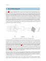


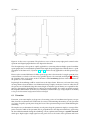


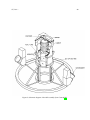


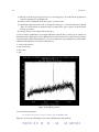
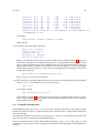
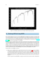
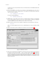
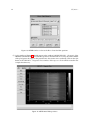
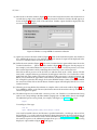
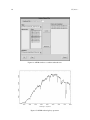


![CURSA [1ex] Catalogue and Table Manipulation](http://vs1.manualzilla.com/store/data/005911996_1-56034bbec42ed74359b0b23f04aae37f-150x150.png)