Download Summations of Waves - Carlson Center for Imaging Science

SIMG-232 LABORATORY #1
Writeup Due 3/23/2004 (T)
1
ONE- and TWO-DIMENSIONAL HARMONIC OSCILLATIONS
1.1
Rationale:
This laboratory (really a virtual lab based on computer software) introduces the concepts of harmonic
oscillations and the effects that result when multiple harmonic oscillations are superposed (added) in
one and two dimensions. The 1-D case illustrates concepts that are relevant to temporal and spatial
coherence, diffraction, and interference of electromagnetic radiation, though these more advanced
applications will not be considered until later in the course. The 2-D case is a generalization of
the √
description of oscillations using complex notation; z ≡ a + ib, where [a, b] are real numbers and
i ≡ −1.
A “harmonic” oscillation is composed of a single sinusoidal frequency. Projections of 2-D harmonic oscillatory motion onto any radial line through the origin in the 2-D plane yields examples
of 1-D harmonic oscillatory motion which all have the same frequency and amplitude, and with the
initial phase determined by the particular axis chosen.
1.2
Preparation:
1. Write the general equation for a simple harmonic oscillation in trigonometric form (i.e., as a
function of the trigonometric functions sine, cosine, etc.).
2. Draw a diagram of the motion of a harmonic oscillator as a function of time, including a graph
of the output as a function of time. Designate on the drawings the amplitude, period, angular
frequency, phase angle, and initial phase, and specify the units for each.
1.3
Procedure:
The lab utilizes two (ancient, but still serviceable) DOS programs: WAVE.EXE and SIGNALS.EXE.
The first was written by Taek Gyu Kim, a former graduate student in Imaging Science, and allows
both 1-D and 2-D sinusoids to be added and displayed dynamically. I wrote the second program to
demonstrate signal processing operations, though it allows sums and products of various signals to
be computed and displayed in various graphical formats. Note that if you run these programs in
the WINDOWS environment, the graphics screens can be captured to the clipboard and pasted into
WINDOWS application programs (such as WORDT M or POWERPOINTT M ). This capability is
useful when doing lab writeups. The image of a graphics screen may be captured to the WINDOWS
Clipboard by pressing simultaneously the “ALT” and “PRINT SCREEN” keys. Once captured, the
graphics screen may be copied into a WINDOWS application by pressing the “CTRL” and “V”
keys simultaneously when running the desired application. You can toggle between the “full-screen
graphics” mode for the DOS programs and the normal WINDOWS screen by simultaneously pressing
“ALT” and “ENTER”. The full WINDOWS screen may be captured to the Clipboard by pressing
just the “PRINT SCREEN” key.
1.3.1
Summation of 1-D oscillations using WAVE.EXE
The summation of same-frequency and different-frequency oscillations will be investigated. To run
the program:
1. Start the program by double-clicking on the WAVE icon or by double-clicking on the filename
WAVE.EXE, which is located in the SIMG-232 directory.
2. Select the plotting speed (1=slowest,10=fastest); try 5 to start.
1
3. Select option 2 for linear superposition, where the oscillations are added in one direction;
4. Select the amplitude A (0 ≤ A ≤ 1), angular frequency ω (listed as “w” on the computer),
which is measured in units of 2π radians per unit time, and initial phase angle φ (in units of
π
2 radians) for both waves;
5. Sit back and watch the action. The “ESCAPE” key stops the motion and asks whether you
wish to continue. Typing n aborts the program, while typing y returns you to the choice of
type of oscillations to add. Note that you cannot restart the oscillation you were running after
typing “ESCAPE” .
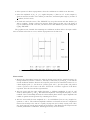
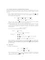
The graphics screen obtained after summing two oscillations is shown below: the input oscillations are shown in the first two rows, and the superposition in the third row.
Screen shot of the 1-D waves display (shown as “negative” to lighten the image).
Observations:
1. Measure the relationship between the selected plotting speed and the angular frequency by
timing oscillation cycles for a selected ω; this may be done easily by setting A2 = 0 so that the
second oscillation vanishes. Measure the temporal period for several numerical values of ω at
a fixed display speed (i.e., the choice of “plotting speed scale”), plot the results, and perform
a linear regression to fit a line to the data. Record the correlation coefficient of the linear
regression. Plot the data and the regression line.
2. Add two waves with the same angular frequency ω, different amplitudes A1 and A2 , and
arbitrary initial phases φ1 and φ2 . Determine the amplitude A and angular frequency ω of the
resultant. Find a relationship between the relative initial phase and the output amplitude and
confirm it against motions generated by summing other waves.
3. Add two waves with the same amplitude A1 = A2 and different (but not very) angular frequencies ω 1 and ω 2 . The resultant amplitude oscillates as a function of time in a complicated
motion that actually is the sum of a rapidly varying term and a slowly varying term. Measure both temporal periods and compute the frequencies. This illustrates the important and
common phenomenon of “BEATS”, which appear in may areas of science.
2
1.3.2
Summation of 1-D oscillations using SIGNALS.EXE
The software SIGNALS.EXE was written to illustrate concepts of linear systems and Fourier transforms, but it also is useful to demonstrate properties of complex numbers and functions, optics, and
digital image processing. The program may be downloaded for free from the CIS website at:
http://www.cis.rit.edu/resources/software/
An online User’s Manual is available at
http://www.cis.rit.edu/resources/software/sig_manual/index.html
A “WINDOWS” version of the program will be available soon.
Many different functions may be entered into the program from the FUNCTIONS menu (option
“F”). The functions are entered as sampled arrays of selectable size (N = 2m for m = 1, 2, . . . , 13, so
that n = 2, 4, 8, . . . , 8192. There are two arrays available: f1 [n] and f2 [n], operate on single functions
from the OPERATIONS menu (option “O”), combine two functions from the “ARITHMETIC”
menu (option “A”), and graph them from the “PLOT” menu (option “P”).
To run the program:
1. Start the program by double-clicking on the SIGNALS icon or by double-clicking on the filename SIGNALS.EXE, which is located in the SIMG-232 directory.
2. Load a function from the FUNCTIONS menu (obtained by typing “F” from any menu). All
functions are loaded in a specific sequence:
f [n] = Re {f [n]} · mR [n] + Im {f [n]} · mI [n]
(a)
(b)
(c)
(d)
Real Part of the function f [n], Re {f [n]}
Modulation of the real part of the function mR [n]
Imaginary Part of the function Im {f [n]}
Modulation of the imaginary part mI [n]
Multiple functions may be added at each step, i.e., you can enter a sinusoidal function
and a rectangle function into the real part of the function to produce the sum of the
two. In this section, you will just be entering the real part of a sinusoidal function,
which is option “‘S” in the functions menu. The options for the sinusoid are the period
(measured in samples), the initial phase (measured in degrees, for ease of entering the
data), and the amplitude. The tasks in this section differ from those in the last using
WAVE.EXE because the functions are “spatial” rather than “temporal”, but the concepts
and mathematical results are exactly analogous.
√
3. Enter a sinusoidal function with some period (the default period of N should work fine) into
the first array, initial phase of 0, and unit amplitude. Plot the graph from the “PLOT” menu
(option “P”)
4. Enter a sinusoidal function with the same period, different initial phase, and the same amplitudle into the other array. Graph the function.
5. Graph the sum of the two functions — this may be done by selecting option “+” from the plot
menu, which graphs the sum without changing the numerical values in the arrays. You also
may add the two arrays together in the “ARITHMETIC” menu (option “A”), but this deletes
the original arrays.
6. Graph the sum of two sinusoidal functions with the same amplitudes
but different (though
√
approximately equal) periods, e.g., if N = 256 (default), so that N = 16, try periods of 14
and 18 samples. Explain the result. The expression for what you have evaluated is:
g [x] = cos [2πξ 0 x] + cos [2πξ 1 x] where ξ 0 6= ξ 1
which may be rewritten by applying some trigonometric identities.
3
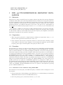
1.3.3
Summation of Perpendicular Oscillations in a Plane Using WAVE.EXE
The summation of two orthogonal oscillations results in a Lissajous figure, which also is called
an Argand diagram when imaginary numbers are plotted on the vertical axis. The two selected
oscillations generate the resulting motion, but the system can considered in the other direction
where the projections of the resulting motion along the x- and y-axis are the selected oscillations.
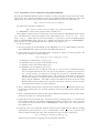
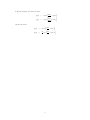
The graphics screen shown below resulted from summation of two oscillations with the same
angular frequency ω and amplitude A, but whose initial phases differed by ± π2 radians.
“Screen shot” of the 2-D waves program
Observations:
1. Add pairs of oscillations to produce: linear vibration along the diagonal, clockwise and counterclockwise circular motion, and elliptical motion where the major axis lies along one of the
Cartesian axes (x or y), and an ellipse whose major axis is at another angle. Also, you are
invited to experiment with the parameters to generate other kinds of figures.
2. If the two oscillations have the same frequency, but arbitrary amplitude and initial phase, what
can you say about the result?
1.3.4
Perpendicular Summation of Arbitrary Functions using SIGNALS.EXE
Procedure:
1. First, replicate one of the cases already considered in Part B by entering a COSINE wave
in the real part with a long period (say 128 samples in an array of size N = 256) and with
initial phase φ0 = 0◦ , and a SINE wave of the same period in the imaginary part (initial phase
φ0 = −90◦ ).
2. Display the function in the PLOT Menu as real-imaginary parts (option “R”), as magnitudephase (option “Q” followed by “U”), and as an ARGAND diagram (option “N”, with other
choices to connect the points, draw symbols at the pixels, and use the SLOW display to allow
the process to be viewed).
4
3. Reenter the arrays but change the initial phase of the imaginary part to φ0 = +90◦ . What is
the difference in the displayed Argand diagram? We speak of the rate of change of the phase
angle of the display as the frequency of the complex function. In this example, the rate of
change of phase is constant, so the frequency is fixed.
4. Reenter the arrays but change the initial phase of the imaginary part to φ0 = +45◦ . What is
the difference in the displayed Argand diagram?
5. One at a time, enter new functions in the REAL and IMAGINARY parts and plot the waves:
(a) REAL Part: SINUSOID (option “S” in the “FUNCTIONS” menu) with period = 64,
amplitude = 1, center pixel = 0, initial phase = 0◦ , IMAGINARY Part: SINUSOID with
period = 64, amplitude = 12 , center pixel = 0, and initial phase = −90◦ .
(b) REAL Part: SINUSOID (option “S” in the “FUNCTIONS” menu) with period = 64,
amplitude = 1, center pixel = 0, initial phase = 0◦ , IMAGINARY Part: SINUSOID with
period = 48, amplitude = 1, center pixel = 0, and initial phase = −90◦ .
(c) REAL Part: SINUSOID (option “S” in the “FUNCTIONS” menu) with period = 64,
amplitude = 1, center pixel = 0, initial phase = 0◦ , IMAGINARY Part: SINUSOID with
period = 64, amplitude = 1, center pixel = 0, and initial phase = −45◦ .
(d) REAL Part: SINUSOID (option “S” in the “FUNCTIONS” menu) with period = 64,
amplitude = 1, center pixel = 0, initial phase = 0◦ , IMAGINARY Part: SINUSOID with
period = 64, amplitude = 1, center pixel = 0, and initial phase = −135◦ .
(e) REAL Part: CHIRP function (option “C” in the “FUNCTIONS” menu) with period =
64, amplitude = 1, center pixel = 0, and initial phase = 0◦ , IMAGINARY Part: CHIRP
with period = 64, amplitude = 1, center pixel = 0, and initial phase = −90◦ . What is
different about the “frequency” of this function compared to that where the REAL and
IMAGINARY parts are sinusoidal functions?
6. In all cases, view the results as real-imaginary parts (option “R” in the “PLOT” menu), as
magnitude/phase (option “M” or option “U” followed by “Q” in the “PLOT” menu) and ,
and as the ARGAND diagram (option “N” in the “PLOT” menu).
7. Repeat the procedure for a few other functions (your choice). For example, enter sinusoids of
equal amplitudes and a phase difference of ±90◦ , and modulate the function by multiplying
the entire function by a decaying function such as a negative exponential. View the Argand
diagram (option “N” in the “PLOT” menu).
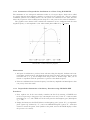
“Screen shot” of Argand diagram in “SIGNALS.EXE”
5
1.3.5
Nonlinear Operations on Sinusoidal Waves in Signals
In all of the steps thus far, the output has been the a single wave or the summation of two or more
sinusoidal waves. In this section, we briefly consider the result of a specific “nonlinear” operation
on a wave.
h
i
1. Enter a “bipolar” sinuoidal function into one of the arrays, e.g., f [n] = cos 2π Xx0 . This
function oscillates between amplitudes of ±1 and its average amplitude is 0. This function
may be written in the complex form:
¶¸
¶¸
∙ µ
∙
µ
1
1
x
x
f [n] =
+ exp −i · 2π
exp i · 2π
2
X0
2
X0
1
1
=
exp [i · (2π (+ξ 0 ) x)] + exp [i · (2π (−ξ 0 ) x)]
2
2
√
−1
where ξ 0 ≡ (X0 )
and i ≡ −1. We say that this sinusoid is the sum of two complex
sinusoids: one with spatial frequency +ξ 0 and one with frequency −ξ 0 .
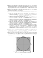
2. Now plot the square of f [n]. You can do this by evaluating the square of the array via option
“^” in the Operations Menu (option “O” from any other menu). After selecting “^”, you then
specify the power to be applied to the amplitude at each poin. The mathematical expression
for this function is:
(f [n])2 = (cos [2πξ 0 x])2
but we can rewrite this using the well-known identity::
(cos [θ])2
=
1
(1 + cos [2θ])
2
2
=⇒ (cos [2πξ 0 x]) =
(cos [2πξ 0 x])
2
=
=
=
1
(1 + cos [2 · 2πξ 0 x])
2
1 1
+ cos [2π (2 · ξ 0 ) x]
2 2µ
¶
1
1 1 1
+
exp [i · (2π (+2ξ 0 ) x)] + exp [i · (2π (−2ξ 0 ) x)]
2 2 2
2
1
1 1
+ exp [i · (2π (+2ξ 0 ) x)] + exp [i · (2π (−2ξ 0 ) x)]
2 4
4
This is composed of a cosine with infinite period and amplitude 12 and two complex-valued
sinusoids that oscillate with frequencies ±2 · ξ 0 with amplitude 14 . In words, the nonlinear
operation has “created” some different spatial frequencies. This did not happen if signals were
just added together.
1.4
Questions:
1. Consider two travelling waves:
¸
2πx
− 2πν 1 t
λ1
∙
¸
2πx
π
y2 (t) = A1 sin
+ 2πν 1 t +
λ1
3
y1 (t) = A1 cos
∙
Find an expression for the sum of the two waves and sketch it as a function of x in the interval
−3λ1 ≤ x ≤ 3λ1 for times t = 0, 2ν11 , ν11 , and ν51 . Label the zero crossings, i.e., the coordinates
x where the wave has zero amplitude.
6
2. Repeat question 1 for the two waves:
¸
2πx
− 2πν 1 t
λ1
∙
¸
2πx
y4 (t) = A1 cos
+ 2πν 1 t
λ1
y3 (t) = A1 cos
∙
and for the waves
¸
2πx
− 2πν 1 t
λ1
¸
∙
A1
2πx
+ 2πν 1 t
cos
2
λ1
y5 (t) = A1 cos
y6 (t) =
7
∙