1
VorDyn1.0 user manual
Stefano Boccelli
February 2014
1
Fast presentation..
Hello, everyone! My name is Stefano Boccelli and I’m a student of
Aerospace (actually, Aeronautic) Engineering at Politecnico di Milano,
Italy. After the last exam session, waiting for new lessons to start, I’ve
written this Vortex Lattice code for MATLAB as a spare time project.
This software is surely buggy and odd written, but I tried to make
it as simple as possible, and also to deeply comment strange lines of
code. You can calculate aerodynamic forces and stability derivatives
with VorDyn, and more..
There’s plenty of software that does the same my softer does, and
does it better.. Tornado for example is one of them. AVL is another!
There are also commercial codes etcetera. The goal of my script is
supposed to be providing a fast access to geometry modification in a
hands-on-code style. What else... as I told you the code is probably
full of bugs or mathematical mistakes, so don’t get angry with me if
the numerical results cause you to be fired or to retrieve a bad mark
at school! :)
Hope you enjoy!
- Stefano -
2
Contents
1 Introduction to the software
4
2 Functionalities
5
3 Geometry Construction
3.1 Aileron or Flap? . . . .
3.2 Winglets . . . . . . . .
3.3 Horizontal Tail . . . .
3.4 Vertical Tail . . . . . .
.
.
.
.
.
.
.
.
.
.
.
.
.
.
.
.
.
.
.
.
.
.
.
.
.
.
.
.
.
.
.
.
.
.
.
.
.
.
.
.
.
.
.
.
.
.
.
.
.
.
.
.
.
.
.
.
.
.
.
.
.
.
.
.
.
.
.
.
.
.
.
.
.
.
.
.
.
.
.
.
.
.
.
.
.
.
.
.
8
9
9
9
9
4 Performing an Analysis
10
5 Program Structure
11
6 Vortex-Lattice Method
12
7 Stability Derivatives
7.1 Angle Derivatives . . . . . . . . .
7.2 Roll, Pitch, Yaw Rate Derivatives
7.3 α̇ Derivatives . . . . . . . . . . .
7.4 Adimensionalization . . . . . . .
7.5 Adjustments . . . . . . . . . . . .
14
14
14
14
14
14
.
.
.
.
.
.
.
.
.
.
.
.
.
.
.
.
.
.
.
.
.
.
.
.
.
.
.
.
.
.
.
.
.
.
.
.
.
.
.
.
.
.
.
.
.
.
.
.
.
.
.
.
.
.
.
.
.
.
.
.
.
.
.
.
.
.
.
.
.
.
.
.
.
.
.
.
.
.
.
.
8 Flight Dynamics modes
15
9 Validation
16
10 Thanks to..
18
3
1
Introduction to the software
Vordyn is basically a vortex-lattice method (actually, a vortex ring method)
that can evaluate aerodynamic properties of a given aircraft geometry. The
reference conditions are stored in the Initial Conditions.m file.
Why the name ”VorDyn”?? Because my idea was originally to implement
a vortex lattice method to obtain stability derivatives and solve the aircraft
dynamical system. Then, since it always takes longer than you expected, I
ran out of time and havn’t tested the dynamical part very much.
This is a Vortex Lattice method, which gives a solution of the potential
flow, that’s why the initial (linearization) condition must be in the linear
aerodynamics field: the method won’t take stall or any kind of flow separation
into account.
A Prandtl-Glauert correction is still not implemented: LOW SUBSONIC
CODE. If you like, you can do it by hand! :)
The code can return some different outputs (see ”functionalities” paragraph), mainly:
• aerodynamic forces
• control surfaces deflection
• stability derivatives
• mesh exporting
• longitudinal and lateral modes
• etc..
Which geometries can I create/process?
You can study airplane geometries composed by one wing, one horizontal tail
and one or two vertical tails. Clearly, tails can be canard surfaces if you like:
you just have to put them in the right place.
Every Lifting surface can be composed by more segments, each one with
control surfaces or flaps.
What if you don’t want the tail? Just put the tail somewhere far from
your wings and set them to be very very very very small! Numerical and
model errors will do the rest.
Fuselage not implemented yet.
4
2
Functionalities
To tell the program what to do, you set 1 or 0 flags in the What To Do.m
file. See the ”Performing an Analisys” Paragraph. Let’s now see what the
code can do, by analizing the variables in the What To Do file. Open it and
you will find the following:
1. Geometry Various
• surfaces and aerodynamic chords: the surface of every wing,
horizontal tail and vertical tail section is calculated and printed on
a file. Mean aerodynamic chords of wing and tail are calculated
too. The file is called ”Surfaces and Chords.dat”.
• plot normal vectors: geometry and panel normal vectors are
plotted.
2. Aerodynamic Forces
• plot cp vectors plots geometry and the Pressure Coefficient acting on every panel.
• total aerodynamic forces writes on the file ”Calculated Total
Aerodynamic Forces.dat” the aerodynamic forces Lift, Drag, Sideforce, Fx, Fy, Fz, Mx, My, Mz generated by the whole configuration.
• component aerodynamic forces: the same, but separating the
wing, horztail and verttail contribute. Filename: ”Calculated
Component Aerodynamic Forces.dat”.
• panel aerodynamic forces writes on a file the forces Fx, Fy, Fz
generated by every single panel, and also the relative Coefficient
of Pressure CP . The panels coordinates are printed too.
3. Component Aerodynamics
• neutral point computation calculates the position of the neutral point by evaluating the pitching moment in two different reference points.
5
• aerodynamic centers lifting derivatives computes the aerodynamic center of wing and horizontal tail and the derivatives
Lα and Mα of stand alone wing and tail. The position of aerodynamic centers is plotted and printed on a file called ”Aerodynamic Centers.dat”, while wing and tail α-derivatives are available
as internal variables.
4. Stability Derivatives
• longitudinal derivatives: longitudinal stability derivatives are
evaluated around the linearization condition set in the Initial
Conditions file. The output is written to a file called ”Stability Derivatives Longitudinal.dat”.
• lateral derivatives the same as for lateral derivatives.
5. Longitudinal Modes
A dynamical system (simplified to take only longitudinal variations
into account) is created and solved. Inertial properties are stored in
the Various Properties.m file. Be careful, because I haven’t tested this
module much..
• eigenvalue plot longitudinal plots the 4 eigenvalues of the longitudinal plane.
• eigenvectors plot longitudinal plots two of the longitudinal
plane eigenvectors on an Argand diagram.
• state matrix export longitudinal: you may be interested in
the state matrix, for various purposes, like studying an automatic
control system for example. The matrix is written on a file named
”Longitudinal State Matrix.dat”.
6. Lateral Modes
the same as Longitudinal Modes:
• eigenvalue plot lateral
• eigenvectors plot lateral
• state matrix export lateral: file ”Lateral State Matrix.dat”.
6
7. Mesh Esporting
you may find useful to create a vortex mesh with VorDyn.. who knows..
you can export it: a file called ”Generated Mesh.dat” is created and
it contains the position of control points (where tangency condition is
imposed), the components of normal vectors for every control point,
the area of every panel and the position of the vertices of the vortex
on a certain panel. Note that the area of the panels is the area of
the surface surrounded by the vortex, for every panel except for those
placed at the trailing edge! Since trailing edge rings go to infinity, the
area of the lifting surface panel must be calculated in a different and
fictitious way.
Every upper-case variable causes a call to a certain MODULE, called MODULE UpperCaseVariableName. The MODULE checks the lower case variables and if they are set to 1 executes the operations.
7
3
Geometry Construction
You can create the geometry by editing the file ”Geometry.m”. Let’s now
focus on tge wing (the rest is the same). The wing can be composed by
many segments, with different sweep angle, dihedral, root inclination, trailing
edge flaps/ailerons or not, different number of mesh vortices in the spanwise
direction, and variable pitch along the wing. An example of wing geometry
may look like this:
Nc wing is the number of panels chordwise. It is the same for every wing
section.
xA wing, yA wing, zA wing are the coordinates of the leading edge of the
root section.
SYM: if you set this flag to one, the wing will be complete, otherwise,
you will have only the right wing.
After setting those parameters, you create the geometry: the length of
the following vectors is the number of the wing sections you create. Each
element is a wing section: if you want your wing to have 57 (hope you don’t)
segments and the 56th to have an aileron, you add 57 elements in the following
vectors and put FCR zero to any of them, and the right flap chord ratio on
the 56th element of the vector!
If you look at the vectors one upon the other, each column of the matrix
you created represents a wing segment.
8
3.1
Aileron or Flap?
Once you have set the FCR of a segment, you choose the deflection angle,
by placing in the vector its value in RADIANS. Note that in the default
”Geometry.m” file, the value between the brackets is in DEG dimensions,
but is converted to radians by multiplying to pi/180.
If you flagged ”SYM = 1”, then the symmetric wing segment will be
created. To tell the software that your surface is an aileron for example, you
set the ”inversion” flag to 1: the deflection of the symmetric flap will be
inverted. You can do that by simply compiling the ”inversion” vector.
3.2
Winglets
If you want to create a vertical surface, you make a segment with a 90o dihedral. Please note that wing geometry is created using an approsite function,
different from the one used for the vertical tail: if you have a wing section
with a huge dihedral (say >45o ), you can’t put flaps on that wing section.
Well, you could, but deflection won’t be the expected because of geometry
creation and rotation issues. Also, the generated vertical surface can’t be
rotated to have an inclination, for the explained reasons.
3.3
Horizontal Tail
The same: horizontal tail too is created using the function wing geometry
function004.
3.4
Vertical Tail
The same philosophy behind wing creation stands for vertical tail too, except
a couple of things:
• SYM flag creates a tail which is symmetrical on the longitudinal aircraft
plane (F18-like twin-tail configuration!)
• lambdavect is still the sweep and deltavect the dihedral: a 0 value means
”vertical tail really vertical”, perpendicular to the xy plane.
The Geometry.m file is an input for other scripts like Geometry Creator.m...
but just let it do the job for you.
9
4
Performing an Analysis
1. Create the Geometry by editing the default Geometry.m file, or if
you already have, call your Geometry file ”Geometry.m” and replace
the original.
2. Set inertial properties in the Various Properties.m file.
3. Tell the program what to do: set the flags in the What To Do.m
file. Do you want to perform some aerodynamic force analysis? Then
set the upper case variable ON (1). Now.. which one of the available
analysis do you want to perform? Set the lower case variable. You can
perform more simulations at once!
4. Oh, I forgot, set the initial conditions! Edit the Initial Conditions.m
file. Set Vinf , rho, alpha0 and beta0. beta0 is the sideslip angle: positive
when the aircraft velocity has a component in the positive Y-body
direction.
5. Run VorDyn.m!!! And possibly yell ”Go-Go-Gadget, VorDyn!”
10
5
Program Structure
Everything starts from VorDyn, which imports the geometry (Geometry.m
file) and the flight conditions (Initial Conditions.m file), then the geometry is
created: Geoemtry Creator calls some functions (wing geometry function004)
for every single lifting segment of the wing and tails, collecting data and
building big vectors and matrices. These are the infos needed for plotting,
mesh exporting or further processing. Then a sequence of if statements starts,
checking the flags set in the What To Do.m file. When a flag is found to be
1, a MODULE is called. I call MODULE a script that collects the operation
of the same type. For example, the MODULE Aerodynamic Forces contains
the following operations:
• print on a file the total forces
• print on a file the forces generated by every aircraft component
• print forces generated by every single panel
How do I activate those sub-tasks? By setting the relative ”sub-flag” in the
What To Do file! In the MODULEs you can find some more if statements
to check that.
11
6
Vortex-Lattice Method
First of all, I strongly suggest the book Low Speed Aerodynamics, by Joseph
Katz and Allen Plotkin. It’s basically a text about numerical panel methods for solving the incompressible flow, and.. it’s a kind of holy textbook for
aerodynamics students!
Ok, let’s talk about VorDyn. As you can see, the created geometry is not
thick at all: as a matter of fact, the code is a ”lifting surface method”.
The implemented method consists in some steps:
1. Preparing the geometry
i dividing the surface into panels
ii finding the quarter-chord line and the 3/4 line of every panel
iii placing a vortex ring (of unknown intensity Γi on the panels: starting from the quarter-chord line of a panel and ending to the quarter
chord of the next panel in chordwise direction. The vortex of the
trailing edge panels is a horseshow vortex (a ring vortex with an
arm placed at infinity), running in the direction of the stream. I
set this ”lone arm” at 300 chords away.
iv locating control points, one for each panel, placed in the middle of
the 3/4 chord line. As a result, the control point will be situated
in the middle of the vortex ring.
v creating normal vectors and surfaces. Unfortunately, a quadrilateral (one of our panels) is not necessarily a planar surface: ”finding”
the normal vector of a skew quadrilateral is mostly a question of
”inventing” the normal vectors. Several methods are available; I use
the cross product of the quadrilateral diagonals. This also allows
me to compute an approximated panel surface.
The points i to v are implemented in the functions wing geometry function004()
and vtail geometry function004().
The vectors xcv, ycv, zcv are filled with coordinates of the control
points in global axis.
xnv, ynv, znv are the ”xyz normals vector”: components of the normal
vectors in the x, y, and z direction. Clearly numel(xnv) == numel(xcv).
12
Vortices are stored in the xvortic,yvortic,zvortic matrices: the size of
them is 4 x numel(xcv). Every column is a vortex ring: the four rows
are the coordinates of every vortex corner.
IMPORTANT: the vortex must be percurred in a certain direction (always the same for every section of every lifting surface of any wing/tail),
or the result will be a complete mess..
2. Induced Velocity Calculation
For every control point, the velocity induced by the vortices is calculated using the well known Biot-Savart law. There are mainly two ways
to do that: matricial operation of for cycles. I’ve implemented the second one, which is reeeeeally slower! I implemented also the first, but it
was not working properly and unfortunately my spare time is almost
over.
The induced velocity calculation is performed by the Vortex Lattice
INDUCEDVELOCITYFUNCTION() function. The function internally
imports the geometry and returns the MAT matrix. Only the constant
term is now needed to solve the linear system and find the circulations!
[MAT] {Γ} = - {ff}
3. The Constant Term The constant term is where the main variables
come in: {ff} is basically the dot product of the free stream velocity
and the normal vector of every panel. By modifying the β and α angles,
we can calculate the results in that α, β condition.
We can find the stability derivatives by solving two times the main
linear system: the first time with a certain {ff} and the second one
with a constant term {ff} evaluated with incremented angles.
4. Forces and Moments
From {Γ}, we can easily obtain aerodynamic loads thanks to the KuttaJoukowski theorem! Moments are obtained multiplying the forces for
the distance from the center of mass of the vehicle.
Lift, Drag and Sideforce are calculated as geometrical projection of the
total Force in wind axis.
13
7
7.1
Stability Derivatives
Angle Derivatives
Calculating an estimation of α and β derivatives is pretty easy: the software
performs a couple of force and moment evaluations with 2 different angles;
the stability derivative is simply (Force2 - Force2 )/(angle2 - angle1 ).
Attention: stability derivatives are evaluated in the linearization conditions, so the ”angle” is in reality an increment.
7.2
Roll, Pitch, Yaw Rate Derivatives
The computation of angular rate derivatives is easy too (although requiring
some small adjustment by you if the calculated derivative values are odd or
the flow velocity is much different from the default 50m/s: see ”Adjustments”
paragraph): a triangular velocity profile centered in the CG is added to the
stream velocity.
7.3
α̇ Derivatives
For the α̇ derivatives, my ideas weren’t that fast-implementing, so I decided
t lt
, data that
to exploit an analitic expression, involving CLα tail and v̄ = SSc
VorDyn can easily calculate.
7.4
Adimensionalization
To provide adimensional coefficientsm forces and angular rates are divided
qc
pb
rb
by the following factors: p̂ = 2V
, q̂ = 2V
, r̂ = 2V
, where p, q and r are the
roll, pitch and yaw rate.
7.5
Adjustments
Angular derivatives are easy to be found: you just set an increment of few
degrees (1o in my case) in the MODULE Stability Derivatives, but angular
rate derivatives are a little more touchy.. A nice way to set them would be
starting from the stream velocity, composing a velocity triangle and setting
the angular rate increment so that tan(1◦ ) = qlVt : the angular rate causing
the incidence of the tail to vary of 1◦
14
8
Flight Dynamics modes
The flying aircraft is subject to different aerodynamic forces: as a first approximation, some are almost proportional to an angular position like angle
of attack or sideslip (we can see them as stiffnesses), others to the velocity
and in the end we have inertial terms. As a result, the aircraft is a dynamical
system, subject to well known flight modes.
Phugoid, short period and the ”third mode” are linked to the longitudinal
plane, while the roll mode, the spiral mode and the dutch roll mode are
latero-directional modes.
Knowing the damping ratio and the natural frequency of those modes is
important to ensure proper flight qualities; ensuring the modes are stable (or
not too much unstable) is a fundamental requirement for succesful and safe
flight.
By filling a couple of matrices with proper stability derivatives, VorDyn
accepts the Hypothesis of small perturbations and studies separately the
longitudinal and the latero directional planes, solving two separated linear
systems.
Eigenvalues are plotted on the Gauss plane and Eigenvectors on the Argand Diagram: a plot of the magnitude and the phase of the states involved
in a certain mode.
ATTENTION! The results are clearly strongly affected by the inertial
properties (to be set in the Various Geometry.m file) and by the CG position
(static margin). Also, I’m not that sure of having well compiled matrices and
all, so... you better be careful with my results!!!
15
9
Validation
I shall now compare the results of my code with other data. First of all a naif
and very crude validation have been made, comparing the lift computed on
a finite wing geometry to the theoretical lift generated by a wing immerged
into bidimensional current: L = 12 ρV 2 SCL . CL is 2πα, as stated by the small
perturbances theory. Creating four wings with increasing aspect ratios I verified that the relative error, between numerical Lift and theoretical 2D Lift,
decreased. Of course a real validation would have passed through Prandtl
finite wing model!
The software Tornado is the result of a Magistral Thesis work. In one of
the final chapters of the thesis, stability derivatives of a Cessna 172 Skyhawk
are calculated and compared with experimental data. I add here my results,
calculated (like Tornado) in a reference point located at 31.9% of the wing
mean aerodynamic chord.
16
Derivative
CL
CD
CL α
CD α
Cm α
CY β
Cl β
Cn β
CY p̂
Cl p̂
Cn p̂
CY r̂
Cl r̂
Cn r̂
*
**
Experimental Tornado
0.386
0.386
0.042
0.006
4.41
5.27
0.182
0.17
-0.0409
-1.55
-0.35
-0.47
0.103
0.008
0.0583
0.197
-0.0925
-1.87
-0.483
-0.484
-0.035
-0.846
0.175
0.091
0.1
0.03
0.086
0.038
VorDyn
0.3812
0.0212
5.019
0.2409
-1.358
-0.287
-0.0233*
0.1159
-0.1146
-0.2567
0.0278**
0.2652
0.0129
-0.0269*
convention is clearly different
I’m afraid something’s wrong in my code..
And now a figure of the Skyhawk geometry created. Vortex rings are
displayed in green.
17
10
Thanks to..
Special thanks to Politecnico di Milano that, inter alia, provided some of the
electric current that powered my laptop :)
Thanks to all the scientists and engineers who discovered and built the
aerodynamic knowledge we have today.
18