Download User`s guide

SWarp
v2.15
User’s guide
E. BERTIN
Institut d’Astrophysique & Observatoire de Paris
December 10, 2004
Contents
1 What is SWarp?
1
2 Skeptical Sam’s questions
1
3 Installing the software
2
3.1
Software and hardware requirements . . . . . . . . . . . . . . . . . . . . . . . . .
2
3.2
Obtaining SWarp . . . . . . . . . . . . . . . . . . . . . . . . . . . . . . . . . . .
2
3.3
Installation . . . . . . . . . . . . . . . . . . . . . . . . . . . . . . . . . . . . . . .
2
4 Using SWarp
4.1
3
The Configuration file . . . . . . . . . . . . . . . . . . . . . . . . . . . . . . . . .
3
4.1.1
Creating a configuration file . . . . . . . . . . . . . . . . . . . . . . . . . .
3
4.1.2
Format of the configuration file . . . . . . . . . . . . . . . . . . . . . . . .
3
4.1.3
Configuration parameter list
3
. . . . . . . . . . . . . . . . . . . . . . . . .
5 How SWarp works
7
5.1
Overview of the software . . . . . . . . . . . . . . . . . . . . . . . . . . . . . . . .
7
5.2
Image mapping and memory constraints . . . . . . . . . . . . . . . . . . . . . . .
7
5.3
Propagating FITS keywords . . . . . . . . . . . . . . . . . . . . . . . . . . . . . .
10
5.4
Parallel processing . . . . . . . . . . . . . . . . . . . . . . . . . . . . . . . . . . .
10
5.5
Astrometry . . . . . . . . . . . . . . . . . . . . . . . . . . . . . . . . . . . . . . .
10
5.5.1
Input frames . . . . . . . . . . . . . . . . . . . . . . . . . . . . . . . . . .
10
5.5.2
Output frames . . . . . . . . . . . . . . . . . . . . . . . . . . . . . . . . .
11
5.5.3
Bi-cubic spline interpolation . . . . . . . . . . . . . . . . . . . . . . . . . .
15
Resampling . . . . . . . . . . . . . . . . . . . . . . . . . . . . . . . . . . . . . . .
15
5.6.1
Image data . . . . . . . . . . . . . . . . . . . . . . . . . . . . . . . . . . .
16
5.6.2
Oversampling . . . . . . . . . . . . . . . . . . . . . . . . . . . . . . . . . .
18
5.6.3
Noise stability issues . . . . . . . . . . . . . . . . . . . . . . . . . . . . . .
18
5.6.4
Weight-maps . . . . . . . . . . . . . . . . . . . . . . . . . . . . . . . . . .
21
5.7
Background subtraction . . . . . . . . . . . . . . . . . . . . . . . . . . . . . . . .
21
5.8
Scaling the flux . . . . . . . . . . . . . . . . . . . . . . . . . . . . . . . . . . . . .
24
5.9
Combining resampled images . . . . . . . . . . . . . . . . . . . . . . . . . . . . .
25
5.9.1
Various types of image combination . . . . . . . . . . . . . . . . . . . . .
25
5.9.2
Weighted coaddition . . . . . . . . . . . . . . . . . . . . . . . . . . . . . .
27
5.9.3
Image buffering and memory constraints . . . . . . . . . . . . . . . . . . .
29
5.6
i
6 Two-step co-addition and resampling
29
7 Examples
29
7.1
Example 1 . . . . . . . . . . . . . . . . . . . . . . . . . . . . . . . . . . . . . . . .
30
7.2
Example 2 . . . . . . . . . . . . . . . . . . . . . . . . . . . . . . . . . . . . . . . .
31
8 Troubleshooting
33
9 Acknowledgements
33
ii
iii
1
What is SWarp?
SWarp is a program that resamples and co-adds together FITS images using any arbitrary
astrometric projection defined in the WCS standard1 . The main features of SWarp are:
• FITS format (including multi-extensions) in input and output,
• Full handling of weight-maps in input and output,
• Ability to work with very large images (up to 500 Mpixels on 32-bit machines and 10 6
Tpixels with 64-bits), thanks to customized virtual-memory-mapping and buffering,
• Works with arrays in up to 9 dimensions (including or not two spherical coordinates),
• Selectable high-order interpolation method (up to 8-tap filters) in any dimension,
• Compatible with WCS and TNX (IRAF) astrometric descriptions,
• Support for equatorial, galactic and equatorial coordinate systems,
• Astrometric and photometric parameters are read from FITS headers or external ASCII
files,
• Built-in background subtraction,
• Built-in noise-level measurement for automatic weighting,
• Automatic centering and sizing functions of the output field,
• Multi-threaded code with load-balancing to take advantage of multiple processors.
2
Skeptical Sam’s questions
Skeptical Sam doesn’t have time to test software extensively but is always keen on asking
agressive questions to the author to find out if a program could fit his needs.
S.Sam: What’s the point in releasing another image co-addition software? We already had the
Drizzle and MSCRED (IRAF) packages, for instance.
Author: Co-addition is most-certainly the most critical step in reducing modern CCD mosaic
data. Although several powerful packages are already available, they did not meet all the
requirements we have at the TERAPIX data center here in Paris.
S.Sam: SWarp doesn’t perform the astrometric calibration, does it?
Author: No it doesn’t. The astrometric calibration software of the TERAPIX pipeline will be
released in future versions of the software. In the meanwhile, any polynomial description will
do; you may use IRAF for instance.
S.Sam: I am the kind of guy who does high precision astrometry and photometry. My sources
are detectable on raw frames. Resampling, you know, would just wreck the signal, so I prefer
to combine measurements from individual images than to co-add pixels.
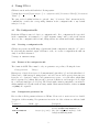
Author: It is true that resampling distorts slightly both signal and noise. However, if done
properly, and if the data are not undersampled (Full Width at Half Maximum > 2.5 pixels),
1
see http://www.cv.nrao.edu/fits/documents/wcs/wcs.html
1
the degradation is generally very small. For instance, resampling a single ground-based image
(atmospheric seeing of FWHM 3 pixels, and conversion factor 2e− /ADU) twice with SWarp,
and comparing fluxes and positions measured using PSF-fitting, one gets for bright stars rms
differences of less than 5.10−4 mag and 10−3 pixel between the original and the twice-resampled
images. This is already much better than what photon-noise allows for. Hence apart from
situations of strongly non-stationary noise or undersampled data, the consequences of resampling
are expected to be negligible.
3
3.1
Installing the software
Software and hardware requirements
SWarp has been developed on Unix machines (Compaq Tru-64 and GNU/Linux), and should
compile on any POSIX-compliant system. The software is run in (ANSI) text-mode from a shell.
A window system is therefore unnecessary with present versions.
Memory requirements are fairly modest in most cases, as they do not depend on the size of
the output images. 100MB is sufficient when co-adding images (even mosaics) involving current
CCD chips (2k×4.5k). More memory may be helpful for co-adding bigger maps. Although the
built-in virtual-memory feature will almost always allow one to work with any image size, the
performance hit caused by file-swapping may be important in some cases.
3.2
Obtaining SWarp
The easiest way to obtain SWarp is to download it from an internet site. The current official
anonymous FTP site is ftp://ftp.iap.fr/pub/from users/bertin/swarp/. There can be
found the latest versions of the program as standard .tar.gz Unix source archives, including
the documentation, and Linux binaries as RPM packages. For production, it is strongly advised
to install the RPM packages if you are running Linux on a machine with ix86 architecture
and RPM-support, as they contain a strongly optimized version of the code. The “-MP” (multiprocessor) version can take advantage of multiple processors in an SMP (or even hyperthreaded)
configuration by running several threads at the same time.
3.3
Installation
To install, you must first uncompress and unarchive the archive:
gzip -dc swarp-x.x.tar.gz | tar xvf A new directory called swarp-x.x should now appear at the current position on your disk. You
should then just enter the directory and follow the instructions in the file called “INSTALL”.
The software is also available as a precompiled RPM for Linux systems with an x86 architecture.
The multithreaded version (with the mp suffix in the filename) shall be installed preferably on
machines with multiple processors, to take advantage of parallel processing. The simplest way
to install an RPM package is to log as root and use the following command
rpm -U swarp-x.x-dist.arch.rpm
2
4
Using SWarp
SWarp is run from the shell with the following syntax:
% swarp Input image1 [Input image2 ...] -c configuration-file [-Parameter1 Value1] [-Parameter2
Value2 ...]
The part enclosed within brackets is optional. Any ”-Parameter Value” statement in the
command-line overrides the corresponding definition in the configuration-file or any default
value (see below).
4.1
The Configuration file
Each time SWarp is run, it looks for a configuration file. If no configuration file is specified
in the command-line, it is assumed to be called “default.swarp” and to reside in the current
directory. If no configuration file is found, SWarp will use its own internal default configuration.
4.1.1
Creating a configuration file
SWarp can generate an ASCII dump of its internal default configuration, using the “-d” option.
By redirecting the standard output of SWarp to a file, one creates a configuration file that can
easily be modified afterward:
% swarp -d >default.swarp
4.1.2
Format of the configuration file
The format is ASCII. There must be only one parameter set per line, following the form:
Config-parameter
Value(s)
Extra spaces or linefeeds are ignored. Comments must begin with a “#” and end with a linefeed.
Values can be of different types: strings (can be enclosed between double quotes), floats, integers,
keywords or boolean (Y/y or N/n). Some parameters accept zero or several values, which must
then be separated by commas. Integers can be given as decimals, in octal form (preceded by digit
O), or in hexadecimal (preceded by 0x). The hexadecimal format is particularly convenient for
writing multiplexed bit values such as binary masks. Environment variables, written as $HOME
or ${HOME} are expanded.
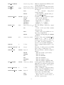
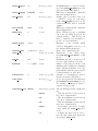
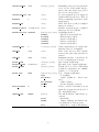
4.1.3
Configuration parameter list
Here is a list of all the parameters known to SWarp. Please refer to next section for a detailed
description of their meaning. New parameters in version 2.0 of the software are indicated with
a “ * ”.
Parameter
default type
Description
BACK DEFAULT
0.0
floats (n ≤ nima )
Default background value to be subtracted in BACK TYPE MANUAL mode.
integers (n ≤ nima ) Size (in background meshes) of the
BACK FILTERSIZE —
background-filtering mask.
3
BACK FILTTHRESH
—
integers (n ≤ nima )
BACK SIZE
BACK TYPE
—
AUTO
integers (n ≤ nima )
keywords (n ≤ nima )
AUTO
MANUAL
CELESTIAL TYPE
NATIVE
CENTER TYPE
ALL
keyword
NATIVE
PIXEL
EQUATORIAL
GALACTIC
ECLIPTIC
keywords (n ≤ ndim )
ALL
MOST
MANUAL
CENTER
0.0
strings (n ≤ ndim )
COMBINE
Y
boolean
COMBINE BUFSIZE*
64
integer
COMBINE TYPE
MEDIAN
keyword
MEDIAN
AVERAGE
MIN
MAX
WEIGHTED
CHI2
strings (n ≤ 1024)
COPY KEYWORDS
OBJECT
DELETE TMPFILES
Y
boolean
FSCALASTRO TYPE
FIXED
keyword
NONE
FIXED
4
Difference threshold (in ADUs) for the
background-filtering.
Size (in pixels) of a background mesh.
What background is subtracted from
the images:
–
the
internal
interpolated
background-map,
– a user-supplied constant value provided in BACK DEFAULT.
Celestial coordinate system in output:
– Same as first input file,
– No (de-)projection (faster),
– Equatorial α, δ coordinates,
– Galactic l, b coordinates
– Ecliptic λ, β coordinates
The way SWarp centers the output
frame:
– Center on the region that contains
all input fields,
– Center on the region with most overlap between input fields,
– Manual centering using the CENTER
parameter.
Position of the center in CENTER TYPE
MANUAL mode.
Can be given in
floating point notation, in hh:mm:ss
(for right ascension/longitude), or
dd:mm:ss (for declination/latitude).
If true, resampled images will be combined.
Amount of buffer memory (in MB)
used for the co-addition process.
The way SWarp combines resampled
images:
– Take the median of pixel values,
– Take the average,
– Take the minimum,
– Take the maximum,
– Take the weighted average.
– Take the weighted, quadratic sum.
Coma-separated list of FITS keywords
that will be propagated from the input
FITS headers to the coadded and resampled image headers.
If true, resampled, temporary image
files are deleted if COMBINE is set to Y.
The way SWarp computes the astrometric part of the flux-scaling:
– Ignore the effects of re-projection,
– Apply a fixed correction based on
the ratio of pixel scales.
FSCALE DEFAULT
1.0
floats (n ≤ nima )
FSCALE KEYWORD
FLXSCALE
string
GAIN DEFAULT
0.0
floats (n ≤ nima )
GAIN KEYWORD
GAIN
string
HEADER ONLY
Y
boolean
HEADER SUFFIX
.head
string
IMAGEOUT NAME
IMAGE SIZE
coadd.fits
—
string
integers (n ≤ ndim )
MEM MAX
128
integer
NTHREADS*
1 or 2 (MP)
integer
OVERSAMPLING
0
integers (n ≤ ndim )
PIXEL SCALE
—
floats (n ≤ ndim )
PIXELSCALE TYPE
MEDIAN
keywords (n ≤ ndim )
MEDIAN
MIN
MAX
MANUAL
FIT
5
Default fluxscale to adopt for each image if the FSCALE KEYWORD keyword is
not found in the FITS header.
FITS keyword that should contain the
flux scale in input images.
Default gain (conversion factor in
e− /ADU) to adopt for each image
if the GAIN KEYWORD keyword is not
found in the FITS header. 0 means
“infinite”.
FITS keyword that should contain the
gain in input images.
If true, SWarp does not do anything
but create the FITS header in the
combined image. This header can
later be duplicated as .head files to
provide on several machines
Extension of the external ASCII
“headers” that shall be seeked to override internal FITS parameters.
Name of the output image file.
Dimensions of the output image
(in PIXELSCALE TYPE MANUAL or FIT
mode).
Maximum amount of megabytes allowed for (silicon) memory storage.
Number of threads (processes) to run
simultaneously during the resampling
phase. SWarp must have been compiled with the threads option enabled
for this parameter to take effect.
Amount of oversampling in each dimension (0 means “automatic”).
Step between pixels in each dimension
(in PIXELSCALE TYPE MANUAL mode).
For angular coordinates, it must be
expressed in arcseconds.
The way SWarp sets the output pixel
size:
– Take the median of pixel scales at
the center of input frames,
– Take the minimum of pixel scales at
the center of input frames,
– Take the maximum of pixel scales at
the center of input frames,
– User-defined pixel scale at image
center (with the PIXEL SCALE keyword),
– Compute the pixel scale in order to
have the full output field fitting the
user-defined IMAGE SIZE.
PROJECTION ERR
0.001
floats (n ≤ nima )
PROJECTION TYPE
TAN
string
RESAMPLE
Y
boolean
RESAMPLE DIR
.
string
RESAMPLE SUFFIX
.resamp.fits
string
RESAMPLING TYPE
LANCZOS3
SUBTRACT BACK
Y
keywords (n ≤ ndim )
NEAREST
BILINEAR
LANCZOS2
LANCZOS3
LANCZOS4
booleans (n ≤ nima )
VMEM DIR
/tmp
string
VMEM MAX
2048
integer
WEIGHT IMAGE
WEIGHTOUT NAME
WEIGHT THRESH
coadd.fits
strings (n ≤ nima )
string
floats (n ≤ nima )
WEIGHT TYPE
NONE
keywords (n ≤ nima )
NONE
MAP WEIGHT
WRITE FILEINFO
N
MAP VARIANCE
MAP RMS
boolean
VERBOSE TYPE
NORMAL
keyword
QUIET
NORMAL
FULL
6
Maximum position error (in pixels) allowed for the bicubic-spline interpolation of the astrometric reprojection.
Use 0 for no interpolation.
Projection system used in output, in
standard WCS notation (see Table 1).
If true, resampling is performed on the
input images.
Path of the directory where resampled
images are written.
filename extension given to resampled
images produced by SWarp.
Resampling method:
– Take the nearest neighbour,
– Bi-linear interpolation,
– Lanczos-2 4-tap filter,
– Lanczos-3 6-tap filter,
– Lanczos-4 8-tap filter.
If true, input images are backgroundsubtracted prior to resampling.
Path of the directory where virtualmemory and other temporary files are
written.
Maximum amount of megabytes allowed for virtual-memory storage.
List of input weight-maps.
File name of the output weight-map.
Threshold below or above which input
weights are equivalent to zero (infinite
variance, i.e. a bad pixel).
Type of input weight-maps:
– no weighting,
– relative weights (i.e. inverse variance),
– relative variance,
– absolute standard deviation.
If true, extended information about
input files is written in the header of
the output FITS image.
How much SWarp comments its operations:
– run silently,
– display warnings and limited info
concerning the work in progress,
– display more complete information.
5
How SWarp works
5.1
Overview of the software
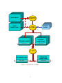
What SWarp does is basically to read a set of input FITS images, resample and combine them,
and finally save the resultant FITS image to disk. The work can be decomposed in several steps:
1. Input image headers are read and checked for content. If configured in fully automatic
mode, SWarp will set the characteristics of the output frame based on this information.
2. Input images (and their weight-maps, if available) are read one-by-one. Background-maps
are built, and subtracted from the images if required.
3. Images are resampled, projected into subsections of the output frame, and saved as FITS
files. “Projected” weight-maps are created too, even if no weight-maps were given in input.
4. A combined output image is created using the information stored in the “projected” weightmaps. It consists of a composite of the resampled sub-sections. A composite output
weight-map is also written in the process.
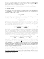
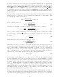
The global layout of SWarp is presented in Fig. 1. Let us now describe each of the important
steps.
5.2
Image mapping and memory constraints
How does SWarp projects input images into the output frame space? There are two ways of
applying a geometric transformation to an image (see Wolberg 1992). The most intuitive is
called “forward mapping”. It consists in scanning the input image pixel-per-pixel, line-by-line.
Each pixel is simply “thrown” to the position it is supposed to occupy in the output grid.
Although this technique can be used for geometric resampling or “drizzling” (Fruchter & Hook
1997), it is totally cumbersome with high order interpolation techniques. “Inverse mapping”
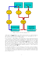
is far more efficient in this case. In this procedure the output frame is scanned pixel-per-pixel
and line-by-line. Using the inverse projection, each output pixel center is associated a position
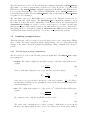
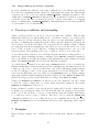
in the input frame, at which the image is interpolated. This technique has been implemented
in SWarp (Fig. 2); it possesses several advantages. The output image is accessed sequentially,
and thus can be arbitrarily large. Also, only positions corresponding to pixels (or sub-pixels)
within the output frame have to be mapped.
The most potentially critical part is the pseudo-random access in the input image. In most cases,
it will be an individual imaging array (like an individual CCD) and will therefore fit in memory.
For much larger input images however we rely on the efficiency of virtual-memory-mapping.
SWarp’s virtual memory engine works in the following way: each input image, stored as a
single precision, 4-byte array is loaded in physical memory if the required amount of megabytes
doesn’t exceed MEM MAX. If it does, a temporary file called vmxxxxx xxxxx.tmp is written in the
directory specified by VMEM DIRECTORY. The program exits with an error message if this file would
exceed VMEM MAX Megabytes. The 3 “memory” parameters are mostly hardware-dependent. It is
advised to set MEM MAX to 50-100% of the actual amount of memory present in your machine. If
disk-space is not the limiting factor, VMEM MAX should be set to a higher value, 2048 on a 32-bit
machine, or even more on a 64-bit machine. The choice of the VMEM DIRECTORY is critical. First,
this write-enabled directory must be large enough to contain each input image in floating-point
format. Second, it is strongly recommended to have the data on a fast disk. Note that the
7
Input frames
Background
subtraction
Input
weight-maps
Image
Resampling
External
headers
Warped images
Warped
weight-maps
Frame buffer
Frame buffer
Co-addition
Co-added image
Composite
weight-map
Frame buffer
Frame buffer
Figure 1: Global Layout of SWarp.
8
Input image
Weight-map
Flux
scaling
Variance
scaling
alpha,delta
->
x,y (in)
x,y (out)
->
alpha,delta
Interpolation
engine
Resampled image
Resampled
weight-map
Frame buffer
Frame buffer
Figure 2: Layout of the image mapping section.
default path for VMEM DIRECTORY is /tmp, which on many systems is on a partition simply not
large enough to handle the typical quantities of data to process. An alternative is to use “.”,
the current directory, at the expense of disk thrashing!
De-projecting and co-adding simultaneously all input images would frequently imply many files
open at the same time, and large amounts of (virtual) memory. SWarp takes a more sequential
approach: each input image is mapped in a tightly-fitting rectangular subsection of the output
frame. All subsections are written to disk (in the RESAMPLE DIRECTORY) as swarp.xxx.fits FITS
files, and read back later during the co-addition phase, to be stacked together. Individual
subsection files are automatically removed after processing or abortion. It is possible to disable
the deletion by setting the DELETE TMPFILES configuration parameter to N (the default is Y).
This can be useful for diagnostic purposes.
Note that although SWarp does not use much memory, the amount of temporary disk-space
needed during processing can be quite large. In addition to the output image and weight-map,
one should provide disk-space for the individual projected images and their weight-maps. In the
case of mappings done at unit scale, this involves storing more than twice the amount of input
pixels as temporary data.
9
5.3
Propagating FITS keywords
During the re-gridding and co-addition processes involved in SWarp, the FITS keywords present
in the input image headers are not automatically copied to the output image headers (many
of them become irrelevant). Nevertheless, for data management purposes it is often useful
to propagate some selected FITS keywords (such as FILTER, EXPTIME or TELESCOP for
instance) and their values from the input image headers to the resampled and coadded image
headers. To this aim, a COPY KEYWORDS configuration parameter is provided. It accepts a list
of FITS keywords that shall be copied in the headers of all the images created by SWarp (by
default, only the OBJECT keyword and its content are copied). But because the coadded image
can result from the combination of many input files, only the keyword found in the first image
header from the input file list is propagated up to the final coadded image. It is important to
note that SWarp does not check the content of the list of COPY KEYWORDS; therefore one should
be cautious not to propagate FITS keywords like NAXIS1,BITPIX,... that may interfere with
the interpretation of the output data.
5.4
Parallel processing
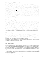
Versions ≥ 1.32 of SWarp can be compiled with “multi-threading” enabled2 . Multi-threading
allows CPU-intensive tasks in SWarp to be run in parallel on Symetric Multi-Processing (SMP)
or Hyper-Threaded (HT) machines. By default, SWarp-MP uses 2 computing threads, which
should lead to a ≈ 1.85× speed-up in resampling compared to the mono-threaded version, on an
SMP machine. The number of computing threads used can be set with the NTHREADS configuration parameter. Best performance is generally achieved with NTHREADS equal to the number of
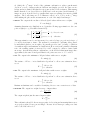
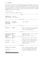
processors in the machine3 . Figure 3 shows the improvement in SWarp pixel throughput as a
function of NTHREADS on a 4-processor machine. Departure from a linear scaling with the number
of threads are mostly due to I/O limitations and parts of code that are not multithreaded.
5.5
Astrometry
The astrometric engine at the heart of SWarp is based on M. Calabretta’s WCSlib library 4 , to
which we added the handling of polynomial distorsion parameters (FITS keywords PV xx xx) as
proposed in the latest WCS documents5 . We included IRAF’s TNX astrometric projection too
(for inputs only), although it is not part of the WCS standard.
All celestial coordinate computations are performed in the equatorial system. Galactic or ecliptic
coordinates are supported in input and output.
5.5.1
Input frames
(De-)projection parameters of input images are extracted from their respective FITS headers.
These are the usual CTYPEx CRVALx, CRPIXx, CDELTx and/or CD xx xx WCS parameters. External “header” files can also be provided by the user; for every input xxxx.fits image, SWarp looks
for a xxxx.head header file, and loads it if present. A .head suffix is the default; it can be changed
2
To check if your SWarp executable is multi-threaded, run it without any argument. Multi-threading is
enabled if the displayed version number is followed by ”-MP”.
3
The actual number of threads started by SWarp is always larger than NTHREADS; but no more than NTHREADS
threads are active simultaneously.
4
Available at http://www.cv.nrao.edu/fits/src/wcs/
5
http://www.cv.nrao.edu/fits/documents/wcs/wcs.html
10
Figure 3: Pixel throughput of SWarp 2.0 resampling (Lanczos3) as a function of the NTHREADS
configuration parameter on an SMP machine with 4 Opteron-242 (1.6GHz) processors. Perfect
linear scaling is indicated by the dashed line for reference.
using the HEADER SUFFIX configuration parameter. External headers may either be real FITS
header cards (no carriage-return), or ASCII files containing lines in FITS-like format, with the
final line starting with “ENDttttt ”. Multiple extensions must be separated by an “ENDttttt ”
line. External “headers” need not contain all the FITS keywords normally required. The keywords present in external headers are only there to override their counterparts in the original
image headers, or add new ones.
5.5.2
Output frames
The celestial pair of components of the output coordinate system is specified with the CELESTIAL TYPE
configuration parameter, and can be selected among NATIVE, PIXEL, EQUATORIAL, GALACTIC and
ECLIPTIC. In NATIVE mode, the output celestial coordinate system is taken from that of the first
file of the input list. This is the default. The PIXEL option forces SWarp to ignore all the “celestial” aspects (projection, de-projection, sky coordinates) of both input and output images. It
provides a major speed-up to the warping engine by bypassing all the trigonometric operations
normally involved in the other modes. It is useful for quickly combining mosaic images whenever
astrometric information is not needed. In PIXEL mode, degrees are interpreted as dimensionless
Cartesian coordinates.
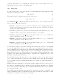
The output (celestial) projection is set by the PROJECTION TYPE configuration parameter. The
list of all presently supported projections is shown in Table 1, and illustrated in Fig. 4 and 5
using a gridded map of the Earth.
Now, what projection is the best? With “small” fields (< 10 degrees in their maximum di-
11
mension), the choice is not critical as long as the projection center lies within the frame. For
compatibility reasons, it is advised to stay with the traditional gnomonic (TAN, for tangential)
projection in such cases. With larger fields the pure tangential projection is inappropriate, and
one is faced with the usual problems confronted by cartographers. It would be outside the
scope of this document to discuss the merits of each projection. For detailed information about
the different projection systems, the user should refer to the latest WCS document. Let us just
mention that equal-area projections (those that conserve relative areas) are often to be preferred
for mapping large sky surveys, because they naturally conserve surface-brightness and/or allow
summing pixel values to measure fluxes. The following are equal-area projections: ZEA, CEA,
COE, BON, GLS, PAR, MOL, AIT, QSC. AIT (Aitoff) is one of the most popular projections for all-sky
maps.
Note that some of the projections (CYP, CEA, COD, COE, COO, COP and BON) require additional
PV xx xx parameters. These parameters can easily be included in a xxxx.head header file with
the same prefix as the output coadded image (which is coadd.fits by default, see the example at
the end of this document).
Centering of the output frame is controlled by the CENTER TYPE parameter. There are three
centering modes:
• ALL: the field is centered in a way that all input images fit into the output frame. This is
the default.
• MOST: the field is centered on the zone of maximum overlap between input images.
• MANUAL: manual centering with the CENTER parameter.
A different centering mode can be used in each dimension; for instance, in 2D images with α, δ
coordinates, “CENTER TYPE ALL,MOST” will apply the ALL mode in α and the MOST mode in δ.
If a single mode is specified, it is applied to all available dimensions.
The CENTER parameters are active in CENTER TYPE MANUAL mode only, and must be used to specify the actual center of the output field, in world units. In the case of angular coordinates, both
the floating point (in degrees) and sexagedecimal formats are accepted: right ascension/longitude
may be written as hh:mm:ss.ss, and declination/latitude as ±dd:mm:ss.ss.
The pixel “scale” (which is the step between pixels at the center of the output frame) can be
computed automatically in each dimension by SWarp. There are five modes specified by the
PIXELSCALE TYPE configuration parameter:
• MEDIAN (the default): the median value of all pixel scales at the center of input frames is
taken as the output pixel scale.
• MIN: the smallest of all pixel scales at the center of input frames is taken.
• MAX: the largest of all pixel scales at the center of input frames is taken.
• MANUAL: manual scaling with the PIXEL SCALE configuration parameter.
• FIT: Pixel scales are automatically computed to have the projected data fitting the output
frame dimensions specified with the IMAGE SIZE configuration parameter.
When right ascension/longitude and declination/latitude are both present, pixel scales computed
by SWarp are made equal in both dimensions to avoid anamorphosis.
12
Table 1: Valid PROJECTION TYPEs in SWarp
Zenithal projections
AZP
TAN
STG
SIN
ARC
ZPN
ZEA
AIR
Zenithal perspective
Distorted tangential
Stereographic
Slant orthographic
Zenithal equidistant
Zenithal polynomial
Zenithal equal-area
Airy
Cylindrical projections
CYP
CEA
CAR
MER
Cylindrical perspective
Cylindrical equal-area
Plate carrée
Mercator
Conic projections
COP
COE
COD
COO
Conic
Conic
Conic
Conic
Pseudoconic and polyconic projections
BON
PCO
Bonne’s equal-area
Polyconic
Pseudocylindrical projections
GLS
PAR
MOL
AIT
Global sinusoidal (Sanson-Flamsteed)
Parabolic
Mollweide
Hammer-Aitoff
Quad-cube projections
TSC
CSC
QSC
Tangential spherical cube
COBE quadrilateralized spherical cube
Quadrilateralized spherical cube
perspective
equal-area
equidistant
orthomorphic
13
AZP
TAN
STG
SIN
ARC/ZPN
ZEA
AIR
CYP
CEA
CAR
MER
COP
COE
COD
COO
BON
PCO
Figure 4: Graphic illustration of projections available in the WCS library (see text).
14
GLS
PAR
MOL
TSC
CSC
QSC
AIT
Figure 5: Graphic illustration of projections available in the WCS library (continued from Fig.
4).
The PIXEL SCALE parameters are active in PIXELSCALE TYPE MANUAL mode only, and must be
used to specify the actual pixel step for each dimension, in world units. Note that in the case
of angular coordinates, PIXEL SCALE values are read in arcseconds, not degrees.
The dimensions of the output frame (in number of pixels per axis) are set using the IMAGE SIZE
configuration parameter. A value of 0 for any axis results in an automatic dimensioning of this
axis; but obviously this is not possible in PIXELSCALE TYPE FIT mode.
Note that the current automatic centering and scaling routines can get confused rather easily
with some very wide field projections. In particular, it is recommended to turn off automatic
settings when making all-sky projections.
5.5.3
Bi-cubic spline interpolation
The trigonometric calculations involved in SWarp re-projections have a major impact on processing speed. To accelerate the resampling phase, versions ≥ 2.06 of SWarp implement a bicubic spline interpolation6 of the astrometric mapping between the input and the output frames.
Interpolation is used by default for large images, with a maximum allowed positional error of
10−3 pixel (as measured in the output frame). This error tolerance can be changed independently
for each input image with the PROJECTION ERR configuration parameter. A PROJECTION ERR of
0 turns interpolation off. Interpolation is also automatically deactivated for smaller images or
inappropriate mappings like all-sky projections or projection with singularities.
5.6
Resampling
The action of projecting a grid of pixels on another grid is called resampling. Ideal image
resampling involves both filtering and interpolation between pixels. In SWarp, filtering is
6
This feature is currently limited to 2D images.
15
“naturally” implemented by oversampling the destination grid. Because SWarp uses reversemapping, interpolation is made on the input images.
5.6.1
Image data
At each position x, the dot-product between a local kernel k(x) and neighbouring pixel values
f yields a local, interpolated value:
f˜(x) = k(x).f
(1)
The kernel is derived locally from an interpolation function h:
ki (x) = h(x − xi )
(2)
The RESAMPLING TYPE configuration parameter allows the user to choose among several symmetric, compact interpolation functions:
• NEAREST: a “square box” response function, with width 1 pixel. Applying this function
produces nearest-neighbour interpolation (also known as sample-and-hold). The kernel
extends over a single input pixel.
• BILINEAR: a pyramidal response function with Full-Width at Half Maximum 1 pixel. This
results in a bilinear interpolation. The kernel extends over 2ndim pixels.
Q
• LANCZOS2: a d sinc(πxd )sinc( π2 xd ) response function with (−2 < xd ≤ 2) (Lanczos2
window). The kernel extends over 4ndim pixels.
Q
• LANCZOS3: a d sinc(πxd )sinc( π3 xd ) response function with (−3 < xd ≤ 3) (Lanczos3
window). The kernel extends over 6ndim pixels.
Q
• LANCZOS4: a d sinc(πxd )sinc( π4 xd ) response function with (−4 < xd ≤ 4) (Lanczos4
window). The kernel extends over 8ndim pixels.
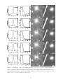
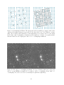
As demonstrated in Fig. 6, the Lanczos4 interpolation function provides the best resampling
for correctly sampled data. In theory one could use an even larger kernel to get a closer-toperfect resampling. However in practice large kernels with a sharply-limited bandpass carry more
problems than advantages. Artifacts, image borders or undersampled data generate extended
ripples (Gibbs’ phenomenon). These ripples are obvious on the saturation trail and the cosmic
ray impact of the Lanczos interpolations in Fig. 6. In addition, the computational cost becomes
prohibitive with multi-dimensional data.
Nearest-neighbour interpolation provides a good conservation of the noise spectrum at scales
close to unity; unfortunately, it generates a terrible aliasing when zooming in, and can distort
a lot object shapes at places. Its usage should therefore be restricted to images such as flag- or
weight-maps.
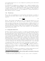
Bilinear interpolation is fast and doesn’t generate negative artifacts. However, it creates a lot of
smoothing by correlating the values of neighbour pixels. On images with white noise, this may
lead to obvious “moiré” effects (Fig. 7). Nevertheless, bilinear interpolation can be useful for
processing undersampled data.
In general, Lanczos3 resampling represents the best compromise. As can be seen in Fig. 8, it
brings a substantial benefit over bilinear interpolation in preserving the signal, while creating
relatively modest artifacts around image discontinuities.
16
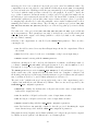
Figure 6: Comparison between resampling methods. From top to bottom: nearest-neighbour,
bilinear, Lanczos2, Lanczos3, Lanczos4. From left to right: Interpolation function profile, Modulation Transfer Function, result from shifting an image by half a pixel in both direction, and
result for a 5× zoom + rotation by 20 degrees.
17
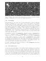
Figure 7: Example of moiré pattern on the background noise, generated by bilinearly resampling
an image containing white noise at a pixel scale slightly different from 1.
5.6.2
Oversampling
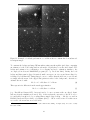
Unfortunately the procedure described above generates aliasing when “zooming out” sufficiently
an image by resampling it at a lower resolution. Moreover, the intensity of the resampled
background white noise stays constant instead of being proportional to the zooming factor
(see Fig. 10). This is because the algorithm essentially decimates the data instead of binning
them within the output pixel footprint: a similar effect applies in the panning windows of
astronomical visualization tools, for instance. This problem can be approximately solved by
dilating appropriately the interpolation kernel, or by pre-filtering the input image (like textures
in 3D hardware). A more exact and more efficient solution is to oversample the output pixel
grid (Fig. 10), in order to obtain a density of samples per unit area (or hypervolume) at least
equal to that of the input image.
Oversampling is controlled by the OVERSAMPLING configuration parameter. If OVERSAMPLING is
set to 1, no oversampling is applied. An OVERSAMPLING of 2 oversamples the data by 2 ndim
samples per pixel, and so on. Oversampling can be different in each dimension: OVERSAMPLING
2,3 will oversample each pixel in a 2 × 3 grid for instance. An OVERSAMPLING of 0 (the default)
lets SWarp select automatically the most appropriate oversampling factor in each dimension,
by comparing pixel scales at the reference point. Although it works fairly well in many cases,
situations where the pixel scale varies a lot over the image — like in all-sky projections — are
not yet properly handled, and manual setting should then be prefered.
Note that oversampling considerably slows down the processing; OVERSAMPLING values should
therefore be selected with some caution!
5.6.3
Noise stability issues
So far we have ignored the influence of noise variations in the resampling process. In theory,
the interpolation schemes described above apply only if the noise is stationary (in the wide
sense) over the extent of the interpolation kernel. Artifacts aside, this can be considered as
true for the background noise, since the weight-maps are reasonably stable at the interpolation
scale. However, the photon noise associated with the sources themselves may vary strongly
over the scale of the PSF FWHM. As most astronomical images are barely oversampled, the
hypothesis of noise stationarity breaks down on bright point sources for which intrinsic photon
18
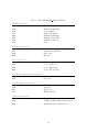
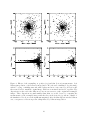
Figure 8: Effects of the resampling on position (top) and flux (bottom) measurements. Left:
bilinear interpolation; right: Lanczos3 interpolation. In both cases, a simulated deep sky image
with 0.7” seeing, containing stars and white background noise, was rotated by 20 degrees and
then rotated back to match the original image. Fluxes were measured in a fixed 2” aperture. The
dispersions seen here reflect the differences between measurements on the original and resampled
images. These dispersions are much smaller than what one would observe by comparing the
measurements on the resampled images with the theoretical (noise-free) positions or fluxes of
the simulation. Note however the significant magnitude offset and flux dispersion in the bilinear
case, consequences of the stronger smoothing induced by bilinear interpolation.
19
Figure 9: Oversampling in SWarp. The input grid is shown as small grey squares, whereas the
output grid (resampled image) is represented by the large tilted ones. Left: Without oversampling, only one interpolation (dark spot) of the input image is done at the center of each output
pixel. Right: with oversampling, several interpolated samples are obtained on a regular subgrid,
and then binned in each output pixel. Here a 3 × 3 oversampling is sufficient.
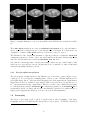
Figure 10: The effect of oversampling in SWarp. A deep, real image with a 0.2” pixel scale
and 0.8” seeing FWHM is resampled at 1” resolution. Left: no oversampling. Right: with 5 × 5
oversampling. Note the lower noise level and higher depth in the right image.
20
noises dominates7 In the most severe cases, resampled noise peaks may generate distorsions in
the resampled profiles.
Low-background-noise simulations were conducted in order to evaluate the amplitude of these
distorsions on correctly-sampled data (PSF FWHM = 3 pixels). The effect is small, although
not totally negligible on sources with intermediate intensity. On profile-fitting measurements
for instance, photometry can be affected at the level of a few millimag rms. The degradation of
astrometric precision was found not to exceed a few millipixels rms. On typical background-noise
limited images the effects are even smaller.
5.6.4
Weight-maps
The processing of the weight-maps (see §5.9.2) follows that of the data images, except that one
is dealing now with variances instead of fluxes. The resampled weight at position x may be
written as
1
w̃(x) = P k2 (x)
(3)
i
i
wi
Therefore when an input weight within the range of the interpolation function is zero, the
interpolated weight is also zero. The general consequence is that the borders of interpolated
images are trimmed by half the range of the interpolation function. Similarly, small “holes” in
a provided weight-map are dilated by the interpolation function footprint. For example, once
interpolated with a Lanczos4 kernel, a single, isolated zero-weight pixel will yield a clump of
about 64 pixels in the resampled image! This is another illustration of the disadvantages in
using large interpolation kernels.
5.7
Background subtraction
The flux at each pixel is a function of the sum of a “background” signal and light coming from
the objects of interest. At most wavelengths, the strongest contribution to the background is of
instrumental/atmospheric/ecliptic origin, and is therefore prone to changes between exposures.
If not subtracted, the compositing of all these exposures will often produce an ugly patchwork
created by all the different individual backgrounds. A solution to this problem is to apply
background-subtraction prior to resampling and co-adding the data. Large-scale gradients of
instrumental origin are commonly found on astronomical images, hence subtracting a constant
from each frame will generally yield poor results, as shown in Fig. 11). It is therefore necessary
to subtract a smooth background map which contains the low-spatial-frequency noise components
of the data, including any offset. Subtracting a background-map may alter or destroy the signal
of scientific interest; thus some caution is needed in choosing parameters for this procedure.
Background subtraction is activated by setting the SUBTRACT BACK configuration parameter to
Y (which is the default). Setting it to N will disable subtraction, but background estimation
will still take place (it is needed by other SWarp tasks), and the processing time will stay
approximately the same.
Background estimation uses SExtractor’s algorithm and is controllable with the same keywords 8 .
The following is largely copied from SExtractor documentation (Bertin 1999).
7
It is possible to stabilize the noise variance using a non-linear dynamic scale transform (Anscombe 1948,
see also Stark et al. 1998). The transformed signal is still bandpass-limited but unfortunately, resampling and
transforming it back biases significantly the data.
8
In SWarp All background configuration keywords accept a list of values, one value for each input frame.
21
Figure 11: Example of residual gradients in a co-addition after a constant has been subtracted
from input images.
To construct the background map, SWarp makes a first pass through the pixel data, computing
an estimator for the local background in each mesh of a grid that covers the whole frame. The
background estimator is a combination of κ.σ clipping and mode estimation, similar to the
one employed in Stetson’s DAOPHOT program (see e.g. Da Costa 1992). Briefly, the local
background histogram is clipped iteratively until convergence at ±3σ around its median; if σ
is changed by less than 20% during that process, we consider that the field is not crowded and
we simply take the mean of the clipped histogram as a value for the background; otherwise we
estimate the mode with:
Mode = 2.5 × Median − 1.5 × Mean
(4)
This expression is different from the usual approximation
Mode = 3 × Median − 2 × Mean
(5)
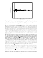
(e.g. Kendall and Stuart 1977), but was found to be more accurate with our clipped distributions, from the simulations we made. Fig. 12 shows that the expression of the mode above
is considerably less affected9 by crowding than a simple clipped mean — like the one used in
FOCAS (Jarvis and Tyson 1981) or by Infante (1987) — but is ≈ 30% noisier. For this reason
we revert to the mean in non-crowded fields.
9
Obviously in some very unfavorable cases (like small meshes falling on bright stars), it leads to totally
inaccurate results.
22
10
Clipped Mode (ADU)
5
0
-5
-10
0
5
10
15
Clipped Mean (ADU)
20
25
30
Figure 12: Simulations of 32 × 32 pixels background meshes polluted by random Gaussian
profiles. The true background lies at 0 ADU. While being slightly noisier, the clipped “Mode”
gives a more robust estimate than a clipped Mean in crowded regions.
The choice of the mesh size (in pixels), BACK SIZE, is critical. If it is too small, the background
estimation is affected by the presence of objects and random noise. But more important is the
fact that part of the flux of extended objects can be absorbed in the background map. The
effect may be almost unnoticeable on individual input images (where the signal-to-noise ratio is
low), and have measurable photometric consequences on the deep, coadded image. It is therefore
advised to use large BACK SIZEs in SWarp. Of course if the mesh size is too large, it will not
be able to reproduce all the variations of the background; a good compromise has to be found
by the user. Typically, for reasonably sampled images, a size of 128 (the default) to 512 pixels
should work well.
The final background map is a (natural) bicubic-spline interpolation between the meshes of the
grid. Before interpolating, a median filter can be applied to suppress possible local overestimations due to bright stars or artifacts. BACK FILTERSIZE sets the size (in background meshes) of
the median filter. “1” means no filtering applied to the background grid. Usually a size of 3
meshes (the default) is sufficient, but it may be necessary to use larger dimensions, especially
to compensate, in part, for small background mesh sizes, or in the case of large artifacts in the
images. Median filtering also helps reducing possible ringing effects of the bicubic-spline around
bright features. In some specific cases it might be desirable to median-filter only background
meshes whose original values exceed some threshold above the filtered-value. This differential
threshold is set by the BACK FILTERTHRESH parameter, in ADUs. The default is 0.
By default the computed background-map is automatically subtracted from the input image.
But there are some situations where it is more appropriate to subtract a constant from the
image (e.g., images where the background noise distribution is strongly skewed). The BACK TYPE
configuration parameter (set by default to “AUTO”) can be switched to MANUAL to allow for
the value specified by the BACK DEFAULT parameter to be subtracted from the input image. The
default value is 0.
As said before, the background estimation procedure is used not only for background subtraction,
23
but also for other tasks in SWarp, such as weight calibration. Thus even if SUBTRACT BACK is
set to N or BACK TYPE is in MANUAL mode, “reasonable” values for other background parameters
must be given to ensure proper working of the software.
Note that the present version of background subtraction doesn’t work on non-2D images.
5.8
Scaling the flux
How are fluxes modified by image warping? Let us assume F is the integrated flux (in units of
e− for simplification) of a source of finite extent S that would be recorded on a perfect detector
array. In the continuous limit, we define
F ≡
Z
S
f (x) d 2x,
(6)
where f (x) is the pixel value at physical position x on the detector. In real life, pixel values are
affected by a variable efficiency q, yielding a measured “raw” flux
Fr =
Z
S
q(x)f (x) d 2x.
(7)
Digital images are generally divided by a “flat-field” and even a “super-flat” prior to SWarping.
The assumption behind flat-fielding is that the light received from the sky or the dome, and
recorded to form the flat-field, has uniform radiance (i.e. constant flux per solid angle). The
flux measured on the flat-fielded image is therefore
Ff =
Z
S
q(x)f (x)
d 2x =
f0 q(x)δΩ(x)
Z
S
f (x)
d 2x,
f0 δΩ(x)
(8)
where δΩ is the local sky area sustained by a pixel (area ≡ 1 in pixel units), and f0 the scaling
factor of the flat-field, which we will set to 1 for the sake of simplicity. As can be seen, flatfielding does not make the image “flat” in terms of sensitivity; it introduces a dependency with
astrometrical distorsion. With most cameras the effect is generally small (≤ 1 millimag). The
resampling operations described in §5.6 are designed to conserve surface brightness per pixel,
hence the flux recorded on the warped image, with new physical coordinates x0 is now
Ff w =
Z
S
f (x) 2 0
dx =
δΩ(x)
Z
S
f (x) ∂x0i 2
dx=
δΩ(x) ∂xj Z
∂x0 i 2
f (x) d x.
∂ξj S
(9)
ξ represents the local (angular) sky coordinate vector. We have made use of the fact that if pixel
size is small compared to the rate of change of plate
scale (which is almost always true), δΩ(x)
∂ξi is equal to the Jacobian of the de-projection ∂xj . Now if an equal-area projection is selected
0
∂x for the output image, ∂ξji is constant and we have the nice relation Ff w ∝ F . This means that
swarping properly flatfielded data using an equal-area output projection produces an image with
a perfectly flat response to the incoming flux10 . This is why equal-area projections should be
prefered to other projections whenever possible.
Immediately following resampling, the intensity of each image is scaled according to the configuration parameters. The flux-scaling parameter pi is the product of two factors: a “photometric”
factor, and an “astrometric” one. Currently, the photometric part must be specified by the
user (for instance in a pipeline it is generally produced by the photometric calibration process).
10
Warning: this flux correction can be extremely inaccurate — 10% error or even more! — for sources that are
undersampled on the output image.
24
The photometric factor can be set directly using the configuration parameter FSCALE DEFAULT:
there must be one value per input image, separated by a coma. It can also be read from the
FITS header. The FSCALE KEYWORD configuration parameter tells SWarp what FITS keyword
to look for in each input image. The default is “FLXSCALE”. If the FSCALE KEYWORD is not
found in the image header, then the FSCALE DEFAULT value is taken instead. FSCALE DEFAULT
is defaulted to 1 for all images.
The astrometric part of the flux-scaling factor corrects for the difference in pixel size between the input and output images. The FSCALASTRO TYPE configuration parameter controls
the behaviour of this “astrometric” flux-scaling. In the current version, the default behaviour
(FSCALASTRO TYPE FIXED) is to apply a constant correction factor to account for possible mismatches in pixel size. Hence flux is conserved only with equal-area projections. “Astrometric”
flux-scaling can also be deactivated by using the FSCALASTRO TYPE NONE option. Future versions
of SWarp may include variable pixel-scale correction for non-equal-area projections.
5.9
Combining resampled images
This is the last part of the processing. Now at each pixel position of the output image, SWarp
has to combine data values coming from all the resampled image, each one coming with a rough
estimate of its variance (from the resampled weight-map). Many combinations are therefore
possible.
5.9.1
Various types of image combination
The user can choose between the following options, as arguments to the COMBINE TYPE configuration parameter:
• AVERAGE: The output is simply an unweighted average of all pixel values with non-zero
weights:
P
pi f i
F = i
,
(10)
n6=0
where pi is the flux scaling factor (see §5.8), and the composite weight is
n26=0
W =P 1 ,
(11)
i qi w i
where the wi are proportional to the inverse of the scaled variance:
1
.
p2i σ 2
Needless to
say that this combination is not optimum in terms of S/N, unless all input images have
identical Gaussian noise.
• CHI2: The output is the square-root of the reduced χ2 of all pixel values with non-zero
weights:
sP
2
i wi f i
.
(12)
F =
n6=0
By construction, the composite weight (the absolute one) is
W ≡ 1.
(13)
The result of the combination is a so-called “χ2 image”. Although it does not respond
linearly to the input signals, it can be used for detecting sources. As shown by Szalay et
25
al. (1999), the “χ2 image” is indeed the optimum combination to achieve panchromatic
detection on a set of images taken at different wavelengths, provided the data sets are
background-noise limited and that the noise is uncorrelated between frames. This assumes
further that the Point Spread Function (PSF) has been homogenized in all channels. χ 2
images are most often used in deep panchromatic surveys requiring photometric redshift
analyses. The double-image mode of SExtractor allows one to detect on the χ2 image
while making the photometric measurements on each of the single-band images.
• MEDIAN: The output is the median of all scaled pixel values with non-zero weights:
F = median(fi ).
(14)
Assuming Gaussian noise distribution, we obtain the following approximation to the composite weight (see e.g. Kendall & Stuart 1977):
 P √ 2
wi

i

n6=0 + π2 − 1 if n6=0 is even,
 π2
n6=0
P √ 2
W =

wi

i
 2
(n6=0 + π − 2) otherwise.
π
n
(15)
6=0
This approximation can become inaccurate if wj varies by large proportions (a factor of
3 or more) from frame to frame. The median is convenient for combining data polluted
by unidentified glitches or noise spikes. It generally provides “safe” (robust) co-additions
even with strongly non-Gaussian noise distributions. However it is suboptimal for Gaussian
noise: the resulting variance is increased by ≈ 60% compared to what is obtained with
an average. As with all non-linear combinations, one should check that input images have
approximately the same Point Spread Function if point-sources are to be co-added.
• MIN: The output is the minimum of all pixel values with non-zero weights:
F = min(pi fi ).
(16)
The variance of F is too “noise-distribution dependent” to allow some estimation, hence
we set
(
1 if n6=0 6= 0,
(17)
W =
0 otherwise.
• MAX: The output is the maximum of all pixel values with non-zero weights:
F = min(pi fi ).
(18)
The variance of F is too “noise-distribution dependent” to allow some estimation, hence
we set
(
1 if n6=0 6= 0,
(19)
W =
0 otherwise.
Maxima and minima can be useful for identifying defects or rare events in a set of data.
• WEIGHTED: The output is a weighted average of input values:
P
i w i pi f i
F = P
.
i wi
(20)
The output weight is just the sum of input weights:
W =
X
wi .
(21)
i
This combination should be the most appropriate for detecting and measuring faint sources
on properly weighted, homogeneous images. Because it is a linear processing, new data
can be added later if needed.
26
5.9.2
Weighted coaddition
Weight-maps provide a convenient way to store the standard flux error assigned to each pixel.
For each input image 1 ≤ i ≤ N entering image combination, one can define the following
parameters in an arbitrarily small “pixel” j:
- The local, uncalibrated flux fij = fij + ∆fij , where fij is the flux contributed by the sky
background, and ∆fij that contributed by celestial sources,
2 = σ 2 + ∆σ 2 , where σ 2 is the flux variance
- the local, uncalibrated variance of the flux σij
ij
ij
ij
2 that contributed by the photon statistics
contributed by the background noise, and ∆σij
of celestial sources,
- the local,normalized weight11 wij ,
- the electronic gain of the CCD gi , in e− /ADU (defined at wij = 1),
- the relative flux scaling factor pi deduced from the photometric solution to calibrate the
images:
pi ∆fij = pl ∆flj ∀ i, j, l,
(22)
- and the relative weight scaling factor qi derived from the comparison of the background
noise level with the normalized weight; input images will be weighted with qi wi .
∆fi , ∆σi2 , wi and gi are related through:
gi wij =
∆fij
2 .
∆σij
(23)
Now, to optimally co-add calibrated images, one could weight them using
qi wij =
1
2 .
p2i σij
(24)
However, such weight maps exhibit strong variations on small scales, in the presence of celestial
2 increases a lot on bright pixels). The modulating effect of weighting, combined
objects (σij
with variations of the PSF and sampling errors would lead to significant distorsions of stellar
profiles. It is therefore more appropriate to weight pixels according to the intensity of the local
background noise, which is far smoother:
qi wij =
1
2
p2i σij
.
(25)
This has also the advantage that one can use normalized flat-fields as wij ’s, without prior
knowledge of the CCD gain in the case where instrumental noise is negligeable. For faint
objects, this weighting scheme is as efficient as that of (24), and is only suboptimum for the
objects with very high surface-brightness, when the qi ’s vary a lot from exposure to exposure.
But as these objects are easily detected on individual exposures, the most accurate photometry
is still possible by combining the N measurements.
11
Both fluxes and weights may have gone through resampling, but for the sake of clarity we shall from now
drop the “ ˜ ” from §5.6
27
In practice, SWarp can read several types of weight-maps, although they are all internally
converted to variance for processing. The input weight-map format must be specified with the
WEIGHT TYPE keyword. WEIGHT TYPE NONE is for no input weight-map (the default), MAP RMS for
indicating that the data contain the absolute standard deviation of pixel values, MAP VARIANCE,
for weight-map data stored as relative variances, and MAP WEIGHT for relative weights. Relative
variances or weights are scaled internally using local variance measurements made directly on
the input images.
When producing composite fields larger than the input images, the latter must be backgroundsubtracted prior to coaddition, to avoid generating discontinuites in the output image. Thus
one can write the output coadded flux as
∆fj =
P
i qi wij pi ∆fij
and the resulting variance as
∆σj2
P
=
i qi wij
P
= pl ∆flj ∀l,
2
2 2 2
i ki wij pi ∆σij
.
P
( i qi wij )2
(26)
(27)
Using (23), an equivalent “local gain” Gj in the coadded image can be computed:
P
X
∆fj
i qi wij pi ∆fij
P
G j wj =
=
qi wij ,
.
2
2 2 2
∆σj2
i ki wij pi ∆σij
i
(28)
where wj is the composite weight-map of the coadded image. From our definition of weights,
wj is inversely proportional to σj2 and must be 1 if all input weights are at 1; hence it is easy to
show that
P
i qi wij
wj = P
.
(29)
i qi
Substituting (29) in (28), and using (22) and (23), one gets
Gj = P
P
X
i qi wij
−1 .
2
i ki wij pi gi
i
qi .
(30)
Unfortunately, as can be seen, this “coadded gain” will vary with position in the general case.
Nevertheless, some approximations can be made to simplify this expression. First of all, in most
cases, gi will be almost constant from one input image to another. Second, if exposures are
taken under photometric conditions with constant sky brightness and negligible instrumental
noise, one should have qi ∝ p−1
i , removing the dependence with input weights, and therefore
position in the coadded image. In that very case, the resulting gain is simply
G≈g
X
p−1
i .
(31)
i
Sadly, in many bands, the presence of clouds does not decrease the sky brightness as much
as source brightness, and doesn’t act at all like a decrease in global sensitivity or exposure
time. Coadded regions of a survey that are taken under non-photometric conditions experience
fluctuating “gains”. But this effect is generally small: taking the quite unfavourable case of
qi ∝ p−2
(constant background noise) with pi ’s varying by a factor of 4 between two exposures,
i
and weights varying from 0.5 to 1, makes Gj to vary by 20% at most. This should not cause
significant difficulties in any profile fitting routine. Therefore (31) still remains a very good
approximation in the general case, and the “coadded gains” provided by this method are still
more stable than what unweighted co-addition offers.
This does not prevent regions with lower coverage (in which N is smaller) having lower gains. To
avoid large gain drops in the gaps of CCD mosaic images, it is recommended for the observations
to use large, random dithering patterns consisting of at least 4-5 exposures per covered sky area.
28
5.9.3
Image buffering and memory constraints
In order to maximize the efficiency of the image combination process, SWarp version 2.0 and
above allocates a significant amount of memory to buffer input and output data. This amount
of memory can be set by the user with the COMBINE BUFSIZE configuration parameter. The
default value for COMBINE BUFSIZE is 64 (Megabytes). If your machine is a bit short of memory
you should decrease this value. Conversely if you need to combine a large number of overlapping
images, you might want to set COMBINE BUFSIZE to a substantial fraction of the memory available
on your machine to avoid “disk thrashing”.
6
Two-step co-addition and resampling
All the operations described so far can be done in one single run of SWarp. This generally
sufficient for small projects, which usually involve observations conducted over a short period
of time. However, for large sky surveys that can extend over years, this implies “waiting” for
the data to accumulate after passing through the reduction pipeline. In this case SWarp would
only be started once all the fields that cover a given sky area are available. Much of SWarp
processing time is spent in resampling the data; therefore for projects that extend over a long
period of time, it would be more efficient to resample the images as they come out of the
reduction pipeline. The remaining of the work, co-addition, could be done at a later date.
To solve this problem, versions ≥ 1.32 of SWarp allow the internal processing pipeline to be
split in two: image-resampling and image-combining. If the COMBINE configuration parameter
is set to N, SWarp stops right after having background-subtracted and resampled the input
images. The DELETE TMPFILES option is then automatically deactivated.
To combine images resampled at an earlier stage, RESAMPLE should be set to N: in that case
SWarp will skip all the background-subtraction and resampling stage, and jump directly to the
combine process. Prior to version 2.0 this feature only worked with input resampled images
produced by SWarp, because of some specific information needed in the FITS header. Since
version 2.0, any FITS image can be used. However, when RESAMPLE is set to N, SWarp combines
input images with the implicit assumption that they all share the same CRVAL and CDELT WCS
parameters: images are placed in the final frame according to their CRPIX and NAXIS.
Setting both RESAMPLE and COMBINE to N will not produce any output file, but can be useful
to check the content of input data or to adjust output astrometric parameters. By default,
RESAMPLE and COMBINE are both set to Y.
It may sometimes be useful to create only the header of what will become the combined image;
for instance for generating an output “.head” file that will define the output projection system.
Such a “.head” file can then be copied to several machines that will resample input images
to a common projection, for later co-addition. This can be done by setting the HEADER ONLY
configuration parameter to Y; processing will stop before resampling like in the case where
RESAMPLE and COMBINE are set to N, but this time the header of the output image will be written
to disk.
7
Examples
In the following, examples of use of SWarp are given, together with commented configuration
files.
29
7.1
Example 1
Let us assume one wants to produce a full-sky Aitoff representation in galactic coordinates of a
series of observed fields stored in *.fits 2D files( with WCS info), for illustration purposes. The
files might be dummy ones, supplemented with hand-made headers, or obtained from virtual
telescopes such as SkyView12 , or real ones. In all cases an additional full sky map is useful to
delimit the full-sky: one may for instance download a 360 degrees Aitoff projection of COBEDIRBE data from SkyView. The syntax is
%
swarp
*.fits
A possible default.swarp configuration file is
#---------------------------------- Output -----------------------------------IMAGEOUT_NAME
WEIGHTOUT_NAME
coadd.fits
coadd.weight.fits
#------------------------------- Input Weights -------------------------------WEIGHT_TYPE
WEIGHT_SUFFIX
WEIGHT_IMAGE
MAP_WEIGHT
.weight.fits
# Not used here
#------------------------------- Co-addition ---------------------------------COMBINE_TYPE
AVERAGE
# This coaddition is for illustration
# only: the weight-map will contain
# a sum of field footprints
#-------------------------------- Astrometry ---------------------------------CELESTIAL_TYPE
PROJECTION_TYPE
CENTER_TYPE
CENTER
PIXELSCALE_TYPE
PIXEL_SCALE
IMAGE_SIZE
GALACTIC
#
AIT
#
MANUAL
#
00:00:00.0, +00:00:00.0 #
MANUAL
#
#
1800.0
#
#
800,400
#
#
Coordinate system forced to galactic
Code for Aitoff
Imposed to alpha = delta = 0.0
The full sky area will exceed the
fraction that contains the fields
in arcsec: Half a degree per pixel
at image center, on both axes
360/0.5 = 720, 180/0.5 = 360,
plus a margin
#-------------------------------- Resampling ---------------------------------RESAMPLING_TYPE BILINEAR
OVERSAMPLING
4
INTERPOLATE
N
12
#
#
#
#
http://skyview.gsfc.nasa.gov
30
For illustration purposes, no need
for a sophisticated interpolation
A small oversampling only to have
pretty, antialiased field limits
GAIN_KEYWORD
GAIN_DEFAULT
GAIN
0.0
#--------------------------- Background subtraction --------------------------SUBTRACT_BACK
BACK_TYPE
BACK_DEFAULT
BACK_SIZE
BACK_FILTERSIZE
N
AUTO
0.0
128
3
# No background subtraction
#------------------------- Virtual memory management -------------------------VMEM_DIR
VMEM_MAX
MEM_MAX
.
2047
128
# 128 MB should be enough to avoid
# swapping
#------------------------------ Miscellaneous --------------------------------DELETE_TMPFILES Y
VERBOSE_TYPE
NORMAL
# Delete temporary resampled FITS files
In this application, coverage maps can be generated using the output weight-map instead of the
image itself.
7.2
Example 2
In this example, one has a set of CCD images taken with a standard dithering strategy,
input*.fits, and the related set of weight-maps input*.w.fits However the unusual thing
is that for some reason the output has to be tilted by 30 degrees with respect to the local
north-south axis, and the pixels must have an aspect ratio of 16:9!
First, one starts with a fairly standard configuration file:
#---------------------------------- Output -----------------------------------IMAGEOUT_NAME
WEIGHTOUT_NAME
coadd.fits
coadd.weight.fits
# Output filename
# Output weight-map filename
#------------------------------- Input Weights -------------------------------WEIGHT_TYPE
MAP_WEIGHT
WEIGHT_SUFFIX
WEIGHT_IMAGE
.w.fits
#
#
#
#
#
(all or for each weight-map)
Suffix to use for weight-maps
Weightmap filename if suffix not used
(all or for each weight-map)
#------------------------------- Co-addition ---------------------------------COMBINE_TYPE
WEIGHTED
# weight-maps are provided
31
#-------------------------------- Astrometry ---------------------------------CELESTIAL_TYPE
PROJECTION_TYPE
CENTER_TYPE
CENTER
PIXELSCALE_TYPE
PIXEL_SCALE
IMAGE_SIZE
NATIVE
# Standard stuff
TAN
# A tangent projection will do
ALL
# We want all the data to fit in
00:00:00.0, +00:00:00.0 # Not used in CENTER_TYPE ALL mode
MEDIAN
# Will be overriden by coadd.head
0.0
# Not used in MEDIAN mode
0
# Automatic sizing
#-------------------------------- Resampling ---------------------------------RESAMPLING_TYPE
OVERSAMPLING
INTERPOLATE
GAIN_KEYWORD
GAIN_DEFAULT
LANCZOS3
0
N
GAIN
0.0
# High quality resampling
# Auto. oversampling (=1 in that case)
#--------------------------- Background subtraction --------------------------SUBTRACT_BACK
BACK_TYPE
BACK_DEFAULT
BACK_SIZE
BACK_FILTERSIZE
Y
AUTO
0.0
128
3
# Needed for co-adding dithered fields
#------------------------- Virtual memory management -------------------------VMEM_DIR
VMEM_MAX
MEM_MAX
.
2047
128
# 128 MB should be enough to avoid
# swapping
#------------------------------ Miscellaneous --------------------------------DELETE_TMPFILES Y
VERBOSE_TYPE
NORMAL
# Delete temporary resampled FITS files
To implement the unusual output features required, one must write a coadd.head ASCII file
that contains a custom anisotropic scaling matrix. A coadd.head for pixels 0.2” large, that tilts
the image by 30 degrees and applies a 16:9 anamorphosis to the data would be:
CD1_1
CD1_2
CD2_1
CD2_2
END
= 6.4150E-5
= 2.0833E-5
= -3.7037E-5
= 3.6084E-5
32
8
Troubleshooting
My window terminal crashes during a long SWarp run!
Unexpected crashes of XTerm windows have been reported. This seems to be caused by the
large number of ANSI control sequences that SWarp sends to the terminal. You may either set
the SWarp configuration keyword VERBOSE TYPE to QUIET or FULL, and/or redirect the output
to a file.
SWarp crashes with error messages like “> *Error*:
pthread create() failed...”.
The multithreaded version of SWarp requires a fairly large stack, that may exceed the maximum
value allowed by your shell. Use the shell command limit to increase the stacksize parameter
if required (you might need the root privileges to change this if it is a “hard” limit).
SWarp crashes with error messages like “> *Error*: Not enough memory for...”,
although I have properly set the MEM MAX VMEM MAX parameters.
The maximum value allowed by your shell for memory use might be set too low. Use the shell
command limit to increase the datasize, memoryuse and vmemoryuse parameters if required
(you might need the root privileges to change this if it is a “hard” limit).
SWarp crashes with error messages like “> *Error*: cannot open for reading...”
during the co-addition phase, although it had no problem accessing the same files
for resampling.
The maximum number of open files allowed by your shell might be set too low. Use the shell
command limit to increase the descriptors and openfiles parameters if required (you might
need the root privileges to change this if it is a “hard” limit).
9
Acknowledgements
Many thanks go to Mark Calabretta (ATNF/CSIO, Epping) for his great astrometric library,
Nicolas Devillard (ESO, Garching) for introducing me to memory-mapping techniques, Mireille
Dantel-Fort, Laurent Domisse, Frédéric Magnard, Yannick Mellier (TERAPIX/IAP), Mario
Radovich (OAC, Naples), Roeland Rengeling (Sterrewacht, Leiden), Roy Williams (CACR, CalTech) and Dafydd Wyn Evans (IoA, Cambridge) for extensive testing and suggestions, and Henry
Joy McCracken (TERAPIX/IAP) for help with the manual and additional testing.
References
[1] Anscombe F.J., 1948, Biometrika 15, 246
[2] Bertin E., 1999, SExtractor 2.1, User’s manual, IAP
[3] Da Costa G.S., 1992, in Astronomical CCD Observing and Reduction Techniques, ed. Howell S.B. (ASP Conf. Series)
[4] Fruchter A., Hook R.N., 1997, SPIE 3164, 120
[5] Infante L., 1987, A&A 183, 177
[6] Jarvis J.J., Tyson J.A., 1981, AJ, 86, 476
33
[7] Kendall M., Stuart K., 1977, The Advanced Theory of Statistics, Vol. 1, (Charles Griffin
& Co., London)
[8] Starck J.-L., Murtagh F., Bijaoui A., 1998, Image Processing and Data Analysis (Cambridge
University Press)
[9] Szalay A.S., Connolly A.J., Szokoly G.P., 1999, AJ 117, 68
[10] Wolberg G., 1992, Digital Image Warping (IEEE Computer Society Press)
34