
1
FACULTY OF TECHNOLOGY
Application Software Development via Model Based
Design
Olli Haapala
Master´s Thesis
Department of Process and Environmental Engineering
May 2014
ABSTRACT
FOR THESIS
University of Oulu Faculty of Technology
Degree Programme (Bachelor's Thesis, Master’s Thesis)
Major Subject (Licentiate Thesis)
Master’s Thesis
Author
Thesis Supervisor
Haapala Olli
Sorsa A (D.Sc), Leiviskä K (Prof.)
Title of Thesis
Application Software Development via Model Based Design
Major Subject
Type of Thesis
Submission Date
Number of Pages
Process automation
Master’s Thesis
May 2014
71
Abstract
This thesis was set to study the utilization of the MathWorks’ Simulink® program in model based application software
development and its compatibility with the Vacon 100 inverter. The target was to identify all the problems related to
everyday usage of this method and create a white paper of how to execute a model based design to create a Vacon
100 compatible system software.
Before this thesis was started, there was very little knowledge of the compatibility of this method. However during
the practical experiments, it became quite quickly clear that this method is very compatible with the Vacon 100.
Majority of the problems expected before this thesis was started proved to be wrong. The only permanent problem
that came up during this thesis was that Vacon 100 supports only the 32-bit floating-point precision while Simulink
uses the 64-bit floating-point precision by default.
Even though this data type incompatibility prevents usage of some of the Simulink’s blocks, it is by no means a
limiting factor that restricts usage of this method. During the practical research no problems were found that
completely prevent the usage of this method with the Vacon 100 inverter.
The Simulink PLC Coder was in the spotlight during the practical research work. Even though the code generator
worked better than was expected, the biggest problems limiting the usage of model based design relates to the PLC
Coder.
All in all based on this study, it is easy to say that model based design is a very usable tool for everyday design work.
The method does not necessarily show its advantages in a small scale design work and the implementation phase can
take some time before the company has collected the support model library needed. However in the future, the
software requirements will increase, which grows the importance of model based design. A well-executed model
based design can have a significant improving effect on financial, time and quality aspects.
Additional Information
TIIVISTELMÄ
OPINNÄYTETYÖSTÄ
Koulutusohjelma (kandidaatintyö, diplomityö)
Oulun yliopisto Teknillinen tiedekunta
Pääaineopintojen ala (lisensiaatintyö)
Diplomityö
Tekijä
Työn ohjaaja yliopistolla
Haapala Olli
Sorsa A (TkT), Leiviskä K (Prof.)
Työn nimi
Application Software Development via Model Based Design
Opintosuunta
Työn laji
Aika
Sivumäärä
Automaatiotekniikka
Diplomityö
Toukokuu 2014
71
Tiivistelmä
Tämän lopputyön tarkoituksena oli tutkia MathWorks:n Simulink®-ohjelmiston käyttöä mallipohjaisessa
ohjelmistotuotannossa ja sen soveltuvuutta Vacon 100 -taajusmuuntajan ohjelmointiin. Tavoitteena oli identifioida
kaikki ongelmakohdat, jotka vaikuttavat menetelmän jokapäiväisessä hyödyntämisessä, sekä luoda raportti, miten
menetelmän avulla voidaan tehdä Vacon 100 yhtensopiva ohjelmisto.
Ennen työn aloittamista menetelmän soveltuvuudesta ei ollut tarkkaa tietoa. Työn aikana suoritetut käytännönläheiset
ohjelmistotuotantoesimerkit kuitenkin osoittivat nopeasti menetelmän toimivuuden. Ongelmakohdat, joita ajateltiin
ennen työn aloittamista, osoittautuivat pääosin vääriksi. Ainoa pysyvä ongelmakohta, joka työn aikana tuli esille, on
Vacon 100:n tuki vain 32-bit reaaliluvuille, kun taas Simulink käyttää oletuksena 64-bit reaalilukua.
Vaikka datatyypistä aiheutuva ongelma estääkin muutaman Simulink-lohkon käytön, se ei kuitenkaan ole
menetelmän käyttöä rajoittava ongelma. Työssä ei tullut vastaan yhtään ongelmaa, joka olisi estänyt mallipohjaisen
suunnittelun käytön Vacon 100 -laitteen kanssa.
Simulink:n koodigenerointityökalu eli Simulink PLC Coder on tärkeässä osassa työn tutkimuksen kannalta.
Kaikenkaikkiaan koodigeneraattori toimi yli odotusten, mutta suurimmat ongelmat, jotka rajoittajavat mallipohjaisen
suunnittelun käyttöä, liittyvät kuitenkin PLC Coder:n toimintaan.
Yhteenvetona työn perusteella voidaan todeta, että mallipohjainen ohjelmistotuotanto on nykyaikana erittäin
käyttökelpoinen menetelmä. Tosin menetelmän tuomat hyödyt eivät välttämättä tule esille pienessä mittakaavassa ja
ennen kuin yritykselle on muodostunut omaan tuotteeseen liittyvien mallien ja lohkojen tietokanta. Tulevaisuudessa
kuitenkin suunnittelutyön vaatimusten kasvaessa, mallipohjaisen ohjelmistotuotannon merkitys tulee kasvamaan.
Hyvin toteutettuna menetelmä parantaa huomattavasti suunnittelutyön tulosta niin taloudellisesti, ajallisesti kuin
laadullisestikkin.
Muita tietoja
PREFACE
This thesis is made for Vacon Oyj and the target for this study is to research if the model
based design method can be utilized in everyday design work. The main goal is to look
this subject from a third party point of view and study if the method could be used by a
person without any PLC programming background.
T
y
This thesis was carried out in the University of Oulu with a close cooperation with theö
Vacon Oyj personnel. There were many people from different departments along then
entire study. I want to say a big thanks to all of you. If there were any problems during
this thesis, I got always help and without all of you this thesis would have been muchT
harder to conduct.
e
k
I want to say a special thanks to Hannu Sarén, the Chief Research Engineer at Vacon Plc.
i
Without Hannu this thesis wouldn’t have come true. The last thanks I want to hand out
j
belongs to Aki Sorsa, the Postdoctoral researcher in the University of Oulu and the
ä
supervisor for this thesis.
Oulussa, 15.5.2013
Olli Haapala
TABLE OF CONTENTS
1 Introduction .................................................................................................................... 7
2 IEC 61131-3 ................................................................................................................... 8
2.1 Introduction ............................................................................................................. 8
2.2 Structure .................................................................................................................. 9
2.2.1 Common elements ......................................................................................... 9
2.2.2 Programming languages .............................................................................. 12
2.3 Benefits and disadvantages ................................................................................... 15
3 Model Based Design .................................................................................................... 16
3.1 Software development process .............................................................................. 16
3.2 Advantages of model based design ....................................................................... 19
3.3 Drawbacks ............................................................................................................. 21
4 MATLAB® .................................................................................................................. 24
4.1 Simulink ................................................................................................................ 24
4.2 Simulink PLC Coder ............................................................................................. 25
5 Modeling of a system ................................................................................................... 27
5.1 Definition of a model ............................................................................................ 27
5.2 The basic principles for creating a model ............................................................. 28
5.3 Modeling methods and tools ................................................................................. 29
6 PLC application software development example ......................................................... 32
6.1 System requirements ............................................................................................. 33
6.2 Modeling the target system ................................................................................... 33
6.2.1 Mathematical model .................................................................................... 33
6.2.2 Graphical model........................................................................................... 36
6.2.3 Verification of the model ............................................................................. 38
6.3 Model based design ............................................................................................... 40
6.3.1 Verification of the design ............................................................................ 42
6.4 Preparing the design for code generation .............................................................. 42
6.5 Code generation and import to IDE ...................................................................... 44
6.6 Integrating the imported code into the system software ....................................... 45
7 Improving the design.................................................................................................... 49
7.1 Introduction for efficient design techniques ......................................................... 49
7.2 Simulink PLC Coder ............................................................................................. 50
7.2.1 Code generation verification........................................................................ 50
7.2.2 Automatic documentation tools ................................................................... 51
7.2.3 Code optimization........................................................................................ 53
7.3 Simulink tools ....................................................................................................... 55
7.4 System software development............................................................................... 56
7.4.1 Accessory blocks ......................................................................................... 56
7.4.2 Example of an accessory block.................................................................... 57
8 Limitations and things to consider ............................................................................... 59
8.1 Simulink PLC Coder ............................................................................................. 59
8.1.1 Block restrictions ......................................................................................... 59
8.1.2 MATLAB functions..................................................................................... 60
8.1.3 Multiple task execution time levels ............................................................. 62
8.2 Vacon 100 ............................................................................................................. 65
8.3 Problems during the code implementation process ............................................... 67
9 CONCLUSIONS .......................................................................................................... 68
10 REFERENCES........................................................................................................... 70
7
1 INTRODUCTION
Traditionally the software development process has relied strongly on sketching the
design into a paper and hand writing it into a software code. It is still the most popular
way to produce a system software. Nowadays though the software requirements have
increased so much that in the traditional software development method the timespan
between the design and the design verification can be months or even years.
This is a big problem and in the future it will only get worse, because the computing
power increases all the time, which means that the software requirements increases all the
time. This thesis was set to study the possibility to use simulation as a tool, instead of
hand coding and hardware based testing. The method in question is called model based
design.
The target for this thesis is to study if the model based design method could be used to
create a system software for the Vacon 100 inverter. There is very little background study
on this subject and it is clear that, like in any new method, there will be some problems
on the way. The question is that will these problems be lethal and is there any reasonably
way to utilize this method in everyday design tasks.
This thesis contains a total of 9 chapters to give a reader an idea of what does the model
based design method mean and how it is executed. The first chapters introduce the reader
to the theoretical aspect of the model based design method starting with an introduction
to the IEC 61131-3 standard. This is a very important chapter and even though model
based design is basically code free programming, it is still important to understand the
basic structure of the PLC. After this chapter there is an introduction to the model based
design method and the related MATLAB tools.
After the theoretical part the thesis has a white paper style introduction to the model based
design work in chapter 6. It shows the reader an example of how to execute a model based
design work. Chapters 7 and 8 show how to success with the model based design method
and take the design into the next level. The last chapter discusses issues noted during this
thesis and gives some future perspectives this method has.
8
2 IEC 61131-3
The IEC 61131-3 is the third part of the IEC 61131 standard for programmable logic
controllers (PLC). This chapter gives a short introduction to the standard, so the reader
can understand the basic structure of the IEC 61131-3 programming language and
terminology related to the subject.
2.1 Introduction
The IEC 61131 standard is divided into 8 parts, containing all the necessary hardware and
software requirements for creating a standard compliant PLC system. This thesis
concentrates only on part 3, which is programming languages. Part 3 or more commonly
known as the IEC 61131-3 is the first successful vendor independent programming
language standard for PLC environment.
The standard was originally developed, because traditional programming techniques had
reached their limits in process environments with constantly increasing complexity. Also
increased processor capacity had opened doors for new programming methods. Before
this standard was developed, every PLC manufacturer used their own programming
method. This was very challenging from user’s point of view and limited PLC markets.
One of the key criteria for this standard was to create an unambiguous and truly
manufacturer independent programming language that adapts to the previously used
languages. (John & Tiegelkamp, 2010)
The development of the IEC 61131-3 standard started in 1979 and the first draft was
completed in 1982. The first official version was published in 1993. Since then it has been
revised twice in 2003 and 2013. Before the IEC 61131-3, there have been several attempts
to create a universal standard for PLC programming, but the IEC 61131-3 was the first
attempt that received the necessary international recognition. This is mostly due to that
the standard was developed in close cooperation with main PLC manufacturers and they
did not try to create a completely new programming technique. The IEC 61131-3 is more
like a combination of well-proven and commonly used programming techniques. (John
& Tiegelkamp, 2010)
9
2.2 Structure
The easiest way to study the IEC 61131-3 standard is by splitting it into two parts: the
common elements and programming languages.
2.2.1 Common elements
The common elements can be thought as a platform of the standard. They include all the
necessary base elements that does not depend on the programming language. Figure 1
shows some of these common elements and the basic structure of a standard compliant
PLC system. At the highest level there are the configuration elements and a configuration.
A configuration is an element that joins together all the resources. In a real world
implementation a configuration can be thought as a PLC rack, which enables different
PLCs to communicate together. Each configuration must include at least one resource.
A resource is a processing unit that is able to execute standardized code. In real world, a
resource can be thought as a processor of the PLC unit, which is driven by one or more
tasks. A task is an element that orders a program execution. For each executed program
or function block, there must be a task that refers to it. Tasks can be executed either
periodically with a chosen interval or they can be configured to execute by cause of a
trigger, for example change of a variable. Traditionally PLCs are configured so that there
is only one resource and one task that drives one program. Nowadays with increased
processor capacity and standardized programming methods, it is much more common to
create several tasks with each task running multiple programs (ABB, 2007). (John &
Tiegelkamp, 2010)
10
Figure 1. The common elements of IEC 61131-3 standard. The figure is based on (John
& Tiegelkamp, 2010: 234, 236).
While the configuration elements create the hardware base of PLC programming, the
program organization units (POU) form the software part. One of the main design targets
for the IEC 61131-3 standard was to unify and simplify POU types. This resulted in the
standard that corresponds to three types of POU: a program, a function block and a
function. The function (FUN) is a so called base POU without any inner state, which
means that the output value depends only on its input value. There are many standardized
functions specified in the IEC 61131-3 standard, for example ADD, ABS, SIN and SQRT.
Also the PLC manufacturers often add their own functions beside the standard functions.
The function block’s (FB) value depends also on the state of its internal (VAR) and
external (VAR_EXTERNAL) variables. In other words, beside an algorithm, the FB
contains also data values. The FB is the most commonly used POU type. One reason for
this is its reusability. Ready-made FBs can be utilized as many times as needed and they
11
can be even used in different programs or different projects. At the highest level of the
POU hierarchy, there is the program (PROG) block. It is considered as the main POU,
because it can communicate with hardware I/O-variables. The FUN and the FB are
considered as basic building blocks and the PROG is the platform to combine them and
create a functional entity. (John & Tiegelkamp, 2010), (ABB, 2007)
Variables are a big part of communication between POUs. There are four basic types of
variables: local, input/output, external and global variables. In figure 2 a block diagram
is sketched to show a typical way to use these variables.
Figure 2. An example of how the different variables could be utilize.
The local variables (VAR) are only available inside one POU and cannot be used or seen
outside of it. The input and output variables are used to bring value data to and from a
POU. The input and output variables are not passed as variables. They just provide a value
transfer channel between POUs under a Program block. For communicating between the
Program POUs, there are global variables inside a resource. The global variables are a
very important part of the software, because they are also used to communicate with
hardware I/Os. Transferring of data between global variables and POUs occurs via
external variables. In other words a global variable is available only for POUs that list it
as an external variable. It means that every external variable needs a corresponding global
variable in Program. (John & Tiegelkamp, 2010)
Other variable types include for example access paths and directly represented variables.
From POU’s point of view the access paths work very similarly as the global variables,
but whereas the global variables are valid in one configuration, the access paths are
intended for communication between configurations. Communication between PLCs is
defined more precisely in the IEC 61131-5 standard. Another data exchange path is to use
12
directly represented variables. A directly represented variable is basically an indication
straight to the PLC hardware address. It is not really designed to be used for
communication between different parts, but in theory it is possible. In table 1, there is an
overview of different communication methods between the common elements shown in
figure 1. (John & Tiegelkamp, 2010)
Table 1. Communication boundaries between different configuration elements and
POUs. (John & Tiegelkamp, 2010)
2.2.2 Programming languages
The IEC 61131-3 standard consists of five different programming languages: one upper
level structure language, two textual languages and two graphical languages. In figure 3
an example of each one these languages is presented. These examples are made with the
MULTIPROG® software.
Figure 3. An example of each one of the IEC 61131-3 programming languages.
Structured text (ST) is a very powerful, high level programming language that resembles
closely to Ada, PASCAL and C languages from the PC world. Nonetheless it is designed
specifically for PLC programming. ST is a very popular language amongst programmers
13
due to its connections to other programming languages and similar structures such as for,
if, while and case structures. Although there are some restrictions to ensure stability, like
the jump structure (GOTO), ST is a very clearly constructed and fairly compact language.
The basic structure of ST consists a number of steps, called statements, and each
statement ends with a semicolon (;). To help readability, it is possible to add comments
with (* comments *) syntax in any part of the statement, where spaces are allowed. The
ST code is also quite similar to Matlab code and there is a comparison between these two
later in this thesis at the page 62. (John & Tiegelkamp, 2010)
Function block diagram (FBD) is a graphical language that originates from signal
processing. Over the years it has increased its popularity, escpecially in process industry,
and that is why it has become a widely accepted language also in the PLC world. Instead
of textual code, FBD has visual networks, where graphical coding element blocks are
connected together with lines. This means that it is visually very explicit and easy to
understand and therefore suitable ecpecially for higher level Program blocks. Execution
in FBD language is carried out from top to bottom, network by network. If it is necessary,
then the order can be manipulated with jumps and returns. (John & Tiegelkamp, 2010)
Ladder diagram (LD) has a bit similar principles as FBD. It uses networks that are
executed from top to bottom, unless user specifies otherwise. LD originated in the USA
and it is based on graphical presentation of relay ladder logic (ABB, 2007). It reminds a
typical electrical circuit diagram, so it is therefore very easy to understand, ecpecially for
people with some kind of eletrical background. LD is mainly designed for describing a
boolean type signal flow from left to right. The base network consists a so called power
trail, where all the logical components are placed. The logical components can either pass
or interrupt the signal flow. If all the components pass the signal then the end result is 1
(TRUE), if not then it is 0 (FALSE). (John & Tiegelkamp, 2010)
Instruction list (IL) is European answer for ladder diagram. It resembles closely the lowlevel assembly language (ABB, 2007). The basic instruction list command has at least
two elements: operator/function and operand. One line represents one command, so it is
a line-oriented language with execution order from top to bottom excluding possible
jumps. The IL language also accepts same kind of comment syntaxes as the ST language.
(John & Tiegelkamp, 2010)
14
Sequential function chart (SFC) is usually considered more as an upper level technique
to describe the sequential behavior of a control software. In the IEC 61131-3 standard
SFC was designed for breaking down complex systems into smaller elements while
giving a user an overall picture of the system. These elements can be programmed in any
of the IEC languages, including SFC, but in lower level SFC is generally used only to
solve quite simple problems. SFC originates from Petri Nets and the IEC 848 Grafcet
languages.
The basic structure of SFC consists transitions, action blocks and steps. When the
transition is true, then the next step is activated with related action blocks. Overall SFC
is quite straightforward, where each step represents a specific part of the process as shown
in figure 4. It is especially suitable for processes with clear step by step behaviour, for
example a batch process.
Figure 4 Sequential Function Chart.
One of the biggest reasons that makes this standard so popular is that POUs can be
programmed in any of the standard’s languages. For example a function can be
programmed in different language than the function block that calls it. In most cases
function blocks can be even coded in C language (ABB, 2007). (John & Tiegelkamp,
2010)
15
2.3 Benefits and disadvantages
The IEC 61131-3 standard has become very popular due to its open source format and
many advantages over traditional programming methods. One of the big words behind
the standard is reusability. The standard aims for completely reusable code, where all the
POUs can be implemented in any IEC standard compatible system. For programmers this
gives a huge advantage, because they can utilize one POU as many times as needed. Some
POUs can be used even in other devices, for example if the hardware system is updated.
With different hardware targets, there are usually different variable names and
performance requirements.
The main advantage and the reason why these kinds of standards are made is financial.
For manufacturers this standard has brought an ability to use ready-made software
components for different applications. This reduces development costs and a risk of a
faulty product, when using a previously tested software. Standardization also helps users,
because usually they work with different PLC systems and previously all of them required
different programming skills. With a universal programming language, a programmer can
work with different PLCs without specializing for a certain target.
The capability to use different programming languages in a single software provides
possibility to use the language best suitable for each component or the language that each
programmer knows best. This helps to divide the software development process into
smaller parts and divide the workload amongst different people.
16
3 MODEL BASED DESIGN
In recent years computational power has increased dramatically, which has resulted in
more and more complex system software requirements. Even though the requirements
have changed, the software development process is usually still executed with traditional
hand coding. However nowadays there are many ways to create a software by using
computer-aided design (CAD) tools. One popular method is to use a model based design
(MBD) approach.
3.1 Software development process
Model based design (MBD) can be defined as a visual way to create complex control
systems. The main target is to move a designer’s focus from code programming to system
design. An example how to define it as a process is the V-model form, presented in figure
5.
Figure 5. A V-model of the model based design process.
A good development process should be always divided to clear steps and each step should
have a clear target. This applies to all design work, no matter if you are doing a product
design, system design or software design. Of course a successful end product does not
mean the same thing as well-planned design process, but nowadays under complex
17
requirements it is very hard to succeed without a proper design plan. Even though model
based design integrates seamlessly requirements, design and implementation phases, it is
still important to follow the basic steps to achieve a good product.
The first step in the development process is to determine the requirements. This step is
often called a requirements study. It is probably the most important part of the
development process, because needless to say, it is pretty much impossible to produce a
good product from inaccurate or incorrect requirements. The requirements study should
answer to questions why the system should be made and what the system should do. It is
not only about gathering all the customer’s requirements together, but it is about
understanding the customer’s true need. A customer can give a list of requirements they
want, but it is a designer’s task to translate these requirements into features. For example
there could be customer requirements drawn by users, financial department and service
members. The designer must understand all these requirements and modify them into
feasible form without inconsistencies. Usually all the requirements cannot be met, but the
idea is to determine infeasibilities. (Haikala, 2004)
It is difficult to highlight how important the requirements study really is. Imprecise
requirements not only lead to a faulty product, but they can also lead to a huge financial
losses. The basic rule in a design to product cycle is that after each step it costs ten times
more to fix the error. In a software development process this means that fixing a faulty
requirement in a system verification level can cost up to 200 times more, than defining
the requirement right in the first phase. Figure 6 presents the relative costs of finding and
correcting a faulty or misunderstood requirement in different phases of the development
process. Nevertheless around 50% of all the software errors are consequences of poor
requirement analysis. (McAllister, 2006)
----------- Relative Cost -------->
18
Requirements
Study
Software Design
Code
Implementation
Testing Phase
Operation and
Maintenance
Figure 6. Relative cost of finding and correcting a faulty requirement.
The next step is to define how to meet the requirements. Traditionally this means creating
a system level design that answers the requirements in a paper. In MBD, the idea is to
move the requirements from a paper to an executable form. What this means in practice,
is that “the model exists as more than just a document, but as a functional part of the design
process” (Anthony & Friedman, 2008). In model based design we create a testing platform
that meets the system specifications. This testing platform can be a completely accurate
model of the target system or just a simple algorithm that represents the required
specifications. The idea is to have a model of the target environment where we want to
do the system design in. (Wilson & Mantooth, 2013)
The big challenge for today’s engineers is to manage complex design requirements. This
is why the system design phase is often divided into two parts. The first part is to create
an overall architecture consisting all the input, output and inner parameters of the
designed system. It shows the overall design and all the components needed for the
system. The second part is to design the individual components. Dividing the system
design into smaller subsystems gives an ability to divide the workload amongst a design
team.
The third step in the V-model is code implementation. Traditionally this means manual
coding of each subsystem in preferred programming language. Model based design
however usually relies on automatic code generation. There are advantages and
19
disadvantages listed in the next chapter, but in recent years the automatic code generation
has increased its value over hand coding. Partly this is due to highly improved generation
tools, which create very fluent and efficient code at their best and partly due to increased
computing power of the PLC hardware, so that the code does not necessarily has to be on
its finest and most targeted form. Nevertheless with automatic code generation it is always
a designer’s responsibility to ensure that the generated code is equal to the design.
Fortunately there are some tools to help to ensure that the generated code is correct. For
example Simulink has the testbench feature to check numerical equality.
After translating the design into source code and implementing it into the target hardware,
we cannot assume that the software is finished. A real world operating environment has
always variables that we did not or could not have in the model, for example temperature,
humidity, dust, electromagnetism, resistance etc. With a traditional programming method,
the system testing level is the first phase where we can actually see if the design works at
all. With model based design, we have already verified the design with simulation. In
other words the testing phase is more or less integrated in the system design phase, which
means that the target of the testing phase is to confirm that the generated software works
in the same way as it worked in the simulation and fine tune the software to its operating
environment. The system testing level is usually also the last chance to ensure that the
system meets the requirements before the operational level.
3.2 Advantages of model based design
The reasons why companies usually makes a decision to implement the MBD method
relates on time, money and quality. Even though there are many advantages in model
based design over the traditional design process, there are also many challenges.
Especially the transition phase to adopt a new method can be challenging for a design
team. (Smith et al., 2007)
One of the key features of model based design is an ability to simulate the process. By
creating a virtual version of the physical device, we get a free testing device to work on.
This means that designers can make an endless amount of tests to verify the design. And
not only to verify a design, but also to compare different designs and find the best one.
This of course improves the product quality and reduces significantly the need of physical
20
prototypes and testing devices. It usually also reduces the design time, because we do not
have to go through the whole design process to verify the design. With a simulator, a
designer can verify the design in a very early stage of the design process. Figure 7 shows
the difference at which point the design can be verified in model based design compared
with the traditional design method. (Smith et al., 2007)
Figure 7. In MBD the design can be verified much earlier than in the traditional method.
Early verification and integrated continuous testing increase also chances to identify and
correct the design errors. As mentioned earlier, the target of any software development
process is to meet the requirements set. With continuous connection to the design
requirements via system model, it is much more likely to spot the design errors and make
sure that the design meets the original requirements.
The MBD method offers a great base for innovations. A virtual model enables very cost
efficient “what if studies” without worries about breaking any expensive physical devices.
Usually when working an innovation related or very complex systems, designers have
only few clues what the final system will look like. Compared with hand coding, the rapid
design iterations of MBD speed up the development process and reduce the need of
physical prototypes. With simulations a designer can see the development process in realtime. All of this means significant financial savings.
For some companies the biggest reason why they choose the model based design method,
is a lack of programming skills. Traditionally the software development has always relied
strongly on expertise of hardware description language (HDL). Model based design is
therefore an exceptional programming method, because with graphical user interface it
21
can be executed by people with no expertise on any HDL language. The automatic code
generation compensates a lack of programming skill and gives a chance to concentrate on
the design instead of coding.
The graphical design interface, does not only effect to the programming process but also
gives a universal working platform amongst colleagues and different design teams. Even
people that are not familiar with software development, can easily take part to a model
based design process. It is much easier to understand the system and create the big picture
out of a graphical interface than a HDL code, no matter whether you are a novice or a
highly experienced programmer. The reason for this is that when engineers want to
understand some system, a natural thing for many of them is to draw it in a block diagram
form, no matter whether they implement the system in hand-coded HDL or graphically.
(Kirstan & Zimmermann, 2010)
The graphical interface combined with automatically generated documentation, not only
helps to understand the system in the design phase, but it also creates a clear
documentation for the future. When we think about a software, one of the biggest
expenditures during its life time is maintenance. Quite often the maintenance personnel
are not the same people that developed the software. When the system’s functionality is
easier to understand the maintenance process and upgrading the software is naturally
much more cost efficient. (Kirstan & Zimmermann, 2010)
One big advantage of the model based design method is that the design is in theory
hardware independent. Of course there are restrictions and limitations in different
hardware, but the same design could be implemented to multiple processors and hardware
targets (Smith et al., 2007). Reusability is one of the key aspects in model based design.
3.3 Drawbacks
One of the biggest challenges in MBD and indeed in every new design method is the
adoption phase. People still like to follow the old phrase “if it ain't broken, don't fix it”.
It is not an easy decision to move over to a new design method and it is even harder to
successfully adopt a new method. To be successful, the whole organization should be
fully committed to the new method or otherwise it could become a huge financial mishap.
22
Not only are the software tools involved relatively expensive, but the new method
requires always staff training and still there are no guarantee that the new method gives
straight away better results than the old one. (Wilson & Mantooth, 2013)
Financially the initial charge can be a risk too big for some companies to implement the
model based design method. Even with appropriate tools and trained staff, the previous
works still matter. Many companies have such a highly advanced hand coded code library
that it is very difficult to translate it in a graphical form. So it can take a very long time
before the company has the necessary model database and they can start the actual
profitable model based design work. (Kirstan & Zimmermann, 2010)
The automatic code generation can be a blessing or a curse. It helps engineers with limited
programming skills and therefore brings software making closer to a non-programmer.
But in the meantime how we can trust that the generated code is correct in case we do not
have any experience in HDLs. It is a serious point especially in safety related software
with strict norms. Nowadays there are different test bench tools for the checkup process,
but as described in figure 8, the code generation itself is still behind a gray box which
means that usually we cannot impact on what happens during the code generation.
Figure 8. It is very hard to effect on what happens in the code generation stage.
Many traditional programming method oriented engineers despise the model based design
method, because making models is a very time consuming offline activity. The truth is
that experienced programmers can often write a code for a simple system in a fraction of
the time it would take them to do it via model based design. Unfortunately this is a very
common problem in the beginning of the model based design adoption and sometimes it
23
creates such a big barrier that the whole method is ditched without giving it a fair chance
to shine. (Wilson & Mantooth, 2013)
24
4 MATLAB
MATLAB® is a high-level programming language and an interactive numerical
computation environment, developed by MathWorks®. It is a very popular tool amongst
engineers and scientists and there are over a million users across industry and academia.
Even though MATLAB was originally developed for numerical computation with data
visualization tools, nowadays there are a lot of toolboxes for different purposes. One of
the most popular toolbox is a graphical block diagram editor called Simulink®. Simulink
is nowadays so popular, that it is marketed more as an independent software with its own
toolboxes rather than a MATLAB toolbox. (MathWorks, 2012a)
4.1 Simulink
Simulink is a graphical block diagramming tool for modeling, simulating and analyzing
multidomain systems. It offers an easily manageable ready-made block library and very
powerful simulation facilities, which is why Simulink has become one of the most popular
tool in the field of computer simulation (Xue & Chen, 2013). It is very widely used in
many fields such as marine, automotive and aviation industry (Kim et al., 2011). One
reason for its success is all the add-ons. The basic version of Simulink is not usually
enough if we are talking about complex real life processes or doing a full model based
design. The basic version offers all the necessary tools for modelling and simulating, but
if we want to do a full model based design from detailed system modeling to automatic
code generation and system verification, the basic version needs certain add-ons.
From the model based design’s point of view the most important add-on is a code
generator. There are three types of code generation products available for different
purposes. To generate C and C++ code there are Simulink Coder™ and Embedded
Coder™; for HDL code there is HDL Coder™ and for IEC 61131-3 standard code there
is PLC Coder™. PLC Coder is introduced more closely in chapter 4.2. (MathWorks,
2012b)
Beside the automatic code generation, the testing and system validation phase plays a big
role in the model based design process. Mathworks offers multiple products to ease
25
system testing and validation. There are real time testing tools like xPC Target™, RealTime Windows Target™ and OPC Toolbox™ that enables hardware-in-the-loop (HIL)
simulation. For requirement tracing and model analyzing there are for example Simulink
Verification and Validation™ tool. Simulink is also fully compatible with MATLAB and
Simulink data can be exported to the MATLAB workspace and analyzed using other
MATLAB’s toolboxes. (MathWorks, 2012b)
There are also many toolboxes available for modeling, one of which is Stateflow®.
Stateflow is a very powerful tool for modeling decision logics based on state machines
and flow charts (MathWorks, 2012c). For physical system modeling there is Simscape™.
Simscape provides predefined block library for modeling mechanical, electrical,
hydraulic and other physical models. The Simscape blocks use physical connections
which enables easy graphical modeling also for novice users. (Mathworks, 2012d)
4.2 Simulink PLC Coder
Simulink PLC Coder is a software for generating IEC 61131-3 standard compliant
Structured Text (ST) code for programmable logical controller (PLC) and programmable
automation controller (PAC) devices. The first version of Simulink PLC Coder was
released in 2010. Since then it has become a popular toolbox, because it enabled a full
scale model based design execution in the Simulink environment for PLC devices. The
code generation supports over 130 Simulink blocks, all the Stateflow structures and many
Embedded MATLAB functions. To ensure compatibility with a wide range of different
devices, the Simulink PLC Coder supports most of the commonly used IDEs. Table 2
contains a list of currently supported IDEs and the file formats they use. Even though all
of the supported IDEs apply the IEC 61131-3 standard, each one of them uses a bit
differently structured code. This means that the code should be generated specifically for
each target. (MathWorks, 2013)
26
Table 2. All the IDE’s that PLC Coder supports currently.
Figure 9 shows the main user interface of Simulink PLC Coder. At first glance the user
interface looks very simplified and straightforward. Under the skin however there are
many features and options for creating a target specific and very well optimized code.
The key features of Simulink PLC Coder includes: multiple data type support, test bench
creation, code generation reports and tunable parameters. Many of these features will be
introduced later in chapter 7.2. The full list of all its features can be found from the
Simulink PLC Coder User’s Guide. (MathWorks, 2013)
Figure 9. The main user interface of Simulink PLC Coder.
27
5 MODELING OF A SYSTEM
Generally in model based design a model represents a physical element. It can be as
simple as signal gain or as complex as a whole car. But the main point, as discussed in
chapter 3, is that the model captures the requirements by forming executable
specifications. The executable specifications creates a platform, where the designed
application can be tested and verified on its future hardware environment. (Wilson &
Mantooth, 2013)
5.1 Definition of a model
Traditionally a model is thought as a mathematical representation of system behavior.
Nowadays with advanced modeling and simulation tools, model usually contains much
more information than just the dynamic aspect. If we think about a model of a whole car,
it is certain that the model contains much more than just a simple mathematical model.
There are a lot of documents, requirements, tests, behavior analysis etc. data involved in
the model.
With modern modeling tools the model and its documents does not have to be separated,
but we can involve lots of metadata and make much “richer” models, like demonstrated
in figure 10. In model based design the difficulty is not so much in modeling a single subsystem but more in handling the entity. There could be thousands and thousands of submodels representing different parts and the final model shows just the relationships
between the different parts. Without any documentation the final model would be hard to
read and it could easily become hard to use as well. Clear and easy to use documentation,
not only improves the readability, but with modern tools data like requirements or
measurement data can be utilized in the design process as well. (Wilson & Mantooth,
2013)
28
Figure 10. Nowadays a model is also much more than just a simple algorithm.
5.2 The basic principles for creating a model
There is no universal guideline on how to create a perfect model. However by following
some basic principles, everyone can create a functional and useful model.
The first step seems obvious, but it is actually very important. It is about naming the
model. Systematic and descriptive names are almost mandatory, if we are talking about
complex models containing hundreds or even thousands of submodels. Even with simple
models, systematic names explain the model and they are much easier to understand from
the user’s point of view.
The next step is to define the connections and the model parameters. This should be done
in an early stage of the modeling process, preferably before the model’s inner structure is
laid down. Again there are many ways to work and different design softwares require
different execution order, but usually it is much easier to construct the inner structure, if
the model’s input and output parameters have been set. Just like with submodels, it is very
crucial to name the connecting parameters clearly. For example in Simulink the default
name of the output variable is ‘out1’, which means that with 10 outputs users have pretty
much no idea what each output variable means without a closer inspection. But if we give
those outputs distinct and unambiguous names of like ‘pulling force’, ‘output voltage’
and ‘fluid level’, we know exactly what each variable means without knowing the
model’s inner structure. (Wilson & Mantooth, 2013)
Now we have a skeleton for the model with name, variables and parameters. The next
step is to implement the system behavior to the model. If the model is used for simulation
29
purposes, it is important to form the system equations in a continuous form. It is not
always easy to achieve a full continuity for all derivatives, but discontinuity can lead to
serious convergence problems. (Wilson & Mantooth, 2013)
5.3 Modeling methods and tools
First of all there are as many different kinds of models as there are engineers doing the
models. There is no unambiguous method of how to do a model. In the end each model
represents how an engineer sees the system. As long as the model meets the input/output
criteria, in theory there is no matter how it is constructed.
Also there are different usage purposes and not all models have to be perfect reflections
of the real life systems. For example if we want to simulate car’s breaking distance, all
we need from the model is friction, mass and breaking power. But if we want to simulate
fuel consumption, we need a very specific model of the engine, gearbox, rolling
resistance, aerodynamics etc.
The traditional method for modeling is by hand coding the system’s mathematical
equations with hardware description language (HDL). Hand coding is effective in simple
and small systems, but the problems come when the system gets more complex. HDL
programming requires high expertise of the target language and therefore is not suitable
for everybody. Often there must be an independent programming team beside the design
team to do the programming. Also the HDL code is more time consuming to debug than
for example a block diagram, which could lead to a longer passing time and higher
development costs.
A completely opposite approach to HDL method is graphical modeling. The graphical
modeling means literally that a real world system is represented by symbols and modeling
is carried out independent of any programming language. In practice this kind of literal
interpretation of the graphical modeling is very difficult to achieve and only usable in
certain applications. Besides in the end the graphical model is usually attached to some
programming language, so it is very rarely fully language independent. (Wilson &
Mantooth, 2013)
30
In figure 11, there are two examples of a graphical models made with the Simulink’s
Simscape toolbox. The Simscape toolbox follows very closely the idea of absolute
graphical modeling. It offers ready-made physical parts from which a user can create a
visual system with physical connections. These examples show well how all the
components are represented with physical elements and there are no mathematical
algorithms presented. While in literature this kind of physical modeling is defined as
graphical modeling, in spoken language people usually refers graphical modeling more
as a method of representing mathematical structure with block diagrams and flow charts.
Figure 11. Two example models made with the Simulink’s Simscape toolbox.
As mentioned in the previous chapter, modeling generally refers to capturing system’s
dynamical behavior with mathematical algorithms and implementing them with a
programming tool to create a dynamic model. However it is sometimes very difficult to
describe the system behavior in a form of equations and even though the graphical
modeling is a great method in theory, it is not always very practical. That is why a large
system models usually consist some statistical parts beside the dynamic parts.
Statistical models or data-based models does not try to capture the system physics, but
the goal is to find an equation or a mathematical expression that corresponds to the input
in the same way as the physical system. In other words, we try to make the model behave
like the physical system based on a measured system data. Because we do not have to pay
attention on system physical structure, data-based ‘black-box’ models are very useful
with complex and hard to describe systems. However, to make an accurate model, we
need a lot of measurement data and know quite precisely the purpose of the model. It is
31
actually one of the key points in statistical modeling to determine the calibration range.
There is usually no point to model the whole system in all of its working conditions,
meaning hundreds or even thousands of test runs. To ensure the accuracy the model
should only concentrate on the operational range we want to model. This mean that in
practice the resulting model usually have a clear functional boundaries. The example in
figure 12 represents how the model can be same time very accurate inside the calibration
zone, and completely untrustworthy outside of it. (Loucks et al., 2005)
Figure 12. Statistical model should be calibrated very carefully on desired area.
32
6 PLC APPLICATION
EXAMPLE
SOFTWARE
DEVELOPMENT
At this point a reader should have an idea of what is a model based software development
process and a basic knowledge of the different stages behind it. In this chapter we sum up
the theory from the previous chapters and execute a full model based design process from
requirements to the final system. The system chosen for this example is so called antiswing process. Basically a pendulum on a movable cart, driven by an electric motor,
which is controlled with a power inverter. It is a very basic process that can be found for
example from modern cranes. The basic schematic of a possible real life system is
presented in figure 13.
Figure 13. An Anti-swing process can be utilized in cranes to damp the unwanted
swinging movement.
The target for this example is not to create the most accurate and detailed real-life device.
The idea is to prove the concept of model based design and give a reader an example of
how to execute a model based software design for the Vacon 100 device with Simulink.
The design process follows the universal V-model structure and is therefore easily
adoptable for different purposes.
33
6.1 System requirements
At first we need to specify the system requirements. The target for an anti-swing system
is to damp the pendulum motion. This is carried out by moving the base, where the
pendulum is attached, to the same direction as the swing motion. As we do not have any
real life target system in this example, we choose two very common requirements. The
first requirement is that when the base is moved, the pendulum should be damped under
5 swings and secondly, the damped system should eventually end up at the set position.
6.2 Modeling the target system
The next step is to translate the requirements into executable form, in other words we
make a model that captures the system behavior. As mentioned in the earlier chapters the
model does not have to be a comprehensive description of the real life physical system.
The only thing we need is an accurate enough model, which captures the specifications,
so we can test that our design meets the requirements. For example in this case the model
should include things like weight, rod length and friction, which effect on pendulum
behavior i.e. under 10 swing requirement. But we do not need information like rod color
or communication cable length, because they do not have any effect on the requirements.
6.2.1 Mathematical model
Mathematically this anti-swing pendulum is a very simple system. It is a linear process
with only few variables. In figure 14 the basic physical schematic of the system is shown.
In the figure, F is the force moving the cart (in this example an electric motor), b is the
friction force resisting the cart movement, M is the mass of the cart, θ is the angle of the
pendulum, m is mass of the weight, b2 is the sum of the air resistance and the joint friction
forces and Fd is the swinging force resulting from the pendulum angle and gravity.
34
Figure 14. Variables that effects on anti-swing motion.
One way to describe the system is to use Lagrangian mechanics algorithms with added
resistance forces. Lagrangian mechanics is a very good method for this application,
because the way it uses trigonometry. Beside the cart position (𝑥) and pendulum angle
(𝜃), we can get their velocity (𝑥̇ , 𝜃̇) and the acceleration (𝑥̈ , 𝜃̈ ) from the derivatives. The
main forces resisting the system movement are air resistance and friction. As we do not
have a real-life system to implement, the easiest way to apply the resisting forces is by
applying a system speed related constant resistance force. The equations describing the
system are therefore following:
(𝑀 + 𝑚)𝑥̈ + 𝑚𝑙𝜃̈𝑐𝑜𝑠𝜃 − 𝑚𝑙𝜃̇ 2 𝑠𝑖𝑛𝜃 − 𝑥̇ 𝑏 = 0 and
(1)
𝑥̈
𝑔
𝐹
𝜃̈ + 𝑙 𝑐𝑜𝑠𝜃 + 𝑙 𝑠𝑖𝑛𝜃 + 𝑏2 𝜃̇ − 𝑀 = 0.
(2)
Equation 1 represents the movable base and equation 2 the pendulum. The next step is to
implement the equations into Simulink. Even though the equations are unambiguous,
there are usually many ways to arrange an equation in the Simulink. First of all it is very
unlikely that two engineers create visually identical block diagrams and secondly in the
Simulink environment there are usually many ways to describe the same thing using
different blocks. Figures 15 and 16 represents a one way to implement the equations by
using some basic math operation blocks.
35
Figure 15. Movable base equation implemented into the Simulink.
Figure 16. Pendulum equation implemented into the Simulink.
These two subsystems describing the system components can be now combined to form
a full system model. This is a very simple example with only two subsystems and 6
predefined constant variables, so combining them is very straightforward. In figure 17 the
implemented model used in this example is presented.
36
Figure 17. An implemented model of the example system.
If we have hundreds or even thousands of subsystem components, it is very important to
pay attention on model’s visual structure. With very large systems, for example a car, it
is pointless to combine all the subsystem components under one Simulink file, because it
is a very rare situation when we need a full model of the car. It is much more likely that
we need a partial model of the car. This is why large systems are usually constructed with
submodels, where all the main components are in their own Simulink files. By dividing
the model into subsystems or submodels, not only improves a visual presentation and
usage, but also it is much easier to share the workload when we have multiple components
to implement.
6.2.2 Graphical model
As mentioned in chapter 5.3, the graphical modeling method is not really suitable for all
purposes. It is more of a special method, which is used beside mathematical algorithms.
The pendulum model however is a very good example showing the possibilities of the
graphical modeling. The model represented in figure 18, has been made from physical
component representatives and has no visual mathematical structure.
37
Figure 18. A graphical model of the anti-swing system. The model is based on (Messner,
2012).
In theory a user does not need any mathematical knowhow of the system. Modeling is
carried out by defining all the physical elements like dimensions of the weight and how
the rod is connected to the weight. And like shown in figure 19, the model is made by
using the SI units, so in practice it would be very easy to shape it in form of a real physical
device.
Figure 19. The physical elements are implemented by using the SI units.
38
6.2.3 Verification of the model
Like in any design work the verification process is one of the most important and often
one of the most time consuming tasks of the design work. Generally in a software design,
verifying the model is a very straightforward process, because we usually have the
physical device or at least some data comparison of how the model should behave. In
hardware design work it is a whole different story, because we do not necessarily have
the physical device that the model is based on.
Even if we have the comparable data or the physical device, it does not mean that finetuning the model is easy. With mathematical equations or graphical models, we can easily
capture the theoretical behavior of the system, but the problem is to capture the behavior
of the specific real system in question. The tuning parameters in basic theoretical
equations are seldom enough when the target is to make the most accurate model possible.
As mentioned in chapter 3.1, the real-life systems have always variables involved that
cannot be implemented into the model. So it is important to keep in mind that a model is
never 100% accurate and the model based design should be always verified with the
physical device beside the simulation based verification. All in all at this stage we should
have a clear vision of how the model will be used and what kind of accuracy level is
required.
When modeling industrial level processes like this pendulum, the most common way to
verify the model is by data analysis. In figure 20, there is an example of measured (top)
and simulated (bottom) pendulum data.
39
Figure 20. A measured pendulum data on the top and simulated behavior on the bottom.
The measurement data is measured with a small testing device and there are quite a lot of
noise involved. By fine tuning the model’s equation parameters, in this chase friction
forces and physical size, we can easily make the model behave like the real life device.
In figure 21 an overlap of the tuned pendulum simulation compared with raw data is
shown. As seen in the overlap, the model is not by any means perfect, but for this
application it is good enough to serve as a base for a control strategy.
Figure 21. The simulated data compared to raw measurement data.
40
Nowadays it is more and more common that designers use ready-made model libraries.
This is natural, because the number of model libraries increases as the model based design
gets more popular and some component manufacturers can even provide a ready-made
model of their product. With ready-made models it is still always good to get familiar
with the model first and identify all the parameters needed before starting the design work.
6.3 Model based design
The next step is to execute the actual model based software design work. The ideal setup
for model based software development includes all the physical components of the
system. For example in this case a model of the motor, a model of the inverter and a model
of the pendulum. This kind of situation is shown in figure 22. However in practice we do
not necessarily need a model of all the components. For example in this case the power
inverter works in microsecond scale, while the pendulum could be controlled even once
a second. In other words if we demand some power level, the device provides it so fast
that it does not have any effect on controller’s behavior.
Figure 22. The complete setup for designing a pendulum control software.
In the Simulink, the software design work should be executed under one subsystem.
Simulink PLC Coder is designed so that generating and importing multiple subsystems
into one PLC can cause serious overlapping issues. In this example all the software
development work is done under the ‘controller’ subsystem in figure 22.
41
In chapter 7 there are some tips for how to create a good software and what kind of tools
Simulink offers to improve the design. The easiest way to start the design process is by
opening the official Simulink PLC Coder compatible block library. The block library
shown in figure 23 can opened by typing ‘plclib’ in the command window.
Figure 23. The plclib library consists all the blocks officially supported by Simulink PLC
Coder.
The anti-swing process in question had two requirements: damping under 5 swings and
return eventually to the set position. These control requirements can be met with a simple
cascade PID-controller presented in figure 24. The primary controller manipulates the
position and provides the set point of angle for the secondary controller. The secondary
controller then calculates the control actions needed.
Figure 24. Cascade PID control.
42
6.3.1 Verification of the design
An early verification of the design is one of the biggest advantages of the model based
design method. With an ability to simulate the virtual system model it is easy to verify
the design and also improve the design. Simulink has a couple of great tools for
performance analysis and design optimization. They are described in more details in
chapter 7.
The simplest and usually the most effective way to verify the design is via data scope
blocks. A scope block displays the data signals generated during the simulation. Figure
25 represents the controlled and uncontrolled pendulum behavior. Just by looking at the
figure it is easy to see that the design meets the requirements very well.
Figure 25. Simulation results to verify the design.
6.4 Preparing the design for code generation
The next step is to prepare the design for implementation and target the design to the
Vacon 100 drive. At first we have to make sure that the designed subsystem is defined as
an atomic subsystem, because PLC Coder supports only atomic subsystems. A regular
subsystem can be defined as atomic as shown in figure 26 by right-clicking the subsystem
and choosing from the PLC Coder menu ‘Enable “Threat as atomic unit” to generate code
…’. Determining the subsystem as atomic also enables an access to the PLC Coder
options menu.
43
Figure 26. PLC Coder requires subsystems to be atomic.
If the design is made by using the plclib library and the simulation gives desired results,
it usually means that the design is ready for code generation. One way to check if there
are any generator related incompatibilities, like unsupported blocks or structures, is by
using PLC Coder’s check compatibility tool. As figure 27 shows, by clicking ‘Check
Subsystem Compatibility’, PLC Coder checks if there are any generator related errors and
gives a comprehensive descriptions of found errors. If there are any errors in the
compatibility check, PLC Coder does not allow the execution of the code generation.
Figure 27. Compatibility check verifies that the design is compatible with PLC Coder.
Even though the compatibility check verifies that the design is compatible with PLC
Coder, it does not mean that it is necessarily compatible with Vacon 100. In chapter 8
44
more about targeting the design into the Vacon 100 is discussed. There are also some tips
for fine-tuning the design into form best suitable for the Vacon 100.
6.5 Code generation and import to IDE
Simulink PLC Coder has a very simplified user interface, which allows to do only minor
adjustments to the generated code. It is actually very understandable, because the
generated code should be in the universal Structured Text form. All the available options
are basically for effecting a visual presentation or targeting the code for a specific system.
There are no options that effects on how the code is generated and what kind of
programming structures are used.
The most important thing to do before the code generation is to determine the target IDE
software. Even though the ST language is strictly defined, each IDE uses a little bit
different implementation syntaxes and structures. For example MULTIPROG requires
‘<br/>’ at the end of each line to create a line change, whereas CoDeSys does not.
Targeting the code for a specific IDE shapes the code in a form that can be implemented
correctly.
The target IDE in this case is Vacon Programming, which is based on MULTIPROG. So
we choose the target IDE as KW-Software MULTIPROG 5.0 from the options menu
showed in figure 28. The other options of PLC Coder are discussed more in chapter 7.2.
The default options offer a basic selection for code generation, but if we want to improve
usability we should also take a look at the other options.
Figure 28. Choosing the target IDE shapes the code to implementable form.
With the target IDE defined and the wanted options selected the design can be now
translated into the ST code. There are three choices available in the PLC Coder menu
45
about how the generation is done. The first option (Generate Code for Subsystem) creates
an importable text file. As presented in table 1 the generated file format depends on the
selected IDE. The second option (Generate and Import Code for Subsystem) imports the
generated ST code file automatically to IDE software. The third option (Generate, Import,
and Verify Code for Subsystem) besides importing the code also runs automatically the
generated code in the target IDE to verify it.
Based on previous experience the most reliable way to import the code into the IDE is to
create an independent text file and import it manually. Manual importing is the best way
to avoid accidental overwriting and a user usually have much clearer view what is being
done.
Like shown in figure 29, the generated xml-file can be imported manually to Vacon
Programming by clicking ‘Import…’ from the main menu. Then by selecting ‘Import
PLCopen xml file’ from the Import/Export menu and locating the generated code file, the
software imports all the structures from the xml-file into the IDE environment.
Figure 29. Importing the .xml file manually into Vacon Programming.
6.6 Integrating the imported code into the system software
Now the controller subsystem is imported from Simulink into Vacon programming and
the next step is to integrate it into the Vacon 100 system software. The Simulink
46
subsystems are usually imported as a function block. There are some exceptions like the
testbench, which has a program block included, but generally the main code is imported
in a function block under one case. In this example we use the default Vacon 100 system
software with our own motor control software. The program POU for the motor control
can be found from ‘MotorControl → FreqRefChain_Main’ folder. When the motor
control tab is open, we can simply drag our own controller function block into the
program POU, like shown in figure 30.
Figure 30. Imported code POU can be dragged into the motor control program.
The next step is to connect the input and output variables. Because the IDE in question
does not support symbolic constants, we have to manually run the ssMethodType
initialize state. If the design has structures with initial state, for example integrator or unit
delay, PLC Coder creates the so called base layer or definition layer. It loads defined
initial values into memory before running the program. If we look at figure 31, the code
has the 0-layer and the 1-layer. What we want to do is to run the 0-layer in the first round
and the 1-layer in the following rounds.
47
Figure 31. When using blocks with initial state, the PLC Coder creates a definition layer.
An easy way to initialize the ssMethodType is by using a simple MOVE block, which
changes the input value from 0 to 1, after the first round. In figure 32 is an outline of how
it can be done. At first we create a variable with data type SINT and initial value 0 and
call it V000. Then we create another variable with data type SINT and initial value 1 and
call this V001. Next with a simple MOVE block we can shift the value from V001 to
V000 at the end of the first round. In general the execution order in Vacon Programming
goes from top to bottom, so it’s important that, in this case the Controller POU, is
executed before the MOVE block.
Figure 32. With MOVE block, we can shift the desired value after the first round.
Now we can connect the rest of the variables. This controller was designed so that it uses
Vacon 100’s analog inputs as measurement signals. Using the Vacon 100’s analog, digital
or relay I/O’s is very easy with ready-made function POUs. In this case we can use for
48
example analog input slots 1 and 2 from the board A. Right-clicking the desired POU and
selecting ‘Help on FB/FU’ opens a user guide with a short introduction of the block and
how to use it. The final fully implemented form of the pendulum controller is presented
in figure 33.
Figure 33. Implemented software controller application.
49
7 IMPROVING THE DESIGN
The basic structure of the generated code follows the structure of the generation source.
In this case it can be even said that the generated PLC software is as efficient as its design
in Simulink. Of course it is not so black-and-white, because the source and the generated
code runs on different hardware and there are always the question of different processor
architectures. Also as it is not possible to effect on how the individual blocks are
translated, it is very difficult to determine how efficiently each Simulink block runs in the
target hardware.
This chapter discusses different ways to effect on the code generation and how to improve
the generation outcome. It gives a reader a short introduction of different features that
Simulink and PLC Coder offers to assist in PLC programming.
7.1 Introduction for efficient design techniques
Efficiency is a sum of many factors. Even though there are both hardware and software
related efficiency issues to consider in model based design, the design itself has still the
biggest impact on efficiency. Naturally people tend to blame the machine, but the fact is
that the automatic code generation used in PLC Coder is so highly tuned that the
generation process has usually very little effect on the final efficiency.
The problem with the automatic code generation is that even though modern generators
does not really decrease the efficiency, it is sometimes hard for the user to predict what
kind of structures they generate. If we want to generate a highly efficient targeted software
code, it means that we should take into account what are the strengths and weaknesses of
the target hardware. For example in Vacon 100, multiplication is considerably faster than
division. It is usually not possible to completely avoid division calculations, when using
the code generation, but with correct design choices it is possible to considerably decrease
the usage of division calculation. All in all by using simple and familiar structures it is
somewhat possible to effect on generation outcome.
50
7.2 Simulink PLC Coder
Even though PLC Coder has a very simplified user interface, it still packs up many useful
features for specifying, verifying and documenting the generated code.
7.2.1 Code generation verification
Previously in figure 8, a grey-box theory of the code generation was presented. Because
the code generation is executed automatically by a computer, there is sort of a gray area
between Simulink and the target IDE that a user cannot reach. User can only see a
Simulink state and a generated code state, so there is a question of how to make sure that
these two states are comparable.
In theory there are three ways to verify the code generation. The first one is a very labor
intensive manual code inspection. The second method is to use a simulation based
statistical verification. The third one is a comprehensive system testing, where all the
functions are tested.
The system testing phase is mandatory in all design work. It is the final stage to verify
that the design meets the requirements. Even though system testing is mandatory, it is still
something that manufacturers want to do as less as possible. It is very time consuming,
expensive and often very difficult to test all the features of the software. And if we talk
about a real-life hardware, it is often impossible to do a proper system testing before the
hardware is implemented. In other words, we cannot prove that the Simulink design
corresponds to the final software before we implement the hardware.
Based on the hardware testing idea, PLC Coder has a feature called ‘testbench’. The
testbench is a numerical verification method to verify that the generated code is
statistically comparable to the Simulink system. While the code generation is executed,
the testbench captures simulated input and output data and creates a testing program POU.
Instead of a real-life hardware or software inputs, we have a simulated inputs and
expected outputs based to the targeted system model. In figure 34 an example of collected
simulation data for the pendulum controller used in the previous chapter is presented.
51
Figure 34. Testbench captures the simulation data to verify code generation in the IDE
environment.
Even though PLC Coder automatically verifies the generated code, it is still good to check
that the code is implemented correctly to the target IDE. The testbench is a quick method
to verify that the generated code responds, at least statistically, correctly to certain input
values. But as mentioned earlier, in the end it is designer’s responsibility to make sure
that the generated code corresponds to the Simulink model. So it all comes down to a
question if the statistical verification itself is enough to ensure a successful code
generation.
7.2.2 Automatic documentation tools
Like any software code, the generated code is very hard to understand just by looking at
it. It takes little time to relate the different code parts into the Simulink design. To increase
readability, PLC Coder has an option for automatic comment and description generation.
It can create a short comment on what is being done and what each block means. This
resembles how a programmer usually writes a short comments of what everything means.
In figure 35 a short example of automatic comments is presented. As we can see it
explains clearly what is being done and with a Simulink reference it is quite easy to
understand the code. But without the Simulink reference, computer generated comments
cannot really compete with the human made comments. This is one of the big issues of
the automatically generated code. Because the generated code is not generally meant to
52
be modified, a user needs an accessory documentation of some sort to efficiently
understand the generated code.
Figure 35. Automatically generated comments.
The easiest way to handle the generated code is by using the PLC Coder’s report tool.
The report tool creates a visual traceability report, which shows clearly relations between
the generated code and the Simulink model. As shown in figure 36, a user can click a
certain part of the Simulink design and the report tool highlights the corresponding part
of the code. It works on both ways: the user can either click the Simulink model or the
generated code and the tool shows equivalent component.
Figure 36. The report tool is an excellent way to verify and understand the generated code.
53
Not only the report tool is excellent for learning and understanding the generated code,
but it is also a good way to visually validate the code generation. The automatic
documentation saves a lot of time compared with the traditional hand written coding,
because there is a minimal need for hand written documentation of the code. Also when
we have a visual block presentation of the design, it is usually much easier to understand
the signal flow compared with even the most accurately documented hand-written code.
One of the great advantages of the traceability report is that, it is created in a universal
html format and can therefore be explored even without the MATLAB software. This is
a big thing especially from the maintenance’s point of view. Maintenance actions are
often executed by different people that created the original software. With clear
documentation of the design, it is much easier to manually modify the code or develop it
further. The traceability report shows also eliminated/virtual blocks that are not included
in the final code, so it helps to understand how the generated code is achieved.
7.2.3 Code optimization
As mentioned earlier PLC Coder does not have many options that effects on how the
generation is executed and what kind of code it generates. Under the optimization menu
there are only three options to work on. With ‘Signal storage reuse’, we can eliminate
unnecessary input and output variables from the code. The second option ‘Remove code
from floating-point to integer conversions that wraps out-of-range values’ optimizes the
code by removing floating-point to integer conversions from the code. The third option
‘Loop unrolling threshold’ determines a minimum loop count before generating a forloop.
Even though the optimization options are quite limited, there are few ways to improve
the generation quality and compatibility with the target IDE. An important issue in a
design work is to avoid possible name overlapping. If there is a possibility that the
generated code includes signal names that are already used in the IDE, for example in a
ready-made function POUs, all of these reserved names should be listed under the PLC
Coder options menu or under the simulation target options.
One way to improve the code generation is by defining the possible externally defined
symbols. For example if we look at the design shown in figure 24, there are two input
54
signals: ‘Position’ and ‘Angle’. If the block is now generated, position and angle become
input variables, which means that we have to connect them by hand in our IDE software.
It is also possible to define them in the Simulink environment.
PLC Coder has a feature called externally defined symbols. This means that it is possible
to refer to structures and symbols that are predefined in the PLC. For example if the
pendulum shown in figure 24 had an instrument to measure the swing angle and it was
connected to the Vacon 100’s analog input, it is possible to refer to the PLC’s ready-made
POU for analog reading. The POU in question is presented in the figure 37.
Figure 37. With externally defined symbols it is possible to refer to IDE objects.
The problem with externally defined symbols and especially POUs is that we cannot use
external objects in the simulation. If we do not have a MATLAB model of the target
identifier, for example a filter POU, we can refer to it, but it is not possible to use it in the
simulation. Identifiers like the analog input in figure 37, on the other hand, could be used
because there is no internal structure that effects on the simulation.
Defining an external object is a bit tricky, because the internal structure is not involved
in the simulation. The basic idea is to create a user-defined function and name it after the
referred external object. The user-defined function should resemble the external object
with correct input and output variables. The problem however is that whatever is inside
the user-defined block is completely excluded in the code generation. It means that we
have to be sure that the external object does not effect on simulation results or the userdefined function corresponds perfectly to the predefined POU.
55
7.3 Simulink tools
Simulink has many useful tools that could be utilized in a PLC software development. In
chapter 4.1 a short introduction of basic toolboxes available for Simulink was given. In
this chapter we discuss more deeply about some of the most useful tools in software
development and study how to use them.
As mentioned earlier, generally the generated code is as efficient as the Simulink design.
That is why we should always start the performance improvement by looking at the
Simulink design. It is often hard to see with the naked eye where the ineffective structures
are. To help locating inefficiencies Simulink provides many tools to analyze the system
performance.
Probably the most popular and the most effective tool is called Model Advisor. Simulink
Model Advisor can be run at any point of the design. As shown in figure 38, there are a
lot of tests to choose from. There are tests to check model validity, correct settings for
code generation and even to analyze how efficient modeling structures are used. Intensive
use of Model Advisor can hugely improve both, model performance and code generation
performance.
Figure 38. Simulink Model Advisor.
56
Even though Model Advisor is a very powerful tool, one of the fastest way to identify
problem points is by looking at the calculation times with Simulink Profiler Report. In
figure 39 an example report created with Simulink Profiler is presented. Just by looking
at the calculation time and calls count it is easy to roughly locate the most calculation
intensive structures.
Figure 39. Simulink Profiler Report is a fast tool to analyze calculation times.
7.4 System software development
So far this thesis has covered basics of creating a design based on a model. In chapter 6 a
simple example of how to create a model based PID controller software with Simulink
was presented. This chapter continues in the subject and discusses more deeply about
creating the other application software components besides the actual physical device
control.
7.4.1 Accessory blocks
As important as it is to handle the entity, in practice the design work is usually executed
in smaller parts. It means that we have to design a lot of universal components that does
not correspond to any specific system model. For example in hardware setups there are
57
usually a lot of safety related structures. If we design for example a control software to a
pump we do not need the pump model to verify that the safety kill switch works. All we
need is an error impulse signal of some sort and a simulator to verify our design.
Naturally when the model based design method is implemented, it takes some time before
this kind of accessory block library builds up. As mentioned earlier, this is actually one
of the main reasons why the model based design method usually takes some time to really
show its advantages. When we have years of experience in model based design and we
have constructed a wide range of ready-made control blocks, the design process can take
a fraction of the time it takes with conventional methods.
7.4.2 Example of an accessory block
Here is an example of a typical accessory block that is not tied to any hardware setup and
can be in theory used in any application. The example in figure 40 is a startup software,
with an auto kill feature whenever the connection to the control room is lost. This example
is made using Stateflow, which is an excellent tool for this type of logic flow controllers
with clear states.
Figure 40. A startup program example made with the Stateflow tool.
58
This type of independent block is much easier to test on its own compared with testing as
a part of a larger control system. In this example we can verify the system by simply
feeding in a start command and at some point cut the control room signal as presented in
figure 41.
Figure 41. Testing the design in smaller pieces eases up the design work.
59
8 LIMITATIONS AND THINGS TO CONSIDER
One of the main targets for this thesis was to identify the possible limitations of PLC
Coder and things to consider with the PLC in Vacon 100 inverter. All the limitations
presented in this chapter have been identified during practical model based design work.
This chapter is not a comprehensive list of all the problems related to the model based
design method and PLC Coder, but it is more of an instructional list of things to take into
account in everyday model based design work.
8.1 Simulink PLC Coder
The biggest limiting factor of the model based design in the Simulink environment is the
code generator, which in this case is PLC Coder. Even though PLC Coder supports a wide
range of Simulink and Stateflow features, there are some limitations. There are both
permanent limitations and version related limitations. The best way to tackle these issues
is by looking at the user manual of the version in question. In the user manual there is a
list of all the limitations the version in question has.
8.1.1 Block restrictions
So called permanent limitations of PLC Coder are mostly related to the ST language
structure. For example the ST language runs on digital environment so there are no
continuous time format nor a possibility to use a virtual subsystem. These are restrictions
that every user should know before starting a design process, but in practice most of the
permanent limitations can be easily avoided by using the plclib block library.
The plclib is a collection of blocks that are compatible with PLC Coder. It contains all
the basic construction blocks needed for a functional design work. By using this library
as a main source for blocks, a user automatically avoids the unsupported blocks, which
helps to select the correct design path. For example if we need an integrator, the plclib
contains only a discrete time integrator so we cannot even accidentally select a continuous
time integrator.
60
Even though the plclib contains all the main blocks needed for a functional design work,
it contains only a fraction of all the blocks available in the Simulink library. Of course
the supported block library probably grows as new versions of PLC Coder are released
but during the practical research for this thesis with PLC Coder version 1.6, it become
clear that currently there are a lot of blocks that work but are excluded from the officially
supported block list. The only problem is that identifying all of them is a great task. For
example a couple of blocks were found that were generated without any errors but the
generated code did not correspond to the Simulink block.
When using the plclib, we could ask about the necessity of all the excluded and restricted
blocks. The Simulink library and its toolboxes has a lot of ready-made objects that would
be very useful in the PLC world, for example the fuzzy logic toolbox. In practice most of
these objects could be done by hand with the basic plclib library and an advanced
knowledge of the object. However by doing so, we lose all the advantages that readymade objects and toolboxes give. If we talk about big objects like fuzzy or MPC
controllers, the amount of time it would take to build them manually easily leads to a
decision to choose for example a ready-made PID controller instead. All of this means
that the limited block availability undoubtedly effects on the design work and design
choices.
8.1.2 MATLAB functions
Simulink PLC Coder has a support to generate user made MATLAB function blocks.
However this is a feature that requires some caution from a user, because the code
generation does not always give the desired result. It is a bit like when you translate online
a single word from language to another, the word comes straight from a dictionary.
Similarly a Simulink block has a corresponding PLC format in its database. But when
you try to translate a full story with conjugations, it is much harder for a machine to
understand and the story probably loses its edge at some point.
In the MATLAB and other hand written codes there are usually as many ways to structure
the code as there are programmers. The code is always a depiction of how a programmer
sees the solution and there is always a human factor involved in the code. Understandably
this has an effect on how the code generator translates the MATLAB language into the
61
ST language. In figure 42 an example of a sine algorithm generated with PLC Coder is
presented.
Figure 42. An example of a MATLAB function block, generated into the ST language.
If we take a look at figure 42, it is quite easy to say that the code generation was very
successful and it even optimized the structure by eliminating unnecessary variables.
However it is not always so black-and-white. If we make some minor changes to the code,
the resulting code may look quite different. For example if we want to use the INT16 data
type instead of the SINGLE in the code shown in figure 42, the resulting code presented
in figure 43 looks very different.
Figure 43. Making small changes can have a huge effect on code generation.
By changing the desired data type, the generation outcome turned from 23 lines of very
straightforward code into over 150 lines of practically unusable code. Of course an effect
62
of small changes is not always this radical, but this example shows how hard it can be to
predict the generated code.
With small and simple tasks, the MATLAB function block generation works very well,
but it requires always a very careful examination of the generated code to make sure that
the code is somewhat reasonable. One good example of the MATLAB function block is
presented in figure 44. With a simple if structure we can easily replace the Merge block
which is not allowed in the current version of PLC Coder. Without the Merge block the
Simulink’s if-structure is somewhat impossible to use.
Figure 44. With a simple MATLAB function block we can easily replace the unsupported
Merge block.
8.1.3 Multiple task execution time levels
Handling the different time levels is crucial in any software development work. The logic
controllers have quite often multiple execution time levels, which are usually structured
with either timer variables or with IEC-61131 tasks. PLC Coder has a full support for
multiple time levels, which are carried out by using IF-statements and additional timer
variables called ‘plc_ts_counter’.
63
PLC Coder captures the execution order automatically from the Simulink design. It means
that the only way to effect on execution order is via Simulink. Even though the time levels
are generated automatically it is very important to pay attention on how to implement
them in a way to retain the original design. In figure 45 an example of a system with three
time levels executed with zero-order holds is presented. The simulation step size is one,
so the output signals should pass through every round, every second round and every third
round.
Figure 45. PLC Coder creates an individual plc_ts_counter for each time level
Each time level has its own counter variable and IF-statement, which is a very traditional
way to create a multi-level structure. The biggest problems with the time levels are related
to handling them in the Simulink environment. Model based design is executed quite
often so that we have a real-time model of the system and then we engineer a discrete
time control software for it. This means that in the simulation we use variable step size,
instead of a fixed step size, for design testing. This can easily cause some human error if
we are not careful.
In figure 46 an example of a real time control system is shown. It is very similar to the
example in figure 45, but this time we have configured the zero-order holds to pass signals
according to simulation time every 1, 2 and 2.4 seconds.
64
Figure 46. Using multiple time-levels can cause problems in implementation phase.
With multiple time-levels the implementation phase is very important, because we have
to make sure that the time-levels used in the simulation correspond to the time-levels used
in the PLC. In this example if we want the first output signal to pass every second it means
that we have to run the software every 0.2 seconds, because the first output is passed
through every fifth round.
In practice this kind of problems are fortunately quite uncommon. As mentioned earlier
the code generation follows very strictly the original design and these problems can be
easily avoided by selecting the same simulation time for the controller as the target task
is running. In this example the controller’s sample time was on its default value -1 and it
shows just how easy it is to make a mistake with multiple time-levels if we are not careful.
In figure 47 it is shown how the subsystem’s sample time set equal to the task’s cyclic
execution time effects on the generated code. In this case we want to run the software in
10 ms cycles, so the sampling time in the Simulink should be 0.01 seconds.
65
Figure 47. The subsystem should use the same sample time as the target task.
8.2 Vacon 100
The Vacon 100 inverter uses the standard IEC-61131-3 programming language and
therefore there are not many restrictions limiting the usage of PLC Coder. The only
special requirement to take into account is that Vacon 100 does not support the 64-bit
double-precision floating point data type. This causes some problems in the Simulink
environment, because MATLAB is designed to use double-precision. All the Simulink
blocks are designed to use the 64-bit data type by default. In everyday design work this
means that a user must manually configure the system to use the 32-bit single-precision
data type. One way to do this is by forcing all the source blocks to use the single data
type, as shown in figure 48.
66
Figure 48. Vacon 100 supports only the single-precision data type.
By default most of the blocks use inherit data type rules. When selecting the desired data
type for the source blocks, it leads to a waterfall effect, where all the following blocks
uses the data type configured in the first block. Unfortunately this does not always work
as wanted, because some blocks are built to work only on double-precision. The fastest
way to check that design does not include double-precision is by turning on the port data
type display. In figure 49 it is presented how to turn on the data type display.
Figure 49. With real time data type display it is fast to spot the undesired data types.
67
8.3 Problems during the code implementation process
The code generation and implementation are very straightforward step by step processes.
However there are certain things to notice for a successful implementation.
In the implementation phase it is easy to cause the so called overwriting problem. PLC
Coder is designed so that the whole PLC software is implemented as one unit. In other
words the generated code should be imported into a PLC device in one part. Practical
experiences during this thesis has proved that importing multiple blocks or re-importing
the same block many times can cause some unexpected overwriting errors with the
MULTIPROG 5.0 IDE. For example if the code uses automatically generated data types,
the IDE does not overwrite them, but adds a count number to the end of the imported data
type block. This means that importing the same block many times requires manual
deletion of the previously imported data type block before importing a new one.
Another overwrite problem relates on importing global variables. When the implemented
code includes a global variable, the IDE replaces the whole global variable data base with
the imported variable. This is very problematic if we use a preconfigured PLC and simply
want to import one block.
68
9 CONCLUSIONS AND FUTURE CONSIDERATIONS
This thesis was set to study the possibility to utilize Simulink and the model based design
method in everyday system control software development. More specifically the target
was to study the Vacon 100 inverter and its PLC’s compatibility with automatically
generated code. Before this thesis was started, there were very few studies on the
compatibility and it was assumed that there would be some issues, maybe even lethal
issues, with Vacon 100. It turned out that Simulink PLC Coder is so highly refined and
generates so well-targeted code that there were actually far less problems that were
expected.
Most of the problems identified during this study were related to the Simulink’s and the
PLC Coder’s behavior. The only major and in this case permanent compatibility problem
was that Vacon 100 supports only the single-precision floating-point data type while
Simulink is designed to use the double-precision floating-point data type as default. This
is a major issue to take into account, but it is not a limiting problem. During this study, it
became clear that there is no such issues that prevent the model based design method from
being used right now in everyday design work.
As a method model based design has continuously increased its popularity over the recent
years and will most likely gain ground in the future. Using simulation models rather than
real processes in the design work can bring significant financial, design time and product
quality advantages over the traditional design method. However it is not a flawless
method.
One of the biggest questions with the automatic code generation is the code efficiency. In
the past, software developers spent most of their time to fine-tune the code for specific
hardware. However over time computing power has increased significantly and with
standards like IEC 61131-3, it is all about the question if the hardware’s capacity has
reached the limit where the code efficiency is not the limiting factor for the design. In
model based design we can target the code with our design choices, but the generated
code is still in universal form and cannot really be as target hardware oriented as hand
written code.
69
For further research, one of the major questions is the safety aspect. It is a two-fold issue,
because on one hand the generated code is standard and therefore there are no human
typing errors involved. On the other hand the code is generated by a machine, so how we
can be sure that the generated code corresponds to the original design. Before
implementing the model based design method, there is definitely a need for a
comprehensive research on different norms and regulations related to the product in
question.
70
10 REFERENCES
ABB
(2007).
Overview
of
the
IEC
61131
Standard.
http://www05.abb.com/global/scot/scot267.nsf/veritydisplay/95c0dd2588fe299b
8525750601077296b/$file/2101127.pdf [16.8.2007].
Anthony, M. & Friedman, J. (2008). Model-Based Design for Large Safety-Critical
Systems:
A
Discussion
Regarding
Model
Architecture.
http://www.mathworks.com/tagteam/49608_MBD_ModelArchitecture.pdf
[22.5.2014].
Ilkka Haikala, J. M. (2004). Ohjelmistotuotanto (Vol. 10). Hämeenlinna: Talentum.
John, K.-H. & Tiegelkamp, M. (2010). IEC 61131-3: Programming Industrial
Automation Systems: Concepts and Programming Languages, Requirements for
Programming Systems, Decision-Making Aids. Springer.
Kim, T., Adeli, H., Robles, R. J. & Balitanas, M. (2011). Ubiquitous Computing and
Multimedia Applications: Second International Conference, UCMA 2011,
Daejeon, Korea, April 13-15, 2011. Proceedings. Communications in Computer
and Information Science 151, Springer.
Kirstan, S. & Zimmermann, J. (2010). Evaluating costs and benefits of model-based
development of embedded software systems in the car industry – Results of a
qualitative
Case
Study.
http://www.esi.es/modelplex/c2m/docum/Paper_ECMFA_Altran.pdf
[22.5.2014].
Loucks, D. P., van Beek, E., Stedinger, J. R., Dijkman, J. P. M. & Villars, M. T. (2005).
Water Resources Systems Planning and Management: An Introduction to
Methods, Models and Applications. Unesco.
MathWorks
(2012a).
MATLAB®,
The
Language
of
Technical
Computing.
http://www.mathworks.se/products/datasheets/pdf/matlab.pdf [22.5.2014].
71
Mathworks
(2012b).
Simscape.
http://www.mathworks.se/products/datasheets/pdf/simscape.pdf [22.5.2014].
MathWorks
(2012c).
Simulink®,
Simulation
and
Model-Based
Design.
http://www.mathworks.se/products/datasheets/pdf/simulink.pdf [22.5.2014].
MathWorks
(2012d).
Stateflow.
http://www.mathworks.se/products/datasheets/pdf/stateflow.pdf [22.5.2014].
MathWorks (2013). Simulink® PLC Coder™ User’s Guide. [22.5.2014].
McAllister, C. A. (2006). Requirements Determination of Information Systems: User and
Developer Perceptions of Factors Contributing to Misunderstandings. ProQuest.
Messner, B. (2012). Inverted Pendulum: Simulink Modeling. Retrieved from Control
Tutorials
for
MATLAB®
and
SIMULINK®:
http://ctms.engin.umich.edu/CTMS/index.php?example=InvertedPendulum&sec
tion=SimulinkModeling
Smith, P. F., Prabhu, S. M. & Friedman, J. (2007). Best Practices for Establishing a
Model-Based
Design
Culture.
http://www.systematics.co.il/mathworks/NewsLetter/PDF/ModelBasedDesignTMW2007.pdf [22.5.2014].
Wilson, P & Mantooth, H. A. (2013). Model-Based Engineering for Complex Electronic
Systems: Techniques, Methods and Applications. Newnes.
Xue, D. & Chen, Y. (2013). System Simulation Techniques with MATLAB and Simulink.
John Wiley & Sons, Inc.


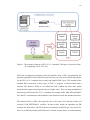
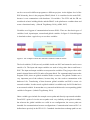


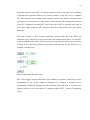

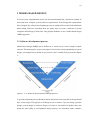


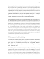
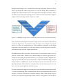
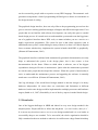


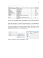

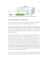

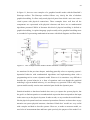
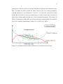
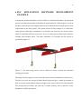

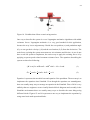
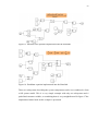
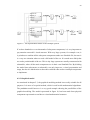
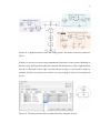

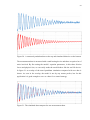
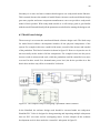
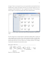
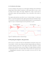

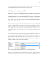
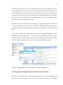
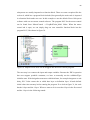

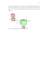

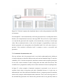
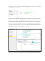

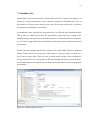

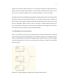
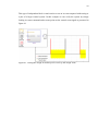
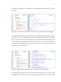
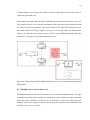


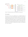
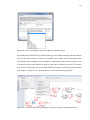


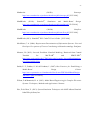



![CAST for PSI user`s manual [v07]](http://vs1.manualzilla.com/store/data/005903758_1-a858c2dfda3ffb28451a6ec48d1cfa02-150x150.png)