Download Using LaTeX to Write a PhD Thesis

Using LATEX to Write a PhD Thesis
Version 1.3
Nicola L. C. Talbot
Dickimaw Books
www.dickimaw-books.com
16th March, 2013
Copyright © 2007 Nicola L. C. Talbot
Permission is granted to copy, distribute and/or modify this document
under the terms of the GNU Free Documentation License, Version 1.2 or
any later version published by the Free Software Foundation; with no Invariant Sections, no Front-Cover Texts, and one Back-Cover Text: “If you
choose to buy a copy of this book, Dickimaw Books asks for your support
through buying the Dickimaw Books edition to help cover costs.” A copy
of the license is included in the section entitled “GNU Free Documentation
License”.
The base URL for this document is: http://www.dickimaw-books.com/
latex/thesis/
Contents
Abstract
1
vi
Introduction
1.1
1
Building Your Document . . . . . . . . . . . . . . . . . . . . . .
1.1.1 LaTeXmk . . . . . . . . . . . . . . . . . . . . . . . . . . . . .
1.1.2 Arara . . . . . . . . . . . . . . . . . . . . . . . . . . . . . . .
3
5
7
2
Getting Started
13
3
Splitting a Large Document into Several Files
17
4
Formatting
21
4.1
4.2
4.3
4.4
4.5
4.6
4.7
4.8
4.9
5
.
.
.
.
.
.
.
.
.
.
.
.
.
.
.
.
.
.
.
.
.
.
.
.
.
.
.
.
.
.
.
.
.
.
.
.
.
.
.
.
.
.
.
.
.
.
.
.
.
.
.
.
.
.
.
.
.
.
.
.
.
.
.
.
.
.
.
.
.
.
.
.
.
.
.
.
.
.
.
.
.
.
.
.
.
.
.
.
.
.
.
.
.
.
.
.
.
.
.
.
.
.
.
.
.
.
.
.
.
.
.
.
.
.
.
.
.
.
.
.
.
.
.
.
.
.
.
.
.
.
.
.
.
.
.
.
.
.
.
.
.
.
.
.
.
.
.
.
.
.
.
.
.
.
.
.
.
.
.
.
.
.
.
.
.
.
.
.
.
.
.
.
.
.
.
.
.
.
.
.
.
.
.
.
.
.
.
Generating a Bibliography
5.1
5.2
5.3
6
Changing the Document Style . .
Changing the Page Style . . . . .
Double-Spacing . . . . . . . . . . .
Changing the Title Page . . . . . .
Listings and Other Verbatim Text
Tabbing . . . . . . . . . . . . . . . .
Theorems . . . . . . . . . . . . . . .
4.7.1 The amsthm Package . . . . .
4.7.2 The ntheorem Package . . . .
Algorithms . . . . . . . . . . . . . .
Formatting SI Units . . . . . . . . .
Creating a Bibliography Database . .
5.1.1 JabRef . . . . . . . . . . . . . . . .
5.1.2 Writing the .bib File Manually .
BibTeX . . . . . . . . . . . . . . . . . . .
5.2.1 Author–Year Citations . . . . . .
5.2.2 Troubleshooting . . . . . . . . .
Biblatex . . . . . . . . . . . . . . . . . .
5.3.1 Troubleshooting . . . . . . . . .
46
.
.
.
.
.
.
.
.
.
.
.
.
.
.
.
.
.
.
.
.
.
.
.
.
.
.
.
.
.
.
.
.
Generating Indexes and Glossaries
6.1
6.2
21
21
23
24
25
30
32
34
38
41
44
.
.
.
.
.
.
.
.
.
.
.
.
.
.
.
.
.
.
.
.
.
.
.
.
.
.
.
.
.
.
.
.
.
.
.
.
.
.
.
.
.
.
.
.
.
.
.
.
.
.
.
.
.
.
.
.
.
.
.
.
.
.
.
.
.
.
.
.
.
.
.
.
.
.
.
.
.
.
.
.
.
.
.
.
.
.
.
.
46
47
59
62
64
65
66
72
73
Using an External Indexing Application . . . . . . . . . . . . . 73
6.1.1 Creating an Index (makeidx package) . . . . . . . . . . . . 74
6.1.2 Creating Glossaries, Lists of Symbols or Acronyms (glossaries
package) . . . . . . . . . . . . . . . . . . . . . . . . . . . . . 80
Using LATEX to Sort and Collate Indexes or Glossaries (datagidx
package) . . . . . . . . . . . . . . . . . . . . . . . . . . . . . . . . . 90
i
Contents
ii
A General Advice
A.1
A.2
99
Too Many Unprocessed Floats . . . . . . . . . . . . . . . . . . . 99
General Thesis Writing Advice . . . . . . . . . . . . . . . . . . . 100
Bibliography
103
Acronyms
105
Summary of Commands and Environments
106
Index
123
GNU Free Documentation License
129
History
137
List of Figures
1.1
1.2
1.3
1.4
1.5
1.6
1.7
1.8
1.9
Selecting pdfLaTeX from the Drop-Down Menu . . . . . . . . .
3
Selecting BibTeX from the Drop-Down Menu . . . . . . . . . .
4
Adding Makeglossaries to the list of tools in TeXworks . . . .
4
TeXwork’s Preferences Dialog Box . . . . . . . . . . . . . . . . .
6
Adding LaTeXmk in the TeXWorks Tool Configuration Dialog 6
LaTeXmk Tool Selected in TeXworks . . . . . . . . . . . . . . .
8
Arara Installer . . . . . . . . . . . . . . . . . . . . . . . . . . . . . .
9
Adding Arara in the TeXWorks Tool Configuration Dialog . . 10
Using Arara in TeXworks . . . . . . . . . . . . . . . . . . . . . . . 11
4.1
4.2
Page Header and Footer Elements . . . . . . . . . . . . . . . . .
Sample Title Page . . . . . . . . . . . . . . . . . . . . . . . . . . . .
22
26
5.1
5.2
5.3
5.4
5.5
5.6
5.7
5.8
5.9
5.10
5.11
5.12
5.13
5.14
5.15
5.16
5.17
JabRef . . . . . . . . . . . . . . . . . . . . . . . . . . . . . . . .
JabRef Preferences . . . . . . . . . . . . . . . . . . . . . . . .
JabRef Database Properties . . . . . . . . . . . . . . . . . . .
JabRef (Select Entry Type) . . . . . . . . . . . . . . . . . . .
JabRef (New Entry) . . . . . . . . . . . . . . . . . . . . . . . .
JabRef (Entering the Required Fields) . . . . . . . . . . . .
JabRef (Entering Optional Fields) . . . . . . . . . . . . . . .
JabRef (Adding an Article) . . . . . . . . . . . . . . . . . . . .
JabRef (Adding a Conference Paper) . . . . . . . . . . . . .
JabRef (Adding Editor List) . . . . . . . . . . . . . . . . . . .
Importing a Plain Text Reference . . . . . . . . . . . . . . .
Importing a Plain Text Reference (Selecting a Field) . . .
Importing a Plain Text Reference (Field Selected) . . . . .
JabRef Advanced Preferences . . . . . . . . . . . . . . . . .
JabRef in BibLaTeX Mode . . . . . . . . . . . . . . . . . . . .
JabRef in BibLaTeX Mode (Select Entry Type) . . . . . . .
JabRef in BibLaTeX Mode (Setting the Publication Date) .
48
48
49
49
50
51
52
53
55
56
57
58
58
67
67
68
69
.
.
.
.
.
.
.
.
.
.
.
.
.
.
.
.
.
.
.
.
.
.
.
.
.
.
.
.
.
.
.
.
.
.
.
.
.
.
.
.
.
.
.
.
.
.
.
.
.
.
.
iii
List of Tables
4.1
Theorem Styles . . . . . . . . . . . . . . . . . . . . . . . . . . . . .
39
5.1
5.2
5.3
5.4
Name Formats for Bibliographic Data
Standard BiBTeX entry types . . . . . .
Standard BiBTeX fields . . . . . . . . .
Required and Optional Fields . . . . . .
53
59
60
61
.
.
.
.
.
.
.
.
.
.
.
.
.
.
.
.
.
.
.
.
.
.
.
.
.
.
.
.
.
.
.
.
.
.
.
.
.
.
.
.
.
.
.
.
.
.
.
.
.
.
.
.
.
.
.
.
.
.
.
.
iv
Listings
1
2
3
4
5
6
7
8
9
10
11
12
13
14
15
16
17
18
19
20
21
Getting Started . . . . . . . . . . . . . . . . . . . . . . . . . . . . .
Splitting a Large Document into Several Files (thesis.tex) .
Splitting a Large Document into Several Files (intro.tex) .
Splitting a Large Document into Several Files (techintro.tex)
Splitting a Large Document into Several Files (method.tex) .
Splitting a Large Document into Several Files (results.tex)
Splitting a Large Document into Several Files (conc.tex) . .
Changing the Page Style . . . . . . . . . . . . . . . . . . . . . .
Double-Spacing . . . . . . . . . . . . . . . . . . . . . . . . . . . .
Changing the Title Page . . . . . . . . . . . . . . . . . . . . . . .
Listings and Other Verbatim Text . . . . . . . . . . . . . . . . .
The amsthm Package . . . . . . . . . . . . . . . . . . . . . . . . .
The ntheorem Package . . . . . . . . . . . . . . . . . . . . . . . . .
Algorithms . . . . . . . . . . . . . . . . . . . . . . . . . . . . . . .
BibTeX . . . . . . . . . . . . . . . . . . . . . . . . . . . . . . . . . .
Author–Year Citations . . . . . . . . . . . . . . . . . . . . . . . .
Biblatex . . . . . . . . . . . . . . . . . . . . . . . . . . . . . . . . .
Creating an Index (makeidx package) . . . . . . . . . . . . . . .
Creating an Index (makeidx package) . . . . . . . . . . . . . . .
Creating Glossaries, Lists of Symbols or Acronyms (glossaries
package) . . . . . . . . . . . . . . . . . . . . . . . . . . . . . . . . .
Using LATEX to Sort and Collate Indexes or Glossaries (datagidx
package) . . . . . . . . . . . . . . . . . . . . . . . . . . . . . . . . .
14
18
19
19
19
19
20
23
24
24
29
35
40
43
63
65
71
74
78
89
96
v
Abstract
This book is aimed at PhD students who want to use LATEX to typeset their
PhD thesis. If you are unfamiliar with LATEX I recommend that you first
read Volume 1: LATEX for Complete Novices [15].
vi
Chapter 1
Introduction
Many PhD students in the sciences are encouraged to produce their PhD
thesis in LATEX, particularly if their work involves a lot of mathematics. In
addition, these days, LATEX is no longer the sole province of mathematicians
and computer scientists and is now starting to be used in the arts and social sciences (see, for example, some of the topics listed in the TEX online
catalogue [3]). This book is intended as a brief guide on how to typeset
the various components that are usually required for a thesis. If you have
never used LATEX before, I recommend that you first read Volume 1: LATEX
for Complete Novices [15], as this book assumes you have a basic knowledge of LATEX. As with Volume 1, I’ll be using PDFLATEX and TeXWorks. If
you are creating a DVI file or you are using a different editor, you’ll have to
adapt the instructions.
B
If you are unfamiliar with terms such as “preamble”, read Volume 1 [15,
§2]. If you don’t know how to find package documentation, read Volume 1 [15,
§1.1].
Throughout this document there are pointers to related topics in the UK
List of TEX Frequently Asked Questions1.1 (UK FAQ). These are displayed
in the margin in square brackets, as illustrated on the right. You may find [FAQ: What is
these resources useful in answering related questions that are not covered LaTeX?]
in this book.
On-line versions of this book, along with associated files, are available at:
http://www.dickimaw-books.com/latex/thesis/. The links in this document are colour-coded: internal links are blue, external links are magenta.
To refresh your memory or for those who haven’t read Volume 1, throughout this book source code is illustrated in a typewriter font with the word
Input placed in the margin, and the corresponding output (how it will appear
in the PDF document) is typeset with the word Output in the margin.
Example:
A single line of code is displayed like this:
This is an \textbf{example}.
Input
The corresponding output is illustrated like this:
This is an example.
Output
Segments of code that are longer than one line are bounded above and
below, illustrated as follows:
1.1
http://www.tex.ac.uk/faq
1
Chapter 1 Introduction
2
↑ Input
Line one\par
Line two\par
Line three.
↓ Input
with corresponding output:
↑ Output
Line one
Line two
Line three.
↓ Output
(Commands typeset in blue, such as \par, indicate a hyperlink to the command definition in the summary.)
Command definitions are shown in a typewriter font in the form:
\documentclass[⟨options⟩]{⟨class file⟩}
Definition
In this case the command being defined is called \documentclass and text
typed ⟨like this⟩ (such as ⟨options⟩ and ⟨class file⟩) indicates the type of
thing you need to substitute. (Don’t type the angle brackets!) For example,
if you want the scrbook class file you would substitute ⟨class file⟩ with scrbook
and if you want the letterpaper option you would substitute ⟨options⟩ with
letterpaper, like this:
\documentclass[letterpaper]{scrbook}
Input
When it’s important to indicate a space, the visible space symbol ␣ is used.
For example:
A␣sentence␣consisting␣of␣six␣words.
Input
When you type up the code, replace any occurrences of ␣ with a space.
Note:
Be careful of the dangers of obsolete code propagation. It often happens
that students pass on their LATEX code to new students who, in their turn,
pass it on to the next lot of students, and so on. You’re told “use this magic bit
of code to format your thesis” without knowing what it does. Ancient buggy
code that’s 20 years out-of-date festers in university departments refusing to
die. But if it worked for previous students, what’s the problem? The problem
is that it may stop working a week before your submission date and when
you go for help, you may be told you’re using obsolete packages and there’s
nothing for it but to rewrite your thesis using the modern alternatives.
How do you know if a package is obsolete? Some of the obsolete packages and commands are listed in l2tabu [18], or you can check to see if
a package is listed in the Comprehensive TEX Archive Network1.2 (CTAN)’s
obsolete tree (http://mirror.ctan.org/obsolete/). Stefan Kottwitz also
has a list of obsolete classes and packages in his TeXblog. The other thing
1.2
http://mirror.ctan.org/
B
Chapter 1 Introduction
3
to do is check the package’s entry on CTAN [2] to see if it has been deprecated. For example, suppose someone tells you to use the glossary package.
If you go to http://ctan.org/pkg/glossary it will tell you that the glossary
package is no longer supported and that it’s been replaced by the glossaries
package. Similarly, if you go to http://ctan.org/pkg/epsfig it will tell you
that the epsfig package is obsolete and you should use graphicx instead.
1.1 Building Your Document
To “typeset”, “build”, “compile” or “LaTeX” your document means to run the
pdflatex (or latex) executable on your document source code. If you are
using a front-end, such as TeXworks, WinEdt, TeXstudio, or TeXnicCenter,
this usually just means clicking on the appropriate button or selecting the
appropriate menu item. (See Volume 1 [15, §3] for further details.)
It’s important to remember that a front-end is an interface. It’s not,
for example, TeXworks that is creating your PDF. When you click on the
“typeset” button, TeXworks tells the operating system to run the required
executable. This is usually pdflatex, but there are other executables that
may need to be used to help create your document, such as bibtex or
biber (discussed in Chapter 5 (Generating a Bibliography)) and makeindex
or xindy (discussed in Chapter 6 (Generating Indexes and Glossaries)).
For example, if your document has a bibliography and you are using
TeXworks, you first need to make sure the drop-down menu is set to “pdfLaTeX” (see Figure 1.1) and click on the green “Typeset” button. Then you need
to select “BibTeX” from the drop-down menu (see Figure 1.2) and click on
the green “Typeset” button. Then again select “pdfLaTeX” (Figure 1.1) and
click the “Typeset” button. Finally, to ensure your cross-references are all
up-to-date, you need to click on the “Typeset” button again. If you are using
biber instead of bibtex (see Section 5.3), then you have to replace the above
“BibTeX” step with “Biber” instead.
Figure 1.1 Selecting pdfLaTeX from the Drop-Down Menu
Chapter 1 Introduction
4
Figure 1.2 Selecting BibTeX from the Drop-Down Menu
If the tool you require isn’t listed in the drop-down box, you will have
to add it. For example, to add makeglossaries to the list of available tools
in TeXworks, you need to select EditÏPreferences, which will open the “TeXworks Preferences” dialog. Make sure the “Typesetting” tab is selected and
click on the lower button next to the “Processing tools” list. This will open
the “Tool Configuration” dialog. Set the “Name” field to the name of the
application, as you want it to appear in the tool list (for example “MakeGlossaries”). Then click on the “Browse” button to find the application on your
button next to the “Arguments”
computer. Next you need to click on the
list. Set the argument to $basename. Since makeglossaries doesn’t modify
the PDF, uncheck the “View PDF after running” box (see Figure 1.3).
Figure 1.3 Adding Makeglossaries to the list of tools in TeXworks
This is a bit of a hassle (if not downright confusing for a beginner) and
Chapter 1 Introduction
5
even more so when you have glossaries and an index in your document
as well as a bibliography. Fortunately there are ways of automating this
process so that you only need one button press to perform all those different steps. There are several applications available to do this for you,
and I strongly recommend you try one of them, if possible, to reduce the
complexity involved in building a document.
Volume 1 [15, §5.5] mentioned latexmk, which is available on CTAN [2].
This is a Perl script, so it will run on any operating system that has Perl
installed (see Volume 1 [15, §2.20]). Since Volume 1 was published, a Java
alternative called arara has arrived on CTAN [2]. Java applications will run
on any operating system that has the Java Runtime Environment installed,
so both latexmk and arara are multi-platform solutions to automated document compilation. Section 1.1.1 gives a brief introduction to latexmk, and
Section 1.1.2 gives a brief introduction to arara.
1.1.1 LaTeXmk
As mentioned above, latexmk is a Perl script that automates the process of
building a LATEX document. In order to use latexmk, you must have Perl
installed (see Volume 1 [15, §2.20]). Both TeX Live and MikTeX come with
latexmk but, if for some reason you don’t have it installed, you can use
the TeX Live or MikTeX update manager to install it. Alternatively, you
can download http://mirror.ctan.org/support/latexmk.zip and install it
manually.
Once latexmk is installed, you then need to add it to the list of available
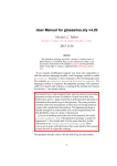
tools in TeXworks1.3 . This is done via the EditÏPreferences menu item. This
opens TeXwork’s Preferences dialog box. Make sure the “Typesetting” tab
is selected (Figure 1.4).
button next to the list of proTo add a new tool, click on the lower
cessing tools. This opens the tool configuration dialog box (Figure 1.5).
Type “LaTeXmk” in the “Name” box, then use the “Browse” button to
button
locate latexmk on your computer. Next you need to click on the
to add each argument. The argument list should consist of the following (in
the order listed):
-e
$pdflatex=q/pdflatex $synctexoption %O %S/
-pdf
-bibtex
$fullname
Once you’ve done this, click “Okay” to close the tool configuration dialog,
and click “Okay” to close the Preferences dialog box. LaTeXmk should now
be listed in the drop-down menu next to the green “Typeset” button. Now, if
you have LaTeXmk selected and you click on the “Typeset” button pdflatex
and bibtex/biber will be run as necessary to create an up-to-date PDF.
1.3
If you are using a different front-end, you will have to consult your front-end’s manual.
Chapter 1 Introduction
6
Figure 1.4 TeXwork’s Preferences Dialog Box
Figure 1.5 Adding LaTeXmk in the TeXWorks Tool Configuration Dialog
Chapter 1 Introduction
7
Unfortunately, adding makeindex, texindy or makeglossaries to LaTeXmk’s
set of rules is more complicated. For this you need to create a configuration/initialisation (RC) file1.4 . The name and location of this file depends on
your operating system. For example, on a Unix-like operating system, this
may be $HOME/.latexmkrc. You will need to consult the latexmk manual [1]
for further details.
Once you’ve found out the name and location of the RC file for your
operating system, you can use the text editor of your choice to create this
file. To add makeglossaries, you need to type the following in the RC file:
add_cus_dep(’glo’, ’gls’, 0, ’makeglossaries’);
add_cus_dep(’acn’, ’acr’, 0, ’makeglossaries’);
sub makeglossaries{
system( "makeglossaries \"$_[0]\"" );
}
To add makeindex, you need to type the following:
add_cus_dep(’idx’, ’ind’, 0, ’makeindex’);
sub makeindex{
system("makeindex \"$_[0].idx\"");
}
If you prefer to use texindy instead of makeindex, you will need to replace the above lines with (change the language as appropriate):
add_cus_dep(’idx’, ’ind’, 0, ’texindy’);
sub texindy{
system("texindy -L english \"$_[0].idx\"");
}
Now select “LaTeXmk” from the drop-down menu next to the green
“Typeset” button in TeXworks (Figure 1.6), and you’re ready to build your
documents.
1.1.2 Arara
As mentioned in Section 1.1, arara is a Java application that automates the
process of building a LATEX document. In order to use arara, you must have
the Java Runtime Environment installed. The latest TeX Live distribution
includes arara, so you can install it via the TeX Live package manager.
Alternative, you can install arara manually as follows: fetch the installer
arara-3.0-installer.jar (or arara-3.0-installer.exe) from https://
github.com/cereda/arara/tree/master/releases.
On Windows, run
arara-3.0-installer.exe.
On other operating systems run
arara-3.0-installer.jar in privileged mode. For example, on a Unixbased system:
sudo java -jar arara-3.0-installer.jar
Chapter 1 Introduction
Figure 1.6 LaTeXmk Tool Selected in TeXworks
8
Chapter 1 Introduction
9
Figure 1.7 Arara Installer
(If you are doing a manual install make sure you check the box to add the
predefined rules, as shown in Figure 1.7.)
Once arara has been installed, you can add it to the list of tools in TeXworks. As before, open the TeXwork’s Preferences dialog box using EditÏ
Preferences and select the “Typesetting” tab (Figure 1.4).
To add a new tool, click on the lower button next to the list of processing tools. This opens the tool configuration dialog box (Figure 1.8). Type
“Arara” in the “Name” box and use the “Browse” button to find the arara
button to add $basename to the
application on your computer. Use the
list of arguments, as shown in Figure 1.8.
Unlike latexmk, arara doesn’t read the log file to determine what applications need to be run. Instead, you tell arara how to build your document
by placing special comments in your source code. For example, if your
document contains the following:
↑ Input
% arara: pdflatex: { synctex: on }
% arara: bibtex
% arara: pdflatex: { synctex: on }
% arara: pdflatex: { synctex: on }
\documentclass{scrbook}
↓ Input
1.4
There are some example RC files available at: http://mirror.ctan.org/support/
latexmk/example_rcfiles/.
Chapter 1 Introduction
10
Figure 1.8 Adding Arara in the TeXWorks Tool Configuration Dialog
Then running arara on the document will run pdflatex, bibtex, pdflatex
and pdflatex on your document. Arara knows the rules “pdflatex” and
“bibtex”. It also knows the rules “biber”, “makeglossaries” and “makeindex”.
So, if your document has a bibliography, an index and glossaries, you need
to put the following comments in your source code (replace bibtex with
biber if required):
% arara: pdflatex: { synctex: on }
% arara: bibtex
% arara: makeglossaries
% arara: makeindex
% arara: pdflatex: { synctex: on }
% arara: pdflatex: { synctex: on }
\documentclass{scrbook}
↑ Input
↓ Input
Now you just need to select “Arara” from the drop-down list in TeXworks
(Figure 1.9) and click the green “Typeset” button, and arara will do all the
work for you.
Note:
If you don’t add these arara comments to your source code, nothing will
happen when you run arara on your document! You must remember to
provide arara with the rules to build your document.
Unfortunately arara (v3.0) doesn’t have a rule for texindy, but you can
add one by creating a file called texindy.yaml that contains the following:1.5
!config
# TeXindy rule for arara
1.5
Thanks to Paulo Cereda for supply this.
B
Chapter 1 Introduction
Figure 1.9 Using Arara in TeXworks
11
Chapter 1 Introduction
12
# requires arara 3.0+
identifier: texindy
name: TeXindy
command: <arara> texindy @{german} @{language} @{codepage} @{module}
Î˒
@{input} @{options} "@{getBasename(file)}.idx"
arguments:
- identifier: german
flag: <arara> @{isTrue(parameters.german,"-g")}
- identifier: language
flag: <arara> -L @{parameters.language}
- identifier: codepage
flag: <arara> -C @{parameters.codepage}
- identifier: module
flag: <arara> -M @{parameters.module}
- identifier: input
flag: <arara> -I @{parameters.input}
- identifier: options
flag: <arara> @{parameters.options}
(The symbol Î˒ above indicates a line wrap. Don’t insert a line break at that
point.) This file should be saved in the rules subdirectory of the arara installation directory. (For example, on Unix-like systems /usr/local/arara/
rules/texindy.yaml.)
So if you’d rather use texindy instead of makeindex you can replace the
% arara: makeindex
directive with
% arara: texindy: { language: english, codepage: latin1 }
(Change the language and encoding as appropriate.)
Chapter 2
Getting Started
There are many different thesis designs, varying according to university or
discipline [5]. If you have been told to use a particular class file, use that
one. If not, there are a selection of thesis class files available on CTAN [2]
and listed in the OnLine TEX Catalogue’s Topic Index [3]. Since there are
so many to choose from, I’m just going to follow on from Volume 1 of
this series and use one of the KOMA-Script class files. But which one?
The scrreprt class is the one usually recommended for a report or thesis. It
defaults to one-sided and has an abstract environment, but it doesn’t define
\frontmatter, \mainmatter or \backmatter. The scrbook class does define
those commands, but it doesn’t provide an abstract environment and defaults
to two-sided layout. So, you can either do:
↑ Input
\documentclass{scrreprt}
\title{A Sample Thesis}
\author{A.N. Other}
\begin{document}
\maketitle
\pagenumbering{roman}
\tableofcontents
\chapter*{Acknowledgements}
\begin{abstract}
This is the abstract
\end{abstract}
\pagenumbering{arabic}
\chapter{Introduction}
...
\end{document}
↓ Input
or you can do:
13
Chapter 2 Getting Started
14
↑ Input
\documentclass[oneside]{scrbook}
\title{A Sample Thesis}
\author{A.N. Other}
\begin{document}
\maketitle
\frontmatter
\tableofcontents
\chapter{Acknowledgements}
\chapter{Abstract}
This is the abstract
\mainmatter
\chapter{Introduction}
...
\end{document}
↓ Input
I’m going to use the second approach simply out of personal preference.
The KOMA-Script options mentioned in this book are available for both
scrreprt and scrbook, so choose whichever class file you feel best suits your
thesis.
Unless you have been told otherwise, I recommend that you start out
with a skeletal document that looks something like the following:
Listing 1
↑ Input
\documentclass[oneside]{scrbook}
\title{A Sample Thesis}
\author{A.N. Other}
\date{July 2013}
\titlehead{A Thesis submitted for the degree of Doctor of Philosophy}
\publishers{School of Something\\University of Somewhere}
\begin{document}
\maketitle
\frontmatter
\tableofcontents
\listoffigures
\listoftables
Chapter 2 Getting Started
15
\chapter{Acknowledgements}
I would like to thank my supervisor, Professor Someone. This
research was funded by the Imaginary Research Council.
\chapter{Abstract}
A brief summary of the project goes here.
% A glossary and list of acronyms may go here
% or may go in the back matter.
\mainmatter
\chapter{Introduction}
\label{ch:intro}
\chapter{Technical Introduction}
\label{ch:techintro}
\chapter{Method}
\label{ch:method}
\chapter{Results}
\label{ch:results}
\chapter{Conclusions}
\label{ch:conc}
\backmatter
% A glossary and list of acronyms may go here
% or may go in the front matter after the abstract.
% The bibliography will go here
\end{document}
↓ Input
If you do this, it will help ensure that your document has the correct
structure before you begin with the actual contents of the document. (Note
that the chapter titles will naturally vary depending on your subject or institution, and you may need a different paper size if you are not in Europe.
I have based the above on my own PhD thesis which I wrote in the early
to mid 1990s in the Department of Electronic Systems Engineering at the
University of Essex, and it may well not fit your own requirements.)
If you haven’t started your thesis yet, go ahead and try this. Creating
a skeletal document can have an amazing psychological effect on some
people: for very little effort it can produce a document several pages long,
Chapter 2 Getting Started
16
which can give you a sense of achievement that can help give you sufficient
momentum to get started (but of course, it’s not guaranteed to work with
everyone). Remember that if you want to use arara (see Section 1.1.2) you
must add the build rules to the document:
↑ Input
% arara: pdflatex: { synctex: on }
% arara: pdflatex: { synctex: on }
\documentclass[oneside]{scrbook}
↓ Input
(I’ll add the arara rules to sample listings, in the event that you want to use
arara. Since they are comments, they will be ignored if you use pdflatex
explicitly or if you use another automation method, such as latexmk.)
Now think about other requirements. What font size have you been told
to use?
10pt Use the 10pt class option:
\documentclass[oneside,10pt]{scrbook}
Input
11pt Use the 11pt class option:
\documentclass[oneside,11pt]{scrbook}
Input
12pt Use the 12pt class option:
\documentclass[oneside,12pt]{scrbook}
Input
Have you been told to have a blank line between paragraphs and no paragraph indentation? If so, use the parskip=full class option:
\documentclass[oneside,12pt,parskip=full]{scrbook}
Input
Have you been told to have certain sized margins? If so, you can use the [FAQ: Changing
geometry package. For example, if you have been told you must have 1 inch the margins in
LATEX]
margins, you can do
\usepackage[margin=1in]{geometry}
Changing the default fonts is covered in Volume 1 [15, §4.5.3]. Other possible
formatting requirements, such as double-spacing, are covered in Chapter 4
(Formatting).
Input
Chapter 3
Splitting a Large Document
into Several Files
Some people prefer to place each chapter of a large document in a separate
file and then input the file into the main document.
There are two basic ways of including the contents of an external file:
\input{⟨filename⟩}
Definition
and
\include{⟨filename⟩}
Definition
where ⟨filename⟩ is the name of the file. (The .tex extension may be
omitted in both cases.) The differences between the two commands are as
follows:
\input acts as though the contents of the file were typed where the \input
command was. For example, suppose my main file contained the following:
↑ Input
Here is a short paragraph.
\input{myfile}
↓ Input
and suppose the file myfile.tex contained the following lines:
↑ Input
Here is some sample text.
↓ Input
then the \input command behaves as though you had simply typed
the following in your main document file:
↑ Input
17
Chapter 3 Splitting a Large Document into Several Files
18
Here is a short paragraph.
Here is some sample text.
↓ Input
\include does more than just input the contents of the file. It also starts
a new page (using \clearpage) and creates an auxiliary file associated
with the included file. It also issues another \clearpage once the file
has been read in. Using this approach, you can also govern which files
to include using
\includeonly{⟨file list⟩}
Definition
in the preamble, where ⟨file list⟩ is a comma-separated list of files
you want included. This way, if you only want to work on one or two
chapters, you can only include those chapters, which will speed up
the document build. LATEX will still read in all the cross-referencing
information for the missing chapters, but won’t include those chapters
in the PDF file. There is a definite advantage to this if you have, say,
a large number of images in your results chapter, which you don’t need
when you’re working on, say, the technical introduction. You can still
reference all the figures in the omitted chapter, as long as you have
previously LATEXed the document without the \includeonly command.
The excludeonly package provides the logically opposite command:
\excludeonly{⟨file list⟩}
Definition
The previous example can now be split into various files:
Listing 2 (thesis.tex)
↑ Input
% arara: pdflatex: { synctex: on }
% arara: pdflatex: { synctex: on }
\documentclass[oneside]{scrbook}
\title{A Sample Thesis}
\author{A.N. Other}
\date{July 2013}
\titlehead{A Thesis submitted for the degree of Doctor of Philosophy}
\publishers{School of Something\\University of Somewhere}
\begin{document}
\maketitle
\frontmatter
\tableofcontents
\listoffigures
Chapter 3 Splitting a Large Document into Several Files
19
\listoftables
\chapter{Acknowledgements}
I would like to thank my supervisor, Professor Someone. This
research was funded by the Imaginary Research Council.
\chapter{Abstract}
A brief summary of the project goes here.
\mainmatter
\include{intro}
\include{techintro}
\include{method}
\include{results}
\include{conc}
\backmatter
\end{document}
↓ Input
Listing 3 (intro.tex)
↑ Input
\chapter{Introduction}
\label{ch:intro}
↓ Input
Listing 4 (techintro.tex)
↑ Input
\chapter{Technical Introduction}
\label{ch:techintro}
↓ Input
Listing 5 (method.tex)
↑ Input
\chapter{Method}
\label{ch:method}
↓ Input
Listing 6 (results.tex)
↑ Input
\chapter{Results}
\label{ch:results}
↓ Input
Chapter 3 Splitting a Large Document into Several Files
20
Listing 7 (conc.tex)
↑ Input
\chapter{Conclusions}
\label{ch:conc}
↓ Input
If you only want to work on, say, the Method and Results chapters, you
can place the following command in the preamble:
\includeonly{method,results}
Input
Chapter 4
Formatting
It used to be that in order to change the format of chapter and section
headings, you needed to have some understanding of the internal workings
of classes such as report or book. Modern classes, such as memoir and the
KOMA-Script classes, provide a much easier interface. However, I recommend that you first write your thesis, and then worry about changing the
document style. The ability to separate content from style is one of the advantages of using LATEX over a word processor. Remember that writing your
thesis is more important than the layout. Whilst it may be that your school
or department insists on a certain style, it should not take precedence over
the actual task of writing.
4.1 Changing the Document Style
If you are using a custom thesis class file provided by your department or
school, then you should stick to the styles set up in that class. If not, you may
need to change the default style of your chosen class to fit the requirements.
Volume 1 [15, §5.3] described how to change the fonts used by chapter and
section headings for the KOMA-Script classes. For example, if the chapter
headings must be set in a large, bold, serif font you can do:
\addtokomafont{\large\bfseries\rmfamily}
Input
The headings in the KOMA-Script classes default to ragged-right justification
(recall \raggedright from §2.12 of Volume 1) which is done via
\raggedsection
Definition
This can be redefined as required. For example, suppose you are required
to have centred headings, then you can do:
\renewcommand*{\raggedsection}{\centering}
Input
4.2 Changing the Page Style
Volume 1 [15, §5.7] described the command
\pagestyle{⟨style⟩}
Definition
which can be used to set the page style. The scrbook class defaults to the
headings page style, but if this isn’t appropriate, you can use the scrpage2
21
Chapter 4 Formatting
22
package, which comes with the KOMA-Script bundle. This package provides its own versions of the plain and headings page styles, called scrplain
and scrheadings.
For simplicity, I’m assuming that your thesis is a one-sided document. If
this isn’t the case and your odd and even page styles need to be different,
you’ll need to consult the KOMA-Script documentation [8].
With the scrheadings page style, the page header and footer are both
divided into three areas (Figure 4.1): the inner (left) head/foot, the centre
head/foot and the outer (right) head/foot.
ihead
chead
ohead
ifoot
cfoot
ofoot
Figure 4.1 Page Header and Footer Elements
These elements can be set using:
\ihead[⟨scrplain
\chead[⟨scrplain
\ohead[⟨scrplain
\ifoot[⟨scrplain
\cfoot[⟨scrplain
\ofoot[⟨scrplain
inner head⟩]{⟨scrheadings inner head⟩}
centre head⟩]{⟨scrheadings centre head⟩}
outer head⟩]{⟨scrheadings outer head⟩}
inner foot⟩]{⟨scrheadings inner foot⟩}
centre foot⟩]{⟨scrheadings centre foot⟩}
outer foot⟩]{⟨scrheadings outer foot⟩}
In each case, the optional argument indicates what to do if the scrplain
page style is in use and the mandatory argument indicates what to do if the
scrheadings page style is in use. (If the optional argument is missing, no
Definition
Chapter 4 Formatting
23
modification is made to the scrplain style.) Within both types of argument,
you can use
\pagemark
Definition
to insert the current page number and
\headmark
Definition
to insert the running heading. For example, suppose you are required to
put your registration number on the bottom left of each page and the page
number on the bottom right, and you are also required to put the current
chapter or section heading at the top left of each page, unless it’s the first
page of a chapter. Then you can do:
Listing 8
↑ Input
\usepackage{scrpage2}
\pagestyle{scrheadings}
\newcommand{\myregnum}{123456789}% registration number
\ihead{}
\chead{}
\ohead[]{\headmark}
\ifoot[\myregnum]{\myregnum}% registration number
\cfoot[]{}
\ofoot[\pagemark]{\pagemark}
↓ Input
Note that the above don’t use any font changing commands. If you
want to change the font for the header and footer, you need to redefine
\headfont. The page number style is given by \pnumfont. So for italic
headers and footers with bold page numbers, you can redefine these commands as follows:
\renewcommand*{\headfont}{\normalfont\itshape}
\renewcommand*{\pnumfont}{\normalfont\bfseries}
4.3 Double-Spacing
Whilst double-spacing is usually frowned upon in the world of modern typesetting, it is usually a requirement for anything that may need hand-written
annotations, which can include theses. This extra space gives the examiners
room to write comments.4.1
4.1
Despite the current digital age, many people still use hand-written annotations on
manuscripts. It’s unlikely that your examiners have pens that are incompatible with
your paper.
↑ Input
↓ Input
Chapter 4 Formatting
24
Double-spacing can be achieved via the setspace package. You can either
set the spacing using the package options singlespacing, onehalfspacing
or doublespacing, or you can switch via the declarations:
\singlespacing
\onehalfspacing
\doublespacing
Definition
So, if your thesis has to be double-spaced, you can do:
Listing 9
↑ Input
\usepackage[doublespacing]{setspace}
↓ Input
4.4 Changing the Title Page
Volume 1 [15, §5.1] described how to lay out the title page using \maketitle.
If this layout isn’t appropriate for your school or department’s specifications,
you can lay out the title page manually using the titlepage environment instead
of \maketitle. Within this environment, you can use \hspace{⟨length⟩} and
\vspace{⟨length⟩} to insert horizontal and vertical spacing. (The unstarred
versions are ignored if they occur at the start of a line or page, respectively.
The starred versions will insert the given spacing, regardless of their location.) You can also use \hfill and \vfill, which will expand to fill the
available space horizontally or vertically, respectively.
Example:
Listing 10
\begin{titlepage}
\centering
\vspace*{1in}
\begin{Large}\bfseries
A Sample PhD Thesis\par
\end{Large}
\vspace{1.5in}
\begin{large}\bfseries
A. N. Other\par
\end{large}
\vfill
A Thesis submitted for the degree of Doctor of Philosophy
\par
\vspace{0.5in}
School of Something
\par
University of Somewhere
\par
\vspace{0.5in}
↑ Input
Chapter 4 Formatting
25
July 2013
\par
\end{titlepage}
↓ Input
The result is shown in Figure 4.2. (If you require double-spacing, you may
need to wait until after the title page before switching to double-spacing.)
4.5 Listings and Other Verbatim Text
[FAQ: Code
There may be times when you want to include text exactly as you have listings in LATEX]
typed it into your source code. For example, you may want to include
a short segment of computer code. This can be done using the verbatim
environment.
Example:
Note how I don’t need to worry about special characters, such as #, within
the verbatim environment:
↑ Input
\begin{verbatim}
#include <stdio.h> /* needed for printf */
int main()
{
printf("Hello World\n");
return 1;
}
\end{verbatim}
↓ Input
This just produces:
↑ Output
#include <stdio.h> /* needed for printf */
int main()
{
printf("Hello World\n");
return 1;
}
↓ Output
A more sophisticated approach is to use the listings package. With this
package, you first need to specify the programming language. For example,
the above code is in C, so I need to specify this using:
\lstset{language=C}
Now I can use the lstlisting environment to typeset my C code:
Input
Chapter 4 Formatting
26
A Sample PhD Thesis
A. N. Other
A Thesis submitted for the degree of Doctor of Philosophy
School of Something
University of Somewhere
July 2013
Figure 4.2 Sample Title Page
Chapter 4 Formatting
27
↑ Input
\begin{lstlisting}
#include <stdio.h> /* needed for printf */
int main()
{
printf("Hello World\n");
return 1;
}
\end{lstlisting}
↓ Input
The resulting output looks like:
#include <s t d i o . h> / ∗ needed f o r p r i n t f ∗ /
↑ Output
i n t main ( )
{
p r i n t f ( " Hello World\n " ) ;
return 1 ;
}
↓ Output
I can also have inline code snippets using:
\lstinline[⟨options⟩]⟨char⟩⟨code⟩⟨char⟩
Definition
This is different syntax to the usual forms of command argument. You can
chose any character ⟨char⟩ that isn’t the open square bracket [ and that
doesn’t occur in ⟨code⟩ to delimit the code, but the start and end ⟨char⟩
must match. (The optional argument is discussed below.) So the following
are all equivalent:
1. ⟨char⟩ is the exclamation mark character:
\lstinline!#include <stdio.h>!
Input
2. ⟨char⟩ is the vertical bar character:
\lstinline|#include <stdio.h>|
Input
3. ⟨char⟩ is the double-quote character:
\lstinline"#include <stdio.h>"
Input
4. ⟨char⟩ is the plus symbol:
\lstinline+#include <stdio.h>+
And so on, but ⟨char⟩ can’t be, say, # as that occurs in ⟨code⟩. Example:
Input
Chapter 4 Formatting
28
The stdio header file (required for the \lstinline+printf+
function) is loaded using the directive \lstinline!#include
<stdio.h>! on the first line.
↑ Input
↓ Input
Result:
↑ Output
The stdio header file (required for the printf function) is loaded using
the directive #include <stdio.h> on the first line.
Another alternative is to input the code from an external file. For example, suppose my C code is contained in the file helloworld.c, then I can
input it using:
\lstinputlisting[⟨options⟩]{helloworld.c}
(Remember to use a forward slash / as the directory divider, even if you
are using Windows.)
All the above (\lstinline, \lstinputlisting and the lstlisting environment) have an optional argument ⟨options⟩ that can be used to override
the default settings. These are ⟨key⟩=⟨value⟩ options. There are a lot of
options available, but I’m only going to cover a few. If you want more detail,
have a look at the listings documentation [6].
↓ Output
Input
title={⟨text⟩} is used to set an unnumbered and unlabelled title. If ⟨text⟩
contains a comma or equal sign, make sure you enclose ⟨text⟩ in curly
braces { and }.
caption={[⟨short⟩]⟨text⟩} is used to set a numbered caption. The optional
part ⟨short⟩ is an alternative short caption for the list of listings, which
can be produced using
\lstlistoflistings
As above, if the caption contains a comma or equal sign, make sure
you enclose it in curly braces { and }.
label={⟨text⟩} is used to assign a label to this listing so the number can be
referenced via \ref.
numbers={⟨setting⟩} The value ⟨setting⟩ may be one of: none (no line numbers), left (line numbers on the left) or right (line numbers on the
right).
mathescape This is a boolean key that can either be true (dollar $ character acts as the usual math mode shift) or false (deactivates the usual
behaviour of $).
basicstyle={⟨declaration⟩} The value (one or more declarations) is used
at the start of the listing to set the basic font style. For example,
⟨declaration⟩ could be \ttfamily (which actually makes more sense
for a listing).
Definition
Chapter 4 Formatting
29
Note:
If you set basicstyle to \ttfamily and you want bold keywords, make sure
you are using a typewriter font that supports bold, as not all of them do.
(Recall from Volume 1 [15, §4.5.3] how to change the font family.) This book
uses txtt (see Volume 1 [15, §8.2]). Other possibilities include beramono, tgcursor, courier, DejaVuSansMono (or dejavu to load the serif and sans-serif DejaVu
fonts as well), lmodern and luximono.
B
KOMA and listings
If you want to use the listings package with one of the KOMA-Script classes,
you need to load scrhack before listings, otherwise you will get a warning that
looks like:
B
Class scrbook Warning: Usage of deprecated \float@listhead!
(scrbook)
You should use the features of package ‘tocbasic’
(scrbook)
instead of \float@listhead.
(scrbook)
Definition of \float@listhead my be removed from
(scrbook)
‘scrbook’ soon, so it should not be used on input
line 57.
Example:
Listing 11
↑ Input
\begin{lstlisting}[language=C,basicstyle=\ttfamily,
mathescape=true]
#include <stdio.h> /* needed for printf */
#include <math.h> /* needed for sqrt */
int main()
{
double x = sqrt(2.0); /* $x = \sqrt{2}$ */
printf("x = %f\n", x);
return 1;
}
\end{lstlisting}
↓ Input
Result:
↑ Output
# include <stdio.h> /* needed for printf */
# include <math.h> /* needed for sqrt */
int main ()
{
√
double x = sqrt (2.0); /* 𝑥 = 2 */
Chapter 4 Formatting
30
printf ("x␣=␣%f\n", x);
return 1;
}
↓ Output
If you are using double-spacing, you may need to temporarily switch it off
in the listings. You can do this by adding \singlespacing to the basicstyle
setting.
\lstset{basicstyle={\ttfamily\singlespacing}}
Input
(Check with your supervisor to find out if listings should be double- or
single-spaced.)
Note:
It is not usually appropriate to have reams of listings in your thesis. It can
annoy an examiner if you have included every single piece of code you
have written during your PhD, as it comes across as padding to make it
look as though your thesis is a lot larger than it really is. (Examiners are
not easily fooled, and it’s best not to irritate them as it is likely to make them
less sympathetic towards you.) If you want to include listings in your thesis,
check with your supervisor first to find out whether or not it is appropriate. B
Be careful when you use verbatim-like environments or commands, such
as verbatim, lstlisting, \lstinline and \lstinputlisting. In general, they can’t
be used in the argument of another command.
[FAQ: Why
4.6 Tabbing
doesn’t verbatim
work within . . . ?]
The tabbing environment lets you create tab stops so that you can tab to
a particular distance from the left margin. Within the tabbing environment,
you can use the command \= to set a tab stop, \> to jump to the next tab
stop, \< to go back a tab stop, \+ to shift the left border by one tab stop to
the right, \- to shift the left border by one tab stop to the left. In addition,
\\ will start a new line and \kill will set any tabs stops defined in that line,
but will not typeset the line itself.
Note:
B
You may recall two of the above commands from Volume 1: \- was described as a discretionary hyphen in §2.14 and \= was described as the
macron accent command in §4.3. These two commands take on different meanings when they are used in the tabbing environment. If you want [FAQ: Accents
accents in your tabbing environment, either use the inputenc package (see misbehave in
Volume 1 [15, §4.3.1]) or use \a⟨accent symbol⟩{⟨c⟩}, for example \a"{u} tabbing]
instead of \"{u}.
Chapter 4 Formatting
31
Example:
↑ Input
\begin{tabbing}
Zero \=One \=Two \=Three\\
\>First tab stop\\
\>A\>\>B\\
\>\>Second tab stop
\end{tabbing}
↓ Input
This produces the following output:
↑ Output
Zero One Two Three
First tab stop
A
B
Second tab stop
↓ Output
Another Example:
This example sets up four tab stops, but ignores the first line:
↑ Input
\begin{tabbing}
AAA \=BBBB \=XX \=YYYYYY \=Z \kill
\>\>\>Third tab stop\\
\>a \>b \> \>c
\end{tabbing}
↓ Input
This produces the following output:
↑ Output
a
b
Third tab stop
c
↓ Output
Chapter 4 Formatting
32
4.7 Theorems
A PhD thesis can often contain theorems, lemmas, definitions etc. The LATEX
kernel comes with the command:
\newtheorem{⟨name⟩}[⟨counter⟩]{⟨title⟩}[⟨outer counter⟩]
Definition
which can be used to create an environment called ⟨name⟩ that has an
optional argument. Each instance of the environment starts with ⟨title⟩
followed by the associated counter value. If ⟨counter⟩ is present, the new
environment uses that counter instead of having a new counter defined for
it. If ⟨outer counter⟩ is present, the environment counter is reset every
time ⟨outer counter⟩ is incremented. The optional arguments are mutually
exclusive.
In the example below, I’ve use \newtheorem to define a new environment
called theorem, which has an associated counter, also called theorem, that is
dependant on the chapter counter.
↑ Input
% in the preamble:
\newtheorem{theorem}{Theorem}[chapter]
% later in the document:
\begin{theorem}
If proposition $P$ is a tautology
then $\sim P$ is a contradiction,
and conversely.
\end{theorem}
↓ Input
Resulting output:
Theorem 4.1 If proposition 𝑃 is a tautology then ∼ 𝑃 is a contradiction,
and conversely.
↑ Output
↓ Output
The optional argument to the new environment can be used to add a caption.
Modifying the above example (changes shown like this):
↑ Input
% in the preamble:
\newtheorem{theorem}{Theorem}[chapter]
% later in the document:
\begin{theorem}[Tautologies and Contradictions]
If proposition $P$ is a tautology
then $\sim P$ is a contradiction,
and conversely.
\end{theorem}
↓ Input
Chapter 4 Formatting
33
Resulting output:
↑ Output
Theorem 4.2 (Tautologies and Contradictions) If proposition 𝑃 is a tautology then ∼ 𝑃 is a contradiction, and conversely.
↓ Output
Here’s an example that uses the first optional argument of \newtheorem:
↑ Input
% in the preamble:
\newtheorem{exercise}{Exercise}
\newtheorem{suppexercise}[exercise]{Supplementary Exercise}
% later in the document:
\begin{exercise}
This is an example of how to create a theorem-like environment.
\end{exercise}
\begin{suppexercise}
This is another example of how to create a theorem-like environment.
\end{suppexercise}
↓ Input
Result:
↑ Output
Exercise 1 This is an example of how to create a theorem-like environment.
Supplementary Exercise 2 This is another example of how to create a
theorem-like environment.
↓ Output
Unfortunately there isn’t a great deal of flexibility with the environment
appearance. However there are various packages available that provide en- [FAQ: Theorem
hancements to this basic command, allowing you to adjust the appearance bodies printed in
to suit your requirements. There seem to be two main contenders: amsthm a roman font]
and ntheorem. Both have advantages and disadvantages. For example, ntheorem is more flexible but amsthm is more robust. Therefore I’m going to
describe both, and you will have to decide which one you prefer.
Note:
If you are using either packages with amsmath, you must load amsmath first:
B
↑ Input
\usepackage{amsmath}
\usepackage{ntheorem}
↓ Input
or
Chapter 4 Formatting
34
↑ Input
\usepackage{amsmath}
\usepackage{amsthm}
↓ Input
With both amsthm and ntheorem, you can still define new theorem-like environments using \newtheorem, but there is also a starred version of that
command, which can be used to define unnumbered theorem-like environments.
Example:
Suppose I want to have an unnumbered remark environment, I can define
the environment like this:
↑ Input
% in the preamble:
\newtheorem*{note}{Note}
% later in the document:
\begin{note}
This is a note about something.
\end{note}
↓ Input
Result:
↑ Output
Note This is a note about something.
↓ Output
4.7.1 The amsthm Package
The amsthm package provides three predefined theorem styles: plain, definition
and remark. When you define a new theorem-like environment with \newtheorem,
it is given the style currently in effect. You can change the current style
with:
\theoremstyle{⟨style name⟩}
where ⟨style name⟩ is the name of the theorem style.
Example:
This example defines six theorem-like environments: theorem, lemma, defn,
conj, note and remark. The note environment is unnumbered as it’s defined using the starred version of \newtheorem. The definitions have been arranged
according to the required theorem style.
Definition
Chapter 4 Formatting
35
↑ Input
\theoremstyle{plain}
\newtheorem{theorem}{Theorem}
\newtheorem{lemma}{Lemma}
\theoremstyle{definition}
\newtheorem{defn}{Definition}
\newtheorem{conj}{Conjecture}
\theoremstyle{remark}
\newtheorem*{note}{Note}
\newtheorem{remark}{Remark}
↓ Input
The amsthm package also provides the proof environment, which can be
used for typesetting proofs.
\begin{proof}[⟨title⟩]
Definition
The optional argument ⟨title⟩ is a replacement for the default title. This
environment automatically inserts a QED symbol at the end of it, but if the
default location isn’t appropriate (which can happen if the proof ends with
an equation) then use
\qedhere
Definition
where you want the QED symbol to appear. The symbol is given by
\qedsymbol
Definition
This defaults to an unfilled square , but you can redefine \qedsymbol
to something else if you prefer. (Recall redefining commands from Volume 1 [15, §8.2].)
Listing 12
% in the preamble:
\usepackage{amsthm}
\theoremstyle{plain}
\newtheorem{theorem}{Theorem}
\theoremstyle{definition}
\newtheorem{defn}{Definition}
\newtheorem{xmpl}{Example}[chapter]
\theoremstyle{remark}
\newtheorem{remark}{Remark}
% later in the document:
↑ Input
Chapter 4 Formatting
36
\begin{defn}[Tautology]\label{def:tautology}
A \emph{tautology} is a proposition that is always true for any
value of its variables.
\end{defn}
\begin{defn}[Contradiction]\label{def:contradiction}
A \emph{contradiction} is a proposition that is always false for
any value of its variables.
\end{defn}
\begin{theorem}
If proposition $P$ is a tautology then $\sim P$ is a
contradiction, and conversely.
\begin{proof}
If $P$ is a tautology, then all elements of its truth table are
true (by Definition~\ref{def:tautology}), so all elements of the
truth table for $\sim P$ are false, therefore $\sim P$ is a
contradiction (by Definition~\ref{def:contradiction}).
\end{proof}
\end{theorem}
\begin{xmpl}\label{ex:rain}
‘‘It is raining or it is not raining’’ is a tautology, but ‘‘it
is not raining and it is raining’’ is a contradiction.
\end{xmpl}
\begin{remark}
Example~\ref{ex:rain} used De Morgan’s Law $\sim (p \vee q)
\equiv \sim p \wedge \sim q$.
\end{remark}
↓ Input
Result:
Definition 1 (Tautology). A tautology is a proposition that is always true
for any of its variables.
Definition 2 (Contradiction). A contradiction is a proposition that is always
false for any value of its variables.
Theorem 4.3. If proposition 𝑃 is a tautology then ∼ 𝑃 is a contradiction,
and conversely.
Proof. If 𝑃 is a tautology, then all elements of its true table are true (by
Definition 1), so all elements of the truth table for ∼ 𝑃 are false, therefore
∼ 𝑃 is a contradiction (by Definition 2).
Example 1. “It is raining or it is not raining” is a tautology, but “it is not
raining and it is raining” is a contradiction.
↑ Output
Chapter 4 Formatting
37
Remark 1. Example 1 used De Morgan’s Law ∼ (𝑝 ∨ 𝑞) ≡∼ 𝑝∧ ∼ 𝑞.
↓ Output
A new theorem style can be created using
\newtheoremstyle{⟨name⟩}{⟨space above⟩}{⟨space below⟩}{⟨body
font⟩}{⟨indent⟩}{⟨head font⟩}{⟨post head punctuation⟩}{⟨post head
space⟩}{⟨head spec⟩}
Definition
This defines a new theorem style called ⟨name⟩, which can later be set using
\theoremstyle. The other arguments are as follows:
⟨space above⟩
⟨space below⟩
⟨body font⟩
⟨indent⟩
⟨head font⟩
the amount of space above the theorem-like environment
the amount of space below the theorem-like environment
the font to be used in the main theorem body
the amount of indentation (empty means no indent or use \parindent for normal paragraph indentation)
the font to be used in the theorem header
⟨post head punctuation⟩ the punctuation to be inserted after the theorem
head
⟨post head space⟩
⟨head spec⟩
the space to put after the theorem head (use
{␣} for a normal interword space or \newline
for a linebreak)
the theorem head spec
Example:
This example creates a new style called note that inserts a space of 2ex
above the theorem and 2ex below.4.2 The body font is just the normal font.
There is no indent, the theorem header is in small caps, a full stop is put
after the theorem head and a line break is inserted between the theorem
head and body:
↑ Input
\newtheoremstyle{note}% style name
{2ex}% above space
{2ex}% below space
{}% body font
{}% indent amount
{\scshape}% head font
{.}% post head punctuation
{\newline}% post head punctuation
{}% head spec
Chapter 4 Formatting
38
↓ Input
Once you have defined the style, you can now use it. For example (in the
preamble):
↑ Input
\theoremstyle{note}
\newtheorem{scnote}{Note}
↓ Input
This defines a theorem-like environment called scnote. You can now use it
later in the document:
↑ Input
\begin{scnote}
This is an example of a theorem-like environment.
\end{scnote}
↓ Input
This produces:
↑ Output
Note 1.
This is an example of a theorem-like environment.
↓ Output
4.7.2 The ntheorem Package
The ntheorem package provides nine predefined theorem styles, listed in Table 4.1. The default is plain. When you define a new theorem-like environment with \newtheorem, it is given the style currently in effect. You can
change the current style with:
\theoremstyle{⟨style name⟩}
Definition
where ⟨style name⟩ is the name of the theorem style.
In addition to these styles, you can also use
\theoremheaderfont{⟨declarations⟩}
Definition
to set the header font to ⟨declarations⟩, which should consist of font declaration commands such as \normalfont,
\theorembodyfont{⟨declarations⟩}
Definition
to set the body font to ⟨declarations⟩, and
\theoremnumbering{⟨style⟩}
4.2
Recall the ex unit from Volume 1 [15, §2.17].
Definition
Chapter 4 Formatting
39
Table 4.1 Predefined Theorem Styles Provided by ntheorem
plain
break
change
changebreak
margin
marginbreak
nonumberplain
nonumberbreak
empty
Like the original LATEX style
Header is followed by a line break
Like plain but header and number interchanged
Combination of change and break
Number is set in the margin
Like margin but header followed by a line break
Like plain but without the number
Like break but without the number
No number and no name. Only the optional argument is used in the header.
to set the appearance of the theorem number, where ⟨style⟩ may be one
of: arabic, roman, Roman, alph, Alph, greek, Greek or fnsymbol. Remember
that the above commands all need to be used before the new theorem-like
environment is defined. For additional commands that affect the style of the
theorems, see the ntheorem documentation [10].
Example:
↑ Input
% in the preamble:
\theoremstyle{marginbreak}
\theorembodyfont{\normalfont}
\newtheorem{note}{Note}[chapter]
% later in the document:
\begin{note}
This is a sample note. The number is in the margin.
\end{note}
↓ Input
Result:
↑ Output
4.1 Note
This is a sample note. The number is in the margin.
↓ Output
If you use the standard package option to ntheorem, it will automatically
define the following environments: Theorem, Lemma, Proposition, Corollary, Satz,
Korollar, Definition, Example, Beispiel, Anmerkung, Bemerkung, Remark, Proof and Beweis.
Unlike amsthm’s proof environment, ntheorem’s Proof environment appends
its optional argument in parentheses, if present, to the proof title. (Recall
from earlier that amsthm’s proof environment uses its optional argument as a
replacement for the default proof title.)
B
Chapter 4 Formatting
40
Example:
Listing 13
↑ Input
% in the preamble:
\usepackage[standard]{ntheorem}
% later in the document:
\begin{Definition}[Tautology]\label{def:tautology}
A \emph{tautology} is a proposition that is always true for any
value of its variables.
\end{Definition}
\begin{Definition}[Contradiction]\label{def:contradiction}
A \emph{contradiction} is a proposition that is always false for
any value of its variables.
\end{Definition}
\begin{Theorem}
If proposition $P$ is a tautology then $\sim P$ is
a contradiction, and conversely.
\begin{Proof}
If $P$ is a tautology, then all elements of its truth table are
true (by Definition~\ref{def:tautology}), so all elements of the
truth table for $\sim P$ are false, therefore $\sim P$ is a
contradiction (by Definition~\ref{def:contradiction}).
\end{Proof}
\end{Theorem}
\begin{Example}\label{ex:rain}
‘‘It is raining or it is not raining’’ is a tautology, but ‘‘it
is not raining and it is raining’’ is a contradiction.
\end{Example}
\begin{Remark}
Example~\ref{ex:rain} used De Morgan’s Law $\sim (p \vee q)
\equiv \sim p \wedge \sim q$.
\end{Remark}
↓ Input
Result:
↑ Output
Definition 3 (Tautology) A tautology is a proposition that is always true
for any value of its variables.
Definition 4 (Contradiction) A contradiction is a proposition that is always false for any value of its variables.
Chapter 4 Formatting
41
Theorem 4.4 If proposition 𝑃 is a tautology then ∼ 𝑃 is a contradiction,
and conversely.
Proof If 𝑃 is a tautology, then all elements of its truth table are true (by
Definition 3), so all elements of the truth table for ∼ 𝑃 are false, therefore
∼ 𝑃 is a contradiction (by Definition 4).
Example 2 “It is raining or it is not raining” is a tautology, but “it is not
raining and it is raining” is a contradiction.
Remark 2 Example 2 used De Morgan’s Law ∼ (𝑝 ∨ 𝑞) ≡∼ 𝑝∧ ∼ 𝑞.
↓ Output
4.8 Algorithms
If you want to display an algorithm, such as pseudo-code, you can use a combination of the tabbing environment (described in Section 4.6) and a theoremlike environment (described above in Section 4.7).
Example:
↑ Input
% in the preamble:
\theoremstyle{break}
\theorembodyfont{\normalfont}
\newtheorem{algorithm}{Algorithm}
% later in the document:
\begin{algorithm}[Gauss-Seidel Algorithm]
\begin{tabbing}
1. \=For $k=1$ to maximum number of iterations\\
\>2. For \=$i=1$ to $n$\\
\>\>Set
\begin{math}
x_i^{(k)} =
\frac{b_i-\sum_{j=1}^{i-1}a_{ij}x_j^{(k)}
-\sum_{j=i+1}^{n}a_{ij}x_j^{(k-1)}}%
{a_{ii}}
\end{math}
\\
\>3. If $\lvert\vec{x}^{(k)}-\vec{x}^{(k-1)}\rvert < \epsilon$,
where $\epsilon$ is a specified stopping criteria, stop.
\end{tabbing}
\end{algorithm}
↓ Input
Result:
Chapter 4 Formatting
42
↑ Output
Algorithm 1 (Gauss-Seidel Algorithm)
1. For 𝑘 = 1 to maximum number of iterations
2. For 𝑖 = 1 to 𝑛
∑︀
(𝑘) ∑︀𝑛
(𝑘−1)
𝑏𝑖 − 𝑖−1
(𝑘)
𝑗=1 𝑎𝑖𝑗 𝑥𝑗 − 𝑗=𝑖+1 𝑎𝑖𝑗 𝑥𝑗
𝑥𝑖 =
𝑎𝑖𝑖
(𝑘−1)
Set
3. If |⃗
𝑥 (𝑘) − 𝑥
⃗
| < 𝜖, where 𝜖 is a specified stopping criteria, stop.
↓ Output
(See Volume 1 [15, §9.4.11] to find out how to redefine \vec to display its
argument in bold.)
If you want a more sophisticated approach, there are some packages
available on CTAN [2], such as alg, algorithm2e, algorithms and algorithmicx. I’m
going to briefly introduce the algorithm2e package here. This provides the algorithm floating environment. Like the figure and table environments described
in Volume 1 [15, §7], the algorithm environment has an optional argument that
specifies the placement.
\begin{algorithm}[⟨placement⟩]
Definition
If you are using a class or package that already defines an algorithm environment, you can use the algo2e package option:
\usepackage[algo2e]{algorithm2e}
Input
This will define an environment called algorithm2e instead of algorithm to avoid
conflict.
Within the body of the environment, you must mark the end of each
line with \; regardless of whether you want a semi-colon to appear. To
suppress the default end-of-line semi-colon, use
\DontPrintSemicolon
Definition
To switch it back on again, use
\PrintSemicolon
Definition
There are a variety of commands that may be used within the algorithm environment. Some of the commands are described below, but for a complete
list you should consult the algorithm2e documentation [4].
First there are the commands for the algorithm input, output and data:
\KwIn{⟨input⟩}
\KwOut{⟨output⟩}
\KwData{⟨input⟩}
\KwResult{⟨output⟩}
Definition
Next there are commands for basic keywords:
\KwTo
\KwRet{⟨value⟩}
\Return{⟨value⟩}
Definition
Chapter 4 Formatting
43
There are a lot of conditionals, but here’s a selection:
\If{⟨condition⟩}{⟨then block⟩}
\uIf{⟨condition⟩}{⟨then block without end⟩}
\ElseIf{⟨else-if block⟩}
\uElseIf{⟨else-if block without end⟩}
\Else{⟨else block⟩}
Definition
Similarly there are a lot of loops, but here’s a selection:
\For{⟨condition⟩}{⟨body⟩}
\While{⟨condition⟩}{⟨body⟩}
Definition
Example:
The above algorithm can be written using the algorithm2e environment as
follows (this document has used the algo2e package option):
Listing 14
↑ Input
\begin{algorithm2e}
\caption{Gauss-Seidel Algorithm}\label{alg:gauss-seidel}
\KwIn
{%
scalar $\epsilon$,
matrix $\mathbf{A} = (a_{ij})$,
vector $\vec{b}$
and initial vector $\vec{x}^{(0)}$
}
\For{$k\leftarrow 1$ \KwTo maximum iterations}
{
\For{$i\leftarrow 1$ \KwTo $n$}
{
$
x_i^{(k)} =
\frac
{
b_i-\sum_{j=1}^{i-1}a_{ij}x_j^{(k)}
-\sum_{j=i+1}^{n}a_{ij}x_j^{(k-1)}
}%
{a_{ii}}
$\;
}
\If{$\lvert\vec{x}^{(k)}-\vec{x}^{(k-1)}\rvert < \epsilon$}
{Stop}
}
\end{algorithm2e}
↓ Input
The result is shown in Algorithm 2.
The algorithm environment (as defined by algorithm2e without the algo2e
option) or algorithm2e environment (as defined with the algo2e option) uses
Chapter 4 Formatting
44
⃗ and initial vector 𝑥
Input: Scalar 𝜖, matrix A = (𝑎𝑖𝑗 ), vector 𝑏
⃗ (0)
for 𝑘 Î 1 to maximum iterations do
for 𝑖 Î 1 to 𝑛 do
∑︀
(𝑘) ∑︀
𝑏𝑖 − 𝑖−1 𝑎𝑖𝑗 𝑥 − 𝑛
𝑎𝑖𝑗 𝑥
(𝑘−1)
𝑗=1
𝑗=𝑖+1
𝑗
𝑗
𝑥𝑖 =
;
𝑎𝑖𝑖
end
if |⃗
𝑥 (𝑘) − 𝑥
⃗ (𝑘−1) | < 𝜖 then
Stop
end
end
Algorithm 2: Gauss-Seidel Algorithm
(𝑘)
the algocf counter. So in this document, to ensure that the algorithm environment defined with \newtheorem used the same counter as algorithm2e, I had
the following in my preamble:
↑ Input
\usepackage{ntheorem}
\usepackage[algo2e]{algorithm2e}
\theoremstyle{break}
\theorembodyfont{\normalfont}
\newtheorem{algorithm}[algocf]{Algorithm}
↓ Input
4.9 Formatting SI Units
If you need to typeset numbers and units then I strongly recommend that
you use the siunitx package. This section just provides a brief introduction to
that package. You will need to read the siunitx package documentation [20]
if you want further details.
\num{⟨number⟩}
Definition
This command typesets ⟨number⟩, adding appropriate spacing between
number groups where necessary. It also adds a leading zero if omitted
before the decimal point and identifies exponents. Note that the command
recognises both “.” and “,” as the decimal marker. If you want one of
these characters between number groups (instead of the default space) you
can change the settings, but it’s best to stick to the default settings unless
instructed to do otherwise.
Example:
Out of \num{12890} experiments, \num{1289} of them had a mean
squared error of \num{.346} and \num{128} of them had a mean
squared error of \num{1.23e-6}.
↑ Input
↓ Input
Chapter 4 Formatting
45
Result:
↑ Output
Out of 12 890 experiments, 1289 of them had a mean squared error of
0.346 and 128 of them had a mean squared error of 1.23 × 10−6 .
\ang{⟨angle⟩}
↓ Output
Definition
This command typesets an angle. The argument ⟨angle⟩ may be a single
number or three (some possibly empty) values separated by semi-colons.
Example:
The result formed an arc from \ang{45} to \ang{60;2;3}.
Input
Result:
The result formed an arc from 45° to 60°2′ 3′′ .
Output
\si{⟨unit⟩}
Definition
This command typesets a unit. The ⟨unit⟩ can be formed from commands
like \metre, \gram, \second or \kilo. (See the siunitx documentation [20] for
the full list.)
Example:
The distance was measured in \si{\kilo\metre} and the area in
\si{\kilo\metre\squared}. The acceleration was given in
\si{\metre\per\square\second}.
↑ Input
↓ Input
Result:
↑ Output
The distance was measured in km and the area in km2 . The acceleration
was given in m s−2 .
\SI{⟨number⟩}{⟨unit⟩}
↓ Output
Definition
This combines the functionality of \num and \si so that you can typeset both
a number and a unit.
Example:
The acceleration was approximately
\SI{9.78}{\metre\per\square\second}.
↑ Input
↓ Input
Result:
The acceleration was approximately 9.78 m s−2 .
Output
Chapter 5
Generating a Bibliography
Volume 1 [15, §5.6] introduced the thebibliography environment. While it is
possible to write this environment yourself, as was done in Volume 1, it’s
not practical with a large number of citations.
Instead, the preferred method is to create an external database of bibliographic data and use an application that fetches the relevant information
from that database and writes a file containing the thebibliography environment, which can then be input into your document. This means that:
1. Only the references that you cite are included in the bibliography.
(Examiners tend to fault uncited references5.1 .)
2. References are displayed in a consistent manner.
3. Entries can be sorted in order of citation or alphabetically.
Traditionally the bibtex application is used to generate the thebibliography
environment. It comes with TEX distributions and most books on LATEX
cover bibtex. Unfortunately bibtex has some drawbacks, most notably
the complexity of creating your own custom style. UTF-8 has also been
a problem, although newer versions of bibtex apparently fix this.
In 2006, Philipp Lehman brought out the biblatex package to provide
a more flexible way of typesetting bibliographies. This originally used
bibtex to just sort the entries and used LATEX macros to deal with the actual
formatting, but it is now moving over to using biber instead of bibtex.
Since some journals, conferences or other types of scientific publishers
require you to use bibtex, Section 5.2 provides a brief introduction to bibtex
and then Section 5.3 discusses biblatex and biber. But first Section 5.1 covers
creating the actual database, which is required for both methods.
5.1 Creating a Bibliography Database
This section covers creating a .bib file that contains the bibliographic information you want to cite in your documents. You can use an ordinary text
editor to create a bibliographic database (as described in Section 5.1.2) but it
can be difficult to remember the names of the required fields and it’s easy
5.1
When your examiners read through your thesis, they can check off each citation they
encounter against your bibliography. When they reached the end of the thesis, they
can then look through the bibliography for unchecked entries. One or two may appear
the result of carelessness, whereas a large quantity will look like padding and may lead
the examiners to suspect a certain amount of duplicity on your part.
46
Chapter 5 Generating a Bibliography
47
to make syntactic mistakes. It can also be hard to keep track of entries in
a large database. To make life easier, there are a number of bibliography
reference managers available that provide a convenient graphical interface.
One such application is JabRef and is described next.
5.1.1 JabRef
I’ve chosen to describe JabRef here because it’s an open source Java application that can run on any operating system that has the Java Runtime
Environment installed (at least version 1.5). You can download JabRef from
http://jabref.sourceforge.net/download.php. Linux users may also be
able to install it via their “Add/Remove Software” tool. (If you have successfully been using arara, you already have Java installed.)
Once you have installed it, run JabRef and select FileÏNew database to
create a new database (see Figure 5.1). When you save your data, it’s saved
as a BibTeX (.bib) file.
Note that if you use the inputenc package in your thesis (see Volume 1 [15,
§4.3.1]) you’ll have to make sure JabRef is using the same encoding as your
document. You can do this by selecting OptionsÏPreferences to open the Preferences dialog box and set the default encoding as appropriate. For example,
I use UTF-8 so I’ve set that as the default encoding (see Figure 5.2). I also
need to change the database encoding in the “Database properties” dialog,
Figure 5.3, which can be opened using FileÏDatabase properties.
To create a new entry you can select BibTeXÏNew entry, which will open
the dialog box shown in Figure 5.4. Now you need to click on the button
appropriate to the entry. For example, click on “Article” for an article in
a journal or click on “Inproceedings” for a paper in a conference proceedings.
Example (Book):
Suppose I want to enter information about a book. I need to select BibTeX
ÏNew entry and then click on the button labelled “Book”. This now displays
fields in which I can enter the relevant information (see Figure 5.5).
Next I need to enter information in the “Required fields” tab. This will
usually include the title and the author. I also need to specify a key that
uniquely identifies this entry. If you have read Volume 1 [15, §5.6] this key
corresponds to the mandatory argument of \bibitem and is also used in
\cite. Figure 5.6 shows the details for my new entry. I’ve set the key to
the author’s surname followed by the year to make it easy to remember.
This key won’t appear anywhere in the document, it’s just used to identify
the entry, just like the \label/\ref mechanism. Alternatively, I can click on
to automatically insert a unique key.
the “Generate BibTeX Key” button
There are also optional fields you can specify as well. In Figure 5.7, I’ve
added the book’s edition.
Example (Journal Article):
Now I want to enter an article in a journal. So I need to go back to BibTeX
ÏNew entry and click on “Article”. This time I’ve used the “Generate BibTeX
Chapter 5 Generating a Bibliography
Figure 5.1 JabRef
Figure 5.2 JabRef Preferences
48
Chapter 5 Generating a Bibliography
Figure 5.3 JabRef Database Properties
Figure 5.4 JabRef (Select Entry Type)
49
Chapter 5 Generating a Bibliography
Figure 5.5 JabRef (New Entry)
50
Chapter 5 Generating a Bibliography
Figure 5.6 JabRef (Entering the Required Fields)
51
Chapter 5 Generating a Bibliography
Figure 5.7 JabRef (Entering Optional Fields)
52
Chapter 5 Generating a Bibliography
53
Key” button to generate the key to save me typing. (See Figure 5.8.) I’ve
also used the “General” tab to enter the DOI for this article. The entry now
next to it. I can click on this button to direct my web browser
has an icon
to the article’s entry on the Internet.
Figure 5.8 JabRef (Adding an Article)
BibTeX uses the European assumption that names are composed of fore- [FAQ: BibTEX
names, an optional “von” part which starts with a lower case letter, a sur- sorting and
name and an optional “jr” part. In order to enable BibTeX to correctly name prefixes]
identify these components, names in the author or editor fields must be
entered in one of the formats listed in Table 5.1.
Table 5.1 Name Formats for Bibliographic Data
⟨forenames⟩ ⟨von⟩ ⟨surname⟩
⟨von⟩ ⟨surname⟩, ⟨forenames⟩
⟨von⟩ ⟨surname⟩, ⟨jr⟩, ⟨forenames⟩
Chapter 5 Generating a Bibliography
Examples:
Entry
Alex Thomas von Neumann
John Chris {Smith Jones}
van de Klee, Mary-Jane
Smith, Jr, Fred John
Maria {\MakeUppercase{d}e La} Cruz
54
Abbreviated as
A.T. von Neumann
J.C. Smith Jones
M.-J. van de Klee
F.J. Smith, Jr
M. De La Cruz
Compare the last example with: Maria De La Cruz which would be abbreviated to: M. D. L. Cruz, which is incorrect. Let’s analyse this last example
in more detail: BibTeX always expects the “von” part to start with a lower
case letter, but “De” and “La” both start with an upper case letter, so BibTeX
will assume that these form part of the forenames. However, BibTeX will ignore any LATEX commands such as \MakeUppercase in \MakeUppercase{d}e
since it assumes that the command is an accent command. So when it
parses \MakeUppercase{d}e it will skip \MakeUppercase and look at the following letter. In this case it is “d” which is lower case, so from BibTeX’s
point of view the word \MakeUppercase{d}e starts with a lower case letter
(“d”), so it is therefore the “von” part. You can either do the same with the
“La” part, or, as in the above example, you can place it in the same group
as \MakeUppercase{d}e.
Multiple authors should be separated by the keyword “and”. Don’t use
a comma to separate the authors. Here is an example with three authors:
Gavin C. Cawley and Nicola L. C. Talbot and Mark Girolami
[FAQ:
Case-changing
oddities]
[FAQ: Accents in
bibliographies]
Input
If the author is an institution or company that happens to have the word
“and” in its name, such as “Smith and Jones Inc”, then you need to group the
“and” to indicate that you mean the word “and” rather than the keyword:
Smith {and} Jones Inc
Input
Figure 5.9 shows the entry for a paper in a conference proceedings, so
for that one I used BibTeXÏNew entry and clicked on the “Inproceedings”
button.
Notice the way I’ve written the title for this entry:
Sparse multinomial logistic regression via {Bayesian} {L1}
regularisation
↑ Input
↓ Input
BibTeX automatically converts the title to lower case (apart from the initial letter) but here both “Bayesian” and “L1” should begin with a capital.
I therefore need to enclose those words in braces to instruct BibTeX not to
convert their case.
Multiple editors must also be separated by the “and” keyword, as shown
in Figure 5.10. For that entry, the editors are listed as:
Bernhard Schölkopf and John Platt and Thomas Hofmann
Input
Note that if I don’t use the inputenc package, I need to change this to:
Bernhard Sch\"{o}lkopf and John Platt and Thomas Hofmann
Input
Chapter 5 Generating a Bibliography
Figure 5.9 JabRef (Adding a Conference Paper)
55
Chapter 5 Generating a Bibliography
Figure 5.10 JabRef (Adding Editor List)
56
Chapter 5 Generating a Bibliography
57
It’s also possible to import entries from other formats, such as Copac
or ISI, using FileÏImport into new database or fileÏImport into current database.
Alternatively, you can copy and paste a plain text reference using BibTeXÏ
New entry from plain text. This again opens the dialog box where you need to
click on the entry type, but then it opens the “Plain text import” window.
Example:
Suppose I want to add an entry for an article whose DOI is 10.1007/s10994008-5055-9. First, I direct my browser to http://dx.doi.org/10.1007/
s10994-008-5055-9, which takes me to the article’s web page. In this case,
it’s in a journal published by Springer, so my browser is redirected to the
SpringerLink cite. There I can use the export as text only option, then
copy and paste the reference into JabRef’s import window, as shown in
Figure 5.11.
Figure 5.11 Importing a Plain Text Reference
Next, I need to select text, for example an author’s name, and select the
appropriate field in the “Work options” list. Then click on the “Insert” button.
For example, in Figure 5.12 I have selected an author’s name then I selected
the “author” field in the “Work options” list.
Next I clicked on the “Insert” button. Now the author’s name is highlighted in red and the author field has a tick next to it (see Figure 5.13).
I can repeat this process for the next author. (Just make sure the “Append”
rather than “Override” radio button is selected.)
I can repeat this for all the different fields. Each time, I select the text
in the raw source panel, then select the appropriate field from the “Work
options” list and then click “Insert”. Once I have finished, I then need to
click “Accept”.
Chapter 5 Generating a Bibliography
Figure 5.12 Importing a Plain Text Reference (Selecting a Field)
Figure 5.13 Importing a Plain Text Reference (Field Selected)
58
Chapter 5 Generating a Bibliography
59
5.1.2 Writing the .bib File Manually
It may be that you don’t want to or can’t use a bibliography management
application, such as JabRef. In which case, you can create the .bib file in an
ordinary text editor, such as the one you use to write your LATEX documents.
When you save the file, make sure you give it the extension .bib. Entries
in this file should have the following form:
[FAQ: Creating
@⟨entry type⟩{⟨keyword⟩,
⟨field name⟩ = "⟨text⟩",
.
.
.
a BibTeX
bibliography]
⟨field name⟩ = "⟨text⟩"
}
where ⟨entry type⟩ indicates the type of entry (e.g. book or article). Standard
entry types are listed in Table 5.2.
Table 5.2 Standard BiBTeX entry types
Entry Name
Description
article
book
booklet
conference
inbook
incollection
inproceedings
manual
mastersthesis
misc
phdthesis
proceedings
techreport
unpublished
Article from a journal
Published book
Printed work without a publisher
Identical to inproceedings
Part, chapter, section etc of a book
A chapter of a book with its own author and title
An article in a conference proceedings
Technical documentation
A master’s thesis
Non-standard work
PhD thesis
Conference proceedings
Report published by an institution
Unpublished work with an author and title
Within an entry, ⟨keyword⟩ is a short label that is used to cite this work
with the \cite command. If you have written bibliographies with the thebibliography environment, it’s the same as the argument to \bibitem. There
then follows a comma-separated list of fields of the form ⟨field name⟩ =
⟨value⟩. The ⟨field name⟩ indicates what kind of field it is, e.g. title or author.
Table 5.3 lists the standard fields. Note that some bibliography styles may
define additional non-standard fields, such as email or url. See the BibTEX [FAQ: URLS in
documentation [11] for information about other fields not listed in Table 5.3. BibTeX
The required and optional fields for the standard entry types are listed bibliographies]
in Table 5.4. If an entry has a field that is neither required nor optional,
BibTeX will ignore it. This means that you can have a field called, say,
abstract, which will be ignored by the standard bibliography styles, but will
be included if you use a bibliography style that has an abstract field. So you
Chapter 5 Generating a Bibliography
60
Table 5.3 Standard BiBTeX fields
address
author
booktitle
chapter
edition
howpublished
institution
journal
month
note
number
organization
pages
publisher
school
series
title
type
volume
Publisher/Institution’s address
Author names
Title of book where only a part of the book is being cited
Chapter or section number
The edition of the book
How a non-standard work was published
The institute sponsoring the work
The name of the journal
The month the work was published
Any additional information
The number of the journal, technical report etc
Organization sponsoring conference or manual
Page number or page range
Publisher’s name
Academic institution where thesis was written
Name of a series
The title of the work
The type of technical report
The volume number.
can store additional information in the database that won’t appear in the
bibliography.
The author and editor fields have the same format as described in Section 5.1.1. That is, each name should be in one of the forms listed in Table 5.1, and multiple authors or editors must be separated with the keyword
“and”.
Example (Multiple Authors):
This example uses the book entry:
↑ Input
@book{goossens97,
author = "Goossens, Michel and Rahtz, Sebastian and
Mittelbach, Frank",
title = "The \LaTeX\ graphics companion: illustrating
documents with \TeX\ and {PostScript}",
publisher = "Addison Wesley Longman, Inc",
year = 1997
}
↓ Input
In this example, the ⟨keyword⟩ is goossens97. That is the identifying key
used in \cite, described below. The standard bibliography styles usually
convert titles to lower case, so the name PostScript is enclosed in curly
braces to prevent this from happening.
Note that curly braces {} can be used instead of double quotes. The
above example can just as easily be written:
Chapter 5 Generating a Bibliography
61
Table 5.4 Required and Optional Fields
Entry Type
article
book
booklet
inbook
incollection
inproceedings
manual
mastersthesis
misc
phdthesis
proceedings
techreport
unpublished
Required Fields
author, title, journal, year
author or editor, title, publisher, year
Optional Fields
volume, month, note, number, pages
address, edition, volume or number,
month, note, pages, series
title
author, address, howpublished, month,
note, year
author or editor, chapter or pages, title, address, edition, volume or number,
publisher, year
month, note, series, type
author, title, booktitle, publisher, year
address, chapter, editor, edition,
volume or number, month, note,
pages, series, type
author, title, booktitle, year
address, editor, volume or number,
month, note, organization, pages,
publisher, series, type
title
author, address, edition, month, note,
organization, year
author, title, school, year
address, month, note, type
—
author, howpublished, month, note,
title, year
author, title, school, year
address, month, note, type
title, year
editor, organization, address, volume
or number, series, month, publisher,
note
author, title, institution, year
type, number, address, month, note
author, title, note
month, year
Chapter 5 Generating a Bibliography
62
↑ Input
@book{goossens97,
author = {Goossens, Michel and Rahtz, Sebastian and
Mittelbach, Frank},
title = {The \LaTeX\ graphics companion: illustrating
documents with \TeX\ and {PostScript}},
publisher = {Addison Wesley Longman, Inc},
year = 1997
}
↓ Input
Numbers (such as the year 1997) don’t need to be delimited with quotes
or braces. So you can have
pages = 10
Input
but a page range would need to be delimited:
pages = "10--45"
Input
Bibliography styles always have three-letter abbreviations for months:
jan, feb, mar, etc. These should be used instead of typing them in explicitly,
as their format depends on the bibliography style. These abbreviations
should be entered without quotes. For example:
↑ Input
@inproceedings{talbot97,
author
= "Talbot, Nicola and Cawley, Gavin",
title
= "A fast index assignment algorithm for
robust vector quantisation of image data",
booktitle = "Proceedings of the I.E.E.E. International
Conference on Image Processing",
address
= "Santa Barbara, California, USA",
month
= oct,
year
= 1997
}
↓ Input
5.2 BibTeX
Now that we’ve created a .bib file (as described above) we next need to look
at how to incorporate the information in the database into a LATEX document.
As mentioned in Volume 1 [15, §5.6], entries are cited in the document using:
\cite[⟨text⟩]{⟨key list⟩}
where ⟨key list⟩ is a comma-separated list of keys. Each key uniquely identifies an entry in the database. If you used JabRef (Section 5.1.1), this is the
key you entered in the “Bibtexkey” field. If you wrote the .bib file in a text
Definition
Chapter 5 Generating a Bibliography
63
editor (Section 5.1.2) it’s the ⟨keyword⟩ bit at the start of the list of fields for
the entry.
Next you need to specify what type of bibliography style you want to use.
There are many available, but the basic ones are:
[FAQ: Choosing
a bibliography
abbrv Entries sorted alphabetically with abbreviated first names, months and style]
journal names.
alpha Entries sorted alphabetically with the citation represented by abbreviated author surname and year instead of a number.
plain Entries sorted alphabetically, with the citation represented by a number.
unsrt Entries sorted according to citation with the citation represented by
a number.
The style is specified in your LATEX document with the command:
\bibliographystyle{⟨style⟩}
Definition
where ⟨style⟩ is the name of the style. Some people put this command in
the document’s preamble and some people put it near their bibliography,
but wherever you choose to put it, this command should only be used once.
The actual bibliography itself is input into the document using
\bibliography{⟨database⟩}
Definition
where ⟨database⟩ is the name of the database without the .bib extension.
In fact, this argument can be a comma-separated list of databases if your
entries are stored across multiple files.
Recall the example thesis in Listing 1 ended with:
↑ Input
% The bibliography will go here
\end{document}
↓ Input
If my references are stored in the file thesis-ref.bib, then I can replace
the above comment as follows:
Listing 15
↑ Input
\bibliographystyle{plain}
\bibliography{thesis-ref}
\end{document}
↓ Input
Elsewhere in my document I need some citations. For example:
Chapter 5 Generating a Bibliography
64
See Turabian~\cite{turabian96} for a comprehensive guide on
preparing a thesis.
↑ Input
↓ Input
If you are using arara (see Section 1.1.2) you need the following lines in
your source code:
↑ Input
%
%
%
%
arara:
arara:
arara:
arara:
pdflatex: { synctex: on }
bibtex
pdflatex: { synctex: on }
pdflatex: { synctex: on }
↓ Input
If you are using latexmk (see Section 1.1.1) make sure you are using the
-bibtex argument (Figure 1.5).
If you are not using either latexmk or arara, you will need to run
PDFLATEX, then run BibTEX, then run PDFLATEX twice more (see Section 1.1).
If your citations appear as two question marks ?? in your PDF, then
the citation key you used hasn’t been recognised. This could be that you’ve
forgotten the BibTEX and subsequent two PDFLATEX calls, or it could be that
the key hasn’t been defined, or you have misspelt it.
Recall from Volume 1 [15, §5.6] that the bibliography doesn’t usually
get added to the table of contents for most class files, but the KOMA-Script
classes provide the options bibliography=totocnumbered and bibliography
=totoc, that add a numbered or unnumbered bibliography to the table of
contents.
You can add backlinks from your bibliography back to the section or
page where the entries were cited using the backref option of the hyperref
package. (The hyperref package should usually be loaded last.) For example,
to have backreferences to the pages on which the citation occurs:
\usepackage[backref]{hyperref}
The hyperref package is covered in more detail in Volume 4 [14].
5.2.1 Author–Year Citations
The default behaviour of citations with bibliography styles such as plain is
to produce a numerical reference in square brackets. If you’re using bibtex
(rather than biblatex, described below) you can override this using a number
of packages. One such package is natbib. This comes with some dropin replacements for the standard bibliography styles: plainnat, unsrtnat and
abbrvnat. The natbib package comes with a variety of package options, but I’m
just going to mention a few of them: authoryear for author–year citations
(default), numbers for numerical citations, super for superscripted numerical
citations, round for round parentheses, square for square parentheses and
sort&compress which sorts multiple citations and compresses consecutive
numbers into a range. For example, [4,2,8,3] will become [2–4,8].
Input
Chapter 5 Generating a Bibliography
65
So for citations that give the author and year rather than a number, you
need to load natbib in the preamble:
\usepackage[round]{natbib}
Input
and specify one of the natbib bibliography styles:
\bibliographystyle{plainnat}
Input
There are two main replacements for \cite:
\citet[⟨pre⟩][⟨post⟩]{⟨key⟩}
Definition
for textual citations and
\citep[⟨pre⟩][⟨post⟩]{⟨key⟩}
Definition
for parenthetical citations.
Unlike \cite, these commands have two optional arguments. The second ⟨post⟩ is a suffix, the same as \cite’s only optional argument. The
first optional argument ⟨pre⟩ is a prefix. If only one optional argument is
present, it is assumed to be ⟨post⟩, so if you only want a prefix and no suffix,
you have to specify an empty argument for ⟨post⟩.
Example:
(Using the same thesis-ref.bib database as earlier.)
Listing 16
A textual citation \citet{turabian96} and a parenthetical
citation \citep[see][Chapter 9]{goossens97}.
↑ Input
↓ Input
Result:
↑ Output
A textual citation Turabian (1996) and a parenthetical citation (see Goossens
et al., 1997, Chapter 9).
5.2.2 Troubleshooting
• BibTEX writes the thebibliography environment to a .bbl file, which is
then input into the document by \bibliography. If you have made
a LATEX error in the .bib file, this error will be copied to the .bbl file.
If you have corrected the error in the .bib file, but you are still getting
an error when you LATEX your document, try deleting the .bbl file. (In
TeXworks, you can use the menu item FileÏRemove Aux Files.)
• Remember to use double quotes or braces to delimit the field names
in your .bib file.
• Remember to put a comma at the end of each field entry (except the
last).
↓ Output
Chapter 5 Generating a Bibliography
66
• It is better to only use alphanumerical characters in the keywords.
Some punctuation characters such as . (full stop) should be fine (unless
you’re using a package such as babel that makes them active), but spaces
are not recommended, and commas should definitely be avoided.
• If you have entered a field in the .bib file, but it doesn’t appear in the
bibliography, check to make sure that the field is required or optional
for that type of entry, and check the spelling. (You can avoid this
problem by using a bibliography management system such as JabRef.)
• Check the BibTEX log file (.blg) for messages.
• If you get an error that looks something like:
ERROR - Cannot find control file ’thesis-ref.bcf’! - did you pass
the "backend=biber" option to BibLaTeX?
then you have inadvertently used biber (see below) instead of bibtex.
• If you get an error that looks something like:
I found no \citation commands---while reading file thesis1.aux
I found no \bibdata command---while reading file thesis1.aux
I found no \bibstyle command---while reading file thesis1.aux
then you probably forgot to use the \bibliography and \bibliographystyle
commands in your document.
5.3 Biblatex
The biblatex package is a reimplementation of LATEX’s bibliographic facilities.
The formatting of the bibliography is governed by LATEX commands instead
of selecting a BibTeX style (as was done with \bibliographystyle described
above). This package uses biber instead of BibTeX to process the bibliographic database and sort the entries. Legacy BibTeX is also supported, but
with a reduced feature set. The biblatex package also supports multiple bibliographies, for example a bibliography for each chapter in the document.
The biblatex package requires e-TEX, so make sure you have a recent TEX
distribution. Biber comes with the latest version of TEX Live.
If you are using JabRef (described in Section 5.1.1) there is a BibLaTeX
mode option in the Advanced tab of the JabRef preferences dialog, illustrated in Figure 5.14. (Use OptionsÏPreferences to open the dialog.) You will
have to quit and restart JabRef after enabling this option. When you restart,
you should find extra fields when you edit an entry or create a new entry,
as illustrated in Figure 5.15. You should also find that there are more entry
types available (see Figure 5.16).
With BibTeX, there was a month and year field. BibLaTeX provides a replacement date field, although if this field is missing it will fall back on the
month and year fields. In Figure 5.17, I’ve edited my earlier example to use the
Chapter 5 Generating a Bibliography
Figure 5.14 JabRef Advanced Preferences
Figure 5.15 JabRef in BibLaTeX Mode
67
Chapter 5 Generating a Bibliography
68
Figure 5.16 JabRef in BibLaTeX Mode (Select Entry Type)
new date field. Note that the date should be specified as ⟨year⟩-⟨month⟩-⟨day⟩
where -⟨day⟩ or -⟨month⟩-⟨day⟩ maybe omitted. A slash / should be used
to indicate a range, for example 2002-01/2002-02.
Recall from Figure 5.2 and Figure 5.3 that I set the default encoding to
UTF-8. With BibLaTeX and biber, my UTF-8 bibliography can be correctly
sorted, but I need to make sure that I load the inputenc package before biblatex
in my document:
\usepackage[utf8]{inputenc}
\usepackage{biblatex}
↑ Input
↓ Input
Section 5.2.1 described the natbib package. BibLaTeX has a compatibility
module:
\usepackage[natbib]{biblatex}
Input
This provides the same commands (such as \citet and \citep) that natbib
provides.
The default sorting order is name, title and year. This can be changed
using the sorting package option. For example, to sort by name, year and
title:
\usepackage[sorting=nyt]{biblatex}
Input
Or you can suppress the sorting, so that all entries are in citation order:
\usepackage[sorting=none]{biblatex}
For other possible values, see the biblatex documentation [9].
Input
Chapter 5 Generating a Bibliography
Figure 5.17 JabRef in BibLaTeX Mode (Setting the Publication Date)
69
Chapter 5 Generating a Bibliography
70
If you want a list of back-references in the bibliography, referring to the
pages on which the entries were cited, you can use the backref option:
\usepackage[backref]{biblatex}
Input
The default database backend is biber, which is recommended, but if
for some reason you want to stick to using bibtex you can use the backend
option to switch to bibtex:
\usepackage[backend=bibtex]{biblatex}
Input
There are also options that govern whether certain fields are printed in the
bibliography, such as isbn, url or doi. For example:
\usepackage[isbn,url,doi]{biblatex}
Input
The style can be set using the style option. The default is numeric, which
produces a numeric citation, such as [1]. There is also numeric-comp, which
is like natbib’s sort&compress option, described in Section 5.2.1, or authoryear
which displays ⟨author⟩ ⟨year⟩ citations.
There are many other citation styles. For these and for other package
options, see the biblatex documentation [9].
With BibLaTeX, you don’t use the \bibliography command, described
in Section 5.2. Instead, you add the bib file as a resource in the preamble
using:
\addbibresource[⟨options⟩]{⟨resource⟩}
Definition
where ⟨resource⟩ is the name of the bib file including the file extension.
However, the resource doesn’t have to be a bib file. You can only add one
resource at a time:
\addbibresource{bibfile1.bib}
\addbibresource{bibfile2.bib}
↑ Input
↓ Input
The resource can be a remote one, in which case you need to use the
location option with the value remote and specify the URL:
\addbibresource[location=remote]
{http://www.somewhere.com/bibfile2.bib}
↑ Input
↓ Input
This is only available if you use biber as the backend. Another option is
datatype which specifies the format of the resource. The default is bibtex,
but it can also be ris, zoterordfxm or endnotexml. See the biblatex and biber
documentation [7] for further details.
The bibliography itself is displayed using
\printbibliography[⟨options⟩]
This should go in the document where you want the bibliography to be
displayed.
Like the natbib commands described in Section 5.2.1, the biblatex commands generally have two optional arguments, indicating the prenote and
Definition
Chapter 5 Generating a Bibliography
71
postnote, and a mandatory argument specifying the key or a comma-separated
list of keys. If you want a prenote but not a postnote, you need to give an
empty second optional argument. The basic commands are:
\cite[⟨prenote⟩][⟨postnote⟩]{⟨key⟩}
\Cite[⟨prenote⟩][⟨postnote⟩]{⟨key⟩}
Definition
These are bare citation commands. The latter is provided if the citation
occurs at the start of a sentence.
\parencite[⟨prenote⟩][⟨postnote⟩]{⟨key⟩}
\Parencite[⟨prenote⟩][⟨postnote⟩]{⟨key⟩}
Definition
These commands are like \cite and \Cite but enclose the citation in parentheses (square if the numeric style is used).
\textcite[⟨prenote⟩][⟨postnote⟩]{⟨key⟩}
\Textcite[⟨prenote⟩][⟨postnote⟩]{⟨key⟩}
Definition
These commands are used for citations in the flow of text. The latter is
provided if the citation occurs at the start of a sentence. For other citation
commands, see the biblatex documentation [9].
So, the example document from Listing 1, can now be edited so that the
preamble looks like:
Listing 17
↑ Input
% arara: pdflatex: { synctex: on }
% arara: biber
% arara: pdflatex: { synctex: on }
% arara: pdflatex: { synctex: on }
\documentclass[oneside]{scrbook}
\usepackage[backend=biber]{biblatex}
\addbibresource{thesis-refs.bib}
↓ Input
(where thesis-refs.bib is the name of my bibliography database, see Section 5.1) and the end of the document looks like:
↑ Input
\printbibliography
\end{document}
↓ Input
Elsewhere in the document, I need to cite some of the entries in my bibliography database:
Chapter 5 Generating a Bibliography
72
↑ Input
First of all, let’s cite a book~\parencite{wainwright93} now
let’s cite a journal paper and a conference
proceedings~\parencite{cawley96,talbot97}. Finally, let’s cite
a chapter in a book~\parencite[Chapter 9]{goossens97}.
↓ Input
If you want to build the document using arara (Section 1.1.2) remember
to include the % arara: comments (as shown above). If you are using
latexmk (Section 1.1.1) remember to use the -bibtex option as illustrated in
Figure 1.5.
If you’re not using an automated method, such as arara or latexmk, you
need a PDFLATEX run, a biber run (or bibtex if you’ve chosen that as your
backend) followed by two more PDFLATEX runs.
5.3.1 Troubleshooting
Most of the comments from the BibTEX troubleshooting section also apply
here. If you get an error that looks like:
I found no \citation commands---while reading file thesis-biblatex.aux
I found no \bibdata command---while reading file thesis-biblatex.aux
I found no \bibstyle command---while reading file thesis-biblatex.aux
then you have inadvertently used bibtex instead of biber. If you actually
want to use bibtex with the biblatex package remember that you have to
specify bibtex using:
\usepackage[backend=bibtex]{biblatex}
Input
Chapter 6
Generating Indexes and
Glossaries
Most theses will need a glossary of terms or a list of acronyms or notation.
It’s less likely that you’ll need an index in your thesis, but since the same
mechanism is used to generate glossaries and indexes, both topics are covered in this chapter. There are two basic methods of generating a glossary
or index:
1. The glossary or indexing information is written to a temporary file by
LATEX while the document is being built. An external application is then
used to collate and sort the entries defined in that temporary file and
LATEX code to display the result is written to another file. You then need
to run (PDF)LATEX on your document to ensure the sorted and collated
glossary or index is displayed. (You may then need an additional LATEX
run to ensure the table of contents is up-to-date.) This is similar to
the way you had to use bibtex or biber between LaTeX runs in the
previous chapter.
2. The glossary or indexing information is collated and sorted by LATEX
during the document build. (At least two runs are required, but no
external indexing application is needed.)
The first approach (see Section 6.1) is more efficient, but a lot of users,
especially beginners, have difficulty with the intermediate step where the
external indexing application is run. The second approach (see Section 6.2)
is slower, but you don’t need to worry about running an indexing application. If you’re not writing in English (in particular if you are not using the
Latin alphabet) you’re better off using the first approach with xindy. In this
chapter I’ll describe both approaches and you can choose which you prefer.
6.1 Using an External Indexing Application
This section describes how to create indexes (Section 6.1.1) or glossaries
(Section 6.1.2) using an external indexing application. There are two popular
indexing applications: makeindex and xindy. All TEX distributions should
come with makeindex. The TEX Live distribution also comes with xindy, but
if you have a different TEX distribution (such as MikTeX) you may need to
fetch xindy from http://www.xindy.org/.
73
Chapter 6 Generating Indexes and Glossaries
74
Note:
You must have Perl installed in order to use xindy as it’s a Perl script. (See
§2.20 from Volume 1.) If you have successfully been using latexmk, you
already have Perl installed.
6.1.1 Creating an Index (makeidx package)
Volume 1 [15, §8] introduced the command:
\index{⟨text⟩}
Definition
to index the word given in ⟨text⟩. For example, if \index{circuit} occurs
on page 42, then “42” will be added to the location list for the term “circuit”.
Note:
\index doesn’t display any text. It just adds a line to the index file with
the information required by makeindex or xindy to sort and collate the
information.
The default action of \index simply ignores its argument. To ensure the
indexing mechanism works, you must activate it by placing
B
\makeindex
Definition
in the document preamble.
Finally, you need to use
\printindex
Definition
(defined in the makeidx package) to display the index.
Note:
\printindex won’t produce any text until you have run the external indexing
application.
Here’s an example document:
Listing 18
% arara: pdflatex: { synctex: on }
% arara: makeindex
% arara: pdflatex: { synctex: on }
\documentclass[12pt,oneside]{scrbook}
\usepackage{makeidx}
\makeindex
\title{Sample Document}
\author{Me}
\begin{document}
\maketitle
B
↑ Input
Chapter 6 Generating Indexes and Glossaries
75
\chapter{Sample}
Stuff about eigenvectors\index{eigenvector} and
eigenvalues\index{eigenvalue}.
\chapter{Another Sample}
Some more stuff about eigenvectors\index{eigenvector} and
eigenvalues\index{eigenvalue}. Something about
eigen-decomposition\index{eigen-decomposition}.
\backmatter
\printindex
\end{document}
↓ Input
If you are using arara to build your document (see Section 1.1.2), remember to include the % arara: comments, as shown in the above listing.
If you are using latexmk to build your document, remember to include the
.idx custom dependency to your RC file, as described in Section 1.1.1.
If you aren’t using an automated method to build your document, you will
need to run PDFLATEX, then run makeindex, and then run PDFLATEX again
(see Section 1.1).
If you prefer to use xindy instead of makeindex, you need to run texindy
(a xindy wrapper customised for LATEX documents). If you are using arara,
change the line:
% arara: makeindex
to (change the language as required):
% arara: texindy: { language: english }
(Make sure you have added the texindy rule as described in Section 1.1.2.)
If you are using latexmk to build your document, you will need to change
the custom dependency for .idx files, as described in Section 1.1.1.
Overriding the Default Sort
By default the index entry will be sorted according to the word being indexed. However, you can override this by writing the argument of \index
in the form:
⟨sort⟩@⟨word⟩
where ⟨sort⟩ is how to sort the term and ⟨word⟩ is how the term should
appear in the index.
Definition
Chapter 6 Generating Indexes and Glossaries
76
The makeindex application doesn’t understand LATEX commands. It simply
sorts the term as is. So, for example, if you do
\index{\AE olian}
Input
then makeindex will sort it according to the characters \, A, E, ␣ (space), o,
l, i, a, n. Since makeindex sorts symbols (such as \) before letters, it will put
\AE␣olian before, say, adze, since \ comes before “a”.
To get around this, you need to specify the sort key:
\index{AEolian@\AE olian}
Input
Now makeindex will put “Æolian” after “adze”. Here’s another example that
indexes a function or method:
\index{sqrt()@\texttt{sqrt()}}
Input
You will also need to do something similar if you are entering the character directly via the inputenc package:
\index{elite@élite}
Input
Note, however, that you don’t need to do this if you are using xindy. You
just need to make sure you match the input encoding. For example:
↑ Input
% arara: pdflatex: { synctex: on }
% arara: texindy: { language: english, codepage: latin1}
% arara: pdflatex: { synctex: on }
\documentclass[12pt,oneside]{scrbook}
\usepackage[latin1]{inputenc}
\usepackage{makeidx}
↓ Input
Later in the document:
\index{élite}
Input
Setting the Location Format
Each index entry has an associated location list that directs the reader to
the pages in the document associated with that entry. For example, if you
look up \index in this book’s index, the entry’s location list will include this
page. If the location list is long, it’s helpful to highlight a particular location
to direct the reader to the principle definition or discussion related to that
term. This is usually done by formatting the relevant location in a different
font, for example bold or italic.
You can specify the format for the location by writing the argument of
\index in the form:
⟨word⟩|⟨format⟩
where ⟨format⟩ is the name of a text-block command without the leading
backslash. For example:
Definition
Chapter 6 Generating Indexes and Glossaries
77
\index{eigenvector|textbf}
Input
You can combine @ and |. For example:
\index{sqrt()@\texttt{sqrt()}|textbf}
Input
Note:
Make sure the format you use is the name of a command that takes an
argument. While it won’t cause an error to use, say, bfseries instead of
textbf, it will cause the unexpected side-effect of rendering the rest of your
index in that font, instead of just that particular location.
You can also use ⟨format⟩ to cross-reference another entry. If you have
an entry that’s just a synonym for another entry, you can use:
B
⟨word⟩|see{⟨name⟩}
Definition
where ⟨name⟩ is the other entry. If you want to direct the reader to a similar
topic, you can use:
⟨word⟩|seealso{⟨topic⟩}
Definition
where ⟨topic⟩ is the other entry.
For example:
\index{eigenvector|seealso{eigenvalue}}
Input
Sub Levels
An entry in the index may have sub-items. With makeindex you can have
a maximum of three levels. With xindy you can have an arbitrary number
of levels. However, it’s a good idea to consider the advice in the Oxford
Style Manual [12]: “In all but the most complex indexes, subentries within
subentries (sub-subentries) should be avoided.” In other words, just because
it’s possible to do something doesn’t mean you should do it.
To indicate a subentry, the argument of \index should be in the form:
⟨main entry⟩!⟨subentry⟩
Definition
For example:
\index{reptile!caiman}
Input
If you really must have a sub-subentry:
\index{reptile!crocodylian!caiman}
Input
You can combine @, | and !. For example:
\index{methods!sqrt()@\texttt{sqrt()}|textbf}
Listing 17 can now be modified as follows (download the document for
the complete code):
Input
Chapter 6 Generating Indexes and Glossaries
Listing 19
78
↑ Input
% In the preamble:
% arara: pdflatex: { synctex: on }
% arara: biber
% arara: makeindex
% arara: pdflatex: { synctex: on }
% arara: pdflatex: { synctex: on }
\documentclass[oneside,12pt]{scrbook}
\usepackage{makeidx}
\makeindex
% Later in the document:
Some sample code is shown in Listing~\ref{lst:sample}.
This uses the function \lstinline"sqrt()"%
\index{sqrt()@\texttt{sqrt()}}%
\index{functions!sqrt()@\texttt{sqrt()}}%
\index{square root|see{\texttt{sqrt()}}}.
\begin{Definition}[Tautology]
A \emph{tautology}\index{tautology|textbf} is a proposition
that is always true for any value of its variables.
\end{Definition}
\begin{Definition}[Contradiction]
A \emph{contradiction}\index{contradiction|textbf} is
a proposition that is always false for any
value of its variables.
\end{Definition}
% At the end of the document:
\printbibliography
\printindex
\end{document}
↓ Input
The index for the above document looks like:
contradiction, 2
functions
sqrt(), 2
sqrt(), 2
↑ Output
Chapter 6 Generating Indexes and Glossaries
79
square root,
see sqrt()
tautology, 2
↓ Output
Troubleshooting
• My index hasn’t appeared.
1. Make sure you have the command \printindex at the
place where you want the index to appear (this command is defined in the makeidx package).
2. Make sure you have the command \makeindex in the
preamble.
3. If you are building the document using arara make
sure you included all the % arara: directives as shown
in Listing 19. If you are using latexmk, make sure you
have included the .idx dependency, as described in
Section 1.1.1. If you’re not using an automated tool,
make sure you run (PDF)LATEX, then makeindex and
then (PDF)LATEX again (see Section 1.1).
4. Check makeindex’s log file (which has the extension
.ilg by default) for error messages.
• I want to index the character ", @, ! or | but it’s not working.
If you want any of these symbols in your index, you will need to prefix
the character with the double-quote symbol ". For example to index
the @ symbol:
\index{"@}
Input
• I have multiple entries of the same item. For example:
identity matrix, 10, 22–30
identity matrix, 4
Check to make sure the sort argument to each of the corresponding
\index commands is the same. Pay particular attention to spaces as
makeindex will treat the following entries differently:
↑ Input
\index{identity␣matrix}
\index{identity␣␣matrix}
Chapter 6 Generating Indexes and Glossaries
80
↓ Input
LATEX however treats multiple spaces the same as a single space, so the
text will appear the same in the index.
• LATEX says that the command \printindex is undefined.
You have forgotten to load the makeidx package.
6.1.2 Creating Glossaries, Lists of Symbols or Acronyms
(glossaries package)
There are a number of packages available to assist producing a list of
acronyms (such as the acronym package) or a glossary (such as the nomencl
package). You can see a list of available packages in the OnLine TEX Catalogue’s Topic Index [3]. Here, I’ve chosen to describe the glossaries package. Firstly, it encompasses the functionality of both acronym and nomencl
as glossaries allows you to define multiple lists of acronyms, lists of symbols
or glossaries. Secondly, I wrote the glossaries package, so it’s the one with
which I am most familiar.
The glossaries package is very flexible, but the downside to that is that it
has too many features to cover briefly. I’m therefore only going to introduce the basics here. If you want more detail you’ll have to read the user
manual [16]. I will use the term “glossary” to mean a list of terms or a list
of notation or a list of symbols or a list of acronyms.
Note:
If you want to use both glossaries and hyperref, you must load hyperref before
glossaries. This is an exception to the usual advice of loading hyperref last.
B
Defining Glossary Entries
Firstly, in order to make the glossary (or glossaries, if you have more than
one) appear, you must use the command
\makeglossaries
Definition
in the preamble. This is analogous to the \makeindex command described
in Section 6.1.1.
Next you need to define the terms you want to appear in the glossary.
This is done using the command:
\newglossaryentry{⟨label⟩}{⟨key-val list⟩}
The first argument ⟨label⟩ is a unique label so that you can refer to this
entry in your document text. The entry will only appear in the glossary if
you have referenced it in the document using one of the commands listed
later. The second argument is a comma-separated list of ⟨key⟩=⟨value⟩
options. Common keys are:
Definition
Chapter 6 Generating Indexes and Glossaries
81
• name
The name of the entry (as it will appear in the glossary).
• description
A brief description of this entry (to appear in the glossary).
• text
How this entry will appear in the document text where the singular
form is required. If this key is omitted the value of name will be used.
• first
How this entry will appear in the document text the first time it is used,
where the first use requires the singular form. If this key is omitted
the value of text is used.
• plural
How this entry will appear in the document text where the plural form
is required. If this key is omitted, the value is obtained by appending
the letter “s” to the value of the text key.
• firstplural
How this entry will appear in the document text the first time it is used,
where the first use requires the plural form. If this field is omitted, the
value is obtained by appending the letter “s” to the value of the first
key.
• symbol
This key is provided to allow the user to specify an associated symbol,
but most glossary styles ignore this value.
• sort
This value indicates how to sort this entry (analogous to using the @
character in the argument of \index, as described in Section 6.1.1). If
this key is omitted the value of name is used.
• type
This is the glossary type to which this entry belongs (see Section 6.1.2).
If omitted the main (default) glossary is assumed.
Examples:
The following defines the term “set” and assigns a brief description. The
term is given the label set. This is the minimum amount of information
you must give:
↑ Input
Chapter 6 Generating Indexes and Glossaries
82
\newglossaryentry{set}% the label
{%
name={set},% the term
description={a collection of objects}% a brief description
}
↓ Input
The following entry also has an associated symbol:
↑ Input
\newglossaryentry{U}% the label
{%
name={universal set},% the term
description={the set of all things},% a brief description
symbol={\ensuremath{\mathcal{U}}}% the associate symbol
}
↓ Input
The plural of the word “matrix” is “matrices” not “matrixs”, so the term needs
the plural form set explicitly:
↑ Input
\newglossaryentry{matrix}% the label
{name={matrix},% the term
description={a rectangular table of elements},% brief description
plural={matrices}% the plural
}
↓ Input
The glossaries package also provides the shortcut command:
\newacronym[⟨key-val list⟩]{⟨label⟩}{⟨abbrv⟩}{⟨long⟩}
Definition
The default behaviour of this command is equivalent to:
\newglossaryentry{⟨label⟩}{name={⟨abbrv⟩},description={⟨long⟩},
text={⟨abbrv⟩},first={⟨long⟩
(⟨abbrv⟩)},plural={⟨abbrv⟩s},firstplural={⟨long⟩s
(⟨abbrv⟩s)},⟨key-val list⟩}
↑ Input
↓ Input
Example:
\newacronym{svm}{SVM}{support vector machine}
Input
is equivalent to
↑ Input
Chapter 6 Generating Indexes and Glossaries
83
\newglossaryentry{svm}% the label
{%
name={SVM},%
description={support vector machine},%
first={support vector machine (SVM)},%
firstplural={support vector machines (SVMs)},%
text={SVM},%
plural={SVMs}%
}
↓ Input
There are some package options that modify the behaviour of \newacronym.
For example, the package option description changes \newacronym so that
you need to explicitly set the description in the optional argument. For
example:
\usepackage[description]{glossaries}
\newacronym[description={a statistical pattern recognition
technique}]{svm}{SVM}{support vector machine}
↑ Input
↓ Input
Another package option is footnote which will modify the behaviour of
\newacronym so that the long form is displayed as a footnote on first use.
For a full list of available options, see the glossaries documentation [16].
Displaying Terms in the Document
Any glossary term that has been defined using \newglossaryentry or
\newacronym, as described above, can be displayed in the document using
one of the commands described in this section. (There are other less commonly used commands available as well, see the glossaries documentation [16]
for details of them.)
Each term has an associated first use flag. This is a boolean (true/false)
switch that determines whether or not the entry has been used. This is how
the glossaries package determines whether to display the value of the first
key or to display the value of the text key. You can reset this flag using:
\glsreset{⟨label⟩}
Definition
Conversely, you can unset it using:
\glsunset{⟨label⟩}
Definition
To display a term that has previously been defined using either
\newglossaryentry or \newacronym you can use one of the following commands:
\gls[⟨options⟩]{⟨label⟩}[⟨insert⟩]
Definition
\glspl[⟨options⟩]{⟨label⟩}[⟨insert⟩]
Definition
Chapter 6 Generating Indexes and Glossaries
84
\Gls[⟨options⟩]{⟨label⟩}[⟨insert⟩]
Definition
\Glspl[⟨options⟩]{⟨label⟩}[⟨insert⟩]
Definition
These commands all have the same syntax: ⟨label⟩ is the label that uniquely
identifies the term (as supplied in \newglossaryentry or \newacronym), ⟨insert⟩
is additional text to insert after the term (but inside the hyperlink, if used
with the hyperref package), and ⟨options⟩ is a ⟨key⟩=⟨value⟩ list of options.
Available options are:
• format
This specifies how to format the associated location for this entry. It is
analogous to the | special character used in \index (see Section 6.1.1).
As with \index, the format must not include the initial backslash. For
example, format=textbf indicates that the location should be displayed
in bold. (If you are using the hyperref package, you should use the
hyper⟨xx⟩ formats instead, such as hyperbf, see the glossaries documentation [16] for further detail.)
• counter
This specifies which counter to use for the associated location in the
glossary. This is usually the page number, but can be changed to, say,
the section in which the term is used.
• hyper
This is a boolean key which can be used to enable/disable the hyperlink
to the relevant entry in the glossary. Note that setting hyper=true will
only have an effect if hyperlinks are supported (through loading the
hyperref package before loading the glossaries package). The above commands all have starred versions that are a shortcut for hyper=false.
For example \gls*{svm} is equivalent to \gls[hyper=false]{svm}.
The above commands \gls and \Gls will display the value of the first
or text key, depending on whether or not the entry has already been used.
Similarly, \glspl and \Glspl will display the value of the firstplural or
plural key, depending on whether or not the entry has already been used.
The upper case forms, \Gls and \Glspl, will capitalise the first letter.
Example:
Suppose I have defined the following entry:
↑ Input
\newglossaryentry{matrix}% the label
{name={matrix},% the term
description={a rectangular table of elements},% brief description
plural={matrices}% the plural
}
↓ Input
Then (later in the document)
Chapter 6 Generating Indexes and Glossaries
85
\Glspl{matrix} are usually denoted by a bold capital letter, such
as $\mathbf{A}$. The \gls{matrix}[’s] $(i,j)$th element is
usually denoted $a_{ij}$. \Gls{matrix} $\mathbf{I}$ is the
identity \gls{matrix}.
↑ Input
↓ Input
will display:
Matrices are usually denoted by a bold capital letter, such as A. The
matrix’s (𝑖, 𝑗)th element is usually denoted 𝑎𝑖𝑗 . Matrix I is the identity matrix.
↑ Output
↓ Output
If you have used the symbol key when you defined a term, you can access
its value with:
\glssymbol[⟨options⟩]{⟨label⟩}[⟨insert⟩]
Definition
This has the same syntax as commands like \gls but it doesn’t affect or
query the first use flag.
Terms that have been defined using \newacronym can also be referenced
using the commands:
\acrshort[⟨options⟩]{⟨label⟩}[⟨insert⟩]
\Acrshort[⟨options⟩]{⟨label⟩}[⟨insert⟩]
Definition
\acrlong[⟨options⟩]{⟨label⟩}[⟨insert⟩]
\Acrlong[⟨options⟩]{⟨label⟩}[⟨insert⟩]
Definition
\acrfull[⟨options⟩]{⟨label⟩}[⟨insert⟩]
\Acrfull[⟨options⟩]{⟨label⟩}[⟨insert⟩]
Definition
These commands don’t affect the first use flag. The first two (\acrshort
and \Acrshort) will display the abbreviation only, the middle two (\acrlong
and \Acrlong) will display the long form only, and the last two (\acrfull
and \Acrfull) display both the long and short form. These commands have
the same syntax as \gls and \Gls.
If you find these commands a little long-winded to type, you can use the
package option shortcuts, which will provide shorter synonyms, such as
\acs, \acl and \acf. This option also defines \ac which is equivalent to
\gls. See the glossaries user guide [16] for further details.
Another Example:
Suppose I have defined an acronym as follows:
\newacronym{svm}{SVM}{support vector machine}
Input
Then (later in the document):
First use: \gls{svm}\@. Next use: \gls{svm}\@. Short:
\acrshort{svm}\@. Long: \acrlong{svm}. Full: \acrfull{svm}\@.
↑ Input
↓ Input
Chapter 6 Generating Indexes and Glossaries
86
produces:
↑ Output
First use: support vector machine (SVM). Next use: SVM. Short: SVM.
Long: support vector machine. Full: support vector machine (SVM).
↓ Output
(Recall \@ from Volume 1 [15, §2.13].)
Note:
Avoid using commands like \gls in section headings or captions. Instead,
use commands like:
B
\glsentrytext{⟨label⟩}
Definition
(displays the value of the text key without a hyperlink) or
\glsentryfirst{⟨label⟩}
(displays the value of the first key without a hyperlink). These commands
don’t affect the first use flag. For related commands, see the glossaries user
guide [16].
Take care if you want to use the uppercase variants, such as \Gls or
\Acrlong. If the first letter is an accent (either entered using accents commands such as \’{e} or entered directly such as é with the inputenc package)
then you must group that letter when you define the term.
Definition
B
Example:
↑ Input
\newglossaryentry{elite}% label
{%
name={{é}lite},%
description={select group or class}%
}
↓ Input
Defining New Glossaries
If you want the list of acronyms to be separate from the main glossary,
you need to use the package option acronym. This will change the effect of
\newacronym so that it adds the term to the list of acronyms instead of to
the main glossary.
You can also define your own custom glossaries using
\newglossary[⟨log-ext⟩]{⟨name⟩}{⟨in-ext⟩}{⟨out-ext⟩}{⟨title⟩}
[⟨counter⟩]
where ⟨name⟩ is a label that uniquely defines this new glossary and ⟨title⟩
is the title to be used when the glossary is displayed in the document via
\printglossary or \printglossaries, see Section 6.1.2. The other mandatory arguments, ⟨in-ext⟩ and ⟨out-ext⟩, specify the file extensions to give to
Definition
Chapter 6 Generating Indexes and Glossaries
87
the input and output files for this new glossary. The first optional argument
⟨log-ext⟩ is the extension for the log file. This information is provided for
the benefit of the makeglossaries application. The final optional argument
⟨counter⟩ is the name of the counter used by default in the location lists for
this new glossary. If omitted, the page counter is used (unless overridden by
the counter package option).
Note:
All glossaries must be defined before \makeglossaries to ensure that the
relevant output files are opened.
B
Example:
The following defines a new glossary called “notation”:
\newglossary[nlg]{notation}{not}{ntn}{Notation}
Input
When it gets displayed (using \printglossary or \printglossaries) the
title will default to “Notation”. I now need to use the type key if I want to
define an entry to go in this new glossary:
↑ Input
\newglossaryentry{not:set}% label
{%
type=notation,% glossary type
name={$\mathcal{S}$},%
description={A set},%
sort={S}%
}
↓ Input
Later in the document I can use this entry:
A \gls{not:set} is a collection of objects.
Input
Displaying Glossaries
Now that you know how to define entries and how to use them in the
document text, let’s now look at the more complicated task of displaying
the glossaries. To display all the defined glossaries use:
\printglossaries
Definition
To only display a particular glossary use:
\printglossary[⟨options⟩]
where ⟨options⟩ is a comma-separated list of ⟨key⟩=⟨value⟩ options. Available keys:
• type
The glossary to print. If omitted, the main (default) glossary is assumed.
Definition
Chapter 6 Generating Indexes and Glossaries
88
• style
The glossary style to use. There are a lot of predefined styles to choose
from, such as list, long or tree. See the glossaries user manual [16]
for further details.
• title
Overrides the default title for this glossary.
• toctitle
Overrides the default title for the table of contents.
• numberedsection
Put this glossary in a numbered section (instead of an unnumbered
section).
• nonumberlist
Suppress the location lists for this glossary.
Note:
By default, the glossaries aren’t added to the table of contents. If you want
them added to the table of contents use the package option toc.
B
\usepackage[toc]{glossaries}
Input
Only those entries that have been used in the document (via commands
like \gls) are displayed in the glossary. If you want to add an entry without
displaying it in the document, use
\glsadd[⟨options⟩]{⟨label⟩}
Definition
where ⟨label⟩ is the unique label identifying the entry. The optional argument ⟨options⟩ is the same as for commands like \gls except there is no
hyper key.
Alternatively, you can add all defined entries using:
\glsaddall[⟨options⟩]
Definition
where ⟨options⟩ is the same as for \glsadd except that there is also a types
key where the value should be a comma-separated list of all the glossaries
to iterate over. For example, to add all entries defined in the “acronym”
glossary and the “notation” glossary, but not the “main” glossary:
\glsaddall[types={acronym,notation}]
Input
Note:
As with \printindex the glossaries won’t be displayed until the relevant
files have been created either by makeindex or by xindy. Unlike in Section 6.1.1, if you want to use xindy to create your glossary files, you can’t
use the texindy wrapper but must either use xindy directly or use the
makeglossaries wrapper, described below. If you want to use xindy with
the glossaries package, you must use the xindy package option:
B
Chapter 6 Generating Indexes and Glossaries
89
\usepackage[xindy]{glossaries}
Input
If omitted, makeindex will be assumed.
If you have Perl installed, you can use the makeglossaries application
that comes with the glossaries package. If you have been using latexmk or
xindy, then you already have Perl installed. If you don’t want to install
Perl for some reason, there’s a Java alternative to makeglossaries called
makeglossariesgui that’s available from CTAN [2]. However, if you don’t
install Perl, you are restricting your options as you won’t be able to use
xindy6.1 .
If you are using arara (see Section 1.1.2), then all you need to do is add
another % arara: directive in your source code:
% arara: makeglossaries
Input
If you are using latexmk, then make sure you have added the custom dependencies for .gls as described in Section 1.1.1. If you are not using any automated tool to build your document, you will have to invoke makeglossaries
between (PDF)LATEX runs (see Section 1.1).
Adding to Listing 19:
Listing 20
% In the preamble:
% arara: pdflatex: { synctex: on }
% arara: biber
% arara: makeglossaries
% arara: makeindex
% arara: pdflatex: { synctex: on }
% arara: pdflatex: { synctex: on }
\documentclass[oneside,12pt]{scrbook}
\usepackage[toc,acronym]{glossaries}
\newglossary[nlg]{notation}{not}{ntn}{Notation}
\makeglossaries
\newglossaryentry{matrix}% the label
{name={matrix},% the term
description={a rectangular table of elements},% brief description
plural={matrices}% the plural
}
\newacronym{svm}{SVM}{support vector machine}
\newglossaryentry{not:set}% label
{%
type=notation,% glossary type
6.1
or a lot of other useful Perl scripts, such as epstopdf
↑ Input
Chapter 6 Generating Indexes and Glossaries
90
name={$\mathcal{S}$},%
description={A set},%
sort={S}%
}
% Later in the document:
\Glspl{matrix} are usually denoted by a bold capital letter, such
as $\mathbf{A}$. The \gls{matrix}[’s] $(i,j)$th element is
usually denoted $a_{ij}$. \Gls{matrix} $\mathbf{I}$ is the
identity \gls{matrix}.
First use: \gls{svm}\@. Next use: \gls{svm}\@. Short:
\acrshort{svm}\@. Long: \acrlong{svm}. Full: \acrfull{svm}\@.
A \gls{not:set} is a collection of objects.
% At the end of the document:
\backmatter
\printglossaries
↓ Input
Troubleshooting
If you run into difficulties with the glossaries package, first consult the glossaries FAQ. You can also check my bug tracker if you think you’ve stumbled
on a bug. If you are using TeXnicCenter instead of TeXworks, there are instructions on how to get TeXnicCenter to run makeglossaries in an article
I wrote on the LATEX Community’s Know How section [13].
If you’re completely confused about how to generate the glossary files,
you might want to consider using datagidx instead, described next.
6.2 Using LATEX to Sort and Collate Indexes or
Glossaries (datagidx package)
Section 6.1 described how to create an index or glossaries using an external indexing application. Some users stumble when it comes to invoking the indexing application. There is an alternative where TEX does the
sorting and collating. This by-passes the need to use makeindex, xindy or
makeglossaries, but it’s less efficient and takes longer to build your document. This section describes how to do this using the datagidx package.
This package comes with my datatool bundle (at least version 2.13). The
documentation for datagidx is included in the datatool user manual [17].
Chapter 6 Generating Indexes and Glossaries
91
The datatool package allows you to define databases that you can access
in your document. The datagidx package has a special interface to this facility that allows you to define databases for the purposes of indexing. These
databases and their definitions must be defined in the preamble. In this section, the term “indexing” will be used to refer to either indexes or glossaries,
as the same mechanism is used for both tasks.
A new indexing database is defined using:
\newgidx{⟨label⟩}{⟨title⟩}
Definition
where ⟨label⟩ is a label that uniquely identifies this database and ⟨title⟩ is
the title to be used when the index (or glossary) is displayed. For example:
\newgidx{index}{Index}
Input
creates a new database labelled index. When the index is displayed, it will
have the section heading “Index”.
As in Section 6.1, each term in the index (or glossary) database has an
associated location list. This list is initially null. The locations are added to
terms used in the document on the second LATEX run. When you display the
index, only those entries with a non-null location list or a cross-reference
will be shown. The default location is the page number on which the entry
was referenced. The datagidx package knows about the following page numbering styles: arabic, roman, Roman, alph and Alph. If your document has
another type of numbering style, or if you want to use a different counter
for the location, consult the datagidx section of the datatool manual [17].
Once you have defined the indexing database, you can now define terms
associated with that database using
\newterm[⟨options⟩]{⟨name⟩}
Definition
where ⟨name⟩ is the term and ⟨options⟩ is a list of ⟨key⟩=⟨value⟩ options.
The following keys are available:
• database
Identifies the database in which to store this term. For example:
\newterm[database=index]{eigenvalue}
Definition
It can be somewhat cumbersome having to type the database for each
new term. Instead you can define the default database using:
\DTLgidxSetDefaultDB{⟨label⟩}
Definition
For example:
↑ Input
\newgidx{index}{Index}
\DTLgidxSetDefaultDB{index}
Chapter 6 Generating Indexes and Glossaries
92
\newterm{eigenvalue}
\newterm{eigenvector}
↓ Input
• label
A label uniquely identifying this term. If omitted the label is extracted
from ⟨name⟩.
• sort
The sort key. If omitted this is extracted from ⟨name⟩.
• parent
The parent entry, if this is a sub-term. (The value should be the label
identifying the parent, which must already be defined.)
• text
How the entry should appear in the document text. If omitted, ⟨name⟩
is used. If present, ⟨name⟩ indicates how the term should appear in
the index/glossary.
• description
An optional associated description.
• plural
The plural form of this term. If omitted this value is obtained by
appending “s” to ⟨name⟩ (or the value of text if supplied).
• symbol
An optional associated symbol.
• short
An associated short form, if required. (Defaults to ⟨name⟩ if omitted.)
• long
An associated long form, if required. (Defaults to ⟨name⟩ if omitted.)
• shortplural
The plural of the associated short form. If omitted, the value is obtained
by appending “s” to the short form.
• longplural
The plural of the associated long form. If omitted, the value is obtained
by appending “s” to the long form.
• see
A cross-reference to a synonym. The value should be the label of
another entry. This entry will not have a location list, just the reference
to the other term.
Chapter 6 Generating Indexes and Glossaries
93
• seealso
A cross-reference to a closely related term. Both this term and the
cross-referenced term should have a location list.
It’s also possible to add your own custom keys. See the datagidx section of
the datatool user guide [17] for further details.
As with \newglossaryentry, discussed in Section 6.1.2, if the term starts
with an accented letter (or a ligature) the letter must be grouped.
Example:
↑ Input
\newterm[label=elite,sort=elite]{{é}lite}
\newterm
[%
plural={{œ}sophagi},
label={oesophagus},
sort={oesophagus},
description={tube connecting throat and stomach}
]
{{œ}sophagus}
↓ Input
There is a shortcut command for defining acronyms:
\newacro[⟨options⟩]{⟨short⟩}{⟨long⟩}
Definition
where ⟨short⟩ is the abbreviation and ⟨long⟩ is the long form. The optional
argument ⟨options⟩ is the same as for \newterm. This is equivalent to:
\newterm
[%
description={\capitalisewords{⟨long⟩}},%
short={\acronymfont{⟨short⟩}},%
long={⟨long⟩},%
text={\DTLgidxAcrStyle{⟨long⟩}{\acronymfont{⟨short⟩}}},%
plural={\DTLgidxAcrStyle{⟨long⟩s}{\acronymfont{⟨short⟩s}}},%
sort={⟨short⟩},%
⟨options⟩%
]%
{\MakeTextUppercase{⟨short⟩}}
where
\DTLgidxAcrStyle{⟨long⟩}{⟨short⟩}
Definition
formats the full version of the acronym. This defaults to: ⟨long⟩ (⟨short⟩),
and
\acronymfont{⟨text⟩}
Definition
Chapter 6 Generating Indexes and Glossaries
94
is the font used to format acronyms. By default this just displays its argument, but can be redefined if you want the acronyms formatted in a particular style or font (such as small-caps). The other commands used above
are:
\MakeTextUppercase{⟨text⟩}
Definition
This is defined by the textcase package and converts ⟨text⟩ to uppercase.
\capitalisewords{⟨text⟩}
Definition
This is defined by the mfirstuc package and capitalises the first letter of each
word in ⟨text⟩.
Example:
\newacro{svm}{support vector machine}
Input
Once you have defined the terms in the preamble, you can later use
them in the document:
\gls{[⟨format⟩]⟨label⟩}
Definition
\glspl{[⟨format⟩]⟨label⟩}
Definition
\Gls{[⟨format⟩]⟨label⟩}
Definition
\Glspl{[⟨format⟩]⟨label⟩}
Definition
These are similar to those described in Section 6.1.2, but they have a different syntax. Here ⟨format⟩ is the name of a text-block commands (such
as \textbf) without the initial backslash that should be used to format the
location for this reference. This is analogous to the | special character
described in Section 6.1.1.
There are also commands associated with acronyms:
\acr{[⟨format⟩]⟨label⟩}
Definition
\acrpl{[⟨format⟩]⟨label⟩}
Definition
\Acr{[⟨format⟩]⟨label⟩}
Definition
\Acrpl{[⟨format⟩]⟨label⟩}
Definition
Unlike the glossaries package, described in Section 6.1.2, there is a difference
between datagidx’s \gls and \acr. Here \gls will always display the value of
the text field, whereas \acr will display the full form on first use (the text
field) and the abbreviation on subsequent use (the short field).
You can also add terms to the index without creating any link text:
B
\glsadd{⟨label⟩}
Definition
Chapter 6 Generating Indexes and Glossaries
95
This adds the term uniquely identified by ⟨label⟩.
\glsaddall{⟨database name⟩}
Definition
This adds all the terms defined in the database uniquely identified by ⟨database
name⟩.
Note:
Unlike most commands, the optional part of the above commands occurs
inside the mandatory argument.
B
Examples:
Given the elite and oesophagus examples defined on page 93, I can reference those entries in the text as follows:
\Gls{elite} and \glspl{oesophagus}.
Input
This produces:
Élite and œsophagi.
Output
Elsewhere, I might have the main topic about œsophagi:
The \gls{[textbf]oesophagus} connects the throat and the stomach.
↑ Input
↓ Input
This produces:
The œsophagus connects the throat and the stomach.
Output
and the associated location will be typeset in bold.
Here’s an example using the svm example defined on the previous page:
First use: \acr{svm}\@. Subsequent use: \acr{svm}\@. Full form:
\gls{svm}.
↑ Input
↓ Input
This produces:
↑ Output
First use: support vector machine (SVM). Subsequent use: SVM. Full
form: support vector machine (SVM).
↓ Output
You can unset and reset acronyms using
\glsunset{⟨label⟩}
Definition
and
\glsreset{⟨label⟩}
Definition
To display the index or glossary or list of acronyms use:
\printterms[⟨options⟩]
where ⟨options⟩ is a comma-separated ⟨key⟩=⟨value⟩ list. Common options
are:
Definition
Chapter 6 Generating Indexes and Glossaries
96
• database
The label uniquely identifying the database containing the relevant
terms.
• postdesc
This may have the value dot (put a full stop after the description, if
there is a description) or none (don’t put a full stop after the description).
• columns
This value must be an integer greater than or equal to 1, indicating the
number of columns for the page layout.
• style
The style to use. There are a number of predefined styles, such as
index or gloss. See the user guide [17] for further details.
• namecase
Indicates whether any case change should be applied to the entry’s
name. Available values are: nochange (no change), uc (convert to
uppercase), lc (convert to lower case), firstuc (convert the first letter to uppercase) and capitalise (capitalise each initial letter using
\capitalisewords).
For a full list of options see the datagidx section of the datatool user guide [17].
Listing 20 can now be rewritten as follows:
Listing 21
↑ Input
% arara: pdflatex: { synctex: on }
% arara: biber
% arara: pdflatex: { synctex: on }
% arara: pdflatex: { synctex: on }
\documentclass[oneside,12pt]{scrbook}
\usepackage{datagidx}
\newgidx{index}{Index}
\newgidx{glossary}{Glossary}
\newgidx{acronym}{Acronyms}
\newgidx{notation}{Notation}
\DTLgidxSetDefaultDB{glossary}
\newterm
[%
description={a rectangular table of elements},% brief description
plural={matrices}% the plural
]%
{matrix}% the name
Chapter 6 Generating Indexes and Glossaries
\DTLgidxSetDefaultDB{acronym}
\newacro{svm}{support vector machine}
\DTLgidxSetDefaultDB{notation}
\newterm
[%
label={not:set},% label
description={A set},%
sort={S}%
]%
{\ensuremath{\mathcal{S}}}
\DTLgidxSetDefaultDB{index}
\newterm
[%
label={function},%
text={function}%
]%
{functions}
\newterm
[%
see={sqrt},%
]%
{square root}
\newterm
[%
label={fn.sqrt},
parent={function}
]%
{\texttt{sqrt()}}
\newterm
[%
label={sqrt},
]%
{sqrt()}
\newterm{tautology}
\newterm{contradiction}
% later in the document:
97
Chapter 6 Generating Indexes and Glossaries
98
\Glspl{matrix} are usually denoted by a bold capital letter, such
as $\mathbf{A}$. The \gls{matrix}’s $(i,j)$th element is usually
denoted $a_{ij}$. \Gls{matrix} $\mathbf{I}$ is the identity
\gls{matrix}.
First use: \acr{svm}\@. Next use: \acr{svm}\@. Full: \gls{svm}\@.
A \gls{not:set} is a collection of objects.
...
Some sample code is shown in Listing~\ref{lst:sample}. This uses
the function \gls{fn.sqrt}.\glsadd{sqrt}
...
\begin{Definition}[Tautology]
A \emph{\gls{[textbf]tautology}} is a proposition that is always
true for any value of its variables.
\end{Definition}
\begin{Definition}[Contradiction]
A \emph{\gls{[textbf]contradiction}} is a proposition that is
always false for any value of its variables.
\end{Definition}
% At the end of the document:
\backmatter
\printterms[database=glossary]
\printterms[database=acronym]
\printterms[database=notation]
\printbibliography
\printterms[database=index]
↓ Input
Note that there is now no need to call either makeindex or makeglossaries.
The only external application being called is biber for the bibliography.
Appendix A
General Advice
If you encounter any LATEX problems, check Appendix B (Common Errors)
and Appendix C (Need More Help?) in LATEX for Complete Novices [15].
A.1 Too Many Unprocessed Floats
A common problem PhD student’s encounter when writing a thesis is the
“too many unprocessed floats” error. This is usually caused by having too [FAQ: Too many
many figures and tables in the results chapter and not enough surrounding unprocessed
floats]
text. If this happens, there are a number of things you can try doing:
1. Make sure you haven’t been too restrictive in where you want your
floats to go. If you use a placement specifier, give LaTeX as many
options as possible. For example:
\begin{figure}[htbp]
Input
which indicates that the figure can be placed “here” (h), at the top of
a page (t), at the bottom of the page (b) or on a page solely consisting
of floats (p). If you just use the h placement specifier then you are
stating: “I want it here and nowhere else!” If TEX can’t put it exactly
here, then you have given no alternative place to put it, and it won’t get
placed anywhere, unless a \clearpage command is issued, at which
point all remaining unprocessed floats will be dumped at that point. If
you are determined that an image must be placed exactly here then it
should not be placed in a floating environment.
2. Try increasing the amount of text in the chapter. Remember that you
should never simply print all the figures and tables in a results chapter
without discussing them to some extent.
3. If all else fails, try using the \clearpage command. This forces all
unprocessed floats to be processed immediately, and start a new page.
This may result in the page ending prematurely, if you wish to avoid
this, you can use the afterpage package, and use the command:
\afterpage{\clearpage}
Input
For other problems, check the FAQ [19].
99
Appendix A General Advice
100
A.2 General Thesis Writing Advice
This section is not specific to LATEX. Some of the points have already been
mentioned in asides or footnotes. Remember that each college or university
or even school within a university may have different requirements, and
requirements will also vary according to country, so some of this advice
may not apply to you. I am writing from the point of view of an English
scientist, and am basing it on my own experience and on the comments of
English science-based PhD examiners and supervisors. I cannot guarantee
that your own department or university will agree with them. If in doubt,
check with your supervisor.
1. Find out the thesis style requirements from your supervisor or your
department’s website. Many universities still require double-spaced,
single-sided documents with wide margins. Double-spacing is by and
large looked down on in the world of typesetting, but this requirement
for a PhD thesis has nothing to do with æsthetics or readability. In
England the purpose of the PhD viva is to defend your workA.1 . Before
your viva, paper copies of your thesis are sent to your examiners.
The double spacing and wide margins provide the examiners room
to write the comments and criticisms they wish to raise during the
viva, as well as any typographical corrections. Whilst they could write
these comments on a separate piece of paper, cross-referencing the
page in the thesis, it is more efficient for the comments to actually
be on the relevant page of the thesis. That way, as they go through
the manuscript during your viva, they can easily see the comments,
questions or criticisms they wish to raise alongside the corresponding
text. If you present them with a single-spaced document with narrow
margins, you are effectively telling them that you don’t want them to
criticise your work!
2. Don’t try to pad your thesis with irrelevant information. This includes
adding items in your bibliography that are not referenced in the text,
adding figures or tables that are not explained in the text, and supplying
all the source code you have written. The outcome of your viva will
not depend on the physical size of your thesis, but on the clarity of
your writing and on the quality of your work.
3. Clearly delineate your thesis through the use of chapters and sections,
outlining your original aims and objectives, an overview of the subject
matter including references to other people’s work in the area, the
methods you employed to extend or innovate the field, your results
and conclusions.
4. Make sure your references include some recent journal or conference
papers to illustrate that you are aware of new developments in your
field. Remember that due to the nature of publishing, most books are
A.1
I gather this is not the case in some other countries, where the viva is more informal,
and the decision to pass or fail you has already been made before your viva.
Appendix A General Advice
101
dated by the time they reach the book shelves. Journal and conference
papers are likely to be more up-to-dateA.2 .
5. Always explain acronyms, technical terms and symbols. It is a good
idea to include a glossary of terms, list of notation or list of acronyms to
avoid confusion (see Chapter 6 (Generating Indexes and Glossaries)).
6. If you have equations, make sure you explain the variables used, and
how you go from one equation to the next. Depending on your field,
you might also consider clarifying the mathematics by providing graphical representations of the equationsA.3 .
7. If you include any graphs, bar charts, pie charts or any other form of
data plot, make sure it is clearly labelled and no distortion is introduced
(such as using three-dimensional bar charts or pie chartsA.4 .)
8. If you have used a computer application to generate numerical results,
make sure you have some understanding of the underlying process
and what the results mean. This doesn’t necessarily mean that you
need to understand complex computer code, or complex algorithms,
but what you shouldn’t do is say something along the lines of, “well,
I clicked on this button, and it said 𝑚 = 0.678.” What is the purpose of
the button? What does 𝑚 represent? What does the result 𝑚 = 0.678
signify? What value were you expecting or hoping to get? Numbers on
their own are meaningless. If I ran into a room shouting “I’ve got 42!”
What does that mean? Forty-two what? Forty-two brilliant reviews?
(Great!) Forty-two percent in an exam? (Not good.) Forty-two spots on
my face? (Very bad!)
9. Don’t waste time worrying about the best way to word your thesis in
your first draft. Write first, then edit it later or you will never get
started.
10. If your supervisor offers to critique chapters of your thesis, don’t say
no! Such offers are not made out of politeness, but a desire to ensure that you pass. Don’t be embarrassed and worry that it’s not good
enough, that’s the whole point in your supervisor helping you improve
itA.5 .
11. Write in a clear concise manner. A thesis is a technical document,
not a novel, so don’t be tempted to write something along the lines of:
“I awaited with bated breath, my whole body quivering with excitement
A.2
Having said that, I know someone who submitted an article to a journal, and it took three
and a half years before the reviewers came back with comments. In the end, the author
withdrew the manuscript because by that time the topic was out of date.
A.3
When I was a PhD student, I was once rendered speechless when asked to provide
a graphical illustration of an equation involving a quadruple summation that had no
graphical meaning from my point of view. Perhaps this was a drawback of being
a mathematician doing a PhD in an electronics department.
A.4
The sole purpose of 3D pie charts or bar charts appears to be to look pretty and impress
people who have no understanding of mathematics.
A.5
but don’t expect your supervisor to actually write your thesis!
Appendix A General Advice
102
at the eager anticipation that my algorithm would prove superior to all
others, and, oh joy, my experiments proved me right.”
12. Don’t decorate your thesis with irrelevant clip art. It is unprofessional
and highly inappropriate in the sciences.
13. Make regular backups of your work. Be prepared for any of the
following: accidentally deleting your thesis, accidentally overwriting
your thesis with another file, software failure, hardware failure, viruses,
fire and theft. Consider using at least a two-tier system where you keep
one backup in a safe place where you live and ask a close relative or
friend to take care of another backup.
Items 9 and 10 above were supplied by Dr Gavin CawleyA.6 who has been
both a PhD supervisor and examiner.
A.6
School of Computing Sciences, University of East Anglia
Bibliography
[1] John Collins, Evan McLean, and David J. Musliner. latexmk — generate
LATEX document, 2012. http://mirror.ctan.org/support/latexmk/
latexmk.pdf or texdoc latexmk.
[2] The comprehensive TEX archive network. http://mirror.ctan.org/.
[3] Jürgen Fenn. The TEX catalogue online, topic index. http://mirror.
ctan.org/help/Catalogue/bytopic.html.
[4] Christophe Fiorio.
algorithm2e.sty — package for algorithms,
2013. http://mirror.ctan.org/macros/latex/contrib/algorithm2e/
doc/algorithm2e.pdf or texdoc algorithm2e.
[5] LATEX for Humans.
Thesis and dissertation templates for LATEX,
2011.
http://latexforhumans.wordpress.com/2011/03/10/
thesis-templates-for-latex/.
[6] Carsten Heinz and Brooks Moses. The listings package, 2007. http://
mirror.ctan.org/macros/latex/contrib/listings/listings.pdf or
texdoc listings.
[7] Philip Kime and François Charette. biber: A backend bibliography
processor for biblatex, 2012. http://mirror.ctan.org/biblio/biber/
documentation/biber.pdf or texdoc biber.
[8] Markus Kohm and Jens-Uwe Morawski.
KOMA-Script a versatile LATEX 2𝜀 bundle, 2012. http://mirror.ctan.org/macros/latex/
contrib/koma-script/doc/scrguien.pdf or texdoc koma.
[9] Philipp Lehman, Audrey Boruvka, Philip Kime, and Joseph Wright.
The biblatex package, 2013. http://mirror.ctan.org/macros/latex/
contrib/biblatex/doc/biblatex.pdf or texdoc biblatex.
[10] Wolfgang May and Andreas Schedler. An extension of the LATEXtheorem environment, 2011. http://mirror.ctan.org/macros/latex/
contrib/ntheorem/ntheorem.pdf or texdoc ntheorem.
[11] Oren Patashnik. BibTeXing, 1988. http://mirror.ctan.org/biblio/
bibtex/base/btxhak.pdf or texdoc bibtex.
[12] R. M. Ritter. Oxford Style Manual. Oxford University Press, 2003.
[13] Nicola Talbot. Glossaries, nomenclature, lists of symbols and acronyms.
The LaTeX Community’s Know How Section, March 2009. http:
//www.latex-community.org/know-how/latex/55-latex-general/
263-glossaries-nomenclature-lists-of-symbols-and-acronyms.
103
Bibliography
104
[14] Nicola L. C. Talbot. Creating a PDF Document Using PDFLATEX,
volume 4 of Dickimaw LATEX Series. Dickmaw Books, 2004. http:
//www.dickimaw-books.com/latex/pdfdoc/.
[15] Nicola L. C. Talbot. LATEX for Complete Novices, volume 1 of Dickimaw
LATEX Series. Dickmaw Books, 2012. http://www.dickimaw-books.com/
latex/novices/.
[16] Nicola L. C. Talbot.
User manual for glossaries.sty,
http://mirror.ctan.org/macros/latex/contrib/glossaries/
glossaries-user.pdf or texdoc glossaries-user.
2012.
[17] Nicola L. C. Talbot.
User manual for datatool bundle, 2013.
http://mirror.ctan.org/macros/latex/contrib/datatool/
datatool-user.pdf or texdoc datatool-user.
[18] Mark Trettin and Jürgen Fenn. An essential guide to LATEX 2𝜀 usage: obsolete commands and packages, 2007. http://mirror.ctan.org/info/
l2tabu/english or texdoc l2tabu-en.
[19] UK list of TEX frequently asked questions. http://www.tex.ac.uk/faq
or texdoc faq.
[20] Joseph Wright.
siunitx — a comprehensive (SI) units package, 2013. http://mirror.ctan.org/macros/latex/contrib/siunitx/
siunitx.pdf or texdoc siunitx.
Acronyms
CTAN The Comprehensive TEX Archive Network. http://mirror.ctan.
org/.
UK FAQ UK List of TEX Frequently Asked Questions. http://www.tex.ac.
uk/faq.
105
Summary of Commands and
Environments
Commands or environments defined in the LATEX kernel are always available.
Symbols
!
makeindex sublevel special
character [§6.1]
␣
A visual indication of a space in the
code. When you type up the code,
replace all instances of this symbol
with a space via the space bar on
your keyboard. [§1.0]
"
makeindex escape special character
[§6.1]
#⟨digit⟩
Defined in: LATEX Kernel.
Replacement text for argument
⟨digit⟩. (See Volume 1 [15, §8].)
[§4.5]
$
Defined in: LATEX Kernel.
Switches in and out of in-line math
mode. (See Volume 1 [15, §9.1].)
[§4.5]
%
Defined in: LATEX Kernel.
Comment character used to ignore
everything up to and including the
newline character in the source
code. Sometimes comments are
used to provide information to
applications that build your
document, such as arara. [§2.0]
% arara:
Instruction to arara indicating how
to build the document. This is
ignored if you are not using arara.
[§1.1]
’
Defined in: LATEX Kernel.
Closing quote or apostrophe ’
symbol in text mode or prime
symbol ′ in math mode. (See
Volume 1 [15, §4.3].) [§4.7]
’’
Defined in: LATEX Kernel.
Closing double quote ” symbol in
text mode or double prime ′′ in
math mode. (See Volume 1 [15,
§4.3].) [§4.7]
-Defined in: LATEX Kernel.
En-dash – symbol. (Normally used
for number ranges. See
Volume 1 [15, §4.3].) [§5.1]
@
Used in the argument of \index to
separate the sort key from the
term being indexed. [§6.1]
106
Symbols
A
B
C
D
E
F
G
H
I
J
K
L
M
N
O
P
Q
R
S
T
U
V
W
X
Y
Z
Summary of Commands and Environments
107
[
\<
Defined in: LATEX Kernel.
Open delimiter of an optional
argument. (See Volume 1 [15,
§2.8.2].) [§1.0]
Defined in: tabbing environment.
Jumps to the next tab stop. [§4.6]
\=
\
Defined in: LATEX Kernel.
Defined in: LATEX Kernel.
Escape character indicating
a command. (See Volume 1 [15,
§2.6].) [§6.1]
\>
\"{⟨c⟩}
Defined in: LATEX Kernel.
Umlaut over ⟨c⟩. Example: \"{o}
produces ö. (See Volume 1 [15,
§4.3].) [§5.1]
1) Outside tabbing environment puts
a macron accent over the following
character [§4.6]; 2) Inside tabbing
environment sets a tab-stop. [§4.6].
Defined in: tabbing environment.
Jumps to the previous tab stop.
[§4.6]
\@
Defined in: LATEX Kernel.
Acute accent over ⟨c⟩. Example:
\’{o} produces ó. (See
Volume 1 [15, §4.3].) [§6.1]
Defined in: LATEX Kernel.
Used when a sentence ends with a
capital letter. This command
should be placed after the letter
and before the punctuation mark.
(See Volume 1 [15, §2.13].) [§6.1]
\+
\\
Defined in: tabbing environment.
Defined in: LATEX Kernel.
\’{⟨c⟩}
Shifts the left border by one tab
stop to the right. [§4.6]
\Defined in: LATEX Kernel.
1) Outside tabbing environment
inserts a discretionary hyphen
[§4.6]; 2) Inside tabbing environment
shifts the left border by one tab
stop [§4.6].
\;
Defined in: algorithm2e package.
When used in the body of one of
the environments defined by
algorithm2e, such as algorithm, marks
the end of the line. Outside those
environments, this is a math
spacing command. [§4.8]
Starts a new row in tabbing or
tabular-style environments. (See
Volume 1 [15, §4.6.1].) [§2.0]
]
Defined in: LATEX Kernel.
Closing delimiter of an optional
argument. (See Volume 1 [15,
§2.8.2].) [§1.0]
^{⟨maths⟩}
Defined in: LATEX Kernel (Math
Mode).
Displays its argument as a
superscript. (See Volume 1 [15,
§9.4.3].) [§4.8]
_{⟨maths⟩}
Defined in: LATEX Kernel (Math
Mode).
Symbols
A
B
C
D
E
F
G
H
I
J
K
L
M
N
O
P
Q
R
S
T
U
V
W
X
Y
Z
Summary of Commands and Environments
Displays its argument as a
subscript. (See Volume 1 [15,
§9.4.3].) [§4.8]
‘‘
Defined in: LATEX Kernel.
108
\ac[⟨options⟩]{⟨label⟩}[⟨insert⟩]
Defined in: glossaries package.
A synonym for \gls. This
command is only available if the
package option shortcuts is used.
[§6.1]
Open double quote “ symbol. (See
Volume 1 [15, §4.3].) [§4.7]
\acf[⟨options⟩]{⟨label⟩}[⟨insert⟩]
{
Defined in: glossaries package.
Defined in: LATEX Kernel.
Marks the beginning of a group.
(See Volume 1 [15, §2.7].) [§1.0]
A synonym for \acrfull. This
command is only available if the
package option shortcuts is used.
[§6.1]
|
\acl[⟨options⟩]{⟨label⟩}[⟨insert⟩]
When used in \index, this symbol
indicates that the rest of the
argument list is to be used as the
encapsulating command for the
page number. [§6.1]
Defined in: glossaries package.
}
Defined in: LATEX Kernel.
Marks the end of a group. (See
Volume 1 [15, §2.7].) [§1.0]
~
Defined in: LATEX Kernel.
Unbreakable space. (See
Volume 1 [15, §4.3].) [§4.7]
A
\a⟨accent symbol⟩{⟨character⟩}
A synonym for \acrlong. This
command is only available if the
package option shortcuts is used.
[§6.1]
\Acr{[⟨format⟩]⟨label⟩}
Defined in: datagidx package.
As \acr but the first letter is
converted to uppercase. [§6.2]
\acr{[⟨format⟩]⟨label⟩}
Defined in: datagidx package.
Displays an acronym. On first use
the full form is displayed. On
subsequent use only the short
form is displayed. [§6.2]
Defined in: LATEX Kernel.
Used in the tabbing environment to
create accented characters. [§4.6]
\Acrfull[⟨options⟩]{⟨label⟩}
[⟨insert⟩]
\begin{abstract}
Displays the long and short form
of the given acronym, the first
letter converted to uppercase. [§6.1]
Defined in: Most article- or
report-style classes, such as scrartcl
or scrreprt. Not usually defined in
book-style classes, such as scrbook,
but is defined in memoir.
Displays its contents as an abstract.
[§2.0]
Defined in: glossaries package.
\acrfull[⟨options⟩]{⟨label⟩}
[⟨insert⟩]
Defined in: glossaries package.
Displays the long and short form
of the given acronym. [§6.1]
Symbols
A
B
C
D
E
F
G
H
I
J
K
L
M
N
O
P
Q
R
S
T
U
V
W
X
Y
Z
Summary of Commands and Environments
\Acrlong[⟨options⟩]{⟨label⟩}
[⟨insert⟩]
Defined in: glossaries package.
Displays the long form of the given
acronym, the first letter converted
to uppercase. [§6.1]
\acrlong[⟨options⟩]{⟨label⟩}
[⟨insert⟩]
A synonym for \acrshort. This
command is only available if the
package option shortcuts is used.
[§6.1]
\addbibresource[⟨options⟩]
{⟨resource⟩}
Defined in: biblatex package.
Defined in: glossaries package.
Adds a resource, such as a .bib
file [§5.3]
Displays the long form of the given
acronym. [§6.1]
\addtokomafont{⟨element
name⟩}{⟨commands⟩}
\acronymfont{⟨text⟩}
Defined in: glossaries and datagidx
packages.
Font used to display acronyms.
[§6.2]
\Acrpl{[⟨format⟩]⟨label⟩}
Defined in: datagidx package.
As \acrpl but the first letter is
converted to uppercase. [§6.2]
\acrpl{[⟨format⟩]⟨label⟩}
Defined in: datagidx package.
Displays the plural of an acronym.
On first use the full form is
displayed. On subsequent use only
the short form is displayed. [§6.2]
\Acrshort[⟨options⟩]{⟨label⟩}
[⟨insert⟩]
Defined in: glossaries package.
Displays the short form of the
given acronym, the first letter
converted to uppercase. [§6.1]
\acrshort[⟨options⟩]{⟨label⟩}
[⟨insert⟩]
Defined in: glossaries package.
Displays the short form of the
given acronym. [§6.1]
\acs[⟨options⟩]{⟨label⟩}[⟨insert⟩]
Defined in: glossaries package.
109
Defined in: scrartcl, scrreprt and
scrbook classes.
Sets the font characteristics for the
given KOMA-Script element. (See
Volume 1 [15, §5.3].) [§4.1]
\AE
Defined in: LATEX Kernel.
Æ ligature. [§6.1]
\afterpage{⟨code⟩}
Defined in: afterpage package.
Indicates code that should be
implemented at the next page
break. [§A.1]
\begin{algorithm}[⟨placement⟩]
Defined in: algorithm2e package.
A floating environment for
typesetting algorithms. [§4.8]
\begin{algorithm2e}
[⟨placement⟩]
Defined in: algorithm2e package.
Replacement for algorithm when
used with the algo2e package
option. [§4.8]
\ang{⟨angle⟩}
Defined in: siunitx package.
Typesets ⟨angle⟩ where ⟨angle⟩ is
a single number or three
semi-colon separated values. [§4.9]
Symbols
A
B
C
D
E
F
G
H
I
J
K
L
M
N
O
P
Q
R
S
T
U
V
W
X
Y
Z
Summary of Commands and Environments
\author{⟨name⟩}
Defined in: Most classes that have
the concept of a title page.
Specifies the document author (or
authors). This command doesn’t
display any text so may be used in
the preamble, but if it’s not in the
preamble it must be placed before
\maketitle. [§2.0]
B
\backmatter
bibliography database files where
the citations are defined. [§5.2]
\bibliographystyle{⟨stylename⟩}
Defined in: LATEX Kernel.
Specifies the bibliography style to
be used by bibtex. [§5.2]
C
\capitalisewords{⟨text⟩}
Defined in: mfirstuc package.
Defined in: Most book-style
classes, such as scrbook.
Suppresses chapter and section
numbering, but still adds unstarred
sectional units to the table of
contents. (See also \frontmatter
and \mainmatter.) [§2.0]
\begin{⟨env-name⟩}[⟨envoption⟩]{⟨env-arg-1⟩}. . . {⟨env-argn⟩}
Defined in:
110
Converts the initial letter of each
word in ⟨text⟩ to uppercase. [§6.2]
\caption[⟨short
caption⟩]{⟨caption text⟩}
Defined in: LATEX Kernel.
Inserts the caption for a float such
as a figure or table. (See
Volume 1 [15, §7].) [§4.8]
\centering
EX Kernel.
Starts an environment. (Must have
a matching \end. See Volume 1 [15,
§2.15].) [§2.0]
Defined in: LATEX Kernel.
Switches the paragraph alignment
to centred. (See Volume 1 [15,
§2.12].) [§4.1]
\bfseries
\cfoot[⟨scrplain⟩]
{⟨scrheadings⟩}
Defined in:
LAT
LAT
EX Kernel.
Switches to the bold weight in the
current font family. (See
Volume 1 [15, §4.5.1].) [§4.1]
Defined in: scrpage2 package.
\bibitem[⟨tag⟩]{⟨key⟩}
Indicates what to put in the centre
footer area for the scrplain and
scrheadings page styles. [§4.2]
Defined in: LATEX Kernel.
\chapter[⟨short title⟩]{⟨title⟩}
Indicates the start of a new
reference in the bibliography. May
only be used inside the contents of
thebibliography environment. (See
Volume 1 [15, §5.6].) [§5.1]
Defined in: Book-style classes
(such as scrbook or scrreprt) that
have the concept of chapters.
\bibliography{⟨bib list⟩}
\chead[⟨scrplain⟩]
{⟨scrheadings⟩}
Defined in: LATEX Kernel.
Inputs the .bbl file (if it exists) and
identifies the name(s) of the
Inserts a chapter heading. [§2.0]
Defined in: scrpage2 package.
Symbols
A
B
C
D
E
F
G
H
I
J
K
L
M
N
O
P
Q
R
S
T
U
V
W
X
Y
Z
Summary of Commands and Environments
Indicates what to put in the centre
heading area for the scrplain and
scrheadings page styles. [§4.2]
\Cite[⟨prenote⟩][⟨postnote⟩]
{⟨key⟩}
Defined in: biblatex package.
Like \cite but for use at the start
of a sentence. [§5.3]
111
\documentclass[⟨option-list⟩]
{⟨class-name⟩}
Defined in: LATEX Kernel.
Loads the document class file,
which sets up the type of
document you wish to write. (See
Volume 1 [15, §4].) [§2.0]
\DontPrintSemicolon
\cite[⟨text⟩]{⟨key list⟩}
Defined in: algorithm2e package.
Defined in: LATEX Kernel.
Inserts the citation markers of
each reference identified in the
key list. A second run is required
to ensure the reference is correct.
When used with biblatex, this
command has two optional
arguments. [§5.2]
Switches off the end of line
semi-colon. (See also
\PrintSemicolon.) [§4.8]
\doublespacing
Defined in: setspace package.
Switches to double line-spacing.
[§4.3]
\citep[⟨pre⟩][⟨post⟩]{⟨key⟩}
\DTLgidxAcrStyle{⟨long⟩}
{⟨short⟩}
Defined in: natbib package.
Defined in: datagidx package.
Parenthetical citation. [§5.2]
Formats the long and short form
of an acronym. [§6.2]
\citet[⟨pre⟩][⟨post⟩]{⟨key⟩}
Defined in: natbib package.
\DTLgidxSetDefaultDB{⟨database
label⟩}
Textual citation. [§5.2]
Defined in: datagidx package.
\clearpage
Defined in: LATEX Kernel.
Inserts a page break and processes
any unprocessed floats [§3.0]
D
\date{⟨text⟩}
Defined in: Most classes that have
the concept of a title page.
Specifies the document date. This
command doesn’t display any text
so may be used in the preamble,
but if it’s not in the preamble it
must be placed before \maketitle.
If omitted, most classes assume the
current date. [§2.0]
Sets the default indexing database.
[§6.2]
E
\Else{⟨block⟩}
Defined in: algorithm2e package.
For use in algorithm-like
environments to indicate an
else-block [§4.8]
\ElseIf{⟨block⟩}
Defined in: algorithm2e package.
For use in algorithm-like
environments to indicate an
elseif-block [§4.8]
\emph{⟨text⟩}
Defined in: LATEX Kernel.
Symbols
A
B
C
D
E
F
G
H
I
J
K
L
M
N
O
P
Q
R
S
T
U
V
W
X
Y
Z
Summary of Commands and Environments
Toggles the upright and
italic/slanted rendering of ⟨text⟩.
(See Volume 1 [15, §4.5.1].) [§4.7]
\end{⟨env-name⟩}
Defined in: LATEX Kernel.
Ends an environment. (Must have
a matching \begin. See
Volume 1 [15, §2.15].) [§2.0]
\ensuremath{⟨maths⟩}
Defined in: LATEX Kernel.
Ensures that its argument is
displayed in maths mode. (If it’s
already in maths mode, it just
displays its argument, but if it’s not
already in maths mode, it will
typeset its argument in in-line
maths mode.) This command is
usually only used in definitions,
such as in \newglossaryentry,
where it may be used in either text
or math mode. [§6.1]
\epsilon
Defined in: LATEX Kernel (Math
Mode).
Greek lower case epsilon 𝜖. (See
Volume 1 [15, §9.4.2].) [§4.8]
\equiv
Defined in: LATEX Kernel (Math
Mode).
Relational ≡ symbol. (See
Volume 1 [15, §9.4.7].) [§4.7]
112
Floats the contents to the nearest
location according to the preferred
placement options, if possible.
Within the environment, \caption
may be used one or more times, as
required. (See Volume 1 [15, §7.1].)
[§4.8]
\For{⟨condition⟩}{⟨body⟩}
Defined in: algorithm2e package.
For use in algorithm-like
environments to indicate a for-loop
[§4.8]
\frac{⟨numerator⟩}
{⟨denominator⟩}
Defined in: LATEX Kernel (Math
Mode).
Displays a fraction. (See
Volume 1 [15, §9.4.5].) [§4.8]
\frontmatter
Defined in: Most book-style
classes, such as scrbook.
Switches to lower case Roman
numeral page numbering. Also
suppresses chapter and section
numbering, but still adds unstarred
sectional units to the table of
contents. (See also \mainmatter
and \backmatter.) [§2.0]
G
\Gls[⟨options⟩]{⟨label⟩}[⟨insert⟩]
\excludeonly⟨⟨file list⟩⟩
Defined in: glossaries package.
Defined in: excludeonly Package.
Lists which of the files that are not
to be included using \include.
Only those files not in the list will
be included. (The opposite effect of
\includeonly.) [§3.0]
Displays a glossary term according
to its first use flag. The first letter
of the term is converted to
uppercase. [§6.1]
F
\begin{figure}[⟨placement⟩]
Defined in: Most classes that
define sectioning commands.
\Gls{[⟨format⟩]⟨label⟩}
Defined in: datagidx package.
Displays a glossary or index term
with the first letter converted to
uppercase. [§6.2]
Symbols
A
B
C
D
E
F
G
H
I
J
K
L
M
N
O
P
Q
R
S
T
U
V
W
X
Y
Z
Summary of Commands and Environments
\gls{[⟨format⟩]⟨label⟩}
Defined in: datagidx package.
Displays a glossary or index term.
[§6.2]
\gls[⟨options⟩]{⟨label⟩}[⟨insert⟩]
Defined in: glossaries package.
Displays a glossary term according
to its first use flag. [§6.1]
\glsadd{⟨label⟩}
Defined in: datagidx package.
Displays the plural form of a
glossary term according to its first
use flag. The first letter of the
plural text is converted to
uppercase. [§6.1]
\Glspl{[⟨format⟩]⟨label⟩}
Defined in: datagidx package.
Displays the plural form of
a glossary or index term with the
first letter converted to uppercase.
[§6.2]
\glspl{[⟨format⟩]⟨label⟩}
Adds the given entry to the
glossary or index without
displaying any text. [§6.2]
Defined in: datagidx package.
\glsadd[⟨options⟩]{⟨label⟩}
Displays the plural form of
a glossary or index term. [§6.2]
Defined in: glossaries package.
Adds the given entry to the
glossary without displaying any
text. [§6.1]
\glsaddall{⟨database name⟩}
Defined in: datagidx package.
Adds all the defined entries in the
named database without displaying
any text. [§6.2]
113
\glspl[⟨options⟩]{⟨label⟩}
[⟨insert⟩]
Defined in: glossaries package.
Displays the plural form of a
glossary term according to its first
use flag. [§6.1]
\glsreset{⟨label⟩}
Defined in: glossaries and datagidx
packages.
\glsaddall[⟨options⟩]
Defined in: glossaries package.
Resets a glossary term’s first use
flag. [§6.1]
Adds all the defined entries without
displaying any text. [§6.1]
\glssymbol[⟨options⟩]{⟨label⟩}
[⟨insert⟩]
\glsentryfirst{⟨label⟩}
Defined in: glossaries package.
Defined in: glossaries package.
Displays the value of the first key
for a glossary entry. [§6.1]
\glsentrytext{⟨label⟩}
Displays the symbol element of a
glossary entry. [§6.1]
\glsunset{⟨label⟩}
Defined in: glossaries package.
Defined in: glossaries and datagidx
packages.
Displays the value of the text key
for a glossary entry. [§6.1]
Unsets a glossary term’s first use
flag. [§6.1]
\Glspl[⟨options⟩]{⟨label⟩}
[⟨insert⟩]
Defined in: glossaries package.
\gram
Defined in: siunitx package.
Symbols
A
B
C
D
E
F
G
H
I
J
K
L
M
N
O
P
Q
R
S
T
U
V
W
X
Y
Z
Summary of Commands and Environments
Indicates a gram in commands like
\si. [§4.9]
H
114
Indicates what to put in the inner
heading area for the scrplain and
scrheadings page styles. [§4.2]
\headfont
\include{⟨file name⟩}
Defined in: scrpage2 package.
Defined in: LATEX Kernel.
Determines the font used by the
header and footer with the
scrplain and scrheadings page
styles. [§4.2]
Issues a \clearpage, creates an
associated auxiliary file, inputs ⟨file
name⟩ and issues another
\clearpage. (See also \input.)
[§3.0]
\headmark
Defined in: scrpage2 package.
Used in commands like \ihead to
insert the current running header.
[§4.2]
\hfill
Defined in: LATEX Kernel.
Inserts a horizontal space that will
expand to fit the available width.
[§4.4]
\includeonly⟨⟨file list⟩⟩
Defined in: LATEX Kernel
(Preamble Only).
Lists which of the files that are
included using \include should be
read in. Any files not in the list
won’t be included. [§3.0]
\index{⟨text⟩}
Defined in: LATEX Kernel.
I
\If{⟨condition⟩}{⟨block⟩}
Adds indexing information to an
external index file. The command
\makeindex must be used in the
preamble to enable this command.
The external index file must be
post-processed with an indexing
application, such as makeindex.
[§6.1]
Defined in: algorithm2e package.
\input{⟨file name⟩}
\hspace{⟨length⟩}
Defined in: LATEX Kernel.
Inserts a horizontal gap of the
given width. [§4.4]
For use in algorithm-like
environments to indicate an
if-statement [§4.8]
\ifoot[⟨scrplain⟩]
{⟨scrheadings⟩}
Defined in: scrpage2 package.
Indicates what to put in the inner
footer area for the scrplain and
scrheadings page styles. [§4.2]
\ihead[⟨scrplain⟩]
{⟨scrheadings⟩}
Defined in: scrpage2 package.
Defined in: LATEX Kernel.
Reads in the contents of ⟨file
name⟩. (See also \include.) [§3.0]
\itshape
Defined in: LATEX Kernel.
Switches to the italic form of the
current font family, if it exists. (See
Volume 1 [15, §4.5.1].) [§4.2]
K
\kill
Defined in: tabbing environment.
Symbols
A
B
C
D
E
F
G
H
I
J
K
L
M
N
O
P
Q
R
S
T
U
V
W
X
Y
Z
Summary of Commands and Environments
Sets the tab stops defined in the
line but won’t typeset the actual
line. [§4.6]
115
L
\label{⟨string⟩}
Indicates a kilo multiplier in
commands like \si. [§4.9]
Defined in: LATEX Kernel.
Assigns a unique textual label
linked to the most recently
incremented cross-referencing
counter in the current scope. (See
Volume 1 [15, §5.5].) [§2.0]
\KwData{⟨text⟩}
\large
Defined in: algorithm2e package.
Defined in: Most document
classes.
\kilo
Defined in: siunitx package.
For use in algorithm-like
environments to indicate the
algorithm input data [§4.8]
Switches to large sized text. (See
Volume 1 [15, §4.5.2].) [§4.1]
\KwIn{⟨text⟩}
\leftarrow
Defined in: algorithm2e package.
Defined in: LATEX Kernel (Math
Mode).
For use in algorithm-like
environments to indicate the
algorithm input [§4.8]
Left arrow Î. (See Volume 1 [15,
§9.4.7].) [§4.8]
\KwOut{⟨text⟩}
\listoffigures
Defined in: algorithm2e package.
Defined in: Most classes that have
the concept of document structure.
For use in algorithm-like
environments to indicate the
algorithm output [§4.8]
\KwResult{⟨text⟩}
Defined in: algorithm2e package.
Inserts the list of figures. A second
(possibly third) run is required to
ensure the page numbering is
correct. [§2.0]
\listoftables
For use in algorithm-like
environments to indicate the
algorithm output [§4.8]
Defined in: Most classes that have
the concept of document structure.
\KwRet{⟨value⟩}
Inserts the list of tables. A second
(possibly third) run is required to
ensure the page numbering is
correct. [§2.0]
Defined in: algorithm2e package.
For use in algorithm-like
environments to indicate a value
returned [§4.8]
\lstinline
[⟨opts⟩]⟨char⟩⟨code⟩⟨char⟩
\KwTo
Defined in: listings package.
Defined in: algorithm2e package.
Typesets ⟨code⟩ as an inline code
snippet. [§4.5]
For use in algorithm-like
environments to indicate “to”
keyword [§4.8]
\lstinputlisting{⟨options⟩}
{⟨filename⟩}
Defined in: listings package.
Symbols
A
B
C
D
E
F
G
H
I
J
K
L
M
N
O
P
Q
R
S
T
U
V
W
X
Y
Z
Summary of Commands and Environments
Reads in ⟨filename⟩ and typesets
the contents as displayed code.
[§4.5]
\begin{lstlisting}[⟨options⟩]
Defined in: listings package.
Typesets the contents of the
environment as displayed code.
[§4.5]
\lstlistoflistings
Defined in: listings package.
Prints a list of listings for those
listings with the caption set. [§4.5]
\lstset{⟨options⟩}
Defined in: listings package.
Sets options used by the listings
package. [§4.5]
\lvert
Defined in: amsmath (Math Mode).
Left vertical bar | delimiter. (See
Volume 1 [15, §9.4.9].) [§4.8]
M
116
\MakeTextUppercase{⟨text⟩}
Defined in: textcase package.
Converts ⟨text⟩ to uppercase. [§6.2]
\maketitle
Defined in: Most classes that have
the concept of a title page.
Generates the title page (or title
block). This command is usually
placed at the beginning of the
document environment. [§2.0]
\MakeUppercase{⟨text⟩}
Defined in: LATEX Kernel.
Converts its argument to upper
case. [§5.1]
\mathbf{⟨maths⟩}
Defined in: LATEX Kernel (Math
Mode).
Renders ⟨maths⟩ in the predefined
maths bold font. (Doesn’t work
with numbers and nonalphabetical
symbols. See Volume 1 [15, §9.4.1].)
[§4.8]
\mainmatter
\mathcal{⟨maths⟩}
Defined in: Most book-style
classes, such as scrbook.
Defined in: LATEX Kernel (Math
Mode).
Switches to Arabic page
numbering and enables chapter
and section numbering. (See also
\frontmatter and \backmatter.)
[§2.0]
Typesets its argument in the maths
calligraphic font. Example:
$\mathcal{S}$ produces 𝒮. (See
Volume 1 [15, §9.4.1].) [§6.1]
\makeglossaries
Defined in: glossaries package.
Activates \printglossaries (and
\printglossary). [§6.1]
\makeindex
Defined in: LATEX Kernel
(Preamble Only).
Enables \index. [§6.1]
\metre
Defined in: siunitx package.
Indicates the metre unit for use in
commands like \si. [§4.9]
N
\newacro[⟨options⟩]{⟨short⟩}
{⟨long⟩}
Defined in: datagidx package.
Defines a new acronym. [§6.2]
Symbols
A
B
C
D
E
F
G
H
I
J
K
L
M
N
O
P
Q
R
S
T
U
V
W
X
Y
Z
Summary of Commands and Environments
\newacronym[⟨key-val list⟩]
{⟨label⟩}{⟨abbrv⟩}{⟨long⟩}
Defined in: glossaries package.
Shortcut that uses
\newglossaryentry to define an
acronym. [§6.1]
117
Some packages, such as ntheorem
and amsthm, redefine this command
to have a starred variant that
defines unnumbered theorem-like
environments. [§4.7]
\newgidx{⟨label⟩}{⟨title⟩}
\newtheoremstyle{⟨name⟩}
{⟨space above⟩}
{⟨space below⟩}
{⟨body font⟩}
{⟨indent⟩}
{⟨head font⟩}
{⟨post head punctuation⟩}
{⟨post head space⟩}
{⟨head spec⟩}
Defined in: datagidx package.
Defined in: amsthm package.
Defines a new index (or glossary)
database. [§6.2]
Defines a new theorem style called
⟨name⟩. [§4.7]
\newglossary[⟨log-ext⟩]{⟨name⟩}
{⟨in-ext⟩}{⟨out-ext⟩}{⟨title⟩}
[⟨counter⟩]
\normalfont
\newcommand{⟨cmd⟩}[⟨n-args⟩]
[⟨default⟩]{⟨text⟩}
Defined in: LATEX Kernel.
Defines a new command. (See
Volume 1 [15, §8].) [§4.2]
Defined in: glossaries package.
Defined in: LATEX Kernel.
Switches to the default font style.
(See Volume 1 [15, §4.5.1].) [§4.2]
Defines a new glossary. [§6.1]
\num{⟨number⟩}
\newglossaryentry{⟨label⟩}{⟨keyval list⟩}
Defined in: siunitx package.
Defined in: glossaries package.
Defines a new glossary entry or
term. [§6.1]
\newline
Defined in: LATEX Kernel.
Forces a line break. [§4.7]
\newterm[⟨options⟩]{⟨name⟩}
Defined in: datagidx package.
Defines a new index or glossary
term. [§6.2]
\newtheorem{⟨name⟩}[⟨counter⟩]
{⟨title⟩}[⟨outer counter⟩]
Defined in: LATEX Kernel.
Defines a new theorem-like
environment. The optional
arguments are mutually exclusive.
Typesets ⟨number⟩ with
appropriate spacing. [§4.9]
O
\ofoot[⟨scrplain⟩]
{⟨scrheadings⟩}
Defined in: scrpage2 package.
Indicates what to put in the outer
footer area for the scrplain and
scrheadings page styles. [§4.2]
\ohead[⟨scrplain⟩]
{⟨scrheadings⟩}
Defined in: scrpage2 package.
Indicates what to put in the outer
heading area for the scrplain and
scrheadings page styles. [§4.2]
\onehalfspacing
Defined in: setspace package.
Symbols
A
B
C
D
E
F
G
H
I
J
K
L
M
N
O
P
Q
R
S
T
U
V
W
X
Y
Z
Summary of Commands and Environments
Switches to one-half line-spacing.
[§4.3]
P
\pagemark
Defined in: scrpage2 package.
Used in commands like \ihead to
insert the current page number.
[§4.2]
Indicates a divider in commands
like \si. [§4.9]
\pnumfont
Defined in: scrpage2 package.
Determines the font used by
\pagemark with the scrplain and
scrheadings page styles. [§4.2]
\printbibliography[⟨options⟩]
\pagenumbering{⟨style⟩}
Defined in: biblatex package.
Defined in: LATEX Kernel.
Prints the bibliography. [§5.3]
Sets the style of the page numbers.
[§2.0]
\pagestyle{⟨style⟩}
Defined in: LATEX Kernel.
Sets the style of the headers and
footers. [§4.2]
\par
Defined in: LATEX Kernel.
Insert a paragraph break. [§1.0]
\Parencite[⟨prenote⟩]
[⟨postnote⟩]{⟨key⟩}
Defined in: biblatex package.
Like \parencite but for use at the
start of a sentence. [§5.3]
\parencite[⟨prenote⟩]
[⟨postnote⟩]{⟨key⟩}
Defined in: biblatex package.
Like \cite but the citation is
enclosed in parentheses. [§5.3]
\parindent
Defined in: LATEX Kernel.
A length register that stores the
indentation at the start of
paragraphs. (See Volume 1 [15,
§2.17].) [§4.7]
\per
Defined in: siunitx package.
118
\printglossaries
Defined in: glossaries package.
Prints all of the defined glossaries.
[§6.1]
\printglossary[⟨key-val option
list⟩]
Defined in: glossaries package.
Prints the glossary identified in the
optional argument or the default
glossary if none identified. [§6.1]
\printindex
Defined in: makeidx package.
Prints the index. Must be used
with \makeindex and \index. (The
external index file must first be
processed by an indexing
application.) [§6.1]
\PrintSemicolon
Defined in: algorithm2e package.
Switches on the end of line
semi-colon. (See also
\DontPrintSemicolon.) [§4.8]
\printterms[⟨options⟩]
Defined in: datagidx package.
Displays the index or glossary or
list of acronyms. [§6.2]
\begin{Proof}[⟨title⟩]
Defined in: ntheorem package with
standard package option.
Symbols
A
B
C
D
E
F
G
H
I
J
K
L
M
N
O
P
Q
R
S
T
U
V
W
X
Y
Z
Summary of Commands and Environments
119
Typesets its contents as a proof.
[§4.7]
cross-references are up-to-date.
(See Volume 1 [15, §5.5].) [§4.5]
\begin{proof}[⟨title⟩]
\renewcommand{⟨cmd⟩}[⟨n-args⟩]
[⟨default⟩]{⟨text⟩}
Defined in: amsthm package.
Typesets its contents as a proof.
[§4.7]
\publishers{⟨text⟩}
Defined in: scrartcl, scrreprt, scrbook
classes.
Specifies the publisher (set after all
the other titling information). [§2.0]
Q
Defined in: LATEX Kernel.
Redefines an existing command.
(See Volume 1 [15, §8.2].) [§4.1]
\Return{⟨value⟩}
Defined in: algorithm2e package.
For use in algorithm-like
environments to indicate a value
returned [§4.8]
\qedhere
\rmfamily
Defined in: amsthm package.
Defined in: LATEX Kernel.
Overrides default location of QED
marker in proof environment. [§4.7]
Switches to the predefined serif
font. (See Volume 1 [15, §4.5.1].)
[§4.1]
\qedsymbol
\rvert
Defined in: amsthm package.
QED symbol used at the end of the
proof environment. [§4.7]
Defined in: amsmath (Math Mode).
Right vertical bar | delimiter. (See
Volume 1 [15, §9.4.9].) [§4.8]
R
\raggedright
Defined in:
LAT
S
\scshape
EX Kernel.
Ragged-right paragraph
justification. (See Volume 1 [15,
§2.12].) [§4.1]
Defined in: LATEX Kernel.
Switches to the small-caps form of
the current font family, if it exists.
(See Volume 1 [15, §4.5.1].) [§4.7]
\raggedsection
\second
Defined in: KOMA-Script classes,
such as scrbook and scrreprt.
Defined in: siunitx package.
Governs the justification of
headings. Defaults to
\raggedright [§4.1]
\ref{⟨string⟩}
Defined in: LATEX Kernel.
References the value of the
counter linked to the given label. A
second (possibly third) run of LATEX
is required to ensure the
Indicates the second unit for use in
commands like \si. [§4.9]
\SI{⟨number⟩}{⟨unit⟩}
Defined in: siunitx package.
Typesets a number and unit,
combining the functionality of \num
and \si. [§4.9]
\si{⟨unit⟩}
Defined in: siunitx package.
Symbols
A
B
C
D
E
F
G
H
I
J
K
L
M
N
O
P
Q
R
S
T
U
V
W
X
Y
Z
Summary of Commands and Environments
Typesets the given unit. [§4.9]
120
Defined in: LATEX Kernel (Math
Mode).
placement options, if possible.
Within the environment, \caption
may be used one or more times, as
required. (See Volume 1 [15, §7.2].)
[§4.8]
Relational ∼ symbol. [§4.7]
\tableofcontents
\sim
\singlespacing
Defined in: setspace package.
Switches to single line-spacing.
[§4.3]
\sqrt[⟨order⟩]{⟨operand⟩}
Defined in: LATEX Kernel (Math
Mode).
Defined in: Most classes that have
the concept of document structure.
Inserts the table of contents. A
second (possibly third) run is
required to ensure the page
numbering is correct. [§2.0]
\textbf{⟨text⟩}
Defined in: siunitx package.
Defined in: LATEX Kernel.
Renders ⟨text⟩ with a bold weight
in the current font family, if it
exists. (See Volume 1 [15, §4.5.1].)
[§1.0]
Indicates a squared unit in
commands like \si. [§4.9]
\Textcite[⟨prenote⟩][⟨postnote⟩]
{⟨key⟩}
\squared
Defined in: biblatex package.
Defined in: siunitx package.
Like \textcite but for use at the
start of a sentence. [§5.3]
Displays a root. (See Volume 1 [15,
§9.4.6].) [§4.5]
\square⟨unit⟩
Indicates a squared term in
commands like \si after a unit
command such as \metre. [§4.9]
\sum
Defined in:
Mode).
\textcite[⟨prenote⟩][⟨postnote⟩]
{⟨key⟩}
Defined in: biblatex package.
LAT
EX Kernel (Math
∑︀
Summation
symbol. (See
Volume 1 [15, §9.4.7].) [§4.8]
T
\begin{tabbing}
Defined in: LATEX Kernel.
Allows you to define tab stops from
the left margin. [§4.6]
\begin{table}[⟨placement⟩]
Defined in: Most classes that
define sectioning commands.
Floats the contents to the nearest
location according to the preferred
Like \cite but designed for use in
the flow of text. [§5.3]
\texttt{⟨text⟩}
Defined in: LATEX Kernel.
Renders ⟨text⟩ in the predefined
monospaced font. (See
Volume 1 [15, §4.5.1].) [§6.1]
\begin{thebibliography}{⟨widest
entry label⟩}
Defined in: Most classes that
define sectioning commands.
Bibliographic list. (See
Volume 1 [15, §5.6].) [§5.0]
Symbols
A
B
C
D
E
F
G
H
I
J
K
L
M
N
O
P
Q
R
S
T
U
V
W
X
Y
Z
Summary of Commands and Environments
121
\theorembodyfont{⟨declarations⟩}
\ttfamily
Defined in: ntheorem package.
Defined in: LATEX Kernel.
Switches to the predefined
monospaced font. (See
Volume 1 [15, §4.5.1].) [§4.5]
Changes the current theorem body
fonts to ⟨declarations⟩. [§4.7]
\theoremheaderfont
{⟨declarations⟩}
Defined in: ntheorem package.
Changes the current theorem
header fonts to ⟨declarations⟩.
[§4.7]
U
\uElseIf{⟨condition⟩}{⟨block⟩}
Defined in: algorithm2e package.
Like \ElseIf but doesn’t put “end”
after ⟨block⟩ [§4.8]
\theoremnumbering{⟨style⟩}
\uIf{⟨condition⟩}{⟨block⟩}
Defined in: ntheorem package.
Defined in: algorithm2e package.
Changes the current theorem
numbering style to ⟨style⟩. [§4.7]
Like \If but doesn’t put “end” after
⟨block⟩ [§4.8]
\theoremstyle{⟨style name⟩}
Defined in: ntheorem and amsthm
packages.
Changes the current theorem style
to ⟨style name⟩. [§4.7]
\usepackage[⟨option-list⟩]
{⟨package-list⟩}
Defined in: LATEX Kernel.
Loads the listed package(s). (See
Volume 1 [15, §4.2].) [§2.0]
\title{⟨text⟩}
V
Defined in: Most classes that have
the concept of a title page.
\vec{⟨c⟩}
Specifies the document title. This
command doesn’t display any text
so may be used in the preamble,
but if it’s not in the preamble it
must be placed before \maketitle.
[§2.0]
Typesets its argument as a vector.
(See Volume 1 [15, §9.4.11].) [§4.8]
Defined in: LATEX Kernel (Math
Mode).
\vee
\titlehead{⟨text⟩}
Defined in: LATEX Kernel (Math
Mode).
Defined in: scrartcl, scrreprt, scrbook
classes.
Operator ∨ symbol. (See
Volume 1 [15, §9.4.7].) [§4.7]
Specifies the title header (typeset at
the top of the title page). [§2.0]
\begin{verbatim}
\begin{titlepage}
Defined in: Most classes that have
the concept of a title page.
The contents of this environment
are displayed on a single-column
page with no header or footer and
the page counter is set to 1. [§4.4]
Defined in: LATEX Kernel.
Typesets the contents of the
environment as is. (Can’t be used
in the argument of a command.)
[§4.5]
\vfill
Defined in: LATEX Kernel.
Symbols
A
B
C
D
E
F
G
H
I
J
K
L
M
N
O
P
Q
R
S
T
U
V
W
X
Y
Z
Summary of Commands and Environments
Inserts a vertical space that will
expand to fit the available height.
[§4.4]
\vspace{⟨length⟩}
Defined in: LATEX Kernel.
Inserts a vertical gap of the given
height. [§4.4]
W
\wedge
Defined in: LATEX Kernel (Math
Mode).
Operator ∧ symbol. (See
Volume 1 [15, §9.4.7].) [§4.7]
\While{⟨condition⟩}{⟨body⟩}
Defined in: algorithm2e package.
For use in algorithm-like environments to indicate a while-loop [§4.8]
122
Symbols
A
B
C
D
E
F
G
H
I
J
K
L
M
N
O
P
Q
R
S
T
U
V
W
X
Y
Z
Index
Page numbers in bold indicate the entry definition in the summary.
Symbols
!
77–79, 106
␣
2, 106
"
79, 106
#
25, 106
$
28, 106
%
15, 106
% arara:
9, 12, 16, 64, 72, 75, 79,
89, 106
’
36, 106
’’
36, 106
-62, 106
@
75, 77–79, 81, 106
[
2, 27, 107
\
76, 107
\"
54, 107
\’
86, 107
\+
30, 107
\30, 107
\;
42, 107
\<
30, 107
\=
30, 41, 107
\>
30, 41, 107
\@
85, 90, 95, 107
\\
14, 18, 30, 41, 107
]
2, 107
^
41, 43, 107
_
41, 85, 90, 107
‘‘
36, 108
{
2, 28, 108
|
76–79, 84, 94, 108
}
2, 28, 108
~
36, 40, 78, 108
A
\a
30, 108
abstract environment
13, 108
\ac
85, 108
\acf
85, 108
\acl
85, 108
\Acr
94, 108
\acr
94, 95, 98, 108
\Acrfull
85, 108
\acrfull
85, 90, 108
\Acrlong
85, 86, 109
\acrlong
85, 90, 109
acronym package
80
\acronymfont
93, 109
\Acrpl
94, 109
\acrpl
94, 109
\Acrshort
85, 109
\acrshort
85, 90, 109
\acs
85, 109
\addbibresource
70, 109
datatype
70
location
70
\addtokomafont
21, 109
\AE
76, 109
\afterpage
99, 109
afterpage package
99
alg package
42
algorithm environment
42, 43, 109
algorithm2e environment 42–44, 109
algorithm2e package
42
algo2e
42, 43
algorithmicx package
42
algorithms package
42
amsmath package
33
amsthm package
33, 34, 39
\ang
45, 109
arara
5, 7, 16, 64, 72, 75, 79, 89
\author
13, 14, 18, 110
123
Symbols
A
B
C
D
E
F
G
H
I
J
K
L
M
N
O
P
Q
R
S
T
U
V
W
X
Y
Z
Index
124
B
\backmatter
13, 15, 19, 110, 112,
116
\begin
13, 110, 112
\bfseries
21, 110
bib entry fields
abstract
59
address
60, 61
author
59–61
booktitle
60, 61
chapter
60, 61
date
66
edition
60, 61
editor
60, 61
howpublished
60, 61
institution
60, 61
journal
60, 61
month
60, 61, 66
note
60, 61
number
60, 61
organization
60, 61
pages
60, 61
publisher
60, 61
school
60, 61
series
60, 61
title
59–61
type
60, 61
volume
60, 61
year
61, 66
bib entry types
article
59, 61
book
59–61
booklet
59, 61
conference
59
inbook
59, 61
incollection
59, 61
inproceedings
59, 61
manual
59, 61
mastersthesis
59, 61
misc
59, 61
phdthesis
59, 61
proceedings
59, 61
techreport
59, 61
unpublished
59, 61
biber
3, 46, 66, 70–72, 98
\bibitem
47, 59, 110
biblatex package 46, 64, 66–72, 118
backend
70
backref
70
doi
70
isbn
70
sorting
68
style
70
url
70
\bibliography 63, 65, 66, 70, 110
\bibliographystyle 63, 65, 66, 110
bibtex
3, 46, 64, 66, 70, 72
bibtex styles (.bst)
abbrv
63
abbrvnat
64
alpha
63
plain
63
plainnat
64
unsrt
63
unsrtnat
64
book class
21
C
\capitalisewords
94, 96, 110
\caption
43, 110, 112, 120
\centering
21, 24, 110
\cfoot
22, 110
\chapter
13, 15, 19, 20, 110
\chead
22, 110
\Cite
71, 111
\cite
47, 59, 60, 62, 65, 71, 111,
118, 120
\citep
65, 68, 111
\citet
65, 68, 111
class file options
10pt
16
11pt
16
12pt
16
bibliography (KOMA)
64
letterpaper
2
parskip (KOMA)
16
class files (.cls)
book
21
memoir
21
report
21
scrbook
2, 13, 14, 21
scrreprt
13, 14
\clearpage
18, 99, 111, 114
counters
algocf
44
page
87
Symbols
A
B
C
D
E
F
G
H
I
J
K
L
M
N
O
P
Q
R
S
T
U
V
W
X
Y
Z
Index
CTAN
125
2, 3, 5, 13, 42, 89, 105
D
datagidx package
90, 94
datatool package
90
\date
14, 18, 111
\documentclass 13, 14, 16, 18, 111
\DontPrintSemicolon 42, 111, 118
\doublespacing
24, 111
\DTLgidxAcrStyle
93, 111
\DTLgidxSetDefaultDB
91, 111
hyper
84
\glsadd
88, 94, 98, 113
\glsaddall
88, 95, 113
types
88
\glsentryfirst
86, 113
\glsentrytext
86, 113
\Glspl
84, 85, 90, 94, 113
\glspl
83, 94, 95, 113
\glsreset
83, 95, 113
\glssymbol
85, 113
\glsunset
83, 95, 113
\gram
45, 113
E
H
43, 111
43, 111, 121
36, 40, 111
13, 110, 112
70
82, 97, 112
41, 112
36, 40, 112
38
18, 112
\Else
\ElseIf
\emph
\end
endnotexml
\ensuremath
\epsilon
\equiv
ex
\excludeonly
F
figure environment
42, 112
first use flag
83
\For
43, 112
\frac
41, 112
\frontmatter 13, 14, 18, 110, 112,
116
G
geometry package
16
glossaries package 80, 84, 88–90, 94
acronym
86
counter
87
description
83
footnote
83
shortcuts
85
toc
88
xindy
88
\Gls
84–86, 90, 94, 95, 112
\gls 83, 85–88, 90, 94, 95, 98, 108,
113
counter
84
format
84
23, 114
23, 114
24, 114
24, 114
64, 80, 84
64
\headfont
\headmark
\hfill
\hspace
hyperref package
backref
I
\If
43, 114, 121
\ifoot
22, 114
\ihead
22, 114
\include
17, 112, 114
\includeonly
18, 112, 114
\index 74, 76–79, 81, 84, 106, 108,
114, 116, 118
\input
17, 114
inputenc package
30, 47, 54, 68, 86
interface
3
\itshape
23, 114
J
JabRef
47, 66
K
\kill
30, 114
\kilo
45, 115
KOMA Script class options
bibliography
64
parskip
16
\KwData
42, 115
\KwIn
42, 115
\KwOut
42, 115
\KwResult
42, 115
Symbols
A
B
C
D
E
F
G
H
I
J
K
L
M
N
O
P
Q
R
S
T
U
V
W
X
Y
Z
Index
126
42, 115
42, 115
\KwRet
\KwTo
L
\label
15, 19, 20, 43, 47, 115
\large
21, 115
latex
3
latexmk
5, 9, 16, 64, 72, 75, 79, 89
\leftarrow
43, 115
listings package
25
\listoffigures
14, 18, 115
\listoftables
14, 19, 115
location list
74, 76
\lstinline
27, 30, 78, 115
\lstinputlisting
28, 30, 115
basicstyle
28, 29
caption
28
label
28
mathescape
28
numbers
28
title
28
lstlisting environment
25, 30, 116
\lstlistoflistings
28, 116
\lstset
25, 116
basicstyle
30
\lvert
41, 116
M
13–15, 19, 110, 112,
\mainmatter
116
\makeglossaries
80, 87, 89, 116
makeglossaries
4, 7, 87–90, 98
makeglossariesgui
89
makeidx package
74, 79
\makeindex 74, 78, 79, 114, 116, 118
makeindex
3, 7, 73–79, 88–90, 98,
106, 114
\MakeTextUppercase
94, 116
\maketitle 13, 14, 18, 24, 110, 111,
116, 121
\MakeUppercase
54, 116
\mathbf
43, 116
\mathcal
82, 87, 90, 97, 116
memoir class
21
\metre
45, 116, 120
mfirstuc package
94
N
natbib package
64, 68, 70
authoryear
64
numbers
64
round
64
sort&compress
64, 70
square
64
super
64
\newacro
93, 116
\newacronym
82–86, 117
\newcommand
23, 117
\newgidx
91, 117
\newglossary
86, 117
\newglossaryentry 80, 82–84, 86,
87, 89, 93, 112, 117
description
81
first
81, 83, 84, 86
firstplural
81, 84
hyper
88
name
81
plural
81, 84
sort
81
symbol
81, 85
text
81, 83, 84, 86
type
81, 87
\newline
37, 117
\newterm
91, 117
database
91
description
92
label
92
long
92
longplural
92
parent
92
plural
92
see
92
seealso
93
short
92, 94
shortplural
92
sort
92
symbol
92
text
92, 94
\newtheorem 32, 34, 38, 41, 44, 117
\newtheoremstyle
37, 117
nomencl package
80
\normalfont
23, 38, 117
ntheorem package
33, 38, 39
standard
39
\num
44, 117, 119
Symbols
A
B
C
D
E
F
G
H
I
J
K
L
M
N
O
P
Q
R
S
T
U
V
W
X
Y
Z
Index
127
O
\ofoot
\ohead
\onehalfspacing
R
22, 117
22, 117
24, 117
P
page style
headings
21
plain
22
scrheadings
22
scrplain
22
\pagemark
23, 118
\pagenumbering
13, 118
\pagestyle
21, 23, 118
\par
2, 118
\Parencite
71, 118
\parencite
71, 118
\parindent
37, 118
pdflatex
3, 16
\per
45, 118
\pnumfont
23, 118
\printbibliography
70, 118
\printglossaries 86, 87, 116, 118
\printglossary
86, 87, 116, 118
nonumberlist
88
numberedsection
88
style
88
title
88
toctitle
88
type
87
\printindex
74, 79, 80, 88, 118
\PrintSemicolon
42, 111, 118
\printterms
95, 118
columns
96
database
96
namecase
96
postdesc
96
style
96
Proof environment
39, 118
proof environment
35, 39, 119
\publishers
14, 18, 119
Q
\qedhere
\qedsymbol
35, 119
35, 119
119
119
119
119
21
42, 119
70
21, 119
41, 119
\raggedright
\raggedsection
\ref
\renewcommand
report class
\Return
ris
\rmfamily
\rvert
21,
21,
28, 47, 78,
21,
S
scrbook class
2, 13, 14, 21
scrpage2 package
21
scrreprt class
13, 14
\scshape
37, 119
\second
45, 119
setspace package
24
doublespacing
24
onehalfspacing
24
singlespacing
24
\SI
45, 119
\si
45, 119
\sim
32, 36, 40, 120
\singlespacing
24, 30, 120
siunitx package
44
\sqrt
29, 120
\square
45, 120
\squared
45, 120
\sum
41, 120
T
tabbing environment 30, 41, 107, 108,
114, 120
table environment
42, 120
\tableofcontents 13, 14, 18, 120
texindy
7, 10, 75, 76, 88
\textbf
1, 94, 120
textcase package
94
\Textcite
71, 120
\textcite
71, 120, 120
\texttt
76, 77, 120
thebibliography environment 46, 59,
65, 110, 120
\theorembodyfont
38, 41, 121
\theoremheaderfont
38, 121
\theoremnumbering
38, 121
Symbols
A
B
C
D
E
F
G
H
I
J
K
L
M
N
O
P
Q
R
S
T
U
V
W
X
Y
Z
Index
128
\theoremstyle 34, 37, 38, 41, 121
\title
13, 14, 18, 121
\titlehead
14, 18, 121
titlepage environment
24, 121
\ttfamily
28, 121
U
\uElseIf
\uIf
UK FAQ
\usepackage
43,
43,
1,
16, 33, 34, 64,
121
121
105
121
V
\vec
\vee
verbatim environment
\vfill
\vspace
41, 43, 121
36, 40, 121
25, 30, 121
24, 121
24, 122
W
36, 40, 122
43, 122
\wedge
\While
X
xindy
3, 73–77, 88, 90
Z
zoterordfxm
70
Symbols
A
B
C
D
E
F
G
H
I
J
K
L
M
N
O
P
Q
R
S
T
U
V
W
X
Y
Z
GNU Free Documentation
License
Version 1.2, November 2002
Copyright © 2000,2001,2002 Free Software Foundation, Inc.
51 Franklin St, Fifth Floor, Boston, MA 02110-1301 USA
Everyone is permitted to copy and distribute verbatim copies of this
license document, but changing it is not allowed.
Preamble
The purpose of this License is to make a manual, textbook, or other
functional and useful document “free” in the sense of freedom: to assure
everyone the effective freedom to copy and redistribute it, with or without
modifying it, either commercially or noncommercially. Secondarily, this
License preserves for the author and publisher a way to get credit for their
work, while not being considered responsible for modifications made by
others.
This License is a kind of “copyleft”, which means that derivative works of
the document must themselves be free in the same sense. It complements
the GNU General Public License, which is a copyleft license designed for
free software.
We have designed this License in order to use it for manuals for free
software, because free software needs free documentation: a free program
should come with manuals providing the same freedoms that the software
does. But this License is not limited to software manuals; it can be used for
any textual work, regardless of subject matter or whether it is published as
a printed book. We recommend this License principally for works whose
purpose is instruction or reference.
1. APPLICABILITY AND DEFINITIONS
This License applies to any manual or other work, in any medium, that
contains a notice placed by the copyright holder saying it can be distributed
under the terms of this License. Such a notice grants a world-wide, royaltyfree license, unlimited in duration, to use that work under the conditions
stated herein. The “Document”, below, refers to any such manual or work.
Any member of the public is a licensee, and is addressed as “you”. You accept the license if you copy, modify or distribute the work in a way requiring
permission under copyright law.
129
GNU Free Documentation License
130
A “Modified Version” of the Document means any work containing the
Document or a portion of it, either copied verbatim, or with modifications
and/or translated into another language.
A “Secondary Section” is a named appendix or a front-matter section of
the Document that deals exclusively with the relationship of the publishers
or authors of the Document to the Document’s overall subject (or to related
matters) and contains nothing that could fall directly within that overall
subject. (Thus, if the Document is in part a textbook of mathematics, a
Secondary Section may not explain any mathematics.) The relationship
could be a matter of historical connection with the subject or with related
matters, or of legal, commercial, philosophical, ethical or political position
regarding them.
The “Invariant Sections” are certain Secondary Sections whose titles
are designated, as being those of Invariant Sections, in the notice that says
that the Document is released under this License. If a section does not fit
the above definition of Secondary then it is not allowed to be designated
as Invariant. The Document may contain zero Invariant Sections. If the
Document does not identify any Invariant Sections then there are none.
The “Cover Texts” are certain short passages of text that are listed, as
Front-Cover Texts or Back-Cover Texts, in the notice that says that the
Document is released under this License. A Front-Cover Text may be at
most 5 words, and a Back-Cover Text may be at most 25 words.
A “Transparent” copy of the Document means a machine-readable copy,
represented in a format whose specification is available to the general public,
that is suitable for revising the document straightforwardly with generic text
editors or (for images composed of pixels) generic paint programs or (for
drawings) some widely available drawing editor, and that is suitable for input
to text formatters or for automatic translation to a variety of formats suitable
for input to text formatters. A copy made in an otherwise Transparent file
format whose markup, or absence of markup, has been arranged to thwart
or discourage subsequent modification by readers is not Transparent. An
image format is not Transparent if used for any substantial amount of text.
A copy that is not “Transparent” is called “Opaque”.
Examples of suitable formats for Transparent copies include plain ASCII
without markup, Texinfo input format, LaTeX input format, SGML or XML
using a publicly available DTD, and standard-conforming simple HTML,
PostScript or PDF designed for human modification. Examples of transparent image formats include PNG, XCF and JPG. Opaque formats include
proprietary formats that can be read and edited only by proprietary word
processors, SGML or XML for which the DTD and/or processing tools are
not generally available, and the machine-generated HTML, PostScript or
PDF produced by some word processors for output purposes only.
The “Title Page” means, for a printed book, the title page itself, plus
such following pages as are needed to hold, legibly, the material this License
requires to appear in the title page. For works in formats which do not have
any title page as such, “Title Page” means the text near the most prominent
appearance of the work’s title, preceding the beginning of the body of the
text.
GNU Free Documentation License
131
A section “Entitled XYZ” means a named subunit of the Document
whose title either is precisely XYZ or contains XYZ in parentheses following text that translates XYZ in another language. (Here XYZ stands for
a specific section name mentioned below, such as “Acknowledgements”,
“Dedications”, “Endorsements”, or “History”.) To “Preserve the Title” of
such a section when you modify the Document means that it remains a
section “Entitled XYZ” according to this definition.
The Document may include Warranty Disclaimers next to the notice
which states that this License applies to the Document. These Warranty
Disclaimers are considered to be included by reference in this License, but
only as regards disclaiming warranties: any other implication that these
Warranty Disclaimers may have is void and has no effect on the meaning
of this License.
2. VERBATIM COPYING
You may copy and distribute the Document in any medium, either commercially or noncommercially, provided that this License, the copyright notices, and the license notice saying this License applies to the Document are
reproduced in all copies, and that you add no other conditions whatsoever
to those of this License. You may not use technical measures to obstruct
or control the reading or further copying of the copies you make or distribute. However, you may accept compensation in exchange for copies. If
you distribute a large enough number of copies you must also follow the
conditions in section 3.
You may also lend copies, under the same conditions stated above, and
you may publicly display copies.
3. COPYING IN QUANTITY
If you publish printed copies (or copies in media that commonly have
printed covers) of the Document, numbering more than 100, and the Document’s license notice requires Cover Texts, you must enclose the copies
in covers that carry, clearly and legibly, all these Cover Texts: Front-Cover
Texts on the front cover, and Back-Cover Texts on the back cover. Both
covers must also clearly and legibly identify you as the publisher of these
copies. The front cover must present the full title with all words of the title
equally prominent and visible. You may add other material on the covers in
addition. Copying with changes limited to the covers, as long as they preserve the title of the Document and satisfy these conditions, can be treated
as verbatim copying in other respects.
If the required texts for either cover are too voluminous to fit legibly,
you should put the first ones listed (as many as fit reasonably) on the actual
cover, and continue the rest onto adjacent pages.
If you publish or distribute Opaque copies of the Document numbering
more than 100, you must either include a machine-readable Transparent
copy along with each Opaque copy, or state in or with each Opaque copy
a computer-network location from which the general network-using public
GNU Free Documentation License
132
has access to download using public-standard network protocols a complete
Transparent copy of the Document, free of added material. If you use
the latter option, you must take reasonably prudent steps, when you begin
distribution of Opaque copies in quantity, to ensure that this Transparent
copy will remain thus accessible at the stated location until at least one year
after the last time you distribute an Opaque copy (directly or through your
agents or retailers) of that edition to the public.
It is requested, but not required, that you contact the authors of the
Document well before redistributing any large number of copies, to give
them a chance to provide you with an updated version of the Document.
4. MODIFICATIONS
You may copy and distribute a Modified Version of the Document under
the conditions of sections 2 and 3 above, provided that you release the Modified Version under precisely this License, with the Modified Version filling
the role of the Document, thus licensing distribution and modification of the
Modified Version to whoever possesses a copy of it. In addition, you must
do these things in the Modified Version:
A. Use in the Title Page (and on the covers, if any) a title distinct from that
of the Document, and from those of previous versions (which should, if
there were any, be listed in the History section of the Document). You
may use the same title as a previous version if the original publisher
of that version gives permission.
B. List on the Title Page, as authors, one or more persons or entities
responsible for authorship of the modifications in the Modified Version,
together with at least five of the principal authors of the Document (all
of its principal authors, if it has fewer than five), unless they release
you from this requirement.
C. State on the Title page the name of the publisher of the Modified Version, as the publisher.
D. Preserve all the copyright notices of the Document.
E. Add an appropriate copyright notice for your modifications adjacent to
the other copyright notices.
F. Include, immediately after the copyright notices, a license notice giving
the public permission to use the Modified Version under the terms of
this License, in the form shown in the Addendum below.
G. Preserve in that license notice the full lists of Invariant Sections and
required Cover Texts given in the Document’s license notice.
H. Include an unaltered copy of this License.
GNU Free Documentation License
133
I. Preserve the section Entitled “History”, Preserve its Title, and add to
it an item stating at least the title, year, new authors, and publisher of
the Modified Version as given on the Title Page. If there is no section
Entitled “History” in the Document, create one stating the title, year,
authors, and publisher of the Document as given on its Title Page, then
add an item describing the Modified Version as stated in the previous
sentence.
J. Preserve the network location, if any, given in the Document for public access to a Transparent copy of the Document, and likewise the
network locations given in the Document for previous versions it was
based on. These may be placed in the “History” section. You may omit
a network location for a work that was published at least four years
before the Document itself, or if the original publisher of the version
it refers to gives permission.
K. For any section Entitled “Acknowledgements” or “Dedications”, Preserve the Title of the section, and preserve in the section all the substance and tone of each of the contributor acknowledgements and/or
dedications given therein.
L. Preserve all the Invariant Sections of the Document, unaltered in their
text and in their titles. Section numbers or the equivalent are not
considered part of the section titles.
M. Delete any section Entitled “Endorsements”. Such a section may not
be included in the Modified Version.
N. Do not retitle any existing section to be Entitled “Endorsements” or to
conflict in title with any Invariant Section.
O. Preserve any Warranty Disclaimers.
If the Modified Version includes new front-matter sections or appendices
that qualify as Secondary Sections and contain no material copied from the
Document, you may at your option designate some or all of these sections
as invariant. To do this, add their titles to the list of Invariant Sections in
the Modified Version’s license notice. These titles must be distinct from any
other section titles.
You may add a section Entitled “Endorsements”, provided it contains
nothing but endorsements of your Modified Version by various parties–for
example, statements of peer review or that the text has been approved by
an organization as the authoritative definition of a standard.
You may add a passage of up to five words as a Front-Cover Text, and
a passage of up to 25 words as a Back-Cover Text, to the end of the list of
Cover Texts in the Modified Version. Only one passage of Front-Cover Text
and one of Back-Cover Text may be added by (or through arrangements
made by) any one entity. If the Document already includes a cover text for
the same cover, previously added by you or by arrangement made by the
same entity you are acting on behalf of, you may not add another; but you
GNU Free Documentation License
134
may replace the old one, on explicit permission from the previous publisher
that added the old one.
The author(s) and publisher(s) of the Document do not by this License
give permission to use their names for publicity for or to assert or imply
endorsement of any Modified Version.
5. COMBINING DOCUMENTS
You may combine the Document with other documents released under this License, under the terms defined in section 4 above for modified
versions, provided that you include in the combination all of the Invariant
Sections of all of the original documents, unmodified, and list them all as
Invariant Sections of your combined work in its license notice, and that you
preserve all their Warranty Disclaimers.
The combined work need only contain one copy of this License, and
multiple identical Invariant Sections may be replaced with a single copy.
If there are multiple Invariant Sections with the same name but different
contents, make the title of each such section unique by adding at the end
of it, in parentheses, the name of the original author or publisher of that
section if known, or else a unique number. Make the same adjustment to
the section titles in the list of Invariant Sections in the license notice of the
combined work.
In the combination, you must combine any sections Entitled “History” in
the various original documents, forming one section Entitled “History”; likewise combine any sections Entitled “Acknowledgements”, and any sections
Entitled “Dedications”. You must delete all sections Entitled “Endorsements”.
6. COLLECTIONS OF DOCUMENTS
You may make a collection consisting of the Document and other documents released under this License, and replace the individual copies of this
License in the various documents with a single copy that is included in the
collection, provided that you follow the rules of this License for verbatim
copying of each of the documents in all other respects.
You may extract a single document from such a collection, and distribute
it individually under this License, provided you insert a copy of this License
into the extracted document, and follow this License in all other respects
regarding verbatim copying of that document.
7. AGGREGATION WITH INDEPENDENT
WORKS
A compilation of the Document or its derivatives with other separate
and independent documents or works, in or on a volume of a storage or
distribution medium, is called an “aggregate” if the copyright resulting from
the compilation is not used to limit the legal rights of the compilation’s
users beyond what the individual works permit. When the Document is
GNU Free Documentation License
135
included in an aggregate, this License does not apply to the other works in
the aggregate which are not themselves derivative works of the Document.
If the Cover Text requirement of section 3 is applicable to these copies
of the Document, then if the Document is less than one half of the entire aggregate, the Document’s Cover Texts may be placed on covers that
bracket the Document within the aggregate, or the electronic equivalent of
covers if the Document is in electronic form. Otherwise they must appear
on printed covers that bracket the whole aggregate.
8. TRANSLATION
Translation is considered a kind of modification, so you may distribute
translations of the Document under the terms of section 4. Replacing Invariant Sections with translations requires special permission from their
copyright holders, but you may include translations of some or all Invariant
Sections in addition to the original versions of these Invariant Sections. You
may include a translation of this License, and all the license notices in the
Document, and any Warranty Disclaimers, provided that you also include
the original English version of this License and the original versions of
those notices and disclaimers. In case of a disagreement between the translation and the original version of this License or a notice or disclaimer, the
original version will prevail.
If a section in the Document is Entitled “Acknowledgements”, “Dedications”, or “History”, the requirement (section 4) to Preserve its Title (section 1) will typically require changing the actual title.
9. TERMINATION
You may not copy, modify, sublicense, or distribute the Document except
as expressly provided for under this License. Any other attempt to copy,
modify, sublicense or distribute the Document is void, and will automatically terminate your rights under this License. However, parties who have
received copies, or rights, from you under this License will not have their
licenses terminated so long as such parties remain in full compliance.
10. FUTURE REVISIONS OF THIS LICENSE
The Free Software Foundation may publish new, revised versions of the
GNU Free Documentation License from time to time. Such new versions
will be similar in spirit to the present version, but may differ in detail to
address new problems or concerns. See http://www.gnu.org/copyleft/.
Each version of the License is given a distinguishing version number. If
the Document specifies that a particular numbered version of this License
“or any later version” applies to it, you have the option of following the
terms and conditions either of that specified version or of any later version
that has been published (not as a draft) by the Free Software Foundation. If
the Document does not specify a version number of this License, you may
choose any version ever published (not as a draft) by the Free Software
Foundation.
GNU Free Documentation License
136
ADDENDUM: How to use this License for your
documents
To use this License in a document you have written, include a copy of
the License in the document and put the following copyright and license
notices just after the title page:
Copyright © YEAR YOUR NAME. Permission is granted to copy,
distribute and/or modify this document under the terms of the
GNU Free Documentation License, Version 1.2 or any later version published by the Free Software Foundation; with no Invariant
Sections, no Front-Cover Texts, and no Back-Cover Texts. A copy
of the license is included in the section entitled “GNU Free Documentation License”.
If you have Invariant Sections, Front-Cover Texts and Back-Cover Texts,
replace the “with . . . Texts.” line with this:
with the Invariant Sections being LIST THEIR TITLES, with the
Front-Cover Texts being LIST, and with the Back-Cover Texts
being LIST.
If you have Invariant Sections without Cover Texts, or some other combination of the three, merge those two alternatives to suit the situation.
If your document contains nontrivial examples of program code, we
recommend releasing these examples in parallel under your choice of free
software license, such as the GNU General Public License, to permit their
use in free software.
History
16th March, 2013 (Version 1.3)
• Added recap on building the document.
• Added sections on latexmk and arara.
• Changed examples to use KOMA.
• Added sections on jabref, natbib and biblatex.
• Added information about the listings, siunitx, amsthm, ntheorem and algorithm2e packages.
• Added section on datagidx to the chapter on indexes and glossaries.
• Added summary section.
• Some sections have been reordered.
• Removed section on modifying textual tags such as \contentsname
(now in Volume 1).
137
Back Cover Text
(See http://www.gnu.org/licenses/fdl-howto-opt.html#SEC2.)
If you choose to buy a copy of this book, Dickimaw Books asks for your
support through buying the Dickimaw Books edition to help cover costs.
138