1
TNO report
PG/VGZ/00.038
Multivariate Imputation by Chained
Equations
MICE V1.0 User's manual
TNO Prevention and Health
Public Health
Wassenaarseweg 56
P.O.Box 2215
2301 CE Leiden
The Netherlands
Date
June 2000
Author(s)
Tel + 31 71 518 18 18
Fax + 31 71 518 19 20
S. van Buuren
C.G.M. Oudshoorn
The Quality System of the
TNO Institute Prevention
and Health has been certified in
accordance with ISO 9001
All rights reserved.
In case this report was drafted on
instructions, the rights and obligations
of contracting parties are subject to
either the Standard Conditions for
Research Instructions given to TNO,
or the relevant agreement concluded
between the contracting parties.
Submitting the report for inspection to
parties who have a direct interest is
permitted.
© 2000 TNO
TNO Prevention and Health contributes to the
improvement of quality of life and to an increased
healthy human life expectancy. Research and
consultancy activities aim at improving health and
health care in all stages of life.
Netherlands Organization for Applied Scientific
Research (TNO)
Author
S. van Buuren, C.G.M. Oudshoorn
Project number
011.40684/01.01
ISBN-number
90-6743-677-1
GRANT OF PERMISSION
PERMISSION IS GRANTED TO USE, COPY AND DISTRIBUTE THIS
SOFTWARE FOR NON-COMMERCIAL AND SCIENTIFIC PURPOSES, SO
LONG AS NO FEE IS CHARGED AND SO LONG AS THE COPYRIGHT
NOTICE ABOVE, THIS GRANT OF PERMISSION, AND THE
DISCLAIMER BELOW APPEAR IN ALL COPIES MADE; AND SO LONG
AS THE NAME OF TNO IS NOT USED IN ANY ADVERTISING OR
PUBLICITY PERTAINING TO THE USE OR DISTRIBUTION OF THIS
SOFTWARE WITHOUT SPECIFIC, WRITTEN PRIOR AUTHORIZATION.
PERMISSION TO MODIFY OR OTHERWISE CREATE DERIVATIVE
WORKS OF THIS SOFTWARE IS NOT GRANTED.
DISCLAIMER
THIS SOFTWARE IS PROVIDED AS IS, WITHOUT REPRESENTATION
AS TO ITS FITNESS FOR ANY PURPOSE, AND WITHOUT WARRANTY
OF ANY KIND, EITHER EXPRESS OR IMPLIED, INCLUDING WITHOUT
LIMITATION THE IMPLIED WARRANTIES OF MERCHANTABILITY
AND FITNESS FOR A PARTICULAR PURPOSE. TNO SHALL NOT BE
LIABLE FOR ANY DAMAGES, INCLUDING SPECIAL, INDIRECT,
INCIDENTAL, OR CONSEQUENTIAL DAMAGES, WITH RESPECT TO
ANY CLAIM ARISING OUT OF OR IN CONNECTION WITH THE USE OF
THE SOFTWARE, EVEN IF IT HAS BEEN OR IS HEREAFTER ADVISED
OF THE POSSIBILITY OF SUCH DAMAGES.
This report can be ordered from TNO-PG by transferring ƒ 21 (incl. VAT) to account number 99.889 of
TNO-PG Leiden. Please state TNO-PG publication number PG/VGZ/00.038
x:\web\local\apache\services\xfer\3949f3b1-40c4-1990\manual.doc
TNO report
PG/VGZ/00.038
3
Contents
Contents............................................................................................................................................3
1 Introduction .................................................................................................................................5
2 Installation...................................................................................................................................6
3 A simple example........................................................................................................................7
4 Specification of the imputation model ......................................................................................10
4.1 Elementary imputation methods ..............................................................................10
4.2 Adding your own imputation functions ...................................................................11
4.3 Transformations and index variables.......................................................................12
4.4 Visiting scheme .......................................................................................................13
4.5 Choice of predictors.................................................................................................14
4.6 General advice in choosing predictors.....................................................................15
5 Running mice ..........................................................................................................................17
5.1 Studying convergence..............................................................................................17
5.2 Step by step..............................................................................................................18
5.3 Running problems....................................................................................................19
5.4 Studying the initial solution.....................................................................................19
5.5 Using (starting) imputations created by other software...........................................20
6 After mice................................................................................................................................21
6.1 Overview..................................................................................................................21
6.2 Extracting imputed data...........................................................................................21
6.3 Complete data analysis ............................................................................................22
6.4 Pooling.....................................................................................................................22
References ......................................................................................................................................24
Appendix A
Appendix B
Appendix C
Imputation algorithm..................................................................................26
Function arguments ....................................................................................27
Likelihood ratio test....................................................................................38
TNO report
4
PG/VGZ/00.038
TNO report
PG/VGZ/00.038
1
5
Introduction
Multiple imputation (Rubin, 1987, 1996) is the method of choice for complex incomplete data
problems. Schafer (1999) contains introductory material about the use of multiple imputation
(MI). Other information about MI can be found in Multiple Imputation Online at
www.multiple-imputation.com
This document describes the mice library, which runs under S-Plus V4.5 and S-Plus 2000 for
Windows. The library assists in performing the steps required in a full multiple imputation (MI)
analysis: generation of imputations, repeated analyses on the imputed data, and pooling of the
results.
Specific features of the software are:
• columnwise specification of the imputation model;
• arbitrary patterns of missing data;
• transformations and index variables;
• subset selection of predictors;
• supports standard lm and glm complete-data methods;
• automated pooling using the Barnard-Rubin adjustment;
• callable user-written imputation functions;
• online help files.
This document describes how the tools of the mice library can be used. The software was
programmed in the S-Plus programming language.
The intended audience of the software consists of S-Plus users with S-Plus programming experience and with sound statistical capabilities who wish to solve incomplete data problems in a
principled way. This document does not discuss problems of incomplete data in general (see the
books by Little & Rubin, 1987 or Schafer, 1997), the technique of multiple imputation (see the
book by Rubin, 1987 and the 1996-article) or Gibbs sampling methodology (see Gelfand and
Smith, 1990).
TNO report
PG/VGZ/00.038
6
2
Installation
The mice library runs under S-Plus 4.5 and S-Plus 2000. The simplest way to install mice is to
copy the mice directory into the standard library directory, under Windows NT typically something like C:/Program Files/sp2000/library. The following S-plus command
makes the functions available to the current session:
> library(mice)
It is also possible to install mice outside the standard S-Plus library, which might be useful for
example if S-Plus runs on a network. The library can then be attached with a statement like
> library(mice, lib.loc = "C:\\mylib")
where the distributed mice directory is assumed to be located in the directory C:\mylib.
The library is ‘pure S-Plus’ and does not use any compiled code. It should therefore also work on
other systems, but this has not been tested. Check the documentation of your local system on
attaching libraries.
TNO report
PG/VGZ/00.038
3
7
A simple example
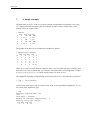
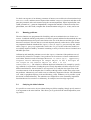
The data frame nhanes in the mice library contains example data from Schafer (1997, page
237). Suppose that the incomplete data are collected in either a matrix or data frame, where
missing values are coded as NA's.
> nhanes
age bmi hyp chl
1
1
NA NA NA
2
2 22.7
1 187
3
1
NA
1 187
4
3
NA NA NA
5
1 20.4
1 113
...
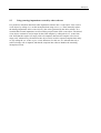
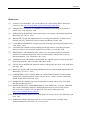
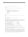
The number of the NA's can be counted and visualized as follows:
> md.pattern(nhanes)
age hyp bmi chl
13
1
1
1
1 0
1
1
1
0
1 1
3
1
1
1
0 1
1
1
0
0
1 2
7
1
0
0
0 3
0
8
9 10 27
There are 13 (out of 25) rows that are complete, there is one for which only bmi is missing, and
there are seven cases for which only age is known. The total number of missing values is equal
to (7*3)+(1*2)+(3*1)+(1*1) = 27. Most missing values (10) occur in chl.
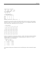
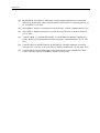
The imputation algorithm is implemented in a function called mice. The function is invoked as
> imp <- mice(nhanes)
...
which results in the object imp of a special class mids for storing multiple imputations. To see
the results of the imputation, type
> imp
Multiply imputed data set
Call:
mice(data = nhanes)
Number of multiple imputations:
Missing cells per column:
age bmi hyp chl
0
9
8 10
5
TNO report
PG/VGZ/00.038
8
Imputation methods:
age
bmi
hyp
chl
"" "pmm" "pmm" "pmm"
VisitSequence:
bmi hyp chl
2
3
4
PredictorMatrix:
age bmi hyp chl
age
0
0
0
0
bmi
1
0
1
1
hyp
1
1
0
1
chl
1
1
1
0
Random generator seed value:
0
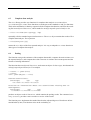
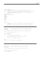
Imputations are generated according to the default method, which is predictive mean matching
(pmm) here. Entries VisitSequence and PredictorMatrix are algorithmic options that
will be discusses later. Imputations for bmi are stored in
> imp$imp$bmi
1
2
3
1 29.6 35.3 33.2
3 30.1 30.1 29.6
4 24.9 27.2 24.9
6 24.9 24.9 20.4
10 22.7 26.3 22.7
11 30.1 29.6 29.6
12 22.7 26.3 28.7
16 30.1 30.1 33.2
21 33.2 20.4 30.1
4
35.3
29.6
24.9
24.9
26.3
27.5
26.3
33.2
20.4
5
27.5
29.6
24.9
25.5
27.4
30.1
26.3
27.5
33.2
Each row corresponds to a missing entry in the bmi variable. The columns contain the different,
multiple imputations. The default number of multiple imputations is equal to five. The first
completed data set can be obtained as
> complete(imp,1)
age bmi hyp chl
1
1 29.6
1 187
2
2 22.7
1 187
3
1 30.1
1 187
4
3 24.9
1 184
5
1 20.4
1 113
...
Note that the missing entries in nhanes have now been filled by the values from the first imputation.
TNO report
PG/VGZ/00.038
9
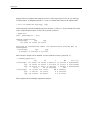
Suppose that our complete-data analysis involves a linear regression of chl on age and hyp.
For this purpose, an adapted function lm.mids is available that works on the imputed data:
> fit<-lm.mids(chl~age+hyp, imp)
which repeatedly calls the standard regression function lm. The fit object contains the results
of five complete-data analyses. These can be pooled as follows:
> pool(fit)
Call: pool(object = fit)
Pooled coefficients:
(Intercept)
age
hyp
136.2802 18.32603 20.59693
Fraction of information about the coefficients missing due to
nonresponse:
(Intercept)
age
hyp
0.2504597 0.3239345 0.4771509
More extensive output can be obtained, as usual, with the summary function, i.e.,
> summary(pool(fit))
est
se
t
(Intercept) 136.28021 28.12605 4.8453373
age 18.32603 12.45221 1.4717092
hyp 20.59693 27.84369 0.7397343
lo 95
hi 95 missing
(Intercept) 75.767847 196.79257
NA
age -9.041727 45.69378
0
hyp -44.694201 85.88807
8
This completes the full multiple imputation analysis.
df
Pr(>|t|)
13.551184 0.0002844227
11.131217 0.1687990086
7.302421 0.4825601408
fmi
0.2504597
0.3239345
0.4771509
TNO report
PG/VGZ/00.038
10
4
Specification of the imputation model
4.1
Elementary imputation methods
Data sets typically contain variables with various coding types, e.g., numerical, categorical or
binary. Some authors (Brand, 1999; Van Buuren et al, 1993, 1999; Raghunathan et al., 1998)
have proposed to specify an elementary imputation method for each variable that is to be imputed. Given the availability of these, some form of iteration can be used for obtaining imputations. Attractive aspects of this strategy are that model specification takes place on a level that is
typically well understood by the user (i.e. the individual variable), and that many methods for
creating univariate imputations are available. A disadvantage is that the properties of the combined multivariate distribution of the resulting imputations may not be known, which complicates
the assessment of convergence. See Appendix A for more details.
In mice, the user can specify an elementary imputation method for each incomplete data column. The elementary imputation method takes a set of (at that moment) complete predictors, and
returns a single imputation for each missing entry in the incomplete target column. Multiple
imputations are created by repeated calls to the function. The mice library supplies a number of
built-in elementary imputation models, which are are given in Table 4.1.
Table 4.1Built-in elementary imputation methods in mice.
Method
impute.norm
impute.pmm
impute.mean
impute.logreg
impute.logreg2
impute.polyreg
impute.lda
impute.sample
Description
Bayesian linear regression
Predictive mean matching
Unconditional mean imputation
Logistic regression
Logistic regression (direct minimization)
Polytomous logistic regression
Linear discriminant analysis
Random sample from the available observed values
Type of target
Numeric
Numeric
Numeric
2 categories
2 categories
>= 2 categories
>= 2 categories
Any
The default methods used in the mice function are impute.pmm for numeric data, impute.logreg for binary data (=factors with two categories), and impute.polyreg for
categorical variables (=factors with more than two categories). These defaults can be changed by
the defaultImputationMethod argument to the mice function. For example
> mice(nhanes, defaultImp = c("norm","logreg","polyreg"))
changes the default method for numerical data to impute.norm, while leaving the defaults for
binary and categorical data unchanged. The imputationMethod argument specifies the
imputation method per column and overides the default. This argument can be either a string or a
TNO report
PG/VGZ/00.038
11
vector of strings with length ncol(data). If imputationMethod is specified as one string,
then all visited columns will be imputed by the technique specified by this string. So
> mice(nhanes, imputationMethod = "norm")
specifies that impute.norm is to be applied on all columns. If imputationMethod is
vector of strings of length ncol(data), then each column will be imputed by the method
indicated by the position in the vector. Columns that need not be imputed have method "". For
example,
> mice(nhanes, imputationMethod = c("", "norm", "pmm", "mean"))
uses different methods for different columns. The nhanes2 data frame contains one polytomous, one binary and two numeric variables. Imputations might be created as
> imp <- mice(nhanes2, im=c("polyreg","pmm","logreg","norm"))
where polyreg is used for the first (categorical) variable, ppm for the second (numeric),
logreg for the third (binary) and norm for the fourth variable (numeric). The im parameter is a
legal S-plus abbreviation of the imputationMethod argument. Note: Running this example
produces a list of warning messages because the sample size of 25 is actually too small relative to
the number of parameters.
If the data contains factors that are used for imputing other variables, the algorithm creates
dummy variables and fills these from the corresponding factor variable. The dummy variables are
created automatically (and discarded) within the main algorithm, and are automatically imputed
where necessary.
Appendix B describes the arguments of the major functions of the mice library.
4.2
Adding your own imputation functions
It is possible to write one‘s own elementary imputation function, and call this function from
within the Gibbs sampling algorithm. The easiest way to write such a function is to copy and
modify an existing impute function, for example impute.norm. Note that this only works if
the argument list is kept intact. For more information about the proper function arguments, see
the help on impute.norm or other impute functions, e.g. by typing
> ?impute.norm
The new function can be called by the Gibbs sampler by the imputationMethod argument.
For example, calling the function impute.myfunc for each column can be done by typing
> mice(nhanes, imputationMethod="myfunc").
TNO report
PG/VGZ/00.038
12
4.3
Transformations and index variables
There is often a need for transformed, combined or recoded versions of the data. In the case of
incomplete data, one could 1) impute the original, and transform the completed original afterwards, or 2) transform the incomplete original and impute the transformed version. If, however,
both the original and the transform are needed within the imputation algorithm, neither of these
approaches work because one cannot be sure that the transformation holds between the imputed
values of the original and transformed versions.
The mice function uses a special mechanism, called 'passive imputation', to deal with such
situations. Passive imputation maintains the consistency among different transformations of the
same data. The method can be used to ensure that the transform always depends on the most
recently generated imputations in the original untransformed data. Passive imputation is invoked
by specifying a "~" as the first character of the imputation method. The entire string, including
the "~" is interpreted as the formula argument in a call to model.frame(formula,
data[!r[,j],]). This provides a simple method for specifying a large variety of dependencies among the variables, such as transformed variables, recodes, interactions, sum scores, and so
on, that may themselves be needed in other parts of the algorithm. As an example,
> imp <- mice(nhanes, imp=c("","pmm","pmm","~log(bmi)"))
replaces the missing values in the fourth column by the log of bmi, the second column. The
result is
> complete(imp)
age bmi hyp
chl
1
1 29.6
1
3.387774
2
2 22.7
1 187.000000
3
1 30.1
1 187.000000
4
3 24.9
1
3.214868
…
> complete(imp,2)
age bmi hyp
chl
1
1 29.6
1
3.387774
2
2 22.7
1 187.000000
3
1 30.1
1 187.000000
4
3 25.5
2
3.238678
Missing entries 1 and 4 in chl were replaced by the log of bmi. Note that entry 4 takes the
imputed values of bmi into account. Note also that the nonmissing values in chl are simply
copied from the data, so as a whole, the column now contains nonsensical data. One easy way to
create consistency is by coding all entries in chl as NA, but for large data sets, this can be inefficient. Another way is to apply the log transform using available cases beforehand, followed by
coding the remainder as NA.
TNO report
PG/VGZ/00.038
13
An index of more variables can be specified by means of the I() operator, e.g.
"~I(0.5*log(age)+hyp)" computes the sum of half log(age) and hypertension status:
imp <- mice(cbind(nhanes,index=NA),imp=c("","pmm","pmm","pmm",
"~I(0.5*log(age)+hyp)"))
a discretized version of the imputed variable can be obtained by
> imp_mice(cbind(nhanes,obese=NA),imp=c("","pmm","pmm","pmm",
"~cut(bmi,breaks=c(0,30,35,100))")).
and an interaction term of two variables can be created as
> imp_mice(cbind(nhanes,int=NA),imp=c("","pmm","pmm","pmm",
"~I((bmi-25)*hyp)"))
so that it is available for imputation.
There are two specific points that need attention when defining transformations through the "~"
mechanism. First, deterministic relations between columns remain synchronized if the target
variable is updated immediately after any of its predictors are imputed. So in the last example
above, column int should then be updated each time after bmi or hyp is imputed. This can be
done by changing the sequence in which the algorithm visits the columns. See section 4.4 for
more details. Second, the "~" mechanism may easily lead to linear dependencies among predictors, which produces in a fatal error if both the original and the transformed variables are simultaneously used for imputation. One can circumvent this problem by defining the set of predictors
such that original and transformed do not jointly occur. Section 4.5 described how to do this.
In S-Plus 4.5, the mice function will error if any column consists entirely of NA's. The
cbind(nhanes,index=NA) arguments creates such a data set. A workaround to the problem
is to compute the values of index for the nonmissing cases before entering the mice function.
4.4
Visiting scheme
The standard algorithm imputes each incomplete column in the data from left to right. The visitation scheme of the Gibbs sampler is essentially irrelevant as long as each column is visited often
enough, but some schemes are more efficient than others. Also, as indicated in section 4.3, the
visiting scheme plays a role in keeping relations between variables synchronised and consistent
with the current set of imputations.
It is possible to alter the default visiting scheme by the visitSequence argument of the mice
function. This is a vector of integers of arbitrary length, specifying the visiting sequence, that is,
the column order that is used to impute the data during one iteration of the algorithm. Note that a
TNO report
PG/VGZ/00.038
14
given column may be visited more than once within the same iteration. All columns with missing
data that are used as predictors should be visited, or else the function will stop with an error.
Continuing the interaction example of section 4.3, we can take care that the interaction term is
always up to date by the following command:
> imp_mice(cbind(nhanes,int=NA),imp=c("","pmm","pmm","pmm",
"~I((bmi-25)*hyp)"),visitSequence=c(2,5,3,5,4))
Using the statement, the algorithm will visits column 5 immediately after column 2 or column 3.
4.5
Choice of predictors
The argument predictorMatrix of the mice function is a square matrix of size
ncol(data) containing 0/1 data. This matrix specifying the set of predictors to be used for
each incomplete column. If diagnostics=T, then the object returned by mice contains the
predictor matrix used for imputation, e.g.
> imp$predictorMatrix
age bmi hyp chl
age
0
0
0
0
bmi
1
0
1
1
hyp
1
1
0
1
chl
1
1
1
0
Rows correspond to incomplete target variables, in the sequence as they appear in data. A value
of '1' indicates that the column variable is used as a predictor for the target (row) variable. Thus,
in the above example, age, hyp and chl are predictors for imputing bmi. The diagonal of
predictorMatrix is zero. The default setting implies that for every incomplete column all
other columns are used as predictors. However, for variables that are complete (age in the
above example) predictors are automatically removed.
The user can specify a predictorMatrix, thereby effectively limiting the number of predictors per variable. For example, suppose that bmi is not needed as a predictor. Setting all entries
in the bmi column to zero removes it from the predictor set of all other variables, e.g.
> my.predictorMatrix
age bmi hyp chl
age
0
0
0
0
bmi
1
0
1
1
hyp
1
0
0
1
chl
1
0
1
0
TNO report
PG/VGZ/00.038
15
will not use bmi as a predictor, but still impute it. The predictorMatrix argument is especially useful when dealing with data sets with a large number of variables. The next section
contains some advice regarding the selection of predictors.
4.6
General advice in choosing predictors
As a general rule, using every available bit of available information yields multiple imputations
that have minimal bias and maximal certainty. This principle implies that the number of predictors in should be chosen as large as possible. Some authors observed that including as many
predictors as possible tends to make the MAR assumption more plausible, thus reducing the need
to make special adjustments for NMAR mechanisms.
However, data sets often contain several hundreds of variables, all of which can potentially be
used to generate imputations. It is not feasible (because of multicollinearity and computational
problems) to include all these variables. It is also not necessary. In our experience, the increase in
explained variance in linear regression is typically negligible after the best, say, 15 variables have
been included. For imputation purposes, it is expedient to select a suitable subset of data that
contains no more than 15 to 25 variables. Van Buuren et al (1999) provide the following strategy
for selecting predictor variables from a large data base:
1. Include all variables that appear in the complete-data model. Failure to do so may bias the
complete-data analysis, especially if the complete-data model contains strong predictive relations. Note that this step is somewhat counter-intuitive, as it may seem that imputation would
artificially strengthen the relations of the complete-data model, which is clearly undesirable. If
done properly however, this is not the case. On the contrary, not including the complete-data
model variables will tend to bias the results towards zero.
2. In addition, include the variables that appear in the response model. Factors that are known to
have influenced the occurrence of missing data (stratification, reasons for nonresponse) are to
be included on substantive grounds. Others variables of interest are those for which the distributions differ between the response and nonresponse groups. These can be found by inspecting their correlations with the response indicator of the target variable (i.e. the variable to be
imputed). If the magnitude of this correlation exceeds a certain level, then the variable is included.
3. In addition, include variables that explain a considerable amount of variance of the target
variable. Such predictors help to reduce the uncertainty of the imputations. They are crudely
identified by their correlation with the target variable.
4. Remove from the variables selected in steps 2 and 3 those variables that have too many missing values within the subgroup of incomplete cases. A simple indicator is the percentage of
observed cases within this subgroup, the percentage of usable cases.
TNO report
16
PG/VGZ/00.038
Typically, many predictors used for imputation are incomplete themselves. In principle, one
could apply the above modelling steps for each incomplete predictor in turn, but this may lead to
a cascade of auxiliary imputation problems. In doing so, one runs the risk that every variable
needs to be included after all. In practice, there is often a small set of key variables, for which
imputations are needed, which suggests that steps 1 through 4 are to be performed for key variables only. This was the approach taken in Van Buuren, Boshuizen and Knook (1999), but it may
miss important second level predictors in the data. A safer and more efficient, though more
laborious, strategy is to perform the modeling steps for all incomplete level-1 predictors. This is
done in Oudshoorn et al. (1999). We expect that it is rarely necessary to go beyond this level.
TNO report
PG/VGZ/00.038
17
5
Running mice
5.1
Studying convergence
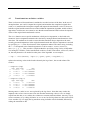
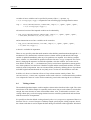
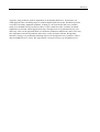
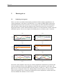
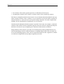
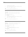
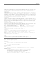
There is no clear-cut method for determining whether the Gibbs sampling algorithm has converged. Plotting the mids object (as produced by mice) yields a graphic display of the mean
and standard deviation of the imputations. On convergence, the traces should be intermingled
with each other, without showing any definite trends. Stated more precisely: convergence is
diagnosed when the variance between different sequences is no larger than the variance with each
individual sequence. Here is an example of the display that mice produces after 5 iterations:
bmi
sd
2.5
3.5
27.8
27.2
mean
4.5
28.4
bmi
2
3
4
5
1
2
3
iteration
iteration
hyp
hyp
4
5
4
5
4
5
sd
0.0
2
3
4
5
1
2
3
iteration
iteration
chl
chl
sd
180
30
200
40
220
50
1
mean
0.2
1.2
1.0
mean
0.4
1
1
2
3
iteration
4
5
1
2
3
iteration
The means (of the imputed values only) per iteration-imputation combination are plotted on the
left, the standard deviations of the imputations (within the same replication) on the right. The
plots are a bit crude because the number of missing entries is small (9, 11 and 10). It is somewhat
hard to assess convergence in this case. Plotting longer iteration sequences of more missing
entries will generally convey a better idea whether the between-imputation variability has stabilized and whether the estimates are free of trend.
TNO report
PG/VGZ/00.038
18
Note that one iteration of the algorithm involves a lot of work, e.g. for each variable and each
mutiple imputation a statistical model is fitted, imputations are drawn and data are updated. The
needed number of main iterations in mice is typically much lower than is common in modern
Markov Chain simulation techniques, that often require thousands of iterations. No iterations
need to be wasted for achieving independence in the imputations themselves, since elementary
imputation procedures create imputations that are already statistically independent for a given
value of the regression parameters. Thus, the primary function of the Gibbs sampler as implemented here, is to create independence between the posterior distributions of the regression
coefficients. The main question is whether the number of iterations is enough to stabilize the
distributions of the parameters. Brand's simulation was based on moderate amounts of missing
data and was done with just 5 iterations with satisfactory performance. (Brand, 1999). For large
amounts of missing data, convergence can be slower though. In general, we obtained good results
with as few as 5 or 10 iterations.
Note that the plot focuses on the mean and variance of the imputations. This may not correspond
to the parameter of most interest. Section 5.2 describes a more refined method for studying
convergence.
5.2
Step by step
This mice.mids function enables the user to split up the computations of the Gibbs sampler
into smaller parts by providing a stopping point after every full iteration. There are various circumstances in which this might be useful:
• Due to the way in which S-Plus handles loops, RAM memory may become easily exhausted if
the number of iterations is large. Returning to prompt/session level may alleviate these
problems;
• The user may want to compute special convergence statistics at specific points, e.g. after each
iteration, for monitoring convergence;
• For computing a 'few extra iterations'.
The imputation model itself is specified in the mice() function and cannot be changed with
mice.mids. The state of the random generator is saved with the mids-object.
As a simple example, the statements
> imp1 <- mice(nhanes,maxit=1)
> … anything you like to do here
> imp2 <- mice.mids(imp1)
yield the same result as
> imp <- mice(nhanes,maxit=2)
TNO report
PG/VGZ/00.038
19
To check convergence of an arbitrary parameter of interest, one could write a function that loops
over mice.mids, and that extracts imputed data with the complete function, and that recomputes the parameter after each iteration using the current imputations. More in particular, one
could set maxit to 1, generate imputations, compute the statistic of interest on the completed data, save the result, compute the second iteration using mice.mids, and so on.
5.3
Running problems
The mice function was programmed for flexibility, and not to minimise the use of time or resources. Combined with the greedy nature of S-Plus in general and that fact that method does not
used compiled functions, this poses some limits to the size of the data sets and the type of data
that can be analysed. The time that mice needs depends primarily on the choice of the elementary imputation methods. Methods like impute.norm or impute.pmm are fairly fast, while
others, impute.polyreg in particular, can be slow. To give an idea of the time needed, we
successfully imputed a 4000 by 20 matrix containing a variety of levels in about 15 minutes on a
400 MHz processor.
Collinearity and instability problems occur in the impute-functions if the predictors are (almost) linearly related. For example, if one predictor can be written as a linear combination of
some others, then this results in messages like Error in solve.qr(a): apparently
singular matrix and Length of longer object is not a multiple of
the length of the shorter object in: beta + rv %*%
rnorm(ncol(rv)). The solution is eliminate duplicate information, for example by specifying a reduced set of predictors. Finding the pair of nearly dependent variables can prove to be
difficult and laborious. One trick that we use in practice is to study the last eigenvector of the
covariance matrix of the incomplete data. Variables with high values on that factor often cause
the problems. Alternatively, one could revert to collinearity diagnostics like the VIF (Kleinbaum
et al, 1988) or graphical displays (Cook and Weisburg, 1999). Pedhazur (1973) provides a good
discussion on multicollinearity. The ambitious user might like to write elementary imputation
functions that are less sensitive to collinearity, for example, based on ridge regression.
5.4
Studying the initial solution
It is possible to create a mice object without doing any Gibbs sampling. Simply specify maxit=0
as an argument to the mice function. This allows you to get hold of the initial imputations (starting values).
TNO report
PG/VGZ/00.038
20
5.5
Using (starting) imputations created by other software
It is possible to transform data from other imputation software into a mids object. First create a
mids object by calling mice on the incomplete data using maxit=0. Then, manually replace
the starting imputations in the mids object by the values generated by the other software. It is
essential that external imputations are stored in the proper format of the mids object. The altered
mids object can then be used as input for the Gibbs sampler by calling the mice.mids function. Note that this requires all empty cells to be imputed, otherwise the sampler will error on
empty cells. Alternatively, the altered mids object can be used for repeated complete data analyses (by calling the lm.mids or glm.mids functions). For this use, it is allowed that only a
subset of empty cells is imputed, and that the complete data software handles the remaining
incomplete records.
TNO report
PG/VGZ/00.038
21
6
After mice
6.1
Overview
The mice library defines three data classes:
• mids: multiply imputed data set (= result of imputation)
• mira: multiply imputed repeated analyses (= results of repeated complete data analyses)
• mipo: multiple imputed pooled analysis (= result of pooling the repeated analyses)
The table below contains a short description of the key functions in the mice library.
Function
Input
Output
Description
md.pattern
data.frame
matrix
summarizes the pattern of the missing data
mice
data.frame
mids
creates a multiply imputed data set
complete
mids
data.frame converts mids into completed data
lm.mids
mids
mira
linear regression for imputed data
glm.mids
mids
mira
generalized linear model for imputed data
pool
mira
mipo
pools the repeated analyses
6.2
Extracting imputed data
The complete function extracts imputed data sets from a mids object, and returns the completed data as a data frame. For example,
> complete(imp, 3)
extracts the third complete data set from a multiply imputed data in imp. Specifying
> complete(imp, "long")
produces a long matrix where the m completed data matrices are vertically stacked and padded
with the imputation number. This form is convenient for making point estimates and for exporting multiply imputed data to other software. Other options are "broad" and "repeated",
which produce complete data in formats that are convenient for investigating between-imputation
patterns.
TNO report
PG/VGZ/00.038
22
6.3
Complete data analysis
The mice library provides two functions for complete-data analysis on a mids object:
lm.mids and glm.mids. These functions are analogues to the standard lm and glm functions.
Their main contribution is that they repeated call the complete data function, and store the resulting fits in an object of class mira, which stands for multiply imputed repeated analyses. So
> fit5<-lm.mids(chl~age+hyp, imp)
repeatedly calls the standard regression function lm. The fit5 object contains the results of five
complete-data analyses. The expression
> fit5$analyses[[1]]
returns the fit object of the first repeated analysis. It is easy to adapt the lm.mids function to
other types of complete data analysis.
6.4
Pooling
The function averages the estimates of the complete data model, computes the total variance over
the repeated analyses, and computes the relative increase in variance due to nonresponse and the
fraction of missing information.
The function takes an object of class mira, and returns an object of class mipo, which stands for
multiply imputed pooled analysis. For example,
> result <- pool(fit5)
> result
Call: pool(object = fit5)
Pooled coefficients:
(Intercept)
age
hyp
136.2802 18.32603 20.59693
Fraction of information about the coefficients missing due to
nonresponse:
(Intercept)
age
hyp
0.2504597 0.3239345 0.4771509
produces an object result of class mira, which contains the pooling results. The command summary(result)provides a more extensive overview of the results.
The function pool implements the method based on the adjusted degrees of freedom as in Barnard & Rubin (1999). The function relies on the availability of
TNO report
PG/VGZ/00.038
23
• the estimates of the model, typically present as 'coefficients' in the fit object;
• an appropriate estimate of the variance-covariance matrix of the estimates per analysis.
The latter is estimated from the fit-object by the Varcov function taken from Harrell's design
library (Alzola & Harrell, 1999). Currently, Varcov functions exists for the S-Plus standard lm
and glm function, as well as for design's specific analysis functions. For other complete data
methods, the user should define an appropriate Varcov function.
Note that not all information from the analyses is pooled. If one wants, for example, a combined
estimate of the residual variance around the regression line, this cannot be computed by the pool
function. It is however easy to adapt the pool function to other measures of interest.
Meng & Rubin (1992) describe a procedure for calculating the pooled log-likelihood ratio test
and corresponding p-value for statistical analyses on multiply imputed data. This procedure can
be used for modelling purposes in the context of generalized linear models. Appendix C contains
a worked-out example that one may adapt to apply the procedure.
TNO report
PG/VGZ/00.038
24
References
[1]
ALZOLA CF & HARRELL FE. An introduction to S-Plus and the Hmisc and Design
Libraries, 1999. http://hesweb1.med.virginia.edu/biostat/s/index.html
[2]
ARNOLD BC, CASTILLO E, SARABIA JM. Conditional specification of statistical
models. New York: Springer, 1999.
[3]
BARNARD J & RUBIN DB. Small sample degrees of freedom with multiple imputation.
Biometrika, 86, 948-955, 1999.
[4]
BRAND JPL. Design and implementation of a missing data machine. Academic thesis,
Erasmus Univerty, Rotterdam /TNO Prevention and Health, Leiden, 1999.
[5]
COOK RD & WEISBERG S. Applied regression including computing and graphics. New
York: Wiley, 1999.
[6]
GELFAND AE & SMITH AFM. Sampling-based approaches to calculating marginal
densities, Journal of the American Statistical Association, 85, 398-409, 1990.
[7]
KENNICKELL AB. Imputation of the 1989 survey of consumer finances: Stochastic
relaxation and multiple imputation, ASA 1991 Proceedings of the Section on Survey
Research Methods, 1-10. Alexandria: ASA, 1991.
[8]
KLEINBAUM DG, KUPPER LL & MULLER KE. Applied regression analysis and other
multivariate methods. 2nd Ed. Boston: PWS-Kent, 1988.
[9]
LITTLE RJA & RUBIN DB. Statistical analysis with missing data. New York: John Wiley
and Sons, 1987.
[10] MENG XL & Rubin DB. Performing likelihood ratio tests with multiple-imputed data sets.
Biometrika, 79, 103-111, 1992.
[11] OUDSHOORN CGM, VAN BUUREN S & VAN RIJCKEVORSEL. Flexible multiple
imputation by chained equations of the AVO-95 Survey. Leiden: TNO Prevention and
Health. Report PG/VGZ/99.045, 1999.
[12] PEDHAZUR EJ. Multiple regression in behavioral research. 2nd Ed. New York: Holt,
Rinehart and Winston, 1973.
[13] RAGHUNATHAN TE, SOLENBERGER PW, VAN HOEWYK J. IVEware: Imputation
and Variance Estimation Software: Installation Instructions and User Guide. Survey
Research Center, Institute of Social Research, University of Michigan, 1998.
http://www.isr.umich.edu/src/smp/ive/
[14] RUBIN DB. Multiple Imputation for Nonresponse in Surveys. New York: John Wiley and
Sons, 1987.
[15] RUBIN DB. Multiple imputation after 18+ years (with discussion), Journal of the
American Statistical Association, 91, 473-518, 1996.
TNO report
PG/VGZ/00.038
25
[16] RUBIN DB & SCHAFER JL. Efficiently creating multiple imputations for incomplete
multivariate normal data, ASA 1990 Proceedings of the Statistical Computing Section, 8388. Alexandria: ASA, 1990.
[17] SCHAFER JL. Analysis of incomplete multivariate data. London: Chapman & Hall, 1997.
[18] SCHAFER JL. Multiple imputation: A primer Statistical Methods in Medical Research,
8:3-15, 1999.
[19] VAN BUUREN S, VAN RIJCKEVORSEL JLA & RUBIN DB. Multiple imputation by
splines. Bulletin of the International Statistical Institute, Contributed Papers II, 503–504,
1993.
[20] VAN BUUREN S, BOSHUIZEN HC & KNOOK DL. Multiple imputation of missing
blood pressure covariates in survival analysis. Statistics in Medicine, 18, 681-694, 1999.
[21] VAN BUUREN S & OUDSHOORN CGM. Flexible multivariate imputation by MICE.
Leiden: TNO Preventie en Gezondheid, TNO/PG 99.054, 1999.
TNO report
PG/VGZ/00.038
26
Appendix A Imputation algorithm
Let X = (X1, X2,…, Xk) be a set of k random variables, where each variable Xj = (Xjobs, Xjmis) may
be partially observed, with j = 1,…,k. The imputation problem is to draw from P(X), the unconditional multivariate density of X. Let t denote an iteration counter. Assuming that data are missing
at random, one may repeat the following sequence of Gibbs sampler iterations:
For X1: draw imputations X1t+1 from P(X1 | X2t, X3t,…, Xkt)
For X2: draw imputations X2t+1 from P(X2 | X1t+1, X3t,…, Xkt)
:
For Xk: draw imputations Xkt+1 from P(Xk | X1t+1, X2t+1,…, Xk-1t),
i.e., condition each time on the most recently drawn values of all other variables. Properties of
this general iteration scheme have been described by Gelfand and Smith (1990). Rubin and
Schafer (1990) show that if P(X) is multivariate normal, then iterating linear regression models
like X1 = X2tβ 12 + X3tβ 13 + … + Xktβ 1k + ε1 with ε1 ~ N(0, σ12) will produce a random draw from
the desired distribution. Schafer (1997) generalizes this results to other multivariate distributions.
The implemented algorithm differs slightly from Schafer's approach in that the conditional models can be specified directly, thus without the need to choose an encompassing multivariate
model for the entire data set. It is assumed that a multivariate distribution exists, and that draws
from it can be generated by iteratively sampling from the conditional distributions. In this way,
the multivariate problem is split into a series of univariate problems. Similar ideas have been
applied by Kennickell (1991), Brand (1999), Van Buuren et al (1993, 1999) and Raghunathan et
al. (1998). Rubin coined the term ‘incompatible Gibbs’ to refer to these kinds of algorithms.
It is not always certain whether the multivariate distribution actually exists. It is possible that the
specification of two conditional distributions P(X1|X2) and P(X2|X1) are incompatible, so that no
joint distribution P(X1, X2) exists. Arnold et al. (1999) deal with this problem from a mathematical-statistical point of view. Very little is known about the properties of the Gibbs sampler under
a given incompatible specification. It could be that, since there is no distribution to converge to,
the algorithm will alternate between isolated conditional distributions. In that case, the final result
will depend on the precise stopping point, which is clearly undesirable. Things may be worse if
variables are related in a nonlinear way. Brand (1999) studied the performance of a variety of
actual algorithms based on possibly incompatible conditionals, with quite encouraging results. By
and large, the subject of incompatible Gibbs is still somewhat of an open research problem, and
more work is needed to establish its properties.
TNO report
PG/VGZ/00.038
27
Appendix B Function arguments
This appendix describes the arguments of the major functions of the mice library. For more
details on a specific function, use the standard help mechanism, e.g. by typing ?complete.
FUNCTIONS
Produces imputed flat files from multiply imputed data set (mids)
complete
DESCRIPTION:
Takes an object of type mids, fills in the missing data, and
returns the completed data in a specified format.
USAGE
data.frame <- complete(x, action=1)
REQUIRED ARGUMENTS:
x
An object of class 'mids' (created by the function mice()).
OPTIONAL ARGUMENTS:
action
If action is a scalar between 1 and x$m, the function returns the data with the action's
imputation filled in. Thus, action=1 returns the first completed data set.
The can also be one of the following strings: "long", "broad", "repeated". This
has the following meaning:
action="long" produces a long matrix with n*m rows, containing all imputed data plus two
additional variables "_ID_" (containing the row.names) and "_IMP_" (containing the imputation number).
action="broad"
produces a broad matrix with m times the number of columns in the original data. The first ncol(x$data) columns contain the first imputed data matrix. Column
names are changed to reflect the imputation number.
action="repeated" produces a broad matrix with m times ncol(x$data) columns. The first m
columns give the filled-in first variable. Column names are changed to reflect the imputation number.
VALUE:
A data frame with the imputed values filled in.
Generelized linear regression on multiply imputed data
glm.mids
DESCRIPTION:
Performs repeated glm on a multiply imputed data set
USAGE:
glm.mids(formula=formula(data), family=gaussian, data=sys.parent(), weights,
subset, na.action, start=eta, control=glm.control(...), method="glm.fit",
model=F,x=F, y=T, contrasts=NULL, ...)
TNO report
PG/VGZ/00.038
28
REQUIRED ARGUMENTS:
formula a formula expression as for other regression models, of the form
response ~ predictors. See the documentation of lm and formula for details.
data
An object of type 'mids', which stands for 'multiply imputed data set',
typically created by function mice().
OPTIONAL ARGUMENTS:
family
see glm
weights
subset
na.action
start
control
method
model
x
y
contrasts
VALUE:
An objects of class 'mira', which stands for 'multiply imputed repeated
analysis'.
This object contains m glm.objects, plus some descriptive information.
impute.lda
Elementary imputation method: Linear Discriminant Analysis
DESCRIPTION:
Imputes univariate missing data using linear discriminant analysis
USAGE:
imp <- impute.lda(y, ry, x)
REQUIRED ARGUMENTS:
y
Incomplete data vector of length n
ry
Vector of missing data pattern (F=missing, T=observed)
x
Matrix (n x p) of complete covariates.
VALUE:
imp
A vector of length nmis with imputations.
impute.logreg
Elementary imputation method: Logistic Regression
DESCRIPTION:
Imputes univariate missing data using logistic regression.
USAGE:
imp <- impute.logreg(y, ry, x)
REQUIRED ARGUMENTS:
TNO report
PG/VGZ/00.038
29
y
Incomplete data vector of length n
ry
Vector of missing data pattern of length n (F=missing, T=observed)
x
Matrix (n x p) of complete covariates.
VALUE:
imp
A vector of length nmis with imputations (0 or 1).
impute.logreg2
Elementary imputation method: Logistic Regression
DESCRIPTION:
Imputes univariate missing data using logistic regression.
USAGE:
imp <- impute.logreg2(y, ry, x)
REQUIRED ARGUMENTS:
y
Incomplete data vector of length n
ry
Vector of missing data pattern of length n (F=missing, T=observed)
x
Matrix (n x p) of complete covariates.
VALUE:
imp
A vector of length nmis with imputations (0 or 1).
impute.mean
Elementary imputation method: Simple mean imputation
DESCRIPTION:
Imputes the arithmetic mean of the observed data
USAGE:
imp <- impute.mean(y, ry, x=NULL)
REQUIRED ARGUMENTS:
y
Incomplete data vector of length n
ry
Vector of missing data pattern (F=missing, T=observed)
OPTIONAL ARGUMENTS:
x
Matrix (n x p) of complete covariates.
VALUE:
imp
A vector of length nmis with imputations.
TNO report
PG/VGZ/00.038
30
impute.norm
Elementary imputation method: Linear Regression Analysis
DESCRIPTION:
Imputes univariate missing data using linear regression analysis
USAGE:
imp <- impute.norm(y, ry, x)
REQUIRED ARGUMENTS:
y
Incomplete data vector of length n
ry
Vector of missing data pattern (F=missing, T=observed)
x
Matrix (n x p) of complete covariates.
VALUE:
imp
A vector of length nmis with imputations.
impute.pmm
Elementary imputation method: Linear Regression Analysis
DESCRIPTION:
Imputes univariate missing data using predictive mean matching
USAGE:
imp <- impute.pmm(y, ry, x)
REQUIRED ARGUMENTS:
y
Incomplete data vector of length n
ry
Vector of missing data pattern (F=missing, T=observed)
x
Matrix (n x p) of complete covariates.
VALUE:
imp
A vector of length nmis with imputations.
impute.polyreg
Elementary imputation method: Polytomous Regression
DESCRIPTION:
Imputes missing data in a categorical variable using polytomous regression
USAGE:
imp <- impute.polyreg(y, ry, x)
REQUIRED ARGUMENTS:
y
Incomplete data vector of length n
ry
Vector of missing data pattern (F=missing, T=observed)
x
Matrix (n x p) of complete covariates.
TNO report
PG/VGZ/00.038
VALUE:
imp
31
A vector of length nmis with imputations.
impute.sample
Elementary imputation method: Simple random sample
DESCRIPTION:
Imputes a random sample from the observed y data
USAGE:
imp <- impute.sample(y, ry, x=NULL)
REQUIRED ARGUMENTS:
y
Incomplete data vector of length n
ry
Vector of missing data pattern (F=missing, T=observed)
OPTIONAL ARGUMENTS:
x
Matrix (n x p) of complete covariates.
VALUE:
imp
A vector of length nmis with imputations.
lm.mids
Linear regression on multiply imputed data
DESCRIPTION:
Performs repeated linear regression on multiply imputed data set
USAGE:
fit <- lm.mids(formula, data, weights, subset, na.action, method="qr", model=F,
x=F, y=F, contrasts=NULL, ...)
REQUIRED ARGUMENTS:
formula
a formula object, with the response on the left of a ~ operator, and the
terms, separated by + operators, on the right.
data
An object of type 'mids', which stands for 'multiply imputed data set',
typically, created by function mice().
OPTIONAL ARGUMENTS:
weights
subset
na.action
method
model
x
y
contrasts
see
see
see
see
see
see
see
see
lm
lm
lm
lm
lm
lm
lm
lm
VALUE:
An objects of class 'mira', which stands for 'multiply imputed repeated
TNO report
PG/VGZ/00.038
32
analysis'.
This object contains m lm.objects, plus some descriptive information.
md.pattern
Missing data pattern
DESCRIPTION:
Computes the missing data pattern of a matrix or data.frame.
USAGE:
pat <- md.pattern(x)
REQUIRED ARGUMENTS:
x
A data frame or a matrix containing the incomplete data.
Missing values are coded as NA's.
VALUE:
A matrix with ncol(x)+1 columns, in which each row corresponds to
a missing data pattern (1=observed, 0=missing).
Rows and columns are sorted in increasing amounts of missing
information. The last column and row contain row and column counts,
respectively.
mice.mids
Multivariate Imputation by Chained Equations (iteration step)
DESCRIPTION:
Takes a "mids"-object, and produces an new object of class "mids".
USAGE:
mice.mids(obj, maxit=1, diagnostics=T, printFlag=T)
REQUIRED ARGUMENTS:
obj
An object of class "mids", typically produces by a previous call
to mice() or mice.mids()
OPTIONAL ARGUMENTS:
maxit
The number of additional Gibbs sampling iterations.
diagnostics
A Boolean flag. If TRUE, diagnostic information will be appended to
the value of the function. If FALSE, only the imputed data are saved.
The default is TRUE.
printFlag
A Boolean flag. If TRUE, diagnostic information during the Gibbs sampling
iterations will be written to the command window. The default is TRUE.
VALUE:
An object of class mids, which stands for 'multiply imputed data set'.
TNO report
PG/VGZ/00.038
mice
33
Multivariate Imputation by Chained Equations
DESCRIPTION:
Produces an object of class "mids", which stands for 'multiply imputed data set'.
USAGE:
object <- mice(data, m = 5,
imputationMethod = vector("character",length=ncol(data)),
predictorMatrix = (1 - diag(1, ncol(data))),
visitSequence = (1:ncol(data))[apply(is.na(data),2,any)],
defaultImputationMethod=c("pmm","logreg","polyreg"),
maxit = 5,
diagnostics = T,
printFlag = T,
seed = 0)
REQUIRED ARGUMENTS:
data
A data frame or a matrix containing the incomplete data. Missing values are coded as
NA's.
OPTIONAL ARGUMENTS:
m
Number of multiple imputations.
If omitted, m=5 is used.
imputationMethod
Can be either a string, or a vector of strings with length ncol(data), specifying the
elementary imputation method to be used for each column in data. If specified as a single
string, the given method will be used for all columns. The default imputation method
(when no argument is specified) depends on the measurement level of the target column and
are specified by the defaultImputationMethod argument.
Columns that need not be imputed have method "". Built-in methods are:
norm
pmm
mean
logreg
logreg2
polyreg
lda
sample
Bayesian linear regression
Predictive mean matching
Unconditional mean imputation
Logistic regression
Logistic regression (direct minimization)
Polytomous logistic regression
Linear discriminant analysis
Random sample from the observed values
Numeric
Numeric
Numeric
2 categories
2 categories
>= 2 categories
>= 2 categories
Any
For example, for the j'th column, the impute.norm function that implements the
Bayesian linear regression method can be called by specifying the string "norm"
as the j'th entry in the vector of strings.
The user can write his or her own imputation function, say impute.myfunc, and call it for
all columns by specifying imputationMethod="myfunc", or for specific columns by specifying imputationMethod=c("norm","myfunc",...).
Special method: If the first character of the elementary method is a "~", then the string
is interpreted as the formula argument in a call to model.frame(formula, data[!r[,j],]).
This provides a simple mechanism for specifying a large variety of dependencies among the
variables, for example transformed versions of imputed variables, recodes, interactions,
sum scores, and so on, that may themselves be needed in other parts of the algoritm. Note
that the "~" mechanism works only on those entries which have missing values in the
target column. The user should make sure that the combined observed and imputed parts of
the target column make sense. One easy way to create consistency is by coding all entries
in the target as NA, but for large data sets, this could be inefficient.
TNO report
PG/VGZ/00.038
34
Though not strictly needed, it is often useful to specify visitSequence such that the
column that is imputed by the "~" mechanism is visited each time after one of its predictors was visited. In that way, deterministic relation between columns will always be
synchronized.
predictorMatrix
A square matrix of size ncol(data) containing 0/1 data specifying the set of predictors
to be used for each target column. Rows correspond to target variables (i.e. variables to
be imputed), in the sequence as they appear in data. A value of '1' means that the column
variable is used as a predictor for the target variable (in the rows). The diagonal of
predictorMatrix must be zero. The default for predictorMatrix is that all other columns
are used as predictors (sometimes called massive imputation).
visitSequence
A vector of integers of arbitrary length, specifying the column indices of the visiting
sequence. The visiting sequence is the column order that is used to impute the data
during one iteration of the algorithm. A column may be visited more than once. All incomplete columns that are used as predictors should be visited, or else the function will
stop with an error. The default sequence 1:ncol(data) implies that columns are imputed
from left to right.
defaultImputationMethod=c("pmm","logreg","polyreg")
A vector of three strings containing the default imputation methods for numerical columns, factor columns with 2 levels, and factor columns with more than two levels, respectively. If nothing is specified, the following defaults will be used:
pmm
predictive mean matching
numeric data
logreg
logistic regression imputation
binary data
(factor with 2 levels)
polyreg polytomous regression imputation
categorical data (factor >= 2 levels)
maxit
A scalar giving the number of iterations. The default is 5.
diagnostics
A Boolean flag. If TRUE, diagnostic information will be appended to the value of the
function. If FALSE, only the imputed data are saved. The default is TRUE.
seed
An integer between 0 and 1000 that is used by the set.seed function for ofsetting the
random number generator. The default is 0.
VALUE:
An object of class mids, which stands for 'multiply imputed data set'. For
a description of the object, see the documentation on "mids.object".
pool
Multiple imputation pooling
DESCRIPTION:
Pools the results of m repeated complete data analysis
USAGE:
y <- pool(x, dfmethod="smallsample")
REQUIRED ARGUMENTS:
object
An object of class 'mira', produced by functions like lm.mids or glm.mids.
OPTIONAL ARGUMENTS:
dfmethod
A string describing the method to compute the degrees of freedom.
The default value is "smallsample", which specifies the is
Barnard-Rubin adjusted degrees of freedom (Barnard& Rubin, 1999)
for small samples. Specifying a different string
produces the conventional degrees of freedom as in Rubin (1987).
TNO report
PG/VGZ/00.038
35
VALUE:
An object of class 'mipo', which stands for 'multiple imputation pooled'.
DATA OBJECTS
mids
multiply imputed data set
DESCRIPTION
An object containing a multiply imputed data set
GENERATION
The "mids" object is generated by the mice and mice.mids functions.
METHODS
The "mids" class of objects has methods for the following generic functions:
print, summary, plot.
STRUCTURE
An object of class mids is a list of the following components:
call
The call that created the object.
data
A copy of the incomplete data set.
m
The number of imputations.
nmis
An array containing the number of missing observations per column.
imp
A list of nvar components with the generated multiple imputations.
Each part of the list is a nmis[j] by m matrix of imputed values for
variable j.
imputationMethod
A vector of strings of length(nvar) specifying the elementary
imputation method per column.
predictorMatrix
A square matrix of size ncol(data) containing 0/1 data specifying
the predictor set.
visitSequence
The sequence in which columns are visited.
seed
The seed value of the solution.
iteration
Last Gibbs sampling iteration number.
lastSeedValue
The most recent seed value.
chainMean
A list of m components. Each component is a length(visitSequence)
by maxit matrix containing the mean of the generated multiple
imputations. The array can be used for monitoring convergence.
Note that observed data are not present in this mean.
TNO report
PG/VGZ/00.038
36
chainCov
A list with similar structure of itermean, containing the covariances
of the imputed values.
pad
A list containing various settings of the padded imputation model,
i.e. the imputation model after creating dummy variables. Normally,
this array is only useful for error checking.
mipo
multiply imputed pooled analysis
DESCRIPTION
An object containing the m fit objects of a complete data analysis,
plus some additional information.
GENERATION
The "mipo" object is generated by the lm.mids and glm.mids functions.
METHODS
The "mipo" class of objects has methods for the following generic functions:
print, summary.
STRUCTURE
An object of class mipo is a list of the following components:
call
The call that created the mipo object.
call1
The call that created the mira object that was used in 'call'.
call2
The call that created the mids object that was used in 'call1'.
nmis
An array containing the number of missing observations per column.
m
Number of multiple imputations.
qhat
An m x npar matrix containing the complete data estimates for the
npar paremeters of the m complete data analyses.
u
An m x npar x npar array containing the variance-covariance matrices
of the m complete data analyses.
qbar
The average of complete data estimates.
ubar
The average of the variance-covariance matrix of the complete data estimes.
b
The between imputation variance-covariance matrix.
t
The total variance-covariance matrix.
r
Relative increases in variance due to missing data
df
Degrees of freedom associated with the t-statistics.
f
Fractions of missing information.
TNO report
PG/VGZ/00.038
mira
37
multiply imputed repeated analysis
DESCRIPTION
An object containing the m fit objects of a complete data analysis,
plus some additional information.
GENERATION
The "mira" object is generated by the lm.mids and glm.mids functions.
METHODS
The "mira" class of objects has methods for the following generic functions:
print, summary.
STRUCTURE
An object of class mira is a list of the following components:
call
The call that created the object.
call1
The call that created the mids object that was used in 'call'.
nmis
An array containing the number of missing observations per column.
analyses
A list of m components containing the individual fit objects
from each of the m complete data analyses.
TNO report
PG/VGZ/00.038
38
Appendix C Likelihood ratio test
##
## Reference: (1992) Meng, X., Rubin, D.B., Performing likelihood ratio tests with multiply-imputed datasets
## Biometrika, 79, pp 103-111.
imp_mice(nhanes2)
fit1_glm.mids(hyp~chl+age+bmi,data=imp)
fit0_glm.mids(hyp~age+bmi,data=imp)
formula1_hyp~chl+age+bmi
formula0_hyp~age+bmi
#### Calculate for each imputed dataset the deviance for the model
#### with and without the variable (this example: chl).
#### devM is the mean of these deviances (mean(d)'_m from the article of Meng).
deviance_0
for (i in (1:(imp$m))){
data.i_complete(imp,i)
model.0_model.matrix(formula0,data=data.i)%*%coef(fit0$analyses[[i]])
model.1_model.matrix(formula1,data=data.i)%*%coef(fit1$analyses[[i]])
deviance<-deviance+deviance.logistic(data.i$hyp,logistic(model.1))deviance.logistic(data.i$hyp,logistic(model.0))
}
devM<-deviance/imp$m
#### Calculate the pooled coefficients for the "large" and "small" model.
####
result1_pool(fit1)
result0_pool(fit0)
k<-length(result1$qbar)-length(result0$qbar)
#### Calculate now the deviance for each imputed dataset with the pooled coefficients
#### The five deviances will then be pooled: devL (mean(d)_L in the article of Meng).
deviance_0
for (i in (1:(imp$m))){
data.i_complete(imp,i)
model.0_model.matrix(formula0,data=data.i)%*%result0$qbar
model.1_model.matrix(formula1,data=data.i)%*%result1$qbar
deviance<-deviance+deviance.logistic(data.i$hyp,logistic(model.1))deviance.logistic(data.i$hyp,logistic(model.0))
}
devL<-deviance/imp$m
loglikelihoodratio(k,imp$m,devL,devM)
pooled.p.deviance(k,imp$m,devL,devM)
## The pooled loglikelihoodratio
## The pooled p-value of the loglikelihoodratio.
######################################################### functions needed
#################################
deviance.logistic<-function(yvector,fittedprobs){
yvector<-as.numeric(yvector)-1
term1_term2_rep(0,length(yvector))
term1[yvector!=0]<yvector[yvector!=0]*log(yvector[yvector!=0]/fittedprobs[yvector!=0])
term2[yvector==0]<-(1-yvector[yvector==0])*log((1-yvector[yvector==0])/(1fittedprobs[yvector==0]))
return(-(2*sum(term1+term2)))}
####
logistic<-function(mu) exp(mu)/(1+exp(mu))
####
TNO report
PG/VGZ/00.038
####
39
Calculation teststatistic D_L .
loglikelihoodratio<-function(k,nimp,devL,devM){
r.L<-((nimp+1)/(k*(nimp-1)))*(devM-devL)
return(devL/(k*(1+r.L)))}
pooled.p.deviance<-function(k,nimp,devL,devM){
r.L<-((nimp+1)/(k*(nimp-1)))*(devM-devL)
D.L<-devL/(k*(1+r.L))
nu<-k*(nimp-1)
if (nu>4) w<-4+(nu-4)*((1+(1-nu/2)*(1/r.L))^2) else w<nu*(1+1/k)*((1+1/r.L)^2)/2
return(p.value<-1-pf(D.L,k,w))}