Download User Manual

User Manual
Transcriptome Analysis
Console (TAC) Software
For Research Use Only. Not for use in diagnostic procedures.
P/N 703150 Rev. 1
Trademarks
Affymetrix®, Axiom™, Command Console®, DMET™, GeneAtlas™, GeneChip®, GeneChip-compatible™, GeneTitan®, Genotyping
Console™, NetAffx®, and Powered by Affymetrix™ are trademarks or registered trademarks of Affymetrix Inc. All other
trademarks are the property of their respective owners.
Limited License
Subject to the Affymetrix terms and conditions that govern your use of Affymetrix products, Affymetrix grants you a nonexclusive, non-transferable, non-sublicensable license to use this Affymetrix product only in accordance with the manual and
written instructions provided by Affymetrix. You understand and agree that, except as expressly set forth in the Affymetrix
terms and conditions, no right or license to any patent or other intellectual property owned or licensable by Affymetrix is
conveyed or implied by this Affymetrix product. In particular, no right or license is conveyed or implied to use this Affymetrix
product in combination with a product not provided, licensed, or specifically recommended by Affymetrix for such use.
Patents
Arrays: Products may be covered by one or more of the following patents and/or sold under license from Oxford Gene
Technology: U.S. Patent Nos. 5,445,934; 5,700,637; 5,744,305; 5,945,334; 6,054,270; 6,140,044; 6,261,776; 6,291,183; 6,346,413;
6,399,365; 6,420,169; 6,551,817; 6,610,482; 6,733,977; and EP 619 321; 373 203 and other U.S. or foreign patents.
Copyright
© 2013 Affymetrix Inc. All rights reserved.
Contents
Chapter 1
Introduction . . . . . . . . . . . . . . . . . . . . . . . . . . . . . . . . . . . . . . . . . . . . . . . . . . . 7
Transcriptome Analysis Console (TAC) . . . . . . . . . . . . . . . . . . . . . . . . . . . . . . . . . . . . . . . . . 7
Software and Hardware Requirements . . . . . . . . . . . . . . . . . . . . . . . . . . . . . . . . . . . . . . . . . 7
Installation Instructions . . . . . . . . . . . . . . . . . . . . . . . . . . . . . . . . . . . . . . . . . . . . . . . . . . . . . 7
Preferences Tab . . . . . . . . . . . . . . . . . . . . . . . . . . . . . . . . . . . . . . . . . . . . . . . . . . . . . . . . . . 8
Parts of the Preferences Window . . . . . . . . . . . . . . . . . . . . . . . . . . . . . . . . . . . . . . . . . . . . 8
Setting Up a Library Path . . . . . . . . . . . . . . . . . . . . . . . . . . . . . . . . . . . . . . . . . . . . . . . . 8
Installed Array Types . . . . . . . . . . . . . . . . . . . . . . . . . . . . . . . . . . . . . . . . . . . . . . . . . . . 9
Download Array Type Files (Internet Connection Required) . . . . . . . . . . . . . . . . . . . . . . 9
Internet Settings . . . . . . . . . . . . . . . . . . . . . . . . . . . . . . . . . . . . . . . . . . . . . . . . . . . . . 10
Algorithm Options . . . . . . . . . . . . . . . . . . . . . . . . . . . . . . . . . . . . . . . . . . . . . . . . . . . . 11
Annotation Files . . . . . . . . . . . . . . . . . . . . . . . . . . . . . . . . . . . . . . . . . . . . . . . . . . . . . 11
Alternate Splicing Analysis . . . . . . . . . . . . . . . . . . . . . . . . . . . . . . . . . . . . . . . . . . . . . . 11
Warnings . . . . . . . . . . . . . . . . . . . . . . . . . . . . . . . . . . . . . . . . . . . . . . . . . . . . . . . . . . 13
Default Button . . . . . . . . . . . . . . . . . . . . . . . . . . . . . . . . . . . . . . . . . . . . . . . . . . . . . . 13
Open Existing Result Tab . . . . . . . . . . . . . . . . . . . . . . . . . . . . . . . . . . . . . . . . . . . . . . . . . . . 13
Browsing For Existing Analysis Result . . . . . . . . . . . . . . . . . . . . . . . . . . . . . . . . . . . . . . . . 14
Chapter 2
Alternative Splicing Analysis . . . . . . . . . . . . . . . . . . . . . . . . . . . . . . . . . . . . . 16
Setting Up an Analysis Using Alt Splice CHP Files . . . . . . . . . . . . . . . . . . . . . . . . . . . . . . . . . 16
Parsing Imported Data File Names (Optional) . . . . . . . . . . . . . . . . . . . . . . . . . . . . . . . . . . 18
Importing CHP Files into Different Condition Groups . . . . . . . . . . . . . . . . . . . . . . . . . . . .20
Importing Files using Drag and Drop . . . . . . . . . . . . . . . . . . . . . . . . . . . . . . . . . . . . . . 21
Alternative Splicing Analysis Table Window (Overview) . . . . . . . . . . . . . . . . . . . . . . . . . . . . 24
Column Headers . . . . . . . . . . . . . . . . . . . . . . . . . . . . . . . . . . . . . . . . . . . . . . . . . . . . . . . 25
Showing or Hiding Table Columns . . . . . . . . . . . . . . . . . . . . . . . . . . . . . . . . . . . . . . . . 25
Sorting Columns . . . . . . . . . . . . . . . . . . . . . . . . . . . . . . . . . . . . . . . . . . . . . . . . . . . . . . . 27
Right-Click Method . . . . . . . . . . . . . . . . . . . . . . . . . . . . . . . . . . . . . . . . . . . . . . . . . . . 27
Double-Click Method . . . . . . . . . . . . . . . . . . . . . . . . . . . . . . . . . . . . . . . . . . . . . . . . . 27
Editing Filtering Properties: . . . . . . . . . . . . . . . . . . . . . . . . . . . . . . . . . . . . . . . . . . . . . 28
Clearing Filters . . . . . . . . . . . . . . . . . . . . . . . . . . . . . . . . . . . . . . . . . . . . . . . . . . . . . . . . 29
Individual Filter . . . . . . . . . . . . . . . . . . . . . . . . . . . . . . . . . . . . . . . . . . . . . . . . . . . . . . 29
All Filters . . . . . . . . . . . . . . . . . . . . . . . . . . . . . . . . . . . . . . . . . . . . . . . . . . . . . . . . . . . 29
Table Options . . . . . . . . . . . . . . . . . . . . . . . . . . . . . . . . . . . . . . . . . . . . . . . . . . . . . . . . . 29
Show Data Options . . . . . . . . . . . . . . . . . . . . . . . . . . . . . . . . . . . . . . . . . . . . . . . . . . . . . 29
Show Expressed Genes Only . . . . . . . . . . . . . . . . . . . . . . . . . . . . . . . . . . . . . . . . . . . . 29
Show Expressed PSR/JUC Only . . . . . . . . . . . . . . . . . . . . . . . . . . . . . . . . . . . . . . . . . . . 29
Have at Least One PSR . . . . . . . . . . . . . . . . . . . . . . . . . . . . . . . . . . . . . . . . . . . . . . . . .30
Showing All Data . . . . . . . . . . . . . . . . . . . . . . . . . . . . . . . . . . . . . . . . . . . . . . . . . . . . 30
Rearranging Column Orders . . . . . . . . . . . . . . . . . . . . . . . . . . . . . . . . . . . . . . . . . . . . 30
Resetting Table Defaults . . . . . . . . . . . . . . . . . . . . . . . . . . . . . . . . . . . . . . . . . . . . . . . 30
Searching Keywords . . . . . . . . . . . . . . . . . . . . . . . . . . . . . . . . . . . . . . . . . . . . . . . . . . . . 30
Exporting Options . . . . . . . . . . . . . . . . . . . . . . . . . . . . . . . . . . . . . . . . . . . . . . . . . . . . . . 31
Exporting the Current Table with 1st Gene Symbols . . . . . . . . . . . . . . . . . . . . . . . . . . 31
Contents
4
Exporting the Current Table . . . . . . . . . . . . . . . . . . . . . . . . . . . . . . . . . . . . . . . . . . . . 31
Gene Symbols to Export . . . . . . . . . . . . . . . . . . . . . . . . . . . . . . . . . . . . . . . . . . . . . . . 32
Exporting All Data . . . . . . . . . . . . . . . . . . . . . . . . . . . . . . . . . . . . . . . . . . . . . . . . . . . . 32
Saving Table Information . . . . . . . . . . . . . . . . . . . . . . . . . . . . . . . . . . . . . . . . . . . . . . . 32
Copy Selected Row(s) . . . . . . . . . . . . . . . . . . . . . . . . . . . . . . . . . . . . . . . . . . . . . . . . . 32
Copy Selected ID(s) . . . . . . . . . . . . . . . . . . . . . . . . . . . . . . . . . . . . . . . . . . . . . . . . . . . 33
Copy Selected Row(s) Gene Symbols . . . . . . . . . . . . . . . . . . . . . . . . . . . . . . . . . . . . . . 33
Copy PSR/Junction Information . . . . . . . . . . . . . . . . . . . . . . . . . . . . . . . . . . . . . . . . . . 34
Accessing External Databases (Internet Connection Required) . . . . . . . . . . . . . . . . . . . 34
Searching the Affymetrix NetAffx Website . . . . . . . . . . . . . . . . . . . . . . . . . . . . . . . . . . 35
Viewing Results in the Splicing Viewer . . . . . . . . . . . . . . . . . . . . . . . . . . . . . . . . . . . . . . . . 36
Using the Splicing Table and Splicing Viewer . . . . . . . . . . . . . . . . . . . . . . . . . . . . . . . . . . 36
Parts of the Visualization Tab . . . . . . . . . . . . . . . . . . . . . . . . . . . . . . . . . . . . . . . . . . . . . 37
Changing the Factory Set Scale Limits . . . . . . . . . . . . . . . . . . . . . . . . . . . . . . . . . . . . . 37
Setting New Scale Ranges . . . . . . . . . . . . . . . . . . . . . . . . . . . . . . . . . . . . . . . . . . . . . . 37
Changing Scale Colors . . . . . . . . . . . . . . . . . . . . . . . . . . . . . . . . . . . . . . . . . . . . . . . . 37
Find in Table . . . . . . . . . . . . . . . . . . . . . . . . . . . . . . . . . . . . . . . . . . . . . . . . . . . . . . . . 37
Parts of the Structure View . . . . . . . . . . . . . . . . . . . . . . . . . . . . . . . . . . . . . . . . . . . . . . . 38
Using the Intensity and Splicing Index Tracks with the Table . . . . . . . . . . . . . . . . . . . . 38
Using the Zoom Feature . . . . . . . . . . . . . . . . . . . . . . . . . . . . . . . . . . . . . . . . . . . . . . . 39
Using the Show Junction Option . . . . . . . . . . . . . . . . . . . . . . . . . . . . . . . . . . . . . . . . . 40
Using the Combine Neighboring Psrs Option . . . . . . . . . . . . . . . . . . . . . . . . . . . . . . . . 40
Using the Enable Tooltip Option . . . . . . . . . . . . . . . . . . . . . . . . . . . . . . . . . . . . . . . . . 40
Identifying an Alternative Splicing Event using Structure View . . . . . . . . . . . . . . . . . . . . .41
How Each Isoform Sorting Score is Calculated . . . . . . . . . . . . . . . . . . . . . . . . . . . . . . . . . 42
Parts of the Genomic View . . . . . . . . . . . . . . . . . . . . . . . . . . . . . . . . . . . . . . . . . . . . . . . 42
Using the Up and Down Regulated on Top Buttons . . . . . . . . . . . . . . . . . . . . . . . . . . . 43
Using the Show Junction Option . . . . . . . . . . . . . . . . . . . . . . . . . . . . . . . . . . . . . . . . . 43
Using the Truncate Intronic Region Option . . . . . . . . . . . . . . . . . . . . . . . . . . . . . . . . . 44
Using the Enable Tooltip Option . . . . . . . . . . . . . . . . . . . . . . . . . . . . . . . . . . . . . . . . . 44
Using the Zoom Feature . . . . . . . . . . . . . . . . . . . . . . . . . . . . . . . . . . . . . . . . . . . . . . . 44
Selecting Different Transcript Isoforms IDs (Internet Connection Required) . . . . . . . . . . 44
Linking Isoforms to an External Source (Internet Access Required) . . . . . . . . . . . . . . . . 44
How Transcript Isoforms are Sorted . . . . . . . . . . . . . . . . . . . . . . . . . . . . . . . . . . . . . . . 45
Linking Out to the UCSC Genome Browser (Internet Access Required) . . . . . . . . . . . . . 45
Using the Get Score Button . . . . . . . . . . . . . . . . . . . . . . . . . . . . . . . . . . . . . . . . . . . . . 46
Chapter 3
Gene Level Differential Expression Analysis . . . . . . . . . . . . . . . . . . . . . . . . 47
Setting Up an Analysis Using Gene CHP Files . . . . . . . . . . . . . . . . . . . . . . . . . . . . . . . . . . . 47
Parsing Imported Data File Names (Optional) . . . . . . . . . . . . . . . . . . . . . . . . . . . . . . . . . . 49
Importing CHP Files into Different Condition Groups . . . . . . . . . . . . . . . . . . . . . . . . . . . .50
Importing Files using Drag and Drop . . . . . . . . . . . . . . . . . . . . . . . . . . . . . . . . . . . . . . 51
Column Headers . . . . . . . . . . . . . . . . . . . . . . . . . . . . . . . . . . . . . . . . . . . . . . . . . . . . . . . 56
Showing or Hiding Table Columns . . . . . . . . . . . . . . . . . . . . . . . . . . . . . . . . . . . . . . . . 56
Right-Click Method . . . . . . . . . . . . . . . . . . . . . . . . . . . . . . . . . . . . . . . . . . . . . . . . . . . 57
Double-Click Method . . . . . . . . . . . . . . . . . . . . . . . . . . . . . . . . . . . . . . . . . . . . . . . . . 57
Filtering Column Data . . . . . . . . . . . . . . . . . . . . . . . . . . . . . . . . . . . . . . . . . . . . . . . . . . . 57
Editing Filtering Properties: . . . . . . . . . . . . . . . . . . . . . . . . . . . . . . . . . . . . . . . . . . . . . 58
Clearing Filters . . . . . . . . . . . . . . . . . . . . . . . . . . . . . . . . . . . . . . . . . . . . . . . . . . . . . . . . 58
Individual Filter . . . . . . . . . . . . . . . . . . . . . . . . . . . . . . . . . . . . . . . . . . . . . . . . . . . . . . 58
All Filters . . . . . . . . . . . . . . . . . . . . . . . . . . . . . . . . . . . . . . . . . . . . . . . . . . . . . . . . . . . 59
Contents
5
Table Options . . . . . . . . . . . . . . . . . . . . . . . . . . . . . . . . . . . . . . . . . . . . . . . . . . . . . . . . . 59
Rearranging Factory Set Columns . . . . . . . . . . . . . . . . . . . . . . . . . . . . . . . . . . . . . . . . . . 59
Reset to Default . . . . . . . . . . . . . . . . . . . . . . . . . . . . . . . . . . . . . . . . . . . . . . . . . . . . . . .59
Searching Keywords . . . . . . . . . . . . . . . . . . . . . . . . . . . . . . . . . . . . . . . . . . . . . . . . . . . . 59
Exporting Options . . . . . . . . . . . . . . . . . . . . . . . . . . . . . . . . . . . . . . . . . . . . . . . . . . . . . . 60
Exporting the Current Table with 1st Gene Symbols . . . . . . . . . . . . . . . . . . . . . . . . . . 60
Gene Symbols to Export . . . . . . . . . . . . . . . . . . . . . . . . . . . . . . . . . . . . . . . . . . . . . . . 61
Exporting All Data . . . . . . . . . . . . . . . . . . . . . . . . . . . . . . . . . . . . . . . . . . . . . . . . . . . . 61
Saving Table Information . . . . . . . . . . . . . . . . . . . . . . . . . . . . . . . . . . . . . . . . . . . . . . . 61
Copy Selected ID(s) . . . . . . . . . . . . . . . . . . . . . . . . . . . . . . . . . . . . . . . . . . . . . . . . . . . 62
Copy Selected Row(s) Gene Symbols . . . . . . . . . . . . . . . . . . . . . . . . . . . . . . . . . . . . . . 62
Accessing External Databases (Internet Connection Required) . . . . . . . . . . . . . . . . . . . 63
Searching the Affymetrix NetAffx Website . . . . . . . . . . . . . . . . . . . . . . . . . . . . . . . . . . 63
Gene Level Differential Expression Analysis Graphs . . . . . . . . . . . . . . . . . . . . . . . . . . . . . . . 64
Scatter Plot Graph (Overview) . . . . . . . . . . . . . . . . . . . . . . . . . . . . . . . . . . . . . . . . . . . . . 64
Using the Table to Investigate Lassoed Selections . . . . . . . . . . . . . . . . . . . . . . . . . . . . . 65
Clearing Lassoed Selections . . . . . . . . . . . . . . . . . . . . . . . . . . . . . . . . . . . . . . . . . . . . . 66
Changing Graph Colors . . . . . . . . . . . . . . . . . . . . . . . . . . . . . . . . . . . . . . . . . . . . . . . . 66
Volcano Plot Graph (Overview) . . . . . . . . . . . . . . . . . . . . . . . . . . . . . . . . . . . . . . . . . . . . 67
Lassoing Genes of Interest . . . . . . . . . . . . . . . . . . . . . . . . . . . . . . . . . . . . . . . . . . . . . . 68
Using the Table to Investigate Lassoed Selections . . . . . . . . . . . . . . . . . . . . . . . . . . . . . 69
Copying Lassoed Selections . . . . . . . . . . . . . . . . . . . . . . . . . . . . . . . . . . . . . . . . . . . . . 69
Clearing Lassoed Selections . . . . . . . . . . . . . . . . . . . . . . . . . . . . . . . . . . . . . . . . . . . . . 70
Changing Graph Colors . . . . . . . . . . . . . . . . . . . . . . . . . . . . . . . . . . . . . . . . . . . . . . . . 70
Chromosome Summary Graph (Overview) . . . . . . . . . . . . . . . . . . . . . . . . . . . . . . . . . . . . 71
Using the Table to Investigate Pre-Lassoed Selections . . . . . . . . . . . . . . . . . . . . . . . . . . 73
Copying Lassoed Selections . . . . . . . . . . . . . . . . . . . . . . . . . . . . . . . . . . . . . . . . . . . . . 73
Clearing Lassoed Selections . . . . . . . . . . . . . . . . . . . . . . . . . . . . . . . . . . . . . . . . . . . . . 74
Changing Graph Colors . . . . . . . . . . . . . . . . . . . . . . . . . . . . . . . . . . . . . . . . . . . . . . . . 74
Hierarchical Clustering Graph . . . . . . . . . . . . . . . . . . . . . . . . . . . . . . . . . . . . . . . . . . . . . 75
Selecting Interesting Probe Sets . . . . . . . . . . . . . . . . . . . . . . . . . . . . . . . . . . . . . . . . . .76
Exporting Probe Sets of Interest . . . . . . . . . . . . . . . . . . . . . . . . . . . . . . . . . . . . . . . . . .78
Changing Graph Colors . . . . . . . . . . . . . . . . . . . . . . . . . . . . . . . . . . . . . . . . . . . . . . . . 78
Obtaining Information Related to Individual Probe Sets . . . . . . . . . . . . . . . . . . . . . . . . 79
Conditions . . . . . . . . . . . . . . . . . . . . . . . . . . . . . . . . . . . . . . . . . . . . . . . . . . . . . . . . . 79
Signal Intensity Scale . . . . . . . . . . . . . . . . . . . . . . . . . . . . . . . . . . . . . . . . . . . . . . . . . . 80
Saving a Hierarchical Cluster . . . . . . . . . . . . . . . . . . . . . . . . . . . . . . . . . . . . . . . . . . . . 80
Printing Option . . . . . . . . . . . . . . . . . . . . . . . . . . . . . . . . . . . . . . . . . . . . . . . . . . . . . . 80
Chapter 4
Exon Level Differential Expression Analysis . . . . . . . . . . . . . . . . . . . . . . . . . 81
Setting Up an Analysis Using Exon CHP Files . . . . . . . . . . . . . . . . . . . . . . . . . . . . . . . . . . . . 81
Parsing Imported Data File Names (Optional) . . . . . . . . . . . . . . . . . . . . . . . . . . . . . . . . . . 83
Importing CHP Files into Different Condition Groups . . . . . . . . . . . . . . . . . . . . . . . . . . . .83
Importing Files using Drag and Drop . . . . . . . . . . . . . . . . . . . . . . . . . . . . . . . . . . . . . . 84
Exon Level Differential Expression Analysis Summary Window (Overview) . . . . . . . . . . . . . . 85
Exon Level Differential Expression Analysis Table Window (Overview) . . . . . . . . . . . . . . . . . 87
Column Headers . . . . . . . . . . . . . . . . . . . . . . . . . . . . . . . . . . . . . . . . . . . . . . . . . . . . . . . 88
Sorting Columns . . . . . . . . . . . . . . . . . . . . . . . . . . . . . . . . . . . . . . . . . . . . . . . . . . . . . . . 89
Right-Click Method . . . . . . . . . . . . . . . . . . . . . . . . . . . . . . . . . . . . . . . . . . . . . . . . . . . 90
Double-Click Method . . . . . . . . . . . . . . . . . . . . . . . . . . . . . . . . . . . . . . . . . . . . . . . . . 90
Contents
6
Filtering Column Data . . . . . . . . . . . . . . . . . . . . . . . . . . . . . . . . . . . . . . . . . . . . . . . . . . . 90
Editing Filtering Properties: . . . . . . . . . . . . . . . . . . . . . . . . . . . . . . . . . . . . . . . . . . . . . 91
Clearing Filters . . . . . . . . . . . . . . . . . . . . . . . . . . . . . . . . . . . . . . . . . . . . . . . . . . . . . . . . 91
Individual Filter . . . . . . . . . . . . . . . . . . . . . . . . . . . . . . . . . . . . . . . . . . . . . . . . . . . . . . 91
All Filters . . . . . . . . . . . . . . . . . . . . . . . . . . . . . . . . . . . . . . . . . . . . . . . . . . . . . . . . . . . 92
Table Options . . . . . . . . . . . . . . . . . . . . . . . . . . . . . . . . . . . . . . . . . . . . . . . . . . . . . . . . . 92
Rearranging Column Orders . . . . . . . . . . . . . . . . . . . . . . . . . . . . . . . . . . . . . . . . . . . . 92
Resetting Table Defaults . . . . . . . . . . . . . . . . . . . . . . . . . . . . . . . . . . . . . . . . . . . . . . . 92
Searching Keywords . . . . . . . . . . . . . . . . . . . . . . . . . . . . . . . . . . . . . . . . . . . . . . . . . . . . 92
Changing Condition vs. Condition Pairings . . . . . . . . . . . . . . . . . . . . . . . . . . . . . . . . . . . 92
Exporting Options . . . . . . . . . . . . . . . . . . . . . . . . . . . . . . . . . . . . . . . . . . . . . . . . . . . . . . 93
Exporting the Current Table with 1st Gene Symbols . . . . . . . . . . . . . . . . . . . . . . . . . . 93
Exporting the Current Table . . . . . . . . . . . . . . . . . . . . . . . . . . . . . . . . . . . . . . . . . . . . 93
Exporting All Data . . . . . . . . . . . . . . . . . . . . . . . . . . . . . . . . . . . . . . . . . . . . . . . . . . . . 94
Saving Table Information . . . . . . . . . . . . . . . . . . . . . . . . . . . . . . . . . . . . . . . . . . . . . . . 94
Copy Selected Row(s) . . . . . . . . . . . . . . . . . . . . . . . . . . . . . . . . . . . . . . . . . . . . . . . . . 94
Copy Selected ID(s) . . . . . . . . . . . . . . . . . . . . . . . . . . . . . . . . . . . . . . . . . . . . . . . . . . . 94
Copy Selected Row(s) Gene Symbols . . . . . . . . . . . . . . . . . . . . . . . . . . . . . . . . . . . . . . 95
Copy Exon Information . . . . . . . . . . . . . . . . . . . . . . . . . . . . . . . . . . . . . . . . . . . . . . . . 95
The selected exons are now copied to the Windows Clipboard for pasting. . . . . . . . . . 96
Accessing External Databases (Internet Connection Required) . . . . . . . . . . . . . . . . . . . 96
Searching the Affymetrix NetAffx Website . . . . . . . . . . . . . . . . . . . . . . . . . . . . . . . . . . 96
Appendix A
Algorithms . . . . . . . . . . . . . . . . . . . . . . . . . . . . . . . . . . . . . . . . . . . . . . . . . . . 97
1) Tukey's Bi-weight Average Algorithm . . . . . . . . . . . . . . . . . . . . . . . . . . . . . . . . . . . . . 97
2) ANOVA and Standard Deviation are Calculated using NMATH Package . . . . . . . . . . . . 97
3) Chromosome Naming Scheme . . . . . . . . . . . . . . . . . . . . . . . . . . . . . . . . . . . . . . . . . . 97
4) Splicing Index (SI) Algorithm . . . . . . . . . . . . . . . . . . . . . . . . . . . . . . . . . . . . . . . . . . . . 98
Performing an Alternate Splicing Analysis . . . . . . . . . . . . . . . . . . . . . . . . . . . . . . . . . . 98
5) Benjamini-Hochberg Step-Up FDR-controlling Procedure . . . . . . . . . . . . . . . . . . . . . . . 99
6) Fold Change . . . . . . . . . . . . . . . . . . . . . . . . . . . . . . . . . . . . . . . . . . . . . . . . . . . . . . .100
7) Hierarchical Clustering . . . . . . . . . . . . . . . . . . . . . . . . . . . . . . . . . . . . . . . . . . . . . . .100
1
Introduction
Transcriptome Analysis Console (TAC)
TAC performs statistical analysis to obtain a list of differentially expressed genes and alternative splicing
events. IT also provides the visualization of genes, exons, junctions and transcript isoforms. TAC runs
analysis based on Expression Console (EC) generated CHP files.
NOTE: Affymetrix recommends that if you are using GCOS CEL files, you should use the Data
Transfer Tool (DTT) provided by Affymetrix to move the CEL files out of the GCOS directory.
Software and Hardware Requirements
The table below shows the operating systems the recommended minimum requirements. (Table 1.1)
IMPORTANT: Larger data file sizes associated with Whole Transcriptome arrays should be
taken into account when calculating the necessary available disk space requirement.
Larger data file sizes associated with Whole Transcriptome arrays should be taken into account when
calculating the necessary available disk space requirement.
Table 1.1 System Requirements
64-bit Operating System
Speed
Memory
(RAM)
Available Disk
Space*
Web Browser
Microsoft Windows® 7 professional
8 GHz Intel Pentium
operating system with Service Pack 1 Quad Core Processor
16 GB RAM
150 GB HD +
data storage
IE 7.0 and above
Microsoft Windows® XP operating
system with Service Pack 2.0
8 GB RAM
150 GB HD +
data storage
IE 7.0 and above
4 GHz Intel Pentium
Quad Core Processor
Recommended: 16 GB of RAM.
Installation Instructions
To install the Transcriptome Analysis Console software:
1. Go to www.affymetrix.com and navigate to the following location:
Home > Products > Microarray Solutions > Instruments and Software > Software >
2. Locate and download the zipped TAC software package.
3. Unzip the file, then double-click TAC64.exe to install it.
4. Follow the directions provided by the installer.
The setup process includes and installs the required Microsoft component,.NET Framework 4 Client
Profile.
Chapter 1 | Introduction
8
Preferences Tab
Use the Preferences tab to setup or change a library path, download library and annotation files, and
modify algorithm options. (Figure 1.1)
Figure 1.1 Main Preferences window
Parts of the Preferences Window
Setting Up a Library Path
IMPORTANT: The first time you install TAC, you must assign a path to your library folder. The
library folder contains the library and annotation files required to run the TAC software.
Figure 1.2 Library Path
Do the following to create a new Library Path:(Figure 1.2)
1. Click
(right side of library path) to create a new library folder path.
Chapter 1 | Introduction
9
The following Browse For Folder window appears. (Figure 1.3)
Figure 1.3 Browse For Folder
2. Click New Folder to choose a new Library folder. Name the new folder, then click OK.
Installed Array Types
Displays the currently installed array types inside your library folder. (Figure 1.4)
Figure 1.4 Installed Array Types
Download Array Type Files (Internet Connection Required)
1. Click Download Array Type Files to download library and annotation files from Affymetrix.com.
The NetAffx Account Information dialog window appears.
2. Enter your Netaffx account email and password, then click OK or click the Register Now link to
obtain a new account.
Do the following to download library and/or annotation files:
1. Click
.
The NetAffx Account Login window appears. (Figure 1.5)
Figure 1.5 NetAffx Account Login
2. Enter your NetAffx email and password, then click OK.
Chapter 1 | Introduction
10
The following window appears; (Figure 1.6)
Figure 1.6 NetAffx Library Files
3. Click the checkbox next to the library file(s) you want to download, then click Download.
A progress bar appears, then the downloaded library and annotation file(s) appear in the Installed Array
Types panel.
Internet Settings

To enable the Internet Settings option, click on the down-arrow button. (Figure 1.7)
Figure 1.7 Internet Settings

If you are using a Proxy Server, click its checkbox, then complete the required fields. (Figure 1.8)
Figure 1.8 Internet Settings - Proxy Server Information
Chapter 1 | Introduction
11
Algorithm Options

To customize Algorithm Options, click on the down-arrow button. (Figure 1.9)
Figure 1.9 Algorithm Options Drop-down
If you have more than one array type installed and you want to change algorithm options for another
array, use the drop-down menu to select a different array. (Figure 1.10)
Figure 1.10 Algorithm Options
Annotation Files
Use the drop-down menus to select different versions of annotation files for various types of analysis.
(Figure 1.11)
Figure 1.11 Annotation Files
Alternate Splicing Analysis
Here you can customize algorithm parameters by typing values in the text boxes (Figure 1.12).
NOTE: Alternate Splicing Analysis is only available for certain arrays. Please contact
Affymetrix support regarding which array is supported.
Figure 1.12 Configurable Parameters 1-5
1
2
3
4
5
Chapter 1 | Introduction
12
The Splicing Index algorithm compares normalized signal estimates from one condition to another. See
the equation below: (Figure 1.13)
Figure 1.13 Splicing Index Algorithm
In order for Transcriptome Analysis Console to perform a Splicing Index, two key criteria must be met.
They are as follows:
1. Criteria 1: A Transcript Cluster gene must be expressed in both conditions. Therefore, for each



condition, you need to determine whether a gene is expressed or not.
Configurable Parameter 3: A gene can be considered expressed in a condition (if it meets the criteria
specified in parameter 3. As an example, if at least 50% of the samples are expressed, then this gene is
expressed in this condition).
Configurable Parameter 2: You must determine whether a gene is expressed by looking at the DABG
p-values for all the eligible exons (PSRs). As an example, at least 50% of eligible PSRs must be
expressed (DABG p < 0.05) for the gene to be considered expressed.
Configurable Parameter 1: The way to decide whether a PSR is eligible, is to see if it presents at least
50% of all the transcript isoforms for that gene. Only PSRs 1, 2, 3, 4, 8 are considered as eligible PSRs
in this gene, as shown in the example below. (Figure 1.14)
Figure 1.14 Configurable Parameters
2. Criteria 2: A PSR or Junction can only be analyzed by Splicing Index if it expresses in at least one





condition
Configurable Parameter 4: To decide whether a PSR or junction is expressed in a condition, you need
(as an example) to check the DABG p-values (from all samples in that condition) to see whether>=50%
of samples have DABG p < 0.05.
After a gene and PSRs/junctions meet the criteria above - normalization and comparison can begin.
In order to perform normalization, gene intensity needs to be calculated. For a particular gene, the gene
intensity for each sample is calculated using the Tukey's Biweight average for all the eligible exons
(PSRs) intensities in that gene.
Next, normalize each PSR or junction intensity using the gene intensity of that sample. (Figure 1.13)
Normalized intensities from Condition1 is compared to normalized intensities from condition 2 using
One-way Between-Subject ANOVA for the PSRs and junctions within a gene.
Chapter 1 | Introduction
13
Configurable Parameter 5:After running ANOVA, multi-testing correction is performed using
Benjamini-Hochberg Step-Up FDR-controlling procedure for all the expressed genes and expressed
PSRs/Junctions (expressed in at least one condition).

NOTE: By default, the Alpha level is set as 0.05 in Parameter 5 (False Discovery Rate field).
Warnings
If algorithm parameters have been changed to other values than default, red warning text appears at the
bottom of the Preferences window. Below are two warning examples: (Figure 1.15)
Figure 1.15 Warnings
2
1
1. A blank/non-number entry generates a is not a number! warning.
2. Parameter(s) entered, that are different from the default generate a Parameter(s) are different than
the defaults! warning.
NOTE: Warnings are not analysis specific. Example: If you change parameters for a splicing
index, then run a gene level analysis, any change warnings remain on screen (regardless if
your parameter setting applies to your analysis or not).
Default Button
Click Default (bottom right) to RESET Algorithm parameters to their factory settings.
Open Existing Result Tab
TAC always auto-saves your studies. At any time, you can view recent analysis results.
1. Click on the Open Existing Result tab.
TIP: Click any of the window’s header columns to sort your recent studies by Ascending
(A-Z) or Sort By Descending (Z-A).
Chapter 1 | Introduction
14
The Open Existing Result window appears. (Figure 1.16)
Figure 1.16 Open Existing Result window
2. Double-click on a recent study or single-click on it, then click
.
After a few moments, your recent study opens (in the same state - you last left it).
Browsing For Existing Analysis Result
Do the following if you cannot locate a study:
1. TAC stores twenty recent results in the Open Existing Result window. If you still cannot locate your
study, click
.
Chapter 1 | Introduction
15
The following window appears: (Figure 1.17)
Figure 1.17 TAC Analysis Results window
2. Click on a recent study from the TAC Analysis Results window, then click Open.
After a few moments, your recent study opens (in the same state - you last left it).
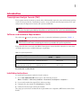
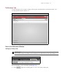
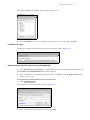
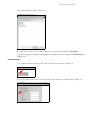
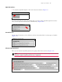
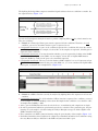
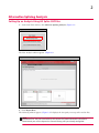
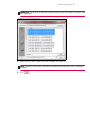
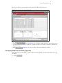
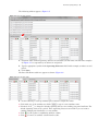
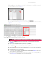
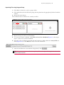
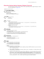
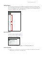
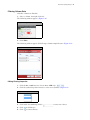
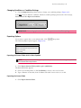
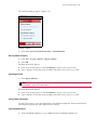
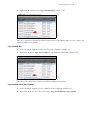
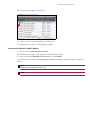
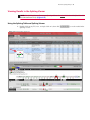
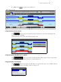
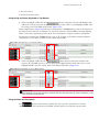
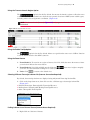
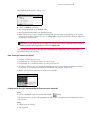
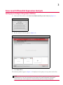
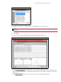
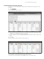
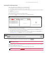
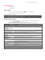
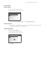
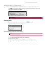
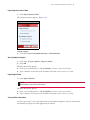
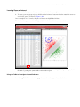
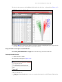
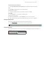
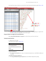
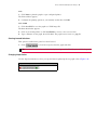
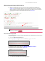
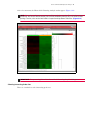
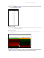
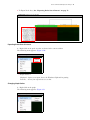
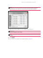
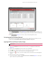
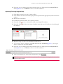
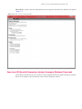
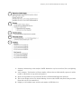
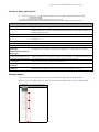
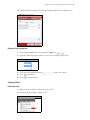
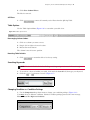
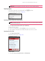
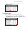
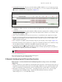
2
Alternative Splicing Analysis
Setting Up an Analysis Using Alt Splice CHP Files
1. At the main TAC window, click Alternate Splicing Analysis. (Figure 2.1)
Figure 2.1 Main TAC window
The New Analysis window appears. (Figure 2.2)
Figure 2.2 New Analysis window
2. Click Import Data.
The following window appears. (Figure 2.3) It displays the data path you set up earlier and its files.
NOTE: The first time you launch TAC, it asks you to define a path to store your library and
annotation files. For your convenience, TAC retains this path information. Affymetrix
recommends you use the Expression Console library path you already configured.
Alternative Splicing Analysis
17
IMPORTANT: To perform an alternative splicing analysis, you must import “alt-splice” .chp
files. (Figure 2.3)
Figure 2.3 Import Data Dialog window
3. Single click, Ctrl click, or Shift click to select multiple files (Figure 2.3).
NOTE: To optimize the analysis, Affymetrix recommends importing more than 1 sample per
condition.
4. Click
.
Alternative Splicing Analysis
18
The selected files are now populated in the Sample File Window. (Figure 2.4)
Figure 2.4 Import Data into Sample File Window


Click
checkbox (Figure 2.4) to display sample file names and attributes (even
after they have been added to conditions). Samples that have been added to different conditions are
displayed in gray.
Click
(Figure 2.4) to remove a file(s) from the Sample File window.
Parsing Imported Data File Names (Optional)
This option gives you the ability to parse attributes from the sample file names and helps you set up
conditions.
1. Click
.
Alternative Splicing Analysis
19
The following window appears: (Figure 2.5)
Figure 2.5 Parse File Name window
2. Determine what common separating characters reside within your file names. The file name examples
(in Figure 2.5) are separated by an underscore and period.
3. Type the appropriate symbols in the Separating Characters field. In this example, an underscore and
period.
4. Click Parse.
The Parse File Names table now appears as shown. (Figure 2.6)
Figure 2.6 Parse File Name table
5. Do the following to clean up attributes parsed from the sample file names:




Click inside any of the Attribute text fields
to type in a new Attribute name.
If desired, click
to change the default separating character for combing your parsed attributes. The
default separating character is a period. These separating characters are useful if you ever want to
combine multiple parsed attributes to a new attribute.
Click
to join together a neighboring attribute column.
Click
to remove an attribute column from the table.
Alternative Splicing Analysis
20
In the example above, since Attribute 1, 3, 4, 5, and 7 are redundant and not useful, they are removed.
The table now appears as shown. (Figure 2.7)
Figure 2.7 Parse File Name table with 2 attributes
6. To save your parsed attributes to the Same File window, click
.
The parsed file name attributes (Figure 2.7) are added to the Sample File window as additional attributes.
(Figure 2.8)
Figure 2.8 Parsed results reflected in the Sample File window
Importing CHP Files into Different Condition Groups
IMPORTANT: Customize your condition names first, then add the CHP files into each condition.
1. Click on the Condition1 window header field to rename it to an appropriate Condition name.
(Figure 2.9)
2. Click to select and highlight the data you want to use for Condition1.
3. Click
in the Condition1 window to add your selected files to the Condition1 window.
4. If needed, click
5. If needed, click
to move selected files back to the Sample File window.
to delete your current Condition and move all its files back to the Sample File
window.
6. Repeat the steps 1-3 (above) for Condition2.
7. To create more than 2 conditions, click Click to Create New Condition (Figure 2.9), then repeat
steps 1-3 (above) for your 3rd Condition.
8. If needed, edit your Analysis result file path and/or name by clicking inside the Analysis File text
field (Figure 2.10), or click Browse to select a new file destination.
Alternative Splicing Analysis
21
Importing Files using Drag and Drop
1. Click Shift or click Ctrl, to select a group of files.
2. Click and hold onto the last file in the group, then drag them into the appropriately labeled Condition
window.
3. Release the mouse button.
The Condition1 (Liver) window now contains your files.
Figure 2.9 Edited Condition1 name with samples
4. Repeat the steps 1-3 (above) for Condition2.
5. To create more than 2 conditions, click Click to Create New Condition (Figure 2.9), then repeat
steps 1-3 (above) for your 3rd Condition.
6. If needed, edit your Analysis result file path and/or name by clicking inside the Analysis File text
field (Figure 2.10), or click Browse to select a new file destination.
Figure 2.10 Editable Analysis Result File Paths
7. After the Conditions have been labeled and populated, click
.
TIP: TAC auto-saves your studies. At any time, click on the Open Existing Result tab to view
recent analysis results.
Alternative Splicing Analysis
22
Please Wait... appears. then (by default), the Summary and the Splicing Viewer appear together using a
split window view. (Figure 2.11)
Figure 2.11 Summary and Splicing Viewer
Alternative Splicing Analysis
23
Alternative Splicing Analysis Summary Window (Overview)
The information shown in the summary is based on the algorithm parameters applied during the analysis.
See the example below: (Figure 2.12)
Figure 2.12 Summary Window
1
2
3
4
5
6
1. Summary information per this Alternative Splicing Analysis. NOTE: Summaries vary between Gene,
Exon, and Splicing analysis.
2. Array summary. Total number of transcript clusters (genes), and numbers of coding and noncoding
transcript clusters on this array.
3. Summary of the Coding transcript clusters. In the example above, 33723 transcript clusters passed the
Splicing Index criteria of Genes need to be expressed in both conditions. 8270 transcript clusters
have at least one Probe Selection Region (PSR) with Splicing Index (linear) < -2 or Splicing Index
(linear) > 2. The group of genes listed below (2059, 2565, and 6360) represent the genes that do not
meet the Splicing Index criteria of Genes need to be expressed in both conditions.
Alternative Splicing Analysis
24
4. Displays the algorithm parameters used to perform the splicing analysis.
5. This section displays the factory default filtering criteria results. NOTE: Only transcript clusters that
pass in the Splicing table criteria are summarized.
6. Displays each Condition name and the total number of CHP files in it. Scroll down to reveal the other
Conditions in your analysis.
Alternative Splicing Analysis Table Window (Overview)
The table results are based on the algorithm parameters applied during the analysis. The information
shown is divided into 2 parts. (Figure 2.13)


The left side of the table provides gene level information.
The right side of the table provides PSR/Junction information and is organized by each transcript
cluster.
Figure 2.13 Table window
Alternative Splicing Analysis
25
Parts of the Table


Column Headers
Table Options
Column Headers
The factory default columns and 2 preset filters
are as shown. (Figure 2.14)
See Table 2.1 for definitions of these columns.
Figure 2.14 Default Table Column Headers
Showing or Hiding Table Columns
1. Click the
drop-down menu to show or hide columns in the splicing table.
2. Click outside the Show/Hide Drop-down menu to close it.
Table 2.1 Available Splicing Table Columns (BOLD columns represents columns that TAC displays by default)
Available Columns
Description
Transcript Cluster ID
ID of Transcript Cluster (TC)
(Condition1) Expressed
(Condition2) Expressed
True or False statement regarding whether this TC is expressed in a condition based on criteria
specified in the Algorithm Options.
As an example, True means >= 50% samples are expressed in this condition
False means < 50% samples are expressed in this condition
(Condition1) Expressed (Detail)
(Condition2) Expressed (Detail)
Number of expressed samples/total samples in a condition.
As an example, 4/4 means 4 out of 4 samples met this criteria: >=50% eligible PSRs have DABG
< 0.05
1/4 means only 1 out of 4 samples met this criteria: >=50% eligible PSRs have DABG < 0.05
(Condition1) Gene Avg Signal
(log2)
(Condition2) Gene Avg Signal
(log2)
Tukey's Bi-weight1 average of gene level intensity of all the samples in a condition:
Bi-weight average of (sample 1 gene1 intensity + sample 2 gene1 intensity +…+ sample N gene1
intensity)
(Condition1) Standard Deviation
(Condition2) Standard Deviation
Standard Deviation2 of gene intensities from all samples in a condition:
STDEV of (sample 1 gene1 intensity + sample 2 gene1 intensity +…+ sample N gene1 intensity)
Gene Fold Change (linear)
(Condition1 vs. Condition2)
This shows the fold change (in linear space) of Condition1 vs. Condition2.
2[Condition1 Gene Avg Signal (log2) - Condition2 Gene Avg Signal (log2)]
Gene Symbol
Gene symbol for this transcript cluster. Note: RefSeq gene symbol is listed as the first gene
symbol (if there are more than 1 gene symbol). Note: A TC with no gene symbol, may be autoassigned a public gene ID.
Description
Gene Description for this TC.
Chromosome
Chromosome for this transcript cluster. See Chromosome Naming Scheme3 for a detailed
description.
Genomic Position
Genomic Start/Stop position for this TC.
Public Gene IDs
Public Gene IDs for this TC.
Group
Whether this TC is coding, non-coding, or other.
PSR/Junction ID
ID of Probe Selection Region (PSR) and Junction Probe Sets.
Alternative Splicing Analysis
26
Available Columns
Description
Eligible
True or False statement regarding whether this PSR presents in all the transcript isoforms based
on criteria specified in the Algorithm Options.
As an example, True - 65.00% means this PSR is eligible for determining gene intensity because
it presents in 65% of all the transcript isoforms (when the cutoff is 50%)
False - 21.42% means this PSR is not eligible for determining gene intensity because it only
presents in 21.42% of all the transcript isoforms (when the cutoff is 50%)
Note: If no PSR is eligible (based on the specified criteria), all PSRs are considered as eligible.
(Condition1) PSR/JUC Expressed
(Condition2) PSR/JUC Expressed
True or False statement regarding whether this PSR or Junction is expressed in a condition (based
on percentage of samples that meets the DABG cutoff specified in the Algorithm Options).
As an example, True means this PSR or Junction met the criteria: >=50% samples has DABG < 0.05
False means this PSR or Junction didn't meet the criteria: >=50% samples has DABG < 0.05.
Example: only 25% samples has DABG < 0.05
Note: Only PSR/Junctions that are expressed in at least one condition can be in the table default
view.
(Condition1) PSR/JUC Expressed
(Detail)
(Condition2) PSR/JUC Expressed
(Detail)
Number of samples met the DABG cutoff/total samples in a condition
As an example, 4/4 means 4 out of 4 samples met the DABG criteria: DABG < 0.05
0/4 means no sample met the DABG criteria: DABG < 0.05
(Condition1) Bi-weight Avg
Signal (log2)
(Condition2) Bi-weight Avg
Signal (log2)
Tukey's Bi-weight1 average of PSR or junction intensity of all the samples in a condition: Biweight average of (sample 1 PSR1 intensity + sample 2 PSR1 intensity +…+ sample N PSR1
intensity.
Fold Change (linear) (Condition1
vs. Condition2)
This shows the fold change (in linear space) of Condition1 vs. Condition2.
2[Condition1 Bi-weight Avg Signal (log2) - Condition2 Bi-weight Avg Signal (log2)]
(Condition1) Normalized Avg
Signal (log2)
(Condition2) Normalized Avg
Signal (log2)
Tukey's Bi-weight1 average of normalized PSR or junction intensity of all the samples in this
condition: Bi-weight average of (sample 1 PSR1 intensity/sample 1 gene1 intensity + sample 2
PSR1 intensity/sample 2 gene1 intensity +…+ sample N PSR1 intensity/sample N gene1 intensity)
Splicing Index4 (linear)
(Condition1 vs. Condition2)
This shows the normalized fold change (in linear space) of Condition1 vs. Condition2
2[Condition1 Normalized Avg Signal (log2) - Condition2 Normalized Avg Signal (log2)]
ANOVA p-value (Condition1
vs. Condition2)
One-Way Between-Subject ANOVA p-value (Condition 1 vs. Condition2)2
FDR p-value (Condition1 vs.
Condition2)
FDR adjusted p-value based on Benjamini-Hochberg Step-Up FDR-controlling Procedure5
IMPORTANT: Only ANOVA p-values from PSR and Junctions that are expressed in at least one
condition and its gene must be expressed in both conditions in order to be sent to FDR for
correction.
Alternative Splicing Analysis
27
Sorting Columns
TAC uses a 2-level sorting process for the PSR/junction information (right side of the splicing table).
First, it sorts PSRs/junctions within each TC based on the PSR/Junction data, then it sorts each gene. For
the gene level information (left side of the splicing table), it performs 1-level sort (PSRs/Junctions are
auto-sorted by PSR/Junction ID column). (Figure 2.15)
Figure 2.15 2-Level Sort Results (Example)
Right-Click Method
1. Select a column, then right-click on it.
The following window appears: (Figure 2.16)
Figure 2.16 Right-click Column Menu
2. Click to select either Sort By Ascending (A-Z) or Sort By Descending (Z-A).
Double-Click Method
1. Double-click on a column header to sort its data in an ascending order. Double-click on the same
column header to sort its data in a descending order.
Alternative Splicing Analysis
Filtering Column Data
All table columns are filterable.
1. Select a column, then right-click on it.
The following window appears: (Figure 2.16)
Figure 2.17 Right-click Column Menu
2. Click Filter.
The following window appears (Fold Change column example shown): (Figure 2.18)
Figure 2.18 Filter Properties
Editing Filtering Properties:
1. Click the Or or And button to choose Or or AND logic.
2. Click the symbol drop-down menu(s) to select new symbol(s).(Figure 2.19)
Figure 2.19 Drop-down Menu
3. Click inside the numbering field(s)
4. Click
to add filter(s).
5. Click
to remove filter(s).
to enter new value(s).
28
Alternative Splicing Analysis
29
Clearing Filters
Individual Filter
1. Right-click on the filtered column you want to clear.
The following window appears: (Figure 2.20)
Figure 2.20 Right-click Column Menu
2. Click Clear Column Filters.
The filter is removed.
All Filters
1. Click
remove ALL filters from the table headers.
Table Options
Use the Table Options Menu (Figure 2.21) to customize your table view.
Figure 2.21 Table options menu
Show Data Options
By default, all 3 Show Data options are checked. (Figure 2.22) As these options are unchecked, the gene
count changes and the summary (below the splicing table) automatically updates the counts.
Figure 2.22 Show Data Options
Show Expressed Genes Only



Check this box to show ONLY the genes that are expressed in both selected Conditions.
Uncheck this box to show genes that are NOT expressed in both of your Conditions. Transcript clusters
that are expressed in only 1 condition (False/True, True/False), or not expressed in either condition
(False/False) are highlighted in italic red.
All currently set filters are cleared.
Show Expressed PSR/JUC Only


Check this box to show PSRs and Junctions that are expressed in at least one of your set Conditions.
Uncheck this box to show PSRs and Junctions that are NOT expressed in both of your Conditions. The
PSR and Junctions that are not expressed in both conditions (False/False) are highlighted in italic red.
Alternative Splicing Analysis

30
All currently set filters are cleared.
Have at Least One PSR


Check this box to show genes that have at least 1 PSR that passed your current filter criteria.
Uncheck this box to show genes that have at least one PSR/JUC that passed the current filter criteria.
Showing All Data

Click the
button (top right) to show all data, including the data that did not pass the default
Splicing Index algorithm criteria and default table filter criteria. A warning appears advising you that
all current filters will be cleared. (Figure 2.23). Click Yes to proceed.
Figure 2.23 Show All Data Warning
NOTE: At any time, click
to auto-check all 3 data options.
Rearranging Column Orders
1. Click on a column you want to move.
2. Drag it (left or right) to its new location.
3. Release the mouse button.
The column is now in its new position.
Resetting Table Defaults
1. Click
to return the table to its factory setting.
Searching Keywords
NOTE: The Search Tool is limited to finding matching strings. It is not a full search engine.
1. To search for a keyword within your table, click inside the Search field, then type your keyword.
2. Click the
or
Figure 2.24 Search Tool
buttons to search. (Figure 2.24)
Alternative Splicing Analysis
31
Changing Condition vs. Condition Pairings
1. Use the Comparison drop-down menus to change your condition pairings. (Figure 2.25)
You must choose 2 different conditions. Identical condition pairings generates the error message,
Please Choose Two Different Conditions
Figure 2.25 Condition Pairing Drop-down
IMPORTANT: Table and graph results ONLY reflect your current Condition pairing.
Exporting Options
If you want to export (Save) your analysis table, click
drop-down.
The following Export options appear: (Figure 2.26)
Figure 2.26 Export Menu
Exporting the Current Table with 1st Gene Symbols
NOTE: This option shows the first gene symbol only if there is more than one gene symbol for
the selected transcript cluster.
1. Click Export Current Table (with 1st gene symbol only).
The Save As window appears.
2. Click on an existing folder or click New Folder to choose a new save location.
3. Type a filename for the table, then click Save. The table is now saved as a .txt file.
Exporting the Current Table
1. Click Export Current Table.
Alternative Splicing Analysis
32
The following window appears: (Figure 2.27)
Figure 2.27 Export Window
Column to Export
1. Click either Gene level information only or All information.
Gene Symbols to Export
1. Click either 1st gene symbol or All gene symbols
2. Click OK
The Save As window appears.
3. Click on an existing folder or click New Folder to choose a new save location.
4. Type a filename for the table, then click Save. The table is now saved as a .txt file.
Exporting All Data
1. Click Export All Data.
NOTE: Only currently paired data is exported, including data in the hidden columns, and the
paired data’s gene level information.
The Save As window appears.
2. Click on an existing folder or click New Folder to choose a new save location.
3. Type a filename for the table, then click Save. The table is now saved as a .txt file.
Saving Table Information
Use this copy feature to save table information to the Windows Clipboard, then use this buffered
information for pasting into other applications or websites.
Copy Selected Row(s)
1. Click to highlight (light blue) a row or Ctrl left-click to highlight multiple rows.
Alternative Splicing Analysis
33
2. Right-click, then click to select Copy Selected Row(s). (Figure 2.28)
Figure 2.28 Copy Selected Row(s) option
The selected gene level information (shown on the left side of the splicing table) are now copied to the
Windows Clipboard for pasting.
Copy Selected ID(s)
1. Click to highlight (light blue) a ID or Ctrl left-click to highlight multiple rows.
2. Right-click, then click Copy Selected ID(s) to copy Transcript Cluster IDs). (Figure 2.29)
Figure 2.29 Copy Selected ID(s) option
The selected TC IDs are now copied to the Windows Clipboard for pasting.
Copy Selected Row(s) Gene Symbols
1. Click to highlight (light blue) a row or Ctrl left-click to highlight multiple rows.
2. Right-click on the selection, then click to select Copy Selected Row(s) Gene Symbols.
Alternative Splicing Analysis
34
3. Click to select either All Gene Symbols (all possible gene symbols for a Transcript Cluster) or First
Gene Symbol Only (the first gene symbol that belongs to the Transcript Cluster). (Figure 2.30)
Figure 2.30 Copy Selected Row(s) gene Symbols options
Your selected rows with gene symbols are now copied to the Windows Clipboard.
Copy PSR/Junction Information
1. Click to highlight (light blue) a PSR/Junction ID or Ctrl left-click to highlight multiple rows.
2. Right-click, then click either Copy Selected ID(s) or Copy Selected Row(s) to copy PSR/Junction
IDs. (Figure 2.31)
Figure 2.31 Copy Selected PSR/JUC option
The selected PSR/Junction IDs are now copied to the Windows Clipboard for pasting.
Accessing External Databases (Internet Connection Required)
1. To link out to various external databases, right-click on a TC of interest.
Alternative Splicing Analysis
35
The following menu appears: (Figure 2.32
Figure 2.32 Search Database menu
2. Click to select the external database you want to visit.
Your internet browser opens to the appropriate website.
Searching the Affymetrix NetAffx Website
1. Click to select Search Affymetrix NetAffx.
The internet browser opens to the Affymetrix Customer Login window.
2. Enter your NetAffx Email ID and Password, then click Submit.
Your internet browser opens to the Netaffx Query Center and displays information about your gene of
interest.
NOTE: The NetAffx Query Center is compatible with Windows Internet Explorer and Firefox.
Chrome is not supported at this time.
NOTE: If a Probe Set or Transcript Cluster is not available, an appropriate message appears.
Alternative Splicing Analysis
36
Viewing Results in the Splicing Viewer
NOTE: The Splicing Viewer (lower panel) only reflects the active TC in the table (the TC with
the TAC icon next to it). (Figure 2.33)
Using the Splicing Table and Splicing Viewer
1. Double-click on any TC (row), or single-click on it, then click
Splicing Viewer.
Figure 2.33 Splicing Table and Viewer
to see the results in the
Alternative Splicing Analysis
37
Visualization Tab
Parts of the Visualization Tab
Figure 2.34 Information header







Information about the currently selected (active) TC.
Find in Table button.
Splicing Index scale.
Intensity scale.
Save as PNG.
Print
Vertical and Horizontal Split View buttons.
Changing the Factory Set Scale Limits
1. Click
to expand the information header and show the Splicing Index and Intensity scales.
Figure 2.35 Expanded Information Header
Setting New Scale Ranges
1. Click to check the Auto Scale checkbox to use the minimum (lower bound) and maximum (upper
bound) splicing index values/intensities as the min/max scale for display. (Figure 2.35)
2. Click to uncheck the Auto Scale checkbox to set a fixed scale, then enter your min and max number
scales. This newly fixed scale is now saved for use with other TCs and genes.
NOTE: For the Splicing Index scale the lower bound cannot be higher than -1. The upper bound
cannot be lower than 1.
Changing Scale Colors
1. Use the drop-down color menus to change scale color properties. (Figure 2.35)
Find in Table
1. Click


to restore the current displayed TC (in the splicing viewer) back to the current
table view.
Click
to return the Information Header to its collapsed view.
Click either
to view the Splicing Table and Splicing Viewer side by side or top and bottom.
Alternative Splicing Analysis
38
Structure View







Structure View displays gene structure. All PSRs and Junctions are represented in the structure view
with boxes that have same size.
An Inclusion junction detects 2 neighboring PSRs. The PSRs detected by an inclusion junction are
linked and graphically represented as dotted lines when you mouse over or click that junction.
An Exclusion junction detects PSRs that are apart from each other. The PSRs detected by an exclusion
junction are linked and graphically represented as dotted lines when you mouse over or click that
junction.
A crossed-out box represents a PSR/Junction that does not contain data.
A diagonally-crossed-out box represents a PSR/Junction that is not expressed in at least one
condition.
(bold top and bottom borders) represents a PSR/Junction that has passed through the current
table’s filtering criteria. This only applies to PSRs/Junctions currently filtered in the table.
A Spacer represents a transcript cluster (TC) probe selection region (PSR) where a selection of probes
is not possible. Note: Spacer is typically a region with less than 25 bases. Occasionally, some of them
can exceed 25 bases.
Parts of the Structure View
Figure 2.36 Structure View










Intensity Track 1 or (Condition1) Gene Avg Signal (log2) [9.01] (Figure 2.36)
Intensity Track 2 or (Condition2) Gene Avg Signal (log2) [9.15]
Splicing Index Track or (Condition1 vs. Condition2) Gene Fold Change (linear) [-1.10]
Show Junction checkbox
Combine Neighboring Psrs checkbox
Enable Tooltip checkbox
Zoom Fit button
Zoom Tool Slider bar
Save as PNG
Print
Using the Intensity and Splicing Index Tracks with the Table
The Structure view displays 3 tracks:



Intensity Track 1 (top) shows the Bi-weight Avg Signal (log2) from each PSR and Junction for
Condition1.
Intensity Track 1 (middle) shows the Bi-weight Avg Signal (log2) from each PSR and Junction for
Condition2.
The Splicing Index Track (bottom) shows the Splicing Index values (linear) from the Condition1 and
Condition2 comparison.
Alternative Splicing Analysis
1. Click each Intensity Track
39
(far left) to expand (show) them. (Figure 2.37)
Figure 2.37 Intensity and Splicing Index Tracks
Intensity Track (Condition1)
Intensity Track (Condition2)
Splicing Index Track
2. From the Splicing Table, click on a PSR/Junction of interest. (Figure 2.38)
3. The selected entry in the splicing table is also highlighted in the Splicing Viewer. (Figure 2.38)
TIP: When you click to select a Junction, its detected PSRs are also highlighted.
Figure 2.38 Highlighted Table and Viewer entries.
Using the Zoom Feature
1. Zoom Method 1: To zoom in on a region of interest, left-click, hold, then move the mouse to frame
your selection. Release the mouse button. (Figure 2.39)
2. Zoom Method 2: Left-click and hold onto the slider bar
, then move it right to magnify
your view. Use the horizontal scrolling bar to center your view, as this zoom method is not based on
your selection.
Alternative Splicing Analysis
3. Undo: Click
40
to return to the default view.
Figure 2.39 Zoom View
Using the Show Junction Option
The
option is checked by default and uses dotted lines to show the relationship of the
detected Junctions and PSRs.
Uncheck this box to hide these junction lines. (Figure 2.40)
Figure 2.40 Show Junction Option ON and OFF
Using the Combine Neighboring Psrs Option
The
option is checked by default and link 2 PSRs together (if they are physically
right next to each other). Uncheck this box to turn this option off.
Using the Enable Tooltip Option
The
option is checked by default. Mouse over (position the cursor over) a PSR or Junction
to see the details related to that PSR or junction. (Figure 2.41)
Figure 2.41 Tooltip Example
Alternative Splicing Analysis
41
Identifying an Alternative Splicing Event using Structure View
In the example below (Figure 2.42), the Muscle Bi-weight Avg Signal (log2) of this PSR (PSR10009288)
is low (5.47) compared to the Liver Bi-weight Avg Signal. The left (JUC10005163) and right
(JUC10005171) inclusion junctions signals are low in Muscle, while the exclusion junction
(JUC10005158) signal is high in Muscle. The Splicing Index results show a high SI value for this PSR,
high SI values for inclusion junctions, and a low SI value for the exclusion junction. This data indicates
this PSR is preferentially included in the Liver, but not in the Muscle. Therefore, this PSR is likely to be
an alternative Cassette Exon. There is an Exon Skipping Event in muscle.
Figure 2.42 Alternative Splicing Event Example
Liver
Muscle
Splicing
Index
Click
to return the Information Header to its collapsed view.
Alternative Splicing Analysis
42
Genomic View





The Genomic View displays gene structure and transcript isoforms that belong to a TC.
All PSRs and Junctions are represented as their true genomic sizes. Example: The larger the box, the
larger the exon.
Each PSR/Junction color is based on the color used in the Splicing Index track.
Below each gene structure, transcript isoforms are displayed in order. The order starts with the
transcript isoforms that most likely exist in Condition1 to transcript isoforms that most likely exist in
Condition2.
The transcript isoforms that fit Condition1 are auto-sorted to the top. Transcript isoforms that fit
Condition2 are auto-sorted to the bottom.
How Each Isoform Sorting Score is Calculated




All Splicing Index equations use log2 scale data.
TAC sorts each selected PSR. If no PSRs are selected, then all available PSRs are used.
If the PSR has data and is expressed in at least one of the conditions, then TAC checks whether it is
presented in an isoform or not.
If the isoform has at least one exon that contains a specific PSR, then it is considered Present.
The score for a specific PSR is calculated as follows:








If FDR p-value < p value cutoff (set in Preferences page), then ScoreMultiplier = 1.5, otherwise the
ScoreMultiplier = 1
If Up Regulated and present, then score = Splicing Index * ScoreMultiplier
If Up Regulated and not present, then score = - Splicing Index * ScoreMultiplier
If Down Regulated and not present, then score = - Splicing Index * ScoreMultiplier
If Down Regulated and present, then score = Splicing Index * ScoreMultiplier
If Splicing Index = 0, then score = 0
Score of the Isoform = the sum of the PSR(s) scores
If the user selects "Ensembl Transcripts" or "RefSeq Genes", then the software performs 2-level
sorting. It sorts Isoforms with IDs first, then it performs a sub-sort within the first sorted result.
Parts of the Genomic View
Figure 2.43 Genomic View Example






Up Regulated on Top button
Down Regulated on Top button
Show Junction checkbox
Truncate Intronic Region checkbox
Enable Tooltip checkbox
UCSC button
Alternative Splicing Analysis


43
Get Score button
Isoform drop-down menu
Using the Up and Down Regulated on Top Buttons
1. Click to highlight a PSR, then click
button to bring the isoforms with high SI value
PSR (red) to the top (based on the Splicing Index and p-value values of your highlighted PSR). Note
the sorting order of the PSR and Isoforms. (Figure 2.44)
In the example below, (Figure 2.44)the top 2 isoforms plus the TR10004184.hg (some or all of them) are
the likely isoforms in Liver (Condition1), because these isoforms contain 2 PSRs with a high Splicing
Index. It also shows significant p-values in the Liver (Condition1) compare to Muscle (Condition2).
The bottom 2 isoforms plus TR10008792.hg (some or all of them) are the likely isoforms in Muscle
(Condition2), because these isoforms do not contain these 2 PSRs.
Figure 2.44 .Up-Regulated on Top Sort Order Example
2. Click to highlight a PSR, then click
button button to bring the isoforms with
negative SI value PSR (green) to the top (based on the Splicing Index and p-value value of your
highlighted PSR). Note the sorting order of the PSR and Isoforms. (Figure 2.45)
Figure 2.45 Down-Regulated on Top Sort Order Example
IMPORTANT: If Other than "Affx Transcript Isoforms" IDs are used, the software will do 2level sorting. It first sorts Isoforms with IDs (for the selected source), then it performs a subsort within the sorted result.
Using the Show Junction Option
The
option is unchecked by default. Check it to produce dotted lines to show the
relationship of the detected Junctions and PSRs. Uncheck this box to hide these junction lines.
Alternative Splicing Analysis
44
Using the Truncate Intronic Region Option
The
option is checked by default. It truncates the intronic regions to allow the exons
to be more visible. Uncheck this box to show the true genomic locations of PSRs (exons) within a gene,
including relative size and genomic coordinates. (Figure 2.46)
NOTE: The Genomic ruler (bottom) (Figure 2.46) only appears when the Truncate box is
unchecked.
Figure 2.46 Un-truncated Intronic View
Using the Enable Tooltip Option
The
option is checked by default. Mouse over (position the cursor over) a PSR or Junction
to see the details related to that PSR or junction.
Using the Zoom Feature
1. Zoom Method 1: To zoom in on a region of interest, left-click, hold, then move the mouse to frame
your selection. Release the mouse button.
2. Zoom Method 2: Left-click and hold onto the slider bar
, then move it right to magnify
your view. Use the horizontal scrolling bar to center your view.
3. Undo: Click
to return to the default view.
Selecting Different Transcript Isoforms IDs (Internet Connection Required)
By default, the transcript isoforms are displayed using Affymetrix Transcript Isoform IDs.
1. Click on the drop-down arrow, then click to select a different type of transcript isoform IDs.



(Figure 2.47)
Ensembl Transcripts: External public Transcript ID source.
RefSeq Genes: External public RefSeq Transcript ID source.
Other: Other public Transcript IDs.
Figure 2.47 Isoform drop-down menu
Linking Isoforms to an External Source (Internet Access Required)
1. Right-click on a Isoform of interest.
Alternative Splicing Analysis
45
The following menu appears. (Figure 2.48)
Figure 2.48 Copy ID and Link to...Menu
2. Click on Link to... selection.



Selecting RefSeq links to the NCBI website.
Selecting Ensembl ID links to the Ensembl website.
If the Isoform does not have a RefSeq or Ensembl ID associated with it, then linking to an external
website is not available. If this is the case, click Copy ID to copy the Isoform ID to Windows Clipboard
for pasting to another source.
NOTE: Available Link to... selections are depend on the Isoform selected from the Isoform
drop-down menu. (Figure 2.47). Example: If Ensembl Transcripts is selected, then the Link to
NCBI is grayed out (unavailable), as shown in Figure 2.48.
Your internet browser opens to the appropriate (ensembl.org or ncbi.gov) website with detailed
information about your selection.
How Transcript Isoforms are Sorted





Isoforms with IDs appear on top.
Isoforms that fit a Condition1 criteria are sorted on top.
Isoforms that fit a Condition2 criteria are sorted at the bottom.
Choosing a different type of transcript isoform ID may leave some isoforms with blank gray boxes,
because not every transcript isoform has a Ensembl ID or RefSeq ID. (Figure 2.49)
Mouse over any Transcript ID to see all the associated IDs.
Figure 2.49 Gray Isoform
Linking Out to the UCSC Genome Browser (Internet Access Required)
Gene
1. Click to highlight a gene of interest, then click the
button.
Your internet browser opens to the genomic.ucsc.edu website and displays detailed information about
your selection.
Exons
1. Right-click on an Exon.
A menu appears.
Alternative Splicing Analysis
46
2. Click View Exon in UCSC.
NOTE: You must click the Exon, not the PSR in order to link out.
Your internet browser opens to the genomic.ucsc.edu website and displays detailed information about
your selected Exon.
Using the Get Score Button
1. Click the
button to obtain the sorting scores. The scores appear in a Windows Notepad file.
(Figure 2.50) See “How Transcript Isoforms are Sorted” on page 45.
Figure 2.50 Get Score Notepad File Example
3
Gene Level Differential Expression Analysis
Setting Up an Analysis Using Gene CHP Files
1. At the main TAC window, click Gene Level Differential Expression Analysis. (Figure 3.1).
Figure 3.1 Main TAC Window
2. The New Analysis window appears. (Figure 3.2)
Figure 3.2 New Analysis Window
3. Click Import Data.
The following window appears. (Figure 3.3) It displays the data path you set up earlier and its files.
NOTE: The first time you launch TAC, it asks you to define a path to store your library and
annotation files. For your convenience, TAC retains this path information. Affymetrix
recommends you use the Expression Console library path you already configured.
Gene Level Differential Expression Analysis
48
Figure 3.3 Import Data Window
4. Single click, Ctrl click, or Shift click to select multiple files (as shown above).
NOTE: To optimize the analysis, Affymetrix recommends importing more than 1 sample per
condition.
5. Click Open.
The selected files are now populated in the Sample File Window. (Figure 3.4)
Figure 3.4 Import Data into Sample File Window


Click
checkbox (Figure 3.4) to display sample file names and attributes even
they have been added to various conditions. Samples that have been added to different conditions get
grayed out.
Click
(Figure 3.4) to remove a file(s) from the Sample File window.
Gene Level Differential Expression Analysis
49
Parsing Imported Data File Names (Optional)
This option gives you the ability to parse attributes from the sample file names and helps you set up
conditions.
1. Click
.
The following window appears: (Figure 3.5)
Figure 3.5 Parse Filename Window
2. Determine what common separating characters reside within your file names. The file name examples
(in Figure 3.5) are separated by an underscore and period.
3. Type the appropriate symbols in the Separating Characters field. In this example, an underscore and
period.
4. Click Parse.
The Parse File Names table now appears as shown. (Figure 3.6)
Figure 3.6 Parse Filenmae Table
Do the following to clean up attributes parsed from the sample file names:

Click inside any of the Attribute text fields
to type in a new Attribute name.
Gene Level Differential Expression Analysis



50
Click
to enter a unique separating character for your parsed filename. The default separating
character is a period. These characters are useful if you ever want to return a file to its original name.
Click
to join together a neighboring attribute column.
Click
to remove an attribute column from the table.
In the example above, since Attribute 1, 3, 4, 5, and 7 are redundant and not useful, they are removed.
The table now appears as shown. (Figure 3.7)
Figure 3.7 Parse Table with 2 Filenames
5. To save your parsed attributes to the Same File window, click Add Attributes.
The parsed file name attributes (Figure 3.7) are added to the Sample File window as additional attributes.
(Figure 3.8)
Figure 3.8 Parsed Results shown in the Sample File Window
Importing CHP Files into Different Condition Groups
IMPORTANT: Customize your condition names first, then add the CHP files into each condition.
Do the following to populate the Condition1 window:
1. Click on the Condition1 window header field to rename it to an appropriate Condition name.
2. Click to select and highlight the data you want to use for Condition1.
3. Click
in the Condition1 window to add your selected files to the Condition1 window.
4. If needed, click
5. If needed, click
window.
to move selected files back to the Sample File window.
to delete your current Condition and move all its files back to the Sample File
Gene Level Differential Expression Analysis
51
Importing Files using Drag and Drop
Do the following to drag and drop files into a Condition window:
1. Click Shift or click Ctrl, then click to select a group of files.
2. Click and hold onto the last file in the group, then drag them into the appropriately labeled Condition
window.
3. Release the mouse button.
The Condition1 (Liver) window now contains your files.
4. If needed, click
to move the file(s) back to the Sample File window.
Figure 3.9 Newly Labeled Condition1 with Samples
5. Repeat the steps 1-4 (above) for Condition2.
6. To create more than 2 conditions (recommended), click Click to Create New Condition (Figure 3.9),
then repeat steps 1-4 (above) for your 3rd Condition.
7. If needed, edit your Analysis result file path and/or name by clicking inside the Analysis File text
field (Figure 3.10), or click Browse to select a new file destination.
Figure 3.10 Analysis File Field
8. After the Conditions have been labeled and populated, click
.
TIP: TAC auto-saves your studies. At any time, click on the Open Existing Result tab to view
recent analysis results.
Please Wait... appears. then the Analysis Result viewer appears. By default, this new viewer opens in a
split-screen configuration. (Figure 3.11)
By default, the Summary tab and Scatter Plot graph tabs appear side by side.
NOTE: Click to uncheck the
checkbox to display each window as a full screen .
Gene Level Differential Expression Analysis
Figure 3.11 Default View (after running an analysis)
52
Gene Level Differential Expression Analysis
53
Gene Level Differential Expression Analysis Summary Window (Overview)
The Summary information is static and based on the algorithm parameters applied during the analysis.
Below is an example of the information collected in the Summary window. (Figure 3.12)
Figure 3.12 Summary window
1
2
3
4
5
6
6
Gene Level Differential Expression Analysis
54
1. Summary information per this analysis. NOTE: Summaries vary between Gene, Exon, and Splicing
analysis.
2. Array summary. Total number of transcript clusters, and numbers of coding and noncoding transcript
clusters on this array.
3. Summary of total differentially expressed transcript clusters among all conditions (union of
differentially expressed transcript clusters from all unique condition pairs) Also displays the
summary of total differentially expressed Coding and Non-Coding Transcript Clusters.
4. Summary of total differentially expressed transcript clusters per condition pair.These are the Coding
and NonCoding transcript clusters that pass the default filtering criteria listed in the "Default Filter
Criteria" section below.
Shows total number of up-regulated Coding and Non-Coding transcript clusters in this condition pair.
Shows total number of down-regulated Coding and Non-Coding transcript clusters in this condition
pair.
5. Shows the algorithm used to perform the Gene Level Differential Expression Analysis.
6. This section displays the factory default filtering criteria results. NOTE: Only transcript clusters that
pass through these criteria are summarized in the "Summary" section above and listed in the Gene
table as default.
7. Displays each Condition name and the total number of CHP files in it. Note: Scroll the Summary
window downward to reveal the other Conditions in your analysis.
Gene Level Differential Expression Analysis
55
Gene Level Differential Expression Analysis Table Window (Overview)
1. After reviewing the Summary, click the Table tab or click to uncheck the
display the Table in full screen. (Figure 3.13)
Figure 3.13 Gene Table - Full Screen
checkbox to
Gene Level Differential Expression Analysis
56
Parts of the Table


Column Headers
Table Options
Column Headers
The factory default columns and 2 preset filters
are as shown: (Figure 3.14)
See Table 3.1 for definitions of these columns.
Figure 3.14 Default Table Column Headers
Showing or Hiding Table Columns
1. Click the
drop-down menu to show or hide columns in the splicing table.
2. Click outside the Show/Hide Drop-down menu to close it.
Table 3.1 Gene Table Columns and their Definitions (Column entries in BOLD are factory defaults)
Available Columns
Description
Transcript Cluster ID
ID of Transcript Cluster (TC)
(Condition1) Bi-weight Avg
Signal (log2)
(Condition2) Bi-weight Avg
Signal (log2)
Tukey's Bi-weight1 average of gene intensity of all the samples in this condition: Bi-weight
average of (sample 1 gene1 intensity + sample 2 gene1 intensity +…+ sample N gene1 intensity.
(Condition1) Standard Deviation Standard Deviation2 of gene intensities from all samples in this condition:
(Condition2) Standard Deviation STDEV of (sample 1 gene1 intensity + sample 2 gene1 intensity +…+ sample N gene1 intensity)
Gene Fold Change (linear)
(Condition1 vs. Condition2)
This shows the fold change (in linear space) of Condition1 vs. Condition2.
2[Condition1 Gene Avg Signal (log2) - Condition2 Gene Avg Signal (log2)]
ANOVA p-value (Condition1 vs. One-Way Between-Subject ANOVA2 p-value (Condition 1 vs. Condition2)
Condition2)
FDR p-value (Condition1 vs.
Condition2)
FDR adjusted p-value based on Benjamini-Hochberg Step-Up FDR-controlling Procedure5
IMPORTANT: All ANOVA p-values from all genes are sent to FDR for correction.
ANOVA p-value (All
Conditions)
One-Way Between-Subject ANOVA p-value for all conditions.
FDR p-value (All Conditions)
FDR adjusted p-value based on Benjamini-Hochberg Step-Up FDR-controlling Procedure5 for all
conditions. IMPORTANT: All ANOVA p-values from all genes are sent to FDR for correction.
Gene Symbol
Gene symbol for this transcript cluster. Note: RefSeq gene symbol is listed as the first gene
symbol (if there are more than 1 gene symbol).
Description
Gene Description for this TC.
Chromosome
Chromosome for this transcript cluster. See Chromosome Naming Scheme3 for a detailed
description.
Genomic Position
Genomic Start/Stop position for this TC.
Public Gene IDs
Group
Public Gene IDs for this TC.
Whether this TC is coding, non-coding, or other.
Gene Level Differential Expression Analysis
57
Sorting Columns
Right-Click Method
1. Select a column, then right-click on it.
The following window appears: (Figure 3.15)
Figure 3.15 Right-click Column Menu
2. Click to select either Sort By Ascending (A-Z) or Sort By Descending (Z-A).
Double-Click Method
1. Double-click on a column header to sort its data in an ascending order. Double-click on the same
column header to sort its data in a descending order.
Filtering Column Data
All table columns are filterable.
1. Select a column, then right-click on it.
The following window appears: (Figure 3.15)
Figure 3.16 Right-click Column Menu
2. Click Filter.
Gene Level Differential Expression Analysis
The following window appears (Fold Change column example shown): (Figure 3.17)
Figure 3.17 Filter Properties
Editing Filtering Properties:
1. Click the Or or And button to choose Or or AND logic.
2. Click the symbol drop-down menu(s) to select new symbol(s).(Figure 3.18)
Figure 3.18 Drop-down Menu
3. Click inside the numbering field(s)
4. Click
to add filter(s).
5. Click
to remove filter(s).
to enter new value(s).
Clearing Filters
Individual Filter
1. Right-click on the filtered column you want to clear.
The following window appears: (Figure 3.19)
Figure 3.19 Right-click Column Menu
58
Gene Level Differential Expression Analysis
59
2. Click Clear Column Filters.
The filter is removed.
All Filters
1. Click
remove ALL filters from the table headers.
Table Options
Use the Table Options Menu (Figure 3.19) to customize your table view.
Figure 3.20 Table options menu
Rearranging Factory Set Columns
1. Click on a column you want to move.
2. Drag it (left or right) to its new location.
3. Release the mouse button.
4. The column is now in its new position.
Reset to Default
1. Click
to return the table to its factory setting.
Searching Keywords
NOTE: The Search Tool is limited to finding matching strings. It is not a full search engine.
1. To search for a keyword within your table, click inside the Search field, then type your keyword.
2. Click the
or
Figure 3.21 Search Tool
buttons to search. (Figure 3.21)
Gene Level Differential Expression Analysis
60
Changing Condition vs. Condition Pairings
1. Use the Comparison drop-down menus to change your condition pairings. (Figure 3.22)
You must choose 2 different conditions. Identical condition pairings generates the error message,
Please Choose Two Different Conditions
Figure 3.22 Condition Pairing Drop-down
IMPORTANT: Table and graph results ONLY reflect your current Condition pairing.
Exporting Options
If you want to export (Save) your analysis table, click
drop-down.
The following Export options appear: (Figure 3.23)
Figure 3.23 Export Menu
Exporting the Current Table with 1st Gene Symbols
NOTE: This option shows the first gene symbol only if there is more than one gene symbol for
the selected transcript cluster.
1. Click Export Current Table (with 1st gene symbol only).
The Save As window appears.
2. Click on an existing folder or click New Folder to choose a new save location.
3. Type a filename for the table, then click Save. The table is now saved as a .txt file.
Gene Level Differential Expression Analysis
61
Exporting the Current Table
1. Click Export Current Table.
The following window appears: (Figure 3.24)
Figure 3.24 Export Window
Column to Export
1. Click either Gene level information only or All information.
Gene Symbols to Export
1. Click either 1st gene symbol or All gene symbols
2. Click OK
The Save As window appears.
3. Click on an existing folder or click New Folder to choose a new save location.
4. Type a filename for the table, then click Save. The table is now saved as a .txt file.
Exporting All Data
1. Click Export All Data.
NOTE: Only currently paired data is exported, including data in the hidden columns, and the
paired data’s gene level information.
The Save As window appears.
2. Click on an existing folder or click New Folder to choose a new save location.
3. Type a filename for the table, then click Save. The table is now saved as a .txt file.
Saving Table Information
Use this copy feature to save table information to the Windows Clipboard, then use this buffered
information for pasting into other applications or websites.
Gene Level Differential Expression Analysis
62
Copy Selected Row(s)
1. Click to highlight (light blue) a row or Ctrl left-click to highlight multiple rows.
2. Right-click, then click to select Copy Selected Row(s). (Figure 3.25)
Figure 3.25 Copy Selected Row(s) option
The selected gene level information (shown on the left side of the splicing table) are now copied to the
Windows Clipboard for pasting.
Copy Selected ID(s)
1. Click to highlight (light blue) a ID or Ctrl left-click to highlight multiple rows.
2. Right-click, then click Copy Selected ID(s) to copy Transcript Cluster IDs). (Figure 3.26)
Figure 3.26 Copy Selected ID(s) option
The selected TC IDs are now copied to the Windows Clipboard for pasting.
Copy Selected Row(s) Gene Symbols
1. Click to highlight (light blue) a row or Ctrl left-click to highlight multiple rows.
2. Right-click on the selection, then click to select Copy Selected Row(s) Gene Symbols.
Gene Level Differential Expression Analysis
63
3. Click to select either All Gene Symbols (all possible gene symbols for a Transcript Cluster) or First
Gene Symbol Only (the first gene symbol that belongs to the Transcript Cluster). (Figure 3.27)
Figure 3.27 Copy Selected Row(s) gene Symbols options
Your selected rows with gene symbols are now copied to the Windows Clipboard.
Accessing External Databases (Internet Connection Required)
1. To link out to various external databases, right-click on a TC of interest.
The following menu appears: (Figure 3.28
Figure 3.28 Search Database menu
2. Click to select the external database you want to visit.
Your internet browser opens to the appropriate website.
Searching the Affymetrix NetAffx Website
1. Click to select Search Affymetrix NetAffx.
The internet browser opens to the Affymetrix Customer Login window.
2. Enter your NetAffx Email ID and Password, then click Submit.
Your internet browser opens to the Netaffx Query Center and displays information about your gene of
interest.
NOTE: The NetAffx Query Center is compatible with Windows Internet Explorer and Firefox.
Chrome is not supported at this time.
Gene Level Differential Expression Analysis
64
NOTE: If a Probe Set or Transcript Cluster is not available, an appropriate message appears.
Gene Level Differential Expression Analysis Graphs
NOTE: Scatter Plot, Volcano Plot, Chromosome Summary Graphs, Gene Tables, and your
selections stay in sync with each other. The data displayed is always based on your current
Condition pairings.
Scatter Plot Graph (Overview)






The Scatter Plot is a standard scatter plot graph of your current condition paring. (Figure 3.29)
The size of the X is based on p-value, the smaller p-value, the bigger the X;
The signal is log2 based data. The scale is also log2 based scale for signals.
X axis is second condition. The Y axis is first condition on the top left of the table.
The gray TCs are the ones filtered out by the table. The green TCs are the ones down-regulated in Liver
(Condition1) vs. Muscle (Condition2). The red TCs are the ones up-regulated in Liver (Condition1) vs.
Muscle (Condition2).
If you switch the condition pair or the filter criteria in the table, the data in the graph will change
accordingly.
Figure 3.29 Scatter Plot Graph
Gene Level Differential Expression Analysis
65
Lassoing Genes of Interest
The Lasso tool allows you to select genes of interest inside the scatter plot.
1. To lasso a gene or a group of genes, hold down the left mouse button and use the cross hair cursor to
encircle the gene(s) of interest. (Figure 3.30)
Once a complete circle is made, the genes of interest are highlighted in blue.
The data for these genes are also highlighted (blue) inside the table view, as shown below.
Figure 3.30 Scatter Plot Graph and Table
2. Click the blue up or down arrows (shown) to navigate through each highlighted gene or right click in
the table to get the gene symbols/IDs of these lassoed genes.
Using the Table to Investigate Lassoed Selections
See “Saving Table Information” on page 61 to search and copy your lassoed selection.
Gene Level Differential Expression Analysis
66
Copying Lassoed Selections
1. Right-click on the graph.
The following menu appears. (Figure 3.31)
Figure 3.31 Right-click Graph Menu
Copy lassoed probe sets
1. Click Copy lassoed probe sets to copy your currently lassoed probes to the Windows Clipboard for
pasting.
Copy differentially expressed probe sets
1. Click Copy differentially expressed probe sets to the Windows Clipboard for pasting.
Print
1. Click Print to print the graph to a pre-configured printer.
The Print window appears.
2. Configure the printing options as you normally would, then click OK.
Save as PNG
1. Click Save PNG to save the graph as a .PNG image file
The Save As window appears.
2. Click on an existing folder or click New Folder to choose a new save location.
3. Type a filename for the graph, then click Save. The graph is now saved as a .png file.
Clearing Lassoed Selections
This option is enabled after genes have been lassoed as points of interest.
1. Click
to clear lassoed genes from the graph and table.
TIP: You can also clear a lassoed selection by lassoing a white (blank) space within the graph.
Changing Graph Colors
Use the drop-down menus to select your up and down regulated probe set graph colors. (Figure 3.31)
Figure 3.32 Graph Color Menus (Red and Green are default)
Gene Level Differential Expression Analysis
67
Obtaining Information Related to Individual Probe Sets
1. Mouse over (position the cursor over) a probe set to show its details. In the example below,
(Figure 3.33) signals from both conditions (3.14 is the signal in Liver (Condition1) and 10.54 is the
signal in Muscle (Condition2)) are shown, Fold change (FC) in linear scale, ANOVA p-value,
chromosome positions and gene symbol are also identified in the line below (Figure 3.33).
Figure 3.33 Mouse Over Example
TIP: The best way to view individual probe sets is to make the graph full screen by un-checking
Volcano Plot Graph (Overview)



The Volcano Plot graph is a type of scatter plot that is used to quickly identify changes in large datasets.
It plots significance versus fold-change on the y- and x-axes, respectively.
X axis is the linear fold change from current condition pair; Y axis is -10log10 p-value of the ANOVA
p-values.
In the example below (Figure 3.34), The gray TCs are the ones filtered out by the table. The green TCs
are down-regulated in Liver (Condition1) vs. Muscle (Condition2), while the red TCs are represented
as up-regulated in Liver (Condition1 vs. Muscle (Condition2).
Gene Level Differential Expression Analysis

68
If you switch the condition pair or the filter criteria in the table, the data in the graph will change
accordingly.
Figure 3.34 Volcano Plot Graph
Lassoing Genes of Interest
The Lasso tool allows you to select genes of interest inside the volcano plot.
TIP: If you have already lassoed while in the scatter plot, the volcano plot displays the same
probe sets in blue, as graphs and tables are always in sync.
1. To lasso a gene or a group of genes, hold down the left mouse button and use the cross hair cursor to
encircle the gene(s) of interest. (Figure 3.35)
Once a complete circle is made, the genes of interest are highlighted in blue.
Gene Level Differential Expression Analysis
69
The data for these genes are also highlighted (blue) inside the table view, as shown below (Figure 3.35).
Figure 3.35 Volcano Plot Graph and Table
2. Click the blue up or down arrows (shown) to navigate through each highlighted gene or right click in
the table to get the gene symbols/IDs of these lassoed genes.
Using the Table to Investigate Lassoed Selections
See “Saving Table Information” on page 61 to search and copy your lassoed selection.
Copying Lassoed Selections
1. Right-click on the graph.
The following menu appears. (Figure 3.36)
Figure 3.36 Right-click Graph Menu
Copy lassoed probe sets
1. Click Copy lassoed probe sets to copy your currently lassoed probes to the Windows Clipboard for
pasting.
Gene Level Differential Expression Analysis
70
Copy differentially expressed probe sets
1. Click Copy differentially expressed probe sets to the Windows Clipboard for pasting.
Print
1. Click Print to print the graph to a pre-configured printer.
The Print window appears.
2. Configure the printing options as you normally would, then click OK.
Save as PNG
1. Click Save PNG to save the graph as a .PNG image file
The Save As window appears.
2. Click on an existing folder or click New Folder to choose a new save location.
3. Type a filename for the graph, then click Save. The graph is now saved as a .png file.
Clearing Lassoed Selections
This option is enabled after genes have been lassoed as points of interest.
1. Click
to clear lassoed genes from the graph and table.
TIP: You can also clear a lassoed selection by lassoing a white (blank) space within the graph.
Changing Graph Colors
Use the drop-down menus to select your up and down regulated probe set graph colors. (Figure 3.37
Figure 3.37 Graph Color Menus (Red and Green are default)
Gene Level Differential Expression Analysis
71
Obtaining Information Related to Individual Probe Sets
1. Mouse over (position the cursor over) a probe set to show its details. In the example below,
(Figure 3.38) signals from both conditions (12.45 is the signal in Liver (Condition1); and 4.22 is the
signal in Muscle (Condition2)) are shown, Fold change (FC) in linear scale, ANOVA p-value,
chromosome positions and gene symbol are also identified in the line below. (Figure 3.38).
Figure 3.38 Mouse Over Example
TIP: The best way to view individual probe sets is to make the graph full screen by un-checking
Chromosome Summary Graph (Overview)



The Chromosome Summary graph is a visual summary of your results on chromosomes.
Probe Sets are plots based on their chromosomal positions, however Probe Sets without chromosomal
positions are not plotted on the graph. Probe Sets with non-standard chromosome assignments are also
not plotted. Keep this in mind, as you may see less probe sets in the chromosome summary graph than
the scatter and volcano plots.
In the example below (Figure 3.39), up-regulated probe sets in Liver (Condition1) vs. Muscle
(Condition2) are plotted on the top of a chromosome in red. The down-regulated probe sets in Liver
(Condition1) vs. Muscle (Condition2) are plotted at the bottom of a chromosome in green.
Gene Level Differential Expression Analysis

72
The size of each chromosome summary square represents its gene size, therefore, the larger the square,
the larger the gene. In some instances, a square appears larger, because it may contain more than one
probe set (due to the minimal pixel limitation). Also, a square might contain multiple probe sets due to
minimal pixel limitation.
Figure 3.39 Chromosome Summary window
Gene Level Differential Expression Analysis
73
Previously lassoed genes (in blue) are also reflected in the Chromosome Summary graph. (Figure 3.40)
Figure 3.40 Table and Chromosome Summary
1. Click the blue up or down arrows (shown) to navigate through each highlighted gene or right click in
the table to get the gene symbols/IDs of these lassoed genes.
Using the Table to Investigate Pre-Lassoed Selections
See “Saving Table Information” on page 61 to search and copy your lassoed selection.
Copying Lassoed Selections
1. Right-click on the graph.
The following menu appears. (Figure 3.41)
Figure 3.41 Right-click Graph Menu
Copy lassoed probe sets
1. Click Copy lassoed probe sets to copy your currently lassoed probe sets to the Windows Clipboard
for pasting.
Copy differentially expressed probe sets
1. Click Copy differentially expressed probe sets to the Windows Clipboard for pasting.
Gene Level Differential Expression Analysis
74
Print
1. Click Print to print the graph to a pre-configured printer.
The Print window appears.
2. Configure the printing options as you normally would, then click OK.
Save as PNG
1. Click Save PNG to save the graph as a .PNG image file
The Save As window appears.
2. Click on an existing folder or click New Folder to choose a new save location.
3. Type a filename for the graph, then click Save. The graph is now saved as a .png file.
Clearing Lassoed Selections
This option is enabled after genes have been lassoed.
1. Click
to clear lassoed genes from the graph and table.
TIP: You can also clear a lassoed selection by lassoing a white (blank) space within the graph.
Changing Graph Colors
Use the drop-down menus to select your up and down regulated probe set graph colors. (Figure 3.42
Figure 3.42 Graph Color Menus (Red and Green are default)
Gene Level Differential Expression Analysis
75
Obtaining Information Related to Individual Probe Sets
1. Mouse over (position the cursor over) a probe set to show its details. In the example below,
(Figure 3.43) signals from both conditions (11.81 is the signal in Liver; and 9.16 is the signal in
Muscle (Condition2) are shown, Fold change (FC) in linear scale, ANOVA p-value, chromosome
positions and gene symbol are also identified in the line below (Figure 3.43).
Figure 3.43 Mouse Over Example
TIP: The best way to view individual probe sets is to make the chromosome summary full
screen by un-checking
Hierarchical Clustering Graph
Hierarchical Clustering is a method of cluster analysis which seeks to build a hierarchy of clusters for use
as a data mining tool.
1. Click on the Hierarchical Clustering tab.
If the message (Figure 3.44) appears, click on the Table tab to apply a stricter filter.
Figure 3.44 Clustering Filter Alert
For instructions on how to modify filters, See “Filtering Column Data” on page 57.
The following message and button appears: (Figure 3.45)
Figure 3.45 Hierarchical Clustering Analysis Button
2. Click Click to Perform Hierarchical Clustering Analysis.
Gene Level Differential Expression Analysis
76
After a few moments, the Hierarchical Clustering Analysis results appear. (Figure 3.46)
NOTE: The probe sets from your current condition pair that pass the filter criteria are sent to
clustering. The results shown reflect your current condition pairings only. To confirm what
pairing is active, refer to the TAC Table’s Comparison drop-down selections. (Figure 3.22)
Figure 3.46 Hierarchical Cluster - Full screen
IMPORTANT: The processing limit of the Hierarchical Clustering Graph is 5000 genes.
Selecting Interesting Probe Sets
There are 3 methods to select interesting probe sets.
Gene Level Differential Expression Analysis
77
Method 1: Zoom Slider
1. Click on the Zoom slider bar (Figure 3.47), then hold down the left mouse button and move the bar
down to magnify point(s) of interest
Figure 3.47 Zoom and Scroll Tool
Method 2: Scroll Slider
1. Click on the Scroll slider bar (Figure 3.47), then hold down the left mouse button and move the bar
up or down to scroll through the results.
Method 3: Mouse Zoom
1. To zoom in on a region of interest, left-click, hold, then move the mouse to frame your selection.
(Figure 3.48)
Figure 3.48 Mouse Zoom Tool
2. Release the mouse button.
Your region of interest is now magnified revealing its Transcript Cluster IDs and their Gene Symbols (left
column). (Figure 3.49) You can also right-click on a probe set of interest, then export it.
Gene Level Differential Expression Analysis

To Export Probe Sets, (See “Exporting Probe Sets of Interest” on page 78
Figure 3.49 Mouse Zoom Tool Result
Exporting Probe Sets of Interest
1. Right-click on the probe sets that are shown in the current window
The following menu appears: (Figure 3.50)
Figure 3.50 Right-Click Mouse Menu

Export names to
Clipboard - Copies your export data to the Windows Clipboard for pasting.
Text file... - Saves your export data as a .txt file.
Changing Graph Colors
1. Right-click on the graph.
The following menu appears: (Figure 3.51
Figure 3.51 Right-Click Mouse Menu
78
Gene Level Differential Expression Analysis
79
2. Click to select a desired color combination.



Green/Red - Colors range from green to red.
Blue/Red - Colors range from blue to red.
Gray - Tones range from black to light gray.
Obtaining Information Related to Individual Probe Sets
1. Mouse over (position the cursor over) a probe set to show its details. In the example below, the signal
from one of the Liver samples is shown as 11.68, as well as the ID, Filename, and Condition name.
(Figure 3.52).
Figure 3.52 Mouse Over Gene
Conditions
This header displays the Conditions. (Figure 3.53)
Gene Level Differential Expression Analysis
80
1. Mouse over a probe set (below the condition legend) to show what number represents what condition.
Figure 3.53 Condition Legend
Signal Intensity Scale
Displays the signal intensity range of your current condition pair from minimum to maximum.
(Figure 3.54)
Figure 3.54 Signal Intensity Scale
Saving a Hierarchical Cluster
1. To save the cluster as a .PNG image file, click Save PNG.
The Save As window appears.
2. Click on an existing folder or click New Folder to choose a new save location.
3. Type a filename for the cluster, then click Save. The cluster is now saved as a .png file.
Printing Option
1. To print the cluster to a pre-configured printer, click Print.
The Print window appears.
2. Configure the printing options as you normally would, then click OK.
4
Exon Level Differential Expression Analysis
Setting Up an Analysis Using Exon CHP Files
1. At the main TAC window, click Exon Level Differential Expression Analysis. (Figure 4.1
Figure 4.1 Main TAC window
The New Analysis window appears. (Figure 4.2)
Figure 4.2 New Analysis window
2. Click Import Data.
The following window appears. (Figure 4.3) It displays the data path you set up earlier and its files.
Chapter 4 | Exon Level Differential Expression Analysis
82
NOTE: The first time you launch TAC, it asks you to define a path to store your library and
annotation files. For your convenience, TAC retains this path information. Affymetrix
recommends you use the Expression Console library path you already configured.
Figure 4.3 Import Data Dialog window
3. Single click, Ctrl click, or Shift click to select multiple files (as shown above).
IMPORTANT: You MUST only import 1 type of file into your conditions. In the example below,
“ma-exon-all.dabg files were selected.
NOTE: To optimize the analysis, Affymetrix recommends importing more than 1 sample per
condition.
4. Click
.
The selected files are now populated in the Sample File Window. (Figure 4.4)
Chapter 4 | Exon Level Differential Expression Analysis
83
Figure 4.4 Import Data into Sample File Window


Click
checkbox (Figure 4.4) to display sample file names and attributes even
they have been added to various conditions. Samples that have been added to different conditions get
grayed out.
Click
(Figure 4.4) to remove a file(s) from the Sample File window.
Parsing Imported Data File Names (Optional)
This option gives you the ability to parse attributes from the sample file names and helps you set up
conditions. See “Parsing Imported Data File Names (Optional)” on page 49.
Importing CHP Files into Different Condition Groups
IMPORTANT: Customize your condition names first, then add the CHP files into each condition.
1. Click on the Condition1 window header field to rename it to an appropriate Condition name.
(Figure 4.5)
2. Click to select and highlight the data you want to use for Condition1.
3. Click
in the Condition1 window to add your selected files to the Condition1 window.
4. If needed, click
5. If needed, click
to move selected files back to the Sample File window.
to delete your current Condition and move all its files back to the Sample File
window.
6. Repeat the steps 1-3 (above) for Condition2.
7. To create more than 2 conditions, click Click to Create New Condition (Figure 4.5), then repeat
steps 1-3 (above) for your 3rd Condition.
Chapter 4 | Exon Level Differential Expression Analysis
84
8. If needed, edit your Analysis result file path and/or name by clicking inside the Analysis File text
field (Figure 4.6), or click Browse to select a new file destination.
Importing Files using Drag and Drop
1. Click Shift or click Ctrl, to select a group of files.
2. Click and hold onto the last file in the group, then drag them into the appropriately labeled Condition
window.
3. Release the mouse button.
The Condition1 (Normal) window now contains your files.
4. If needed, click
5. If needed, click
to move a selected file back to the Sample File window.
to delete your current Condition name and move all its files back to the Sample
File window.
Figure 4.5 Edited Condition1 name with samples
6. Repeat the steps 1-3 (above) for Condition2 (Colon Cancer)
7. To create more than 2 conditions, click Click to Create New Condition (Figure 4.5), then repeat
steps 1-3 (above) for your 3rd Condition.
8. If needed, edit your Analysis result file path and/or name by clicking inside the Analysis File text
field (Figure 4.6), or click Browse to select a new file destination.
Figure 4.6 Editable Analysis Result File Paths
9. After the Conditions have been labeled and populated, click
.
TIP: TAC auto-saves your studies. At any time, click on the Open Existing Result tab to view
recent analysis results.
Chapter 4 | Exon Level Differential Expression Analysis
85
Please Wait... appears. then the Analysis Result viewer appears. By default, the Summary tab appears.
(Figure 4.7).
Figure 4.7 Default view after running an analysis
Exon Level Differential Expression Analysis Summary Window (Overview)
The Summary information is static and based on the algorithm parameters applied during the analysis.
Below is an example of the information collected in the Summary window:
Chapter 4 | Exon Level Differential Expression Analysis
86
1
2
3
4
5
1. Summary information per this analysis. NOTE: Summaries vary between Gene, Exon, and Splicing
analysis.
2. Array summary. Total number of Exons, number of Exons that are differentially expressed, and the
number of Exons that are up and down regulated.
3. Shows the algorithm used to perform the Exon Level Differential Expression Analysis.
4. This section displays the factory default filtering criteria results. NOTE: Only Exons that pass in the
Exon table criteria are summarized.
5. Displays each Condition name and the total number of CHP files in it.
Chapter 4 | Exon Level Differential Expression Analysis
87
Exon Level Differential Expression Analysis Table Window (Overview)
1. After reviewing the Summary, click the Table tab to display the Table in full screen. (Figure 4.8)
NOTE: The left side of the table provides gene level information. The right side of the table
provides exon information and is organized by each transcript cluster. (Figure 4.8)
Figure 4.8 Exon Table
Chapter 4 | Exon Level Differential Expression Analysis
Parts of the Table


Column Headers
Table Options
Column Headers
The factory default columns and 2 preset filters
See Table 4.1 for definitions of these columns.
Figure 4.9 Default Table Column Headers
are as shown: (Figure 4.9)
88
Chapter 4 | Exon Level Differential Expression Analysis
89
Showing or Hiding Table Columns
1. Click the
drop-down menu to show or hide columns in the Exon table.
2. Click outside the Show/Hide Drop-down menu to close it.
Table 4.1 Exon Table Columns and their Definitions (Column entries in BOLD are factory defaults)
Available Columns
Description
Transcript Cluster ID
ID of Transcript Cluster (TC)
Gene Symbol
Gene symbol for this transcript cluster. Note: RefSeq gene symbol is listed as the first gene
symbol (if there are more than 1 gene symbol). Note: A TC with no gene symbol, may be autoassigned a public gene ID.
Description
Gene Description for this TC.
Chromosome
Chromosome for this transcript cluster. See Chromosome Naming Scheme3 for a detailed
description.
Genomic Position
Genomic Start/Stop position for this TC.
Public Gene IDs
Public Gene IDs for this TC.
PSR/Junction ID
ID of Probe Selection Region (PSR) and Junction Probe Sets.
(Condition1) Bi-weight Avg
Signal (log2)
(Condition2) Bi-weight Avg
Signal (log2)
Tukey's Bi-weight1 average of exon intensity of all the samples in a condition: Bi-weight average
of (sample 1 exon1 intensity + sample 2 exon1 intensity +…+ sample N exon1 intensity.
(Condition1) Standard Deviation
(Condition2) Standard Deviation
Standard Deviation2 of exon intensities from all samples in a condition:
STDEV of (sample 1 exon1 intensity + sample 2 exon1 intensity +…+ sample N exon1 intensity)
Fold Change (linear) (Condition1
vs. Condition2)
This shows the fold change (in linear space) of Condition1 vs. Condition2.
2[Condition1 Bi-weight Avg Signal (log2) - Condition2 Bi-weight Avg Signal (log2)]
ANOVA p-value (Condition1 vs. One-Way Between-Subject ANOVA2 p-value (Condition 1 vs. Condition2)
Condition2)
FDR p-value (Condition1 vs.
Condition2)
FDR adjusted p-value based on Benjamini-Hochberg Step-Up FDR-controlling Procedure5
IMPORTANT: All ANOVA p-values from all exons are sent to FDR for correction.
Sorting Columns
TAC uses a 2-level sorting process for the exon information (right side of the Exon table).
First, it sorts exon within each gene based on the exon data, then it sorts each gene. (Figure 4.10)
Figure 4.10 2-Level Sort Results (Example)
Chapter 4 | Exon Level Differential Expression Analysis
90
Right-Click Method
1. Select a column, then right-click on it.
The following window appears: (Figure 4.11)
Figure 4.11 Right-click Column Menu
2. Click to select either Sort By Ascending or Sort By Descending.
Double-Click Method
1. Double-click on a column header to sort its data in an ascending order. Double-click on the same
column header to sort its data in a descending order.
Filtering Column Data
All table columns are filterable.
1. Select a column, then right-click on it.
The following window appears: (Figure 4.11)
Figure 4.12 Right-click Column Menu
2. Click Filter.
Chapter 4 | Exon Level Differential Expression Analysis
The following window appears (Fold Change column example shown): (Figure 4.13)
Figure 4.13 Filter Properties
Editing Filtering Properties:
1. Click the Or or And button to choose Or or AND logic.
2. Click the symbol drop-down menu(s) to select new symbol(s).(Figure 4.14)
Figure 4.14 Drop-down Menu
3. Click inside the numbering field(s)
4. Click
to add filter(s).
5. Click
to remove filter(s).
to enter new value(s).
Clearing Filters
Individual Filter
1. Right-click on the filtered column you want to clear.
The following window appears: (Figure 4.15)
Figure 4.15 Right-click Column Menu
91
Chapter 4 | Exon Level Differential Expression Analysis
92
2. Click Clear Column Filters.
The filter is removed.
All Filters
1. Click
remove all currently active filters from the Splicing Table.
Table Options
Use the Table Options Menu (Figure 4.16) to customize your table view.
Figure 4.16 Table options menu
Rearranging Column Orders
1. Click on a column you want to move.
2. Drag it (left or right) to its new location.
3. Release the mouse button.
The column is now in its new position.
Resetting Table Defaults
1. Click
to return the table to its factory setting.
Searching Keywords
NOTE: The Search Tool is limited to finding matching strings. It is not a full search engine.
1. To search for a keyword within your table, click inside the Search field, then type your keyword.
2. Click the
or
buttons to search. (Figure 4.17)
Figure 4.17 Search Tool
Changing Condition vs. Condition Pairings
1. Use the Comparison drop-down menus to change your condition pairings. (Figure 4.18)
You must choose 2 different conditions. Identical condition pairings generates the error message,
Please Choose Two Different Conditions
Figure 4.18 Condition Pairing Drop-down
Chapter 4 | Exon Level Differential Expression Analysis
93
IMPORTANT: Table and graph results ONLY reflect your current Condition pairing.
Exporting Options
If you want to export (Save) your analysis table, click
drop-down.
The following Export options appear: (Figure 4.19)
Figure 4.19 Export Menu
Exporting the Current Table with 1st Gene Symbols
NOTE: This option shows the first gene symbol only if there is more than one gene symbol for
the selected transcript cluster.
1. Click Export Current Table (with 1st gene symbol only).
The Save As window appears.
2. Click on an existing folder or click New Folder to choose a new save location.
3. Type a filename for the table, then click Save. The table is now saved as a .txt file.
Exporting the Current Table
1. Click Export Current Table.
The following window appears: (Figure 4.20)
Figure 4.20 Export Window
Column to Export
1. Click either Gene level information only or All information.
Chapter 4 | Exon Level Differential Expression Analysis
94
Gene Symbols to Export
1. Click either 1st gene symbol or All gene symbols
2. Click OK
The Save As window appears.
3. Click on an existing folder or click New Folder to choose a new save location.
4. Type a filename for the table, then click Save. The table is now saved as a .txt file.
Exporting All Data
1. Click Export All Data.
NOTE: Only currently paired data is exported, including data in the hidden columns, and the
paired data’s gene level information.
The Save As window appears.
2. Click on an existing folder or click New Folder to choose a new save location.
3. Type a filename for the table, then click Save. The table is now saved as a .txt file.
Saving Table Information
Use this copy feature to save table information to the Windows Clipboard, then use this buffered
information for pasting into other applications or websites.
Copy Selected Row(s)
1. Click to highlight (light blue) a row or Ctrl left-click to highlight multiple rows.
2. Right-click, then click to select Copy Selected Row(s). (Figure 4.21)
Figure 4.21 Copy Selected Row(s) option
The selected gene level information (shown on the left side of the exon table) are now copied to the
Windows Clipboard for pasting.
Copy Selected ID(s)
1. Click to highlight (light blue) a ID or Ctrl left-click to highlight multiple rows.
Chapter 4 | Exon Level Differential Expression Analysis
95
2. Right-click, then click Copy Selected ID(s) to copy Transcript Cluster IDs). (Figure 4.22)
Figure 4.22 Copy Selected ID(s) option
The selected TC IDs are now copied to the Windows Clipboard for pasting.
Copy Selected Row(s) Gene Symbols
1. Click to highlight (light blue) a row or Ctrl left-click to highlight multiple rows.
2. Right-click on the selection, then click to select Copy Selected Row(s) Gene Symbols.
3. Click to select either All Gene Symbols (all possible gene symbols for a Transcript Cluster) or First
Gene Symbol Only (the first gene symbol that belongs to the Transcript Cluster). (Figure 4.23)
Figure 4.23 Copy Selected Row(s) gene Symbols options
Your selected rows with gene symbols are now copied to the Windows Clipboard.
Copy Exon Information
1. Click to highlight (light blue) a exon or Ctrl left-click to highlight multiple rows.
Chapter 4 | Exon Level Differential Expression Analysis
96
2. Right-click, then click either Copy Selected ID(s) or Copy Selected Row(s) to copy exons.
(Figure 4.24)
Figure 4.24 Copy Selected PSR/JUC option
The selected exons are now copied to the Windows Clipboard for pasting.
Accessing External Databases (Internet Connection Required)
1. To link out to various external databases, right-click on a TC of interest.
The following menu appears: (Figure 4.25
Figure 4.25 Search Database menu
2. Click to select the external database you want to visit.
Your internet browser opens to the appropriate website.
Searching the Affymetrix NetAffx Website
1. Click to select Search Affymetrix NetAffx.
The internet browser opens to the Affymetrix Customer Login window.
2. Enter your NetAffx Email ID and Password, then click Submit.
Your internet browser opens to the Netaffx Query Center and displays information about your gene of
interest.
NOTE: The NetAffx Query Center is compatible with Windows Internet Explorer and Firefox.
Chrome is not supported at this time.
NOTE: If a Probe Set or Transcript Cluster is not available, an appropriate message appears.
A
Algorithms
1) Tukey's Bi-weight Average Algorithm
Tukey's Bi-weight average is a method to determine a robust average unaffected by outliers.




Step 1: The median is determined to define the center of the data.
Step 2: The distance of each data point from the median is determined. This distance is then used to
determine how much each value should contribute to the average. For example, outliers that are far
away from the median should contribute less to the average.
All end result values represented as a Bi-weight average, are shown in a log2 scale (if the CHP files are
summarized using RMA)
For more information, go to:
http://media.affymetrix.com/support/technical/whitepapers/sadd_whitepaper.pdf
2) ANOVA and Standard Deviation are Calculated using NMATH Package
Analysis of Variance (ANOVA)

TAC computes and summarizes a traditional unpaired One-Way (single factor) Analysis of Variance
(ANOVA) for each pair of condition groups and for all condition groups (if > 2 conditions).
3) Chromosome Naming Scheme


In addition to the “regular” chromosomes, the hg19 browser contains nine haplotype chromosomes and
59 unplaced contigs. If an unplaced contig is localized to a chromosome, the contig name is appended
to the regular chromosome name, as in chr1_gl000191_random. If the chromosome is unknown, the
contig is represented with the name "chrUn" followed by the contig identifier, as in chrUn_gl000211.
Note that the chrUn contigs are no longer placed in a single, artificial chromosome as they have been
in previous UCSC assemblies. See the sequences page for a complete list of hg19 chromosome names.
The 9 haplotype chromosomes are as follows:
Name
Accession
UCSC chr Name
HSCHR6_MHC_APD_CTG1
GL000250.1
chr6_apd_hap1
HSCHR6_MHC_COX_CTG1
GL000251.1
chr6_cox_hap2
HSCHR6_MHC_DBB_CTG1
GL000252.1
chr6_dbb_hap3
HSCHR6_MHC_MANN_CTG1
GL000253.1
chr6_mann_hap4
HSCHR6_MHC_MCF_CTG1
GL000254.1
chr6_mcf_hap5
HSCHR6_MHC_QBL_CTG1
GL000255.1
chr6_qbl_hap6
HSCHR6_MHC_SSTO_CTG1
GL000256.1
chr6_ssto_hap7
HSCHR4_1_CTG9
GL000257.1
chr4_ctg9_hap1
HSCHR17_1_CTG5
GL000258.1
chr17_ctg5_hap1
Appendix A | Algorithms
98
4) Splicing Index (SI) Algorithm
Splicing Index algorithm is a way to measure of how much exon specific expression differs between two
conditions after excluding gene level influences. The algorithm first normalizes the exon and junction
expression values by the level of gene expression and creates a ratio of normalized signal estimates from
one condition relative to another.
Performing an Alternate Splicing Analysis
In the Preference window you can customize algorithm parameters by typing values in the text boxes
(Figure A.1)
NOTE: Alternate Splicing Analysis is only available for certain arrays. Please contact
Affymetrix support regarding which array is supported.
Figure A.1 Configurable Parameters 1-5
1
2
3
4
5
The Splicing Index algorithm compares normalized signal estimates from one condition to another. See
the equation below: (Figure A.2)
Figure A.2 Splicing Index Algorithm
In order for Transcriptome Analysis Console to perform a Splicing Index, two key criteria must be met.
They are as follows:
1. Criteria 1: A Transcript Cluster gene must be expressed in both conditions. Also, for each condition,


you need to determine whether a gene is expressed or not.
Configurable Parameter 3: A gene can be considered expressed in a condition (if it meets the criteria
specified in parameter 3. As an example, if at least 50% of the samples are expressed, then this gene is
expressed in this condition).
Configurable Parameter 2: You must determine whether a gene is expressed by looking at the DABG
p-values for all the eligible exons (PSRs). As an example, at least 50% of eligible PSRs must be
expressed (DABG p < 0.05) for the gene to be considered expressed.
Appendix A | Algorithms

99
Configurable Parameter 1: The way to decide whether a PSR is eligible, is to see if it presents at least
50% of all the transcript isoforms for that gene. Only PSRs 1, 2, 3, 4, 8 are considered as eligible PSRs
in this gene, as shown in the example below. (Figure A.3)
Figure A.3 Configurable Parameters
2. Criteria 2: A PSR or Junction can only be analyzed by Splicing Index if it expresses in at least one






condition
Configurable Parameter 4: To decide whether a PSR or junction is expressed in a condition, you need
(as an example) to check the DABG p-values (from all samples in that condition) to see whether>=50%
of samples have DABG p < 0.05.
After a gene and PSRs/junctions meet the criteria above - normalization and comparison can begin.
In order to perform normalization, gene intensity needs to be calculated. For a particular gene, the gene
intensity for each sample is calculated using the Tukey's Biweight average for all the eligible exons
(PSRs) intensities in that gene.
Next, normalize each PSR or junction intensity using the gene intensity of that sample. (Figure A.2)
Normalized intensities from Condition1 is compared to normalized intensities from condition 2 using
One-way Between-Subject ANOVA for the PSRs and junctions within a gene.
Configurable Parameter 5:After running ANOVA, multi-testing correction is performed using
Benjamini-Hochberg Step-Up FDR-controlling procedure for all the expressed genes and expressed
PSRs/Junctions (expressed in at least one condition.
NOTE: By default, the Alpha level is set as 0.05 in Parameter 5 (False Discovery Rate field).

For more information, go to:
http://media.affymetrix.com/support/technical/whitepapers/
exon_alt_transcript_analysis_whitepaper.pdf
5) Benjamini-Hochberg Step-Up FDR-controlling Procedure
FDR control is a statistical method used in multiple hypothesis testing to correct for multiple
comparisons.


FDR is controlled at certain alpha level (default 0.05 in all result tables). This means that the expected
proportion of rejections that are in error is less than alpha. Alpha level can be customized in the result
tables by changing the default filtering criteria in the FDR p-value column (0.05) to something else.
Benjamini, Yoav; Hochberg, Yosef (1995). “Controlling the false discovery rate: a practical and
powerful approach to multiple testing”. Journal of the Royal Statistical Society, Series B
(Methodological) 57 (1): 289-300. MR 1325392.
Appendix A | Algorithms 100
6) Fold Change


Fold change is a number describing how much the signal changes from an initial condition group to a
final condition group.
Fold changes are represented in linear space.
7) Hierarchical Clustering




Clustering is performed on both probe sets and CHP files.
Distance metric used between objects is the Euclidean distance.
Distances between clusters of objects are computed using the complete linkage method (maximum
distance between a pair of objects in the two clusters).
Results are displayed in a heat map and dendrogram.