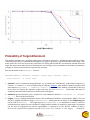
1
User Manual July 2015 An R package for parametric and non-‐parametric modeling and simula6on of pharmacokine6c and pharmacodynamic systems Table of Contents Introduc6on ...................................................................................................................................................3 Ci6ng Pmetrics ...............................................................................................................................................3 Disclaimer ......................................................................................................................................................3 System Requirements and Installa6on ...........................................................................................................3 What This Manual Is Not ................................................................................................................................5 GeHng Help and Updates ..............................................................................................................................5 Pmetrics Components ....................................................................................................................................5 Customizing Pmetrics Op6ons ........................................................................................................................6 General Workflow ..........................................................................................................................................7 Pmetrics Input Files ........................................................................................................................................8 Data .csv Files .........................................................................................................................................................8 Manipula6on of CSV files ........................................................................................................................................9 Model Files ...........................................................................................................................................................10 How to use R and Pmetrics ..........................................................................................................................18 Pmetrics Data Objects ..................................................................................................................................19 Making New Pmetrics Objects ......................................................................................................................24 Summarizing Pmetrics Objects .....................................................................................................................27 PMcov ............................................................................................................................................................27 PMfinal ...........................................................................................................................................................28 PMop ..............................................................................................................................................................31 PMpta ............................................................................................................................................................32 NPAG Runs ..................................................................................................................................................33 IT2B Runs .....................................................................................................................................................35 ERR Runs ......................................................................................................................................................35 Simulator Runs .............................................................................................................................................36 PloHng ........................................................................................................................................................42 Examples of Pmetrics plots .............................................................................................................................44 Probability of Target A^ainment ..................................................................................................................47 Model Diagnos6cs ........................................................................................................................................49 Internal Valida6on ................................................................................................................................................49 External Valida6on ...............................................................................................................................................52 Pmetrics Outputs .........................................................................................................................................52 Ancillary Func6ons .......................................................................................................................................53 References ...................................................................................................................................................53 User’s Guide 2 Introduction Thank you for your interest in Pmetrics! This guide provides instructions and examples to assist users of the Pmetrics R package, by the Laboratory of Applied Pharmacokinetics at the University of Southern California. Please see our website at http://www.lapk.org for more information. Here are some tips for using this guide. • Items that are hyperlinked can be selected to jump rapidly to relevant sections. • At the bottom of every page, the text “User’s Guide” can be selected to jump immediately to the table of contents. • Items in courier font correspond to R commands Citing Pmetrics Please help us maintain our funding to provide Pmetrics as a free research tool to the pharmacometric community. If you use Pmetrics in a publication, you can cite it as below. In R you can always type citation(“Pmetrics”) to get this same reference. Neely MN, van Guilder MG, Yamada WM, Schumitzky A, Jelliffe RW. Accurate Detection of Outliers and Subpopulations With Pmetrics, a Nonparametric and Parametric Pharmacometric Modeling and Simulation Package for R. Ther Drug Monit 2012; 34:467–476. Disclaimer You, the user, assume all responsibility for acting on the results obtained from Pmetrics. The USC Laboratory of Applied Pharmacokinetics, members and consultants to the Laboratory of Applied Pharmacokinetics, and the University of Southern California and its employees assume no liability whatsoever. Your use of the package constitutes your agreement to this provision. System Requirements and Installation Pmetrics and all required components will run under Mac (Unix), Windows, and Linux. There are three required software components which must be installed on your system in this order: 1. The statistical programming language and environment “R” 2. The Pmetrics package for R 3. gfortran or some other Fortran compiler A fourth, highly recommended, but optional component is Rstudio, a user-‐friendly wrapper for R. It can be installed any time after installing R (i.e. step 1 above). All components have versions for Mac, Windows, and Linux environments, and 32-‐ and 64-‐ bit processors. All are free of charge. R R is a free software environment for statistical computing and graphics, which can be obtained from http:// www.R-‐project.org/. Pmetrics is a library for R. Pmetrics If you are reading this manual, then you have likely visited our website at http://www.lapk.org, where you can select the software tab and download our products, including Pmetrics. User’s Guide 3 Pmetrics is distributed as a package source Zile archive (.tgz for Mac, .zip for Windows, .tar.gz for Linux). Do not o p e n t h e a r c h i v e . T o i n s t a l l P m e t r i c s f r o m t h e R c o n s o l e , u s e t h e c o m m a n d install.packages(file.choose()), and navigate when prompted to the folder in which you placed the Pmetrics package archive (.zip or .tgz) Zile. Pmetrics will need the following R packages for some functions: chron, Defaults, and R2HTML. However, you do not have to install these if you do not already have them in your R library. They should automatically be downloaded and installed when you use PMbuild() or the Zirst time you use a Pmetrics function that requires them, but if something goes awry (such as no internet connection or busy server) you can do this manually. Fortran In order to run Pmetrics, a Fortran compiler is required. After you have installed Pmetrics, the Zirst command to run is PMbuild() which will verify an installed fortran compiler on your system, or link you to the OS-‐speciZic page of our website with explicit instructions and a link to download and install gfortran on your system. Details of this procedure follow, but are not relevant if you already have a compiler installed. For Mac users the correct version of gfortran will be downloaded for your system (Mavericks 64-‐bit, Mountain Lion 64-‐bit, Lion 64-‐bit, Snow Leopard 64-‐ or 32-‐bit). You will also be provided a link to download and install Apple’s Xcode application if you do not already have it on your system. Xcode is required to run gfortran on Macs. As of version 4.3 for Lion, Xcode is available from the App store for free. For Snow Leopard, Xcode is on your installation disk. NOTE: For Xcode downloaded from the App store (Lion and later), you must additionally install the Command Line Tools available in the Xcode Preferences -‐> Downloads pane (Lion and Mountain Lion) or the Apple Developer website for Xcode 5 (Mavericks). Windows users need to pay special attention because the the “gcc” installer that provides necessary, common libraries for many programming languages does not by default include gfortran. When gcc is installed, be sure to choose the fortran option to include gfortran, as shown below. Click the expander bu>on Check this box Linux users have the easiest time, as gfortran comes with Linux. Rstudio A text editor that can link to R is useful for saving scripts. Both the Windows and Mac versions of R have rudimentary text editors that are stable and reliable. Numerous other free and paid editors can also do the job, and these can be located by searching the internet. We prefer Rstudio. User’s Guide 4 What This Manual Is Not We assume that the user has familiarity with population modeling and R, and thus this manual is not a tutorial for basic concepts and techniques in either domain. We have tried to make the R code simple, regular and well documented. A very good free online resource for learning the basics of R can be found at http:// www.statmethods.net/index.html. We recognize that initial use of a new software package can be complex, so please feel free to contact us at any time, preferably through the Pmetrics forum at http:/www.lapk.org or directly by email at [email protected]. This manual is also not intended to be a theoretical treatise on the algorithms used in IT2B or NPAG. For that the user is directed to our website at www.lapk.org. Getting Help and Updates There is an active LAPK forum available from our website at http://www.lapk.org with all kinds of useful tips and help with Pmetrics. Register (separately from your LAPK registration) and feel free to post! Within R, you can also use help(“command”) or ?command in the R console to see detailed help Ziles for any Pmetrics command. Many commands have examples included in this documentation and you can execute the examples with example(command). Note that, here, quotation marks are unnecessary around command. You can also type PMmanual() to launch this manual from within Pmetrics as well as a catalogue of all Pmetrics functions. Finally, PMnews() will display the Pmetrics changelog. Pmetrics will check for updates automatically every time you load it with library(Pmetrics). If an update is available, it will provide a brief message to inform you. You can then use PMupdate() to update Pmetrics from within R, without having to visit our website. You will be prompted for your LAPK user email address and password. When bugs arise in Pmetrics, you may see a start up message to inform you of the bug and a patch can be installed by the command PMpatch() if available. Note that patches must be reinstalled with this command every time you launch Pmetrics, until the bug is corrected in the next version. As of version 1.0.0 Pmetrics has graphical user interface (GUI) capability for many functions. Using PMcode(“function”) will launch the GUI in your default browser. While you are interacting with the GUI, R is “listening” and no other activity is possible. The GUI is designed to generate Pmetrics R code in response to your input in a friendly, intuitive environment. That code can be copied and pasted into your Pmetrics R script. You can also see live plot previews with the GUI. All this is made possible with the ‘shiny’ package for R. Currently, the following GUIs are available: PMcode(“NPrun”), PMcode(“ITrun”), PMcode(“plot”). More are coming! Pmetrics Components There are three main software programs that Pmetrics controls. • IT2B is the ITerative 2-‐stage Bayesian parametric population PK modeling program. It is generally used to estimate parameter ranges to pass to NPAG. It will estimate values for population model parameters under the assumption that the underlying distributions of those values are normal or transformed to normal. • NPAG is the Non-‐parametric Adaptive Grid software. It will create a non-‐parametric population model consisting of discrete support points, each with a set of estimates for all parameters in the model plus an associated probability (weight) of that set of estimates. There can be at most one point for each subject in the study population. There is no need for any assumption about the underlying distribution of model parameter values. • The simulator is a semi-‐parametric Monte Carlo simulation software program that can use the output of IT2B or NPAG to build randomly generated response proZiles (e.g. time-‐concentration curves) for a given population model, parameter estimates, and data input. Simulation from a non-‐parametric joint density model, i.e. NPAG output, is possible, with each point serving as the mean of a multivariate normal distribution, weighted according to the weight of the point. The covariance matrix of the entire set of support points is divided equally among the points for the purposes of simulation. User’s Guide 5 Pmetrics has groups of R functions named logically to run each of these programs and to extract the output. Again, these are extensively documented within R by using the help(command) or ?command syntax. • ITrun, ITparse, ERRrun • NPrun, NPparse • PMload, PMsave, PMreport • SIMrun, SIMparse For IT2B and NPAG, the “run” functions generate batch Ziles, which when executed, launch the software programs to do the analysis. ERRrun is a special implementation of IT2B designed to estimate the assay error polynomial coefZicients from the data, when they cannot be calculated from assay validation data (using makeErrorPoly()) supplied by the analytical laboratory. The batch Ziles contain all the information necessary to complete a run, tidy the output into a date/time stamped directory with meaningful subdirectories, extract the information, generate a report, and a saved Rdata Zile of parsed output which can be quickly and easily loaded into R. On Mac (Unix) systems, the batch Zile will automatically launch in a Terminal window. On Windows systems, the batch Zile must be launched manually. In both cases, the execution of the program to do the actual model parameter estimation is independent of R, so that the user is free to use R for other purposes. For the Simulator, the “SIMrun” function will execute the program directly within R. For all programs, the “parse” functions will extract the primary output from the program into meaningful R data objects. For IT2B and NPAG, this is done automatically at the end of a successful run, and the objects are saved in the output subdirectory as IT2Bout.Rdata or NPAGout.Rdata, respectively. For IT2B and NPAG, the “PMload” function can be used to load the either of the above .Rdata Ziles after a successful run. “PMsave” is the companion to PMload and can re-‐save modiZied objects to the .Rdata Zile. The “PMreport” function is automatically run at the end of a successful NPAG and IT2B run, and it will generate an HTML page with summaries of the run, as well as the .Rdata Ziles and other objects. The default browser will be automatically launched for viewing of the HTML report page. It will also generate a .tex Zile suitable for processing by a LATEX engine to generate a pdf report. See the Pmetrics Outputs section. Within Pmetrics there are also functions to manipulate data .csv Ziles and process and plot extracted data. • Manipulate data .csv Ziles: PMreadMatrix, PMcheck, PMwriteMatrix, PMmatrixRelTime, PMwrk2csv, NM2PM • Process data: makeAUC, makeCov, makeCycle, makeFinal, makeOP, makeNCA, makePTA, makeErrorPoly • Plot data: plot.PMcov, plot.PMcycle, plot.PMZinal, plot.PMmatrix, plot.PMop, plot.PMsim, plot.PMdiag, plot.PMpta • Model selection and diagnostics: PMcompare, plot.PMop (with residual option), makeNPDE, PMstep • Pmetrics function defaults: PMwriteDefaults Again, all functions have extensive help Ziles and examples which can be examined in R by using the help(command) or ?command syntax. Customizing Pmetrics Options You can change global options in Pmetrics setPMoptions(sep, dec) Currently you can change two options. sep will allow Pmetrics to read data Ziles whose Zield separators are semicolons and decimal separators are commas, e.g. setPMoptions(sep=”;”, dec=”,”). These options will persist from session to session until changed. getPMoptions() will return the current options. User’s Guide 6 General Workflow The general Pmetrics workZlow for IT2B and NPAG is shown in the following diagram. You supply these files; Pmetrics does the rest! Data .csv file u ITr n( n Pru ,) N Model .txt file () PreparaKon program InstrucKon file Engine program lo PM ad () sa PM () ve Output R is used to specify the working directory containing the data .csv and model .txt Ziles. Through the batch Zile generated by R, the preparation program is compiled and executed. The instruction Zile is generated automatically by the contents of the data and model Ziles, and by arguments to the NPrun(), ITrun() or ERRrun() commands. The batch Zile will then compile and execute the engine Zile according to the instructions, which will generate several output Ziles upon completion. Finally, the batch Zile will call the R script to generate the summary report and several data objects, including the IT2Bout.Rdata or NPAGout.Rdata Ziles which can be loaded into R subsequently using PMload(). Objects that are modiZied can be saved back to the .Rdata Ziles with PMsave(). Both input Ziles (data, model) are text Ziles which can be edited directly. User’s Guide 7 Pmetrics Input Files Data .csv Files Pmetrics accepts input as a spreadsheet “matrix” format. It is designed for input of multiple records in a concise way. Please keep the number of characters in the Vile name ≤ 8. Files are in comma-‐separated-‐values (.csv) format. Examples of programs that can save .csv Ziles are any text editor (e.g. TextEdit on Mac, Notepad on Windows) or spreadsheet program (e.g. Excel). Click on hyperlinked items to see an explanation. IMPORTANT: The order, capitalization and names of the header and the Zirst 12 columns are Zixed. All entries must be numeric, with the exception of ID and “.” for non-‐required placeholder entries. POPDATA DEC 11 #ID EVID TIME DUR GH GH GH GH GH GH GH GH 1423 1423 1423 1423 1423 1 0 0 0 4 1 0 0 1 1 0 0 0 0 0.5 1 2 0 3.5 5.12 24 0 0.1 1 2 2 0 . . . 0 0.5 . . 1 0 . . . DOSE ADDL II 400 . . . 150 150 . . 400 100 . . . . . . . . . . . -‐1 . . . . . . . . . . . . 12 . . . . INPUT OUT OUTEQ 1 . . . 1 1 . . 1 2 . . . . 1 1 1 . . 1 1 . . 1 1 2 . 0.42 0.46 2.47 . . 0.55 0.52 . . -‐99 0.38 1.6 C0 . 0.01 0.01 0.01 . 0.01 0.01 0.01 . . 0.01 0.01 0.05 C1 . 0.1 0.1 0.1 . 0.1 0.1 0.1 . . 0.1 0.1 0.2 C2 . 0 0 0 . 0 0 0 . . 0 0 -‐0.11 C3 COV… . 0 0 0 . 0 0 0 . . 0 0 0.002 POPDATA DEC_11 This is the Zixed header for the Zile and must be in the Zirst line. It identiZies the version. It is not the date of your data Zile. #ID This Zield must be preceded by the “#” symbol to conZirm that this is the header row. It can be numeric or character and identiZies each individual. All rows must contain an ID, and all records from one individual must be contiguous. Any subsequent row that begins with “#” will be ignored, which is helpful if you want to exclude data from the analysis, but preserve the integrity of the original dataset, or to add comment lines. IDs should be 11 characters or less but may be any alphanumeric combination. There can be at most 800 subjects per run. EVID This is the event ID Zield. It can be 0, 1, or 4. Every row must have an entry. 0 = observation 1 = input (e.g. dose) 2, 3 are currently unused 4 = reset, where all compartment values are set to 0 and the time counter is reset to 0. This is useful when an individual has multiple sampling episodes that are widely spaced in time with no new information gathered. This is a dose event, so dose information needs to be complete. TIME This is the elapsed time in decimal hours since the Zirst event. It is not currently clock time (e.g. 21:30), although this is planned. Every row must have an entry, and within a given ID, rows must be sorted chronologically, earliest to latest. User’s Guide 8 DUR This is the duration of an infusion in hours. If EVID=1, there must be an entry, otherwise it is ignored. For a bolus (i.e. an oral dose), set the value equal to 0. DOSE This is the dose amount. If EVID=1, there must be an entry, otherwise it is ignored. ADDL This speciZies the number of additional doses to give at interval II. It may be missing for dose events (EVID=1 or 4), in which case it is assumed to be 0. It is ignored for observation (EVID=0) events. Be sure to adjust the time entry for the subsequent row, if necessary, to account for the extra doses. If set to -‐1, the dose is assumed to be given under steady-‐state conditions. ADDL=-‐1 can only be used for the Zirst dose event for a given subject, or an EVID=4 event, as you cannot suddenly be at steady state in the middle of dosing record, unless all compartments/times are reset to 0 (as for an EVID=4 event). II This is the interdose interval and is only relevant if ADDL is not equal to 0, in which case it cannot be missing. If ADDL=0 or is missing, II is ignored. INPUT This deZines which input (i.e. drug) the DOSE corresponds to. Inputs are deZined in the model Zile. OUT This is the observation, or output value. If EVID=0, there must be an entry; if missing, this must be coded as -‐99. It will be ignored for any other EVID and therefore can be “.”. There can be at most 150 observations for a given subject. OUTEQ This is the output equation number that corresponds to the OUT value. Output equations are deZined in the model Zile. C0, C1, C2, C3 These are the coefZicients for the assay error polynomial for that observation. Each subject may have up to one set of coefZicients per output equation. If more than one set is detected for a given subject and output equation, the last set will be used. If there are no available coefZicients, these cells may be left blank or Zilled with “.” as a placeholder. COV... Any column after the assay error coefZicients is assumed to be a covariate, one column per covariate. Manipula6on of CSV files There are several functions in Pmetrics which are useful for either converting other formats into Pmetrics data Ziles, or checking Pmetrics data Ziles for errors and Zixing some of them automatically. PMreadMatrix(filename,...) This function simply reads "ilename and creates a PMmatrix object in memory which can be plotted (see ?plot.PMmatrix) or otherwise analyzed. PMcheck(PMmatrix|filename, model,...) This function will check a .csv Zile named "ilename or a PMmatrix data frame containing a previously loaded .csv Zile (the output of PMreadMatrix) for errors which would cause the analysis to fail. If a model Zile is provided, and the data Zile has no errors, it will also check the model Zile for errors. See ?PMcheck for details in R. PMwriteMatrix(data.frame, filename,...) This function writes an appropriate data.frame as a new .csv Zile. It will Zirst check the data.frame for errors via the PMcheck() function above, and writing will fail if errors are detected. This can be overridden with override=T. PMmatrixRelTime() This function converts dates and clock times of speciZied formats into relative times for use in the NPAG, IT2B and Simulator engines. See ?PMmatrixRelTime for details. PMwrk2csv() This function will convert old-‐style, single-‐drug USC*PACK .wrk formatted Ziles into Pmetrics data .csv Ziles. Details are available with ?PMwrk2csv in R. NM2PM() Although the structure of Pmetrics data Ziles are similar to NONMEM, there are some differences. This function attempts to automatically convert to Pmetrics format. It has been tested on several examples, but there are probably NONMEM Ziles which will cause it to crash. Running PMcheck() afterwards is a good idea. Details can be found with ?NM2PM in R. User’s Guide 9 Model Files Model Ziles for Pmetrics are ultimately Fortran text Ziles with a header version of TSMULT... As of Pmetrics version 0.30, we have adopted a very simple user format that Pmetrics will use to generate the Fortran code automatically for you. Version 0.4 additionally eliminates the previously separate instruction Zile. A model library is available on our website at http://www.lapk.org/pmetrics.php. Naming your model files. The default model Zile name is “model.txt,” but you can call them whatever you wish. However, please keep the number of characters in the model Vile name ≤ 8. When you use a model Zile in NPrun(), ITrun(), ERRrun(), or SIMrun(), Pmetrics will make a Fortran model Zile of the same name, temporarily renaming your Zile. At the end of the run, your original model Zile will be in the /inputs subfolder of the run folder, and the generated Fortran model Zile will be called “model.for” and moved to the /etc subfolder of the run folder. If your model is called “mymodel.txt”, then the Fortran Zile will be “mymodel.for”. You can still use appropriate Fortran model Ziles directly, but we suggest you keep the .for extension for all Fortran Ziles to avoid confusion with the new format. If you use a .for Zile as your model, you will have to specify its name explicitly in the NPrun(), ITrun, ERRrun(), or SIMrun() command, since the default model name again is “model.txt.” If you use a .for Zile directly, it will be in the /inputs subfolder of the run folder, not in /etc, since you did not use the simpler template as your model Zile. Structure of model files. The new model Zile is a text Zile with 11 blocks, each marked by "#" followed by a header tag. #PRImary variables #COVariates #SECcondary variables #BOLus inputs #INItial conditions #F (bioavailability) #LAG time #DIFferential equations #OUTputs #ERRor #EXTra For each header, only the capital letters are required for recognition by Pmetrics. The blocks can be in any order, and header names are case-‐insensitive (i.e. the capitalization here is just to show which letters are required). Fortran is also case-‐insensitive, so in variable names and expressions case is ignored. Details of each block are next, followed by a complete example. Important: Sometimes it is important to preserve spacing and formatting in Fortran code that you might insert into blocks, particularly the #EXTRA block. If you wish to do this, insert [format] and [/format] before and after any code that you wish to reproduce verbatim with spacing in the fortran model Zile. Comments: You can insert comments into your model text Zile by starting a line with a capital “C” followed by a space. These lines will be removed/ignored in the Zinal fortran code. Primary variables Primary variables are the model parameters that are to be estimated by Pmetrics or are designated as Zixed parameters with user speciZied values. It should be a list of variable names, one name to a line. Variable names should be 11 characters or fewer. Some variable names are reserved for use by Pmetrics and cannot be used as primary variable names. The number of primary variables must be between 2 and 32, with at most 30 random or 20 Vixed. On each row, following the variable name, include the range for the parameter that deZines the search space. These ranges behave slightly differently for NPAG, IT2B, and the simulator. User’s Guide 10 • For all engines, the format of the limits is min, max. A single value will Zix that parameter to the speciZied value. • For NPAG, the limits are absolute, i.e. the algorithm will not search outside this range. • For IT2B, the range deZines the Bayesian prior distribution of the parameter values for cycle 1. For each parameter, the mean of the Bayesian prior distribution is taken as the middle of the range, and the standard deviation is xsig*range (see IT2B runs). Adding an exclamation point (!) to a line will prevent that parameter from being assigned negative values. NPAG and the simulator will ignore the pluses as the ranges are absolute for these engines. • The simulator will ignore the ranges with the default value of NULL for the limits argument. If the simulator limits argument is set to NA, which will mean that these ranges will be used as the limits to truncate the simulation (see Simulator Runs). Example: #Pri KE, !0, 5 V, 0.01, 100 KA, 0, 5 KCP, 5 KPC, 0 , 5 Tlag1, 0, 2 IC3, 0, 10000 FA1, 0, 1 In this example, KE has a range of 0 to 5, which will be absolute for NPAG and the simulator (if limits=NA), but deCines the prior distribution for KE if using IT2B. The “!” limits KE to the positive real numbers for IT2B. KCP is Cixed to 5 regardless of the engine. Covariates Covariates are subject speciZic data, such as body weight, contained in the data .csv Zile. The covariate names, which are the column names in the data Zile, can be included here for use in secondary variable equations. The order should be the same as in the data Zile and although the names do not have to be the same, we strongly encourage you to make them the same to avoid confusion. Covariates are applied at each dose event. The Zirst dose event for each subject must have a value for every covariate in the data Zile. By default, missing covariate values for subsequent dose events are linearly interpolated between existing values, or carried forward if the Zirst value is the only non-‐missing entry. To suppress interpolation and carry forward the previous value in a piece-‐wise constant fashion, include an exclamation point (!) in any declaration line. Note that any covariate relationship to any parameter may be described as the user wishes by mathematical equations and Fortran code, allowing for exploration of complex, non-‐linear, time-‐dependent, and/or conditional relationships. Example: #Cov wt cyp IC(!) where IC will be piece-‐wise constant and the other two will be linearly interpolated for missing values. Secondary variables Secondary variables are those that are deZined by equations that are combinations of primary, covariates, and other secondary variables. If using other secondary variables, deZine them Zirst within this block. Equation syntax must be Fortran. It is permissible to have conditional statements, but because expressions in this block are User’s Guide 11 translated into variable declarations in Fortran, expressions other than of the form "X = function(Y)" must be preZixed by a "+" and contain only variables which have been previously deZined in the Primary, Covariate, or Secondary blocks. Example: #Sec CL = Ke * V * wt**0.75 +IF(cyp .GT. 1) CL = CL * cyp Bolus inputs By default, inputs with DUR (duration) of 0 in the data .csv Zile are "delivered" instantaneously to the model compartment equal to the input number, i.e. input 1 goes to compartment 1, input 2 goes to compartment 2, etc. This can be overridden with NBOLUS(input number) = compartment number. Example: #Bol NBCOMP(1) = 2 Ini6al condi6ons By default, all model compartments have zero amounts at time 0. This can be changed by specifying the compartment amount as X(.) = expression, where "." is the compartment number. Primary and secondary variables and covariates may be used in the expression, as can conditional statemtents in Fortran code. A "+" preZix is not necessary in this block for any statement, although if present, will be ignored. Example: #Ini X(2) = IC*V (i.e. IC is a covariate with the measured trough concentration prior to an observed dose) X(3) = IC3 (i.e. IC3 is a Zitted amount in this unobserved compartment) In the Zirst case, the initial condition for compartment 2 becomes the value of the IC covariate (deZined in #Covariate block) multiplied by the current estimate of V during each iteration. This is useful when a subject has been taking a drug as an outpatient, and comes in to the lab for PK sampling, with measurement of a concentration immediately prior to a witnessed dose, which is in turn followed by more sampling. In this case, IC or any other covariate can be set to the initial measured concentration, and if V is the volume of compartment 2, the initial condition (amount) in compartment 2 will now be set to the measured concentration of drug multiplied by the estimated volume for each iteration until convergence. In the second case, the initial condition for compartment 3 becomes another variable, IC3 deZined in the #Primary block, to Zit in the model, given the observed data. F (bioavailability) Specify the bioavailability term, if present. Use the form FA(.) = expression, where "." is the input number. Primary and secondary variables and covariates may be used in the expression, as can conditional statemtents in Fortran code. A "+" preZix is not necessary in this block for any statement, although if present, will be ignored. Example: #F FA(1) = FA1 Lag 6me Specify the lag term, if present, which is the delay after an absorbed dose before observed concentrations. Use the form TLAG(.) = expression, where "." is the input number. Primary and secondary variables and covariates may be User’s Guide 12 used in the expression, as can conditional statemtents in Fortran code. A "+" preZix is not necessary in this block for any statement, although if present, will be ignored. Example: #Lag TLAG(1) = Tlag1 Differen6al equa6ons Specify a model in terms of ordinary differential equations, in Fortran format. XP(.) is the notation for dX(.)/dt, where "." is the compartment number. X(.) is the amount in the compartment. There can be a maximum of 20 such equations. Example: #Dif XP(1) = -‐KA*X(1) XP(2) = RATEIV(1) + KA*X(1) -‐ (KE+KCP)*X(2) + KPC*X(3) XP(3) = KCP*X(2) -‐ KPC*X(3) RATEIV(1) is the notation to indicate an infusion of input 1 (typically drug 1). The duration of the infusion and total dose is deZined in the data .csv Zile. Up to 7 inputs are currently allowed. These can be used in the model Zile as RATEIV(1), RATEIV(2), etc. The compartments for receiving the inputs of oral (bolus) doses are deZined in the #Bolus block. Outputs Output equations, in Fortran format. Outputs are of the form Y(.) = expression, where "." is the output equation number. Primary and secondary variables and covariates may be used in the expression, as can conditional statemtents in Fortran code. A "+" preZix is not necessary in this block for any statement, although if present, will be ignored. There can be a maximum of 6 outputs. They are referred to as Y(1), Y(2), etc. Example: #Out Y(1) = X(2)/V Error This block contains all the information Pmetrics requires for the structure of the error model. In Pmetrics, each observation is weighted by 1/error2. There are two choices for the error term: 1. error = SD * gamma 2. error = (SD2 + lamda2)0.5 (Note that lambda is only available in NPAG currently). where SD is the standard deviation (SD) of each observation [obs], and gamma and lambda are terms to capture extra process noise related to the observation, including mis-‐speciZied dosing and observation times. SD is modeled by a polynomial equation with up to four terms: C0 + C1*[obs] + C2*[obs]2 + C3*[obs]3. The values for the coefZicients should ideally come from the analytic lab in the form of inter-‐run standard deviations or coefZicients of variation at standard concentrations. You can use the Pmetrics function makeErrorPoly() to choose the best set of coefZicients that Zit the data from the laboratory. Alternatively, if you have no information about the assay, you can use the Pmetrics function ERRrun() to estimate the coefZicients from the data. Finally, you can use a generic set of coefZicients. We recommend that as a start, C0 be set to half of the lowest concentration in the dataset and C1 be set to 0.15. C2 and C3 can be 0. In the multiplicative model, gamma is a scalar on SD. In general, well-‐designed and executed studies will have data with gamma values approaching 1. Poor quality, noisy data will result in gammas of 5 or more. Lambda is an additive model to capture process noise, rather than the multiplicative gamma model. User’s Guide 13 To specify the model in this block, the Zirst line needs to be either L=[number] or G=[number] for a lambda or gamma error model. The [number] term is the starting value for lambda or gamma. Good starting values for lambda are 1 times C0 for good quality data, 3 times C0 for medium, and 5 or 10 times C0 for poor quality. Note, that C0 should generally not be 0, as it represents machine noise (e.g. HPLC or mass spectrometer) that is always present. For gamma, good starting values are 1 for high-‐quality data, 3 for medium, and 5 or 10 for poor quality. If you include an exclamation point (!) in the declaration, then lambda or gamma will be Zixed and not estimated. Note that you can only Zix lambda currently to zero. The next line(s) contain the values for C0, C1, C2, and C3, separated by commas. There should be one line of coefZicients for each output equation. By default Pmetrics will use values for these coefZicients found in the data Zile. If none are present or if the model declaration line contains an exclamation point (!) the values here will be used. Example 1: estimated lambda, starting at 0.4, one output, use data Zile coefZicients but if missing, use 0.1,0.1,0,0 #Err L=0.4 0.1,0.1,0,0 Example 2: Zixed gamma of 2, two outputs, use data Zile coefZicients but if missing, use 0.1,0.1,0,0 for the Zirst output, but use 0.3, 0.1, 0, 0 for output 2 regardless of what is in the data Zile. #Err G=2! 0.1,0.1,0,0 0.3,0.1,0,0! Extra This block is for advanced Fortran programmers only. Occasionally, for very complex models, additional Fortran subroutines are required. They can be placed here. The code must specify complete Fortran subroutines which can be called from other blocks with appropriate call functions. As stated earlier, sometimes it is important to preserve spacing and formatting in Fortran code that you might insert into blocks, particularly the #EXTRA block. If you wish to do this, insert [format] and [/format] before and after any code that you wish to reproduce verbatim with spacing in the fortran model Zile. Reserved Names The following cannot be used as primary, covariate, or secondary variable names. They can be used in equations, however. Reserved Variable ndim Func6on in Pmetrics internal t time x array of compartment amounts xp array of Zirst derivative of compartment amounts rpar internal ipar internal User’s Guide 14 p array of primary parameters r input rates b input boluses npl internal numeqt output equation number ndrug input number nadd covariate number rateiv intravenous input for inputs when DUR>0 in data Ziles cv covariate values array n number of compartments nd internal ni internal nup internal nuic internal np number of primary parameters nbcomp bolus compartment array psym names of primary parameters fa biovailability tlag lag time tin internal tout internal User’s Guide 15 Complete Example Here is a complete example of a model Zile, as of Pmetrics version 0.40 and higher: #Pri KE, 0, 5 V0, 0.1, 100 KA, 0, 5 Tlag1, 0, 3 Notes: wt By omitting a #Diffeq block with ODEs, Pmetrics understands that you are specifying the model to be solved algebraically. In this case, at least KE and V must be in the Primary or Secondary variables. KA, KCP, and KPC are optional and specify absorption, and transfer to and from the central to a peripheral compartment, respectively. C this weight is in kg The comment line “C this weight is in kg” will be ignored. #Cov #Sec V = V0*wt #Lag TLAG(1) = Tlag1 #Out Y(1) = X(2)/V #Err L=0.4 0.1,0.1,0,0 User’s Guide 16 Brief Fortran Tutorial Much more detailed help is available from http://www.cs.mtu.edu/~shene/COURSES/cs201/NOTES/fortran.html. Arithme6c Operator Meaning + addition -‐ subtraction * multiplication / division ** exponentiation Rela6onal Operator Alterna6ve Operator Meaning < .LT. less than <= .LE. less than or equal > .GT. greater than >= .GE. greater than or equal == .EQ. equal /= .NE. not equal Selec6ve Execu6on Example IF (logical-‐expression) one-‐statement IF (T >= 100) CL = 10 IF (logical-‐expression) THEN statements END IF IF (T >= 100) THEN CL = 10 V = 10 END IF IF (logical-‐expression) THEN statements-‐1 ELSE statements-‐2 END IF IF (T >= 100) THEN CL = 10 ELSE CL = CL END IF User’s Guide 17 How to use R and Pmetrics SeHng up a Pmetrics project When beginning a new modeling project, it is convenient to use the command PMtree(“project name”). This command will set up a new directory in the current working directory named whatever you have included as the “project name”. For example, a directory called “DrugX” will be created by PMtree(“DrugX”). Beneath this directory, several subdirectories will be also created: Rscript, Runs, Sim, and src. The Rscript subdirectory will contain a skeleton R script to begin Pmetrics runs in the new project. The Runs subdirectory should contain all Ziles required for a run (described next) and it will also contain the resulting numerically ordered run directories created after each Pmetrics NPAG or IT2B run. The Sim subdirectory can contain any Ziles related to simulations, and the src subdirectory should contain original and manipulated source data Ziles. Of course, you are free to edit this directory tree structure as you please, or make your own entirely. GeHng the required files to run Pmetrics When you wish to execute a Pmetrics run, you must ensure that appropriate Pmetrics model .txt and data .csv Ziles are in the working directory, i.e. the Runs subdirectory of the project directory. R can be used to help prepare the data .csv Zile by importing and manipulating spreadsheets (e.g. read.csv()). The Pmetrics function PMcheck() can be used to check a .csv Zile or an R dataframe that is to be saved as a Pmetrics data .csv Zile for errors. It can also check a model Zile for errors in the context of a dataZile, e.g. covariates that do not match. PMcheck(...,fix=T) attempts to automatically rid data Ziles of errors. The function PMwriteMatrix() can be used to write the R data object in the correct format for use by IT2B, NPAG, or the Simulator. You can also download sample data and scripts from the Pmetrics downloads section of our website. Edit prior versions of model Ziles to make new model Ziles. Using scripts to control Pmetrics As you will see in the skeleton R script made by PMtree() and placed in the Rscript subdirectory, if this is a Zirst-‐ time run, the R commands to run IT2B or NPAG are as follows. Recall that the “#” character is a comment character. library(Pmetrics) #Run 1 - add your run description here setwd(“working directory”) NPrun() #for NPAG or ITrun() for IT2B The Zirst line will load the Pmetrics library of functions. The second line sets the working directory to the speciZied path. The third line generates the batch Zile to run NPAG or IT2B and saves it to the working directory. NOTE: On Mac systems, the batch Zile will be automatically launched in a Terminal window. On Windows systems, the batch Zile must be launched manually by double clicking the npscript.bat or itscript.bat Zile in the working directory. ITrun() and NPrun() both return the full path of the output directory to the clipboard. By default, runs are placed in folders numbered sequentially, beginning with “1”. Now the output of IT2B or NPAG needs to be loaded into R, so the next command does this. PMload(run_number) Details of these commands and what is loaded are described in the R documentation (?PMload) and in the following section. The run_number should be included within the parentheses to be appended to the names of loaded R objects, allowing for comparison between runs, e.g. PMload(1). Finally, at this point other Pmetrics commands can be added to the script to process the data, such as the following. User’s Guide 18 plot(final.1) plot(cycle.1) plot(op.1,type=”pop”) or plot(op.1$pop1) plot(op.1) #default is to plot posterior predictions for output 1 plot(op.1,type=”pop”,resid=T) Of course, the full power of R can be used in scripts to analyze data, but these simple statements serve as examples. If you do not use the PMtree() structure, we suggest that the R script for a particular project be saved into a folder called “Rscript” or some other meaningful name in the working directory. Folders are not be moved by the batch Zile. Within the script, number runs sequentially and use comments liberally to distinguish runs, as shown below. library(Pmetrics) #Run 1 - Ka, Kel, V, all subjects setwd(“working directory”) NPrun() #assumes model=”model.txt” and data=”data.csv” PMload(1) ... Remember in R that the command example(function) will provide examples for the speciZied function. Most Pmetrics functions have examples. Pmetrics Data Objects After a successful IT2B or NPAG run, an R dataZile is saved in the output subdirectory of the newly created numerically ordered folder in the working directory. After IT2B, this Zile is called “IT2Bout.Rdata”, and after NPAG it is called “NPAGout.Rdata”. As mentioned in the previous section, these data Ziles can be loaded by ensuring that the Runs folder is set as the working directory, and then using the Pmetrics commands PMload(run_num). There are several Pmetrics data objects contained within the Rdata Ziles which are loaded with PMload(), making these objects available for plotting and other analysis. Objects loaded by PMload(run_num) Objects op (class: PMop, list) Variables Comments $id Subject identiZication $time Observation time in relative decimal hours $obs Observation $pred Predicted value $pred.type Type of prediction, i.e. based on the population parameter values or Bayesian posterior parameter values $icen Median (default) or mean of the parameter distributions used to calculate the predicted values. $outeq User’s Guide 19 Objects Zinal (class: PMZinal, list) Variables Comments $block Dosing block, usually 1 unless data Zile contains EVID=4 dose reset events, in which case each such reset within a given ID will increment the dosing block by 1 for that ID $obsSD Calculated standard deviation (error) of the observation based on the assay error polynomial $d Difference between pred and obs $ds Squared difference between pred and obs $wd $d, weighted by the $obsSD $wds $ds, weighted by the $obsSD $popPoints (NPAG only) Data.frame of the Zinal cycle joint population density of grid points with column names equal to the name of each random parameter plus $prob for the associated probability of that point $popMean The Zinal cycle mean for each random parameter distribution $popSD The Zinal cycle standard deviation for each random parameter distribution $popCV The Zinal cycle coefZicient of variation for each random parameter distribution $popVar The Zinal cycle variance for each random parameter distribution $popCov The Zinal cycle covariance matrix for each random parameter distribution $popCor The Zinal cycle correlation matrix for each random parameter distribution $popMedian The Zinal cycle median for each random parameter distribution $gridpts (NPAG only) The initial number of support points $ab Matrix of boundaries for random parameter values. For NPAG, this is speciZied by the user prior to the run; for IT2B, it is calculated as a user speciZied multiple of the SD for the parameter value distribution User’s Guide 20 Objects cycle (class: PMcycle, list) cov (class: PMcov, data.frame) Variables Comments $postPoints (NPAG only) Data frame of the Bayesian posterior parameter points for each of the Zirst 100 subjects, with the following columns: id: subject ID point: point number for that subject parameters: parameters in the model prob: probability of each point in the posterior for each patient $names Vector of names of the random parameters $ll Matrix of cycle number and -‐2*Log-‐likelihood at each cycle $gamlam A matrix of cycle number and gamma or lambda at each cycle (see item #16 under NPAG Runs below for a discussion of gamma and lambda) $mean A matrix of cycle number and the mean of each random parameter at each cycle, normalized to initial mean $sd A matrix of cycle number and the standard deviation of each random parameter at each cycle, normalized to initial standard deviation $median A matrix of cycle number and the median of each random parameter at each cycle, normalized to initial standard deviation $aic A matrix of cycle number and Akaike Information Criterion at each cycle $bic A matrix of cycle number and Bayesian (Schwartz) Information Criterion at each cycle $id Subject identiZication $time Time for each covariate entry covariates... Covariate values for each subject at each time, extracted from the raw data Zile User’s Guide 21 Objects pop (class: PMpop, data.frame) Variables Comments parameters... Mean, median, or mode of Bayesian posterior distribution for each random parameter in the model. Mode summaries are available for NPAG output only, and the default is median. Values are recycled for each row within a given subject, with the number of rows driven by the number of covariate entries $icen Median (default) or mean of the covariates and parameter value distributions. $id Subject identiZication $time Time of each prediction at a frequency speciZied in the NPrun() command, with a default of 12 minutes. $icen Median (default) or mean of the parameter distributions used to calculate the predicted values. $pred Population prior (PMpop) or Bayesian posterior (PMpost) predictions for each output equation $outeq Output equation for each prediction $block Same as for PMop objects above post (class: PMpost, data.frame) NPAG only NPdata (class: NPAG, list) ITdata (class: IT2B, list Raw data used to make the above objects. Please use ?NPparse or ?ITparse in R for discussion of the data contained in these objects mdata (class: PMmatrix, data.frame) See Pmetrics Input Your original raw data Zile. Files. NPDE (class: PMnpde, list) Use the command str(NPDE.x) in R, where x is the run number This object will only be present if you have run makeNPDE() after a run is completed. This object contains the information to perform graphical and numerical analysis of normalized prediction distribution errors. It is a method of internal model validation. User’s Guide 22 Objects sim (class: PMsim, list) Variables Comments $obs A data frame with $id, $time, $out, $outeq columns containing simulated observations at each time and output equation number in the template data Zile. If simulations from multiple template subjects have been combined (see Simulator Runs), then $id will be of the form x.y, where x is the simulation number, and y is the template number. $amt A data frame with $id, $time, $out, $comp columns containing simulated amounts in each compartment. $parValues A data frame with $id, ... columns containing the parameter value sets for each simulated subject with “...” signifying the columns named according to the names of the random parameters in the model $totalSets The total number of simulated sets of parameters, which may be greater than the requested number if limits were speciZied in the simulation (see Simulator Runs). $totalMeans The means of the parameter values in the total simulated sets which can be used as a check of the adequacy of the simulation to reproduce the requested mean values when limits were applied. The Zinal truncated set will likely not have the requested mean values. $totalCov The covariances of the parameter values in the total simulated sets which can be used as a check of the adequacy of the simulation to reproduce the requested covariance values when limits were applied. The Zinal truncated set will likely not have the requested covariance values. This object will only be present if you have run makeNPDE() after a run is completed. Since R is an object oriented language, to access the observations in a PMop object, for example, use the following syntax: op$post1$obs. Note that you will place an integer corresponding to the run number within the parentheses of the loading functions, e.g. PMload(1), which will sufZix all the above objects with that integer, e.g. op.1, Zinal.1, NPdata.1. This allows several models to be loaded into R simultaneously, each with a unique sufZix, and which can be compared with the PMcompare() command (see Model Diagnostics below). User’s Guide 23 Making New Pmetrics Objects Once you have loaded the raw (NPdata or ITdata and mdata) or processed (op, Vinal, cycle, pop, post) data objects described above with PMload(run_num), should you wish to remake the processed objects with parameters other than the defaults, you can easily do so with the make family of commands. For example, the default for PMop observed vs. predicted objects is to use the prediction based on the median of the population or posterior distribution. If you wish to use the mean of the distribution, remake the PMop object using makeOP(). If you wish to see all the cycle information in a PMcycle object, not omitting the Zirst 10% of cycles by default, remake it using makeCycle(). For all of the following commands, the data input is either NPdata or ITdata, with additional function arguments speciZic to each command. Accessing the help for each function in R will provide further details on the arguments, defaults and output of each command. Command Description R help makeAUC Make a data.frame of class PMauc containing subject ID ?makeAUC and AUC from a variety of inputs including objects of PMop, PMsim, PMpop, PMpost or a suitable data.frame makeCov Generate a data.frame of class PMcov with subject-‐ ?makeCov speciZic covariates extracted from the data .csv Zile. This object can be plotted and used to test for covariates which are signiZicantly associated with model parameters. makeCycle Create a PMcycle object described in the previous section. ?makeCycle makeFinal Create a PMZinal object described in the previous section. ?makeFinal makeOP Create a PMop object described in the previous section. ?makeOP User’s Guide 24 Command makeNCA Description Create a data.frame (class PMnca) with the output of a non-‐compartmental analysis using PMmatrix or PMpost data objects as input. The PMnca object contains several columns. • • • • • • • • • • • • • • • makeErrorPoly R help ?makeNCA id: Subject identiZication auc: Area under the time-‐observation curve, using the trapezoidal approximation, from time 0 until the second dose, or if only one dose, until the last observation aumc: Area under the Zirst moment curve k: Slope by least-‐squares linear regression of the Zinal 6 log-‐transformed observations vs. time auclast: Area under the curve from the time of the last observation to inZinity, calculated as [Final obs]/ k aumclast: Area under the Zirst moment curve from the time of the last observation to inZinity aucinf: Area under the curve from time 0 to inZinity, caluculated as auc + auclast aumcinf: Area under the Zirst moment curve from time 0 to inZinity mrt: Mean residence time, calculated as 1/k cmax: Maximum predicted concentration after the Zirst dose tmax: Time to cmax cl: Clearance, calculated as dose/aucinf vdss: Volume of distribution at steady state, calculated as cl*mrt thalf: Half life of elimination, calculated as ln(2)/k dose: First dose amount for each subject This function plots Zirst, second, and third order ?makeErrorPoly polynomial functions Zitted to pairs of observations and associated standard deviations for a given output assay. In this way, the standard deviation associated with any observation may be calculated and used to appropriately weight that observation in the model building process. Observations are weighted by the reciprocal of the variance, or squared standard deviation. Output of the function is a plot of the measured observations and Zitted polynomial curves and a list with the Zirst, second, and third order coefZicients. User’s Guide 25 Command makePTA Description R help This function performs a Probability of Target ?makePTA Attainment analysis for a set of simulated doses and time-‐concentration proZiles. Targets (e.g. Minimum Inhibitory Concentrations), the type of target attainment (i.e. %time above target, Cmax:target , AUC:target, Cmin:target, or Cx:target, where x is any time point), and the success threshold (e.g. %time > 0.7 or Cmax:target > 10) can all be speciZied. Output is a list (class PMpta) with two objects • Results: A data frame with the following columns: simnum is the number of the simulation; id is the simulated proZile number within each simulation; target is the speciZied target; and pdi is the target pharmacodynamic index, e.g. time > target, auc:target, etc. • Outcome: A data frame summarizing the results with the following columns: simnum and target are as for results; prop.success column has the proportion with a pdi > success, as speciZied in the function call; pdi.mean and pdi.sd columns have the mean and standard deviation of the target pharmacodynamic index (e.g. proportion end-‐start above target, ratio of Cmax to target) for each simulation and target. If targets was speciZied via makePTAtarget to be a sampled distribution, then the target column will be missing from the outcome table. PMpta objects can be summarized with summary(x) and plotted with plot(x) . makePop makePost (NPAG only) These functions create data.frames of class PMpop and ?makePop PMpost, respectively. ?makePost The PMpop or PMpost object contains several columns as described in the previous section. User’s Guide 26 Command makeNPDE Description R help This function is a Pmetrics wrapper to the autoNPDE ?makeNPDE function in the NPDE package of Comets et al ?NPDE::autoNPDE (automatically loaded with Pmetrics) that will generate ?NPDE::NpdeObject an PMnpde object which is a list of NpdeObjects (one for each output equation). NpdeObjects contain normalized prediction distribution errors. For a given NPAG or IT2B run number and output equation, this function will iterate through the data .csv Zile, using each subject as a template to simulate nsim new individuals from the population prior. It is HIGHLY recommended to use the default value of 1000 for nsim for the most valid calculation of NPDE. More than this could take a long time to execute. The mean population values will be used for each parameter and the covariance matrix. Errors may arise if extreme or negative concentrations are simulated from excessively large covariance matrices. Because considerable time may be necessary to make the NpdeObject, it will be added as an NPDE item to the NPAGout.Rdata or IT2Bout.Rdata objects so that it will be loaded the next time PMload() is run. Additionally, the combined simulations for all the subjects in the dataset will be saved as a sim item in the NPAGout.Rdata or IT2B.Rdata objects. Summarizing Pmetrics Objects There are summary commands available for several Pmetrics objects, as detailed below. All objects can be summarized by the R command summary(x), where x is the object you wish to summarize. PMcov summary(x, icen = "median") ?summary.PMcov Summarize a PMcov object by creating a data frame with each subject’s covariate values and Bayesian posterior parameter values, summarized according to icen. Default is “median” covariate values and Bayesian posterior parameter values, but could be “mean”. Example data(PMex1) summary(cov.1, “mean”) id time wt africa age gender height Ka User’s Guide 27 Ke V Tlag1 1 60 46.7 1 21 1 160 0.440395 0.024616 66.3924 0.554941 2 60 66.5 1 30 1 174 0.7405 0.0398 119.476 0.0269964 3 60 46.7 1 24 0 164 0.899944 0.0431027 108.649 2.09592 4 60 50.8 1 25 1 165 0.897547 0.0564307 119.819 0.688301 5 60 65.8 1 22 1 181 0.105318 0.0675052 113.344 0.0186971 6 60 65 1 23 1 177 0.895218 0.0348829 71.8626 1.99784 7 60 51.7 1 27 0 161 0.215198 0.0832836 35.2243 1.79653 8 60 51.2 1 22 1 163 0.895481 0.0348882 71.847 1.99849 9 60 55 1 23 1 174 0.789913 0.0439419 101.783 0.879688 10 60 52.1 1 32 1 163 0.655786 0.0615878 61.6927 0.801376 11 60 56.5 1 34 1 165 0.583223 0.068323 73.1082 1.33855 12 60 47.9 1 54 0 160 0.470306 0.0306883 91.8595 1.02535 13 60 60.5 1 24 1 180 0.215198 0.0832837 35.2243 1.79559 14 60 59.2 1 26 1 174 0.579989 0.0439032 117.837 0.336257 15 60 43 1 19 0 150 0.795628 0.034209 72.2038 1.05869 16 60 64.4 1 25 1 173 0.752955 0.0352986 89.6704 0.687976 17 60 54.8 1 23 1 170 0.891255 0.0734126 63.3196 1.17994 18 60 44.3 1 20 0 164 0.894613 0.023192 75.9273 1.76035 19 60 50 1 36 1 168 0.662597 0.0621169 30.9852 1.92418 20 60 59 1 31 1 170 0.215198 0.0832837 35.2243 1.79584 PMfinal summary(x, lower = 0.025, upper = 0.975) ?summary.PMfinal For NPAG runs, this function will generate a data frame with weighted medians as central tendencies of the population points with an upper -‐ lower (default 95%) conZidence interval (95% CI) around the median, and the median absolute weighted deviation (MAWD) from the median as a measure of the variance, with its 95% CI. These estimates correspond to weighted mean, 95% CI of the mean, variance, and 95% CI of the variance, respectively, for a sample from a normal distribution. To estimate these non-‐parametric summaries, the function uses a Monte Carlo simulation approach, creating 1000 x npoint samples with replacement from the weighted marginal distribution of each parameter, where npoint is the number of support points in the model. As an example, if there are 100 support points, npoint = 100, and for Ka, there will be 1000 sets of 100 samples drawn from the weighted marginal distribution of the values for Ka. For each of the 1,000 sets of npoint values, the median and MAWD are calculated, with MAWD equal to the median absolute difference between each point and the median of that set. The output is npoint estimates of the weighted median and npoint estimates of the MAWD for each parameter, from which the median, 2.5th, and 97.5th percentiles can be found as point estimates and 95% conZidence interval limits, respectively, of both the weighted median and MAWD. For IT2B runs, the function will return the mean and variance of each parameter, and the standard errors of these terms, using SE (mean) = SD/sqrt(nsub) and SE (var) = var * sqrt(2/(nsub-‐1)). User’s Guide 28 Example data(PMex1) summary(final.1) par type quantile value Ka WtMed 0.025 5.19E-01 Ka WtMed 0.5 7.05E-01 Ka WtMed 0.975 8.48E-01 Ka MAWD 0.025 5.19E-02 Ka MAWD 0.5 1.59E-01 Ka MAWD 0.975 3.07E-01 Ke WtMed 0.025 3.51E-02 Ke WtMed 0.5 4.39E-02 Ke WtMed 0.975 6.48E-02 Ke MAWD 0.025 4.94E-03 Ke MAWD 0.5 1.48E-02 Ke MAWD 0.975 2.18E-02 V WtMed 0.025 6.47E+01 V WtMed 0.5 7.25E+01 V WtMed 0.975 1.00E+02 V MAWD 0.025 6.25E+00 V MAWD 0.5 2.07E+01 V MAWD 0.975 3.73E+01 Tlag1 WtMed 0.025 6.88E-01 Tlag1 WtMed 0.5 1.11E+00 Tlag1 WtMed 0.975 1.79E+00 Tlag1 MAWD 0.025 1.70E-01 Tlag1 MAWD 0.5 5.02E-01 Tlag1 MAWD 0.975 7.89E-01 In this example, the weighted median for Tlag1 is 1.11, with a 95% CI around the weighted median of 0.0688 to 1.79. The median absolute weighted difference (MAWD) is 0.502 with a 95% CI of 0.17 to 0.789. PMmatrix summary(x, formula, FUN, ..., include, exclude) ?summary.PMfinal User’s Guide 29 This function will summarize a Pmetrics data Zile, which is of class PMmatrix when loaded by PMreadMatrix() or PMload(). The simplest is to summarize just the object. For example: data(PMex1) summary(mdata.1) Number of subjects: 20 Number of inputs: 1 Number of outputs: 1 Total number of observations (outeq 1): 139, with 0 (0.000%) missing Number of covariates: 5 THE FOLLOWING ARE MEAN (SD), MIN TO MAX --------------------------------------INPUTS Number of doses per subject (input 1): 6.000 (0.000), 6.000 to 6.000 Dose per subject (input 1): 585.000 (45.189), 450.000 to 600.000 OUTPUTS Number of obs per subject (outeq 1): 6.950 (0.224), 6.000 to 7.000 Observation per subject (outeq 1): 7.241 (3.799), 1.860 to 20.150 COVARIATES wt: 54.538 (7.173), 43.000 to 66.500 africa: 1.000 (0.000), 1.000 to 1.000 age: 27.035 (7.717), 19.000 to 54.000 gender: 0.749 (0.434), 0.000 to 1.000 height: 167.792 (7.562), 150.000 to 181.000 --------------------------------------Note: See help(summary.PMmatrix) for accessing specific items by name. An object of class summary.PMmatrix is also returned. This object is a list with the following items. • • • • • • • • • • • • nsub The number of subjects. ndrug The number of drug inputs. numeqt The number of output equations. nobsXouteq The number of observations by output equation. missObsXouteq The number of missing observations by output equation. ncov The number of covariates. covnames The covariate names. ndoseXid The number of doses per input per subject. nobsXid The number of observations per output equation per subject. doseXid The doses per input per subject. obsXid The observations per output per subject. formula The results of including a formula. To include a formula, use standard R notation for the formula and specify the aggregating function with FUN. Example To calculate average dose in mg/kg per subject... summ <- summary(mdata.1, formula = I(dose/wt)~id, FUN=”mean”) summ$formula id I(dose/wt) User’s Guide 30 1 12.847966 2 9.022556 3 12.847966 4 11.811024 5 9.118541 6 9.230769 7 11.605416 8 11.71875 9 10.909091 10 11.516315 11 10.619469 12 12.526096 13 9.917355 14 10.135135 15 10.465116 16 9.31677 17 10.948905 18 10.158014 19 12 20 10.169492 mean(summ$formula[,2]) #choose the second column [1] 10.84424 PMop summary(x, digits = max(3, getOption("digits") - 3), pred.type = "post", icen = "median", outeq = 1) ?summary.PMop This will summarize a PMop object that contains observations, predictions and errors. You can specify the number of digits, predictions based on posterior or population predictions, or based on mean or median parameter distributions, for any output equation. Example data(PMex1) summary(op.1) #summarize based on medians of Bayesian posterior parameter values Time Obs Pred User’s Guide 31 Min 120.0000 1.8600 1.9648 25% 121.0250 4.4950 4.5019 Median 126.0000 6.5600 6.5996 75% 132.0000 8.8850 8.9355 Max 144.9800 20.1500 19.8025 Mean 127.6899 7.2407 7.0689 7.8600 3.7992 3.6420 SD Mean prediction error: -0.1718 Mean weighted prediction error (bias): -0.103 (P=0.9718 different than 0) Mean squared prediction error: 0.795 Root mean squared error (RMSE): 0.8916 Percent root mean squared error (%RMSE): 12.3141 Mean weighed squared prediction error: 0.992 Bias-adjusted mean squared prediction error: 0.7655 Bias-adjusted mean weighted squared prediction error (imprecision): 0.9813 This function also returns a list with three items. The Zirst item of the list is a data frame with the minimum, Zirst quartile, median, third quartile, maximum, mean and standard deviation for times, observations and predictions in x. The second is a data frame of one row whose columns contain the mean prediction error, the mean weighted prediction error (bias), the mean squared prediction error, root mean sqaured error (RMSE), percent root mean squared error ( squared prediction error, the bias-‐adjusted mean squared prediction error, and the bias-‐ adjusted mean weighted squared prediction error (imprecision). The third is itself a list of 6 items related to the weighted prediction bias, which are the mean, the standard error of the mean, the 95% conZidence interval, the t-‐statistic, the degrees of freedom, and the p-‐value (compared to a bias of 0). In the example above, the p-‐value is 0.9718. PMpta summary(x, ci = 0.95, ...) ?summary.PMpta This function returns a list with two named objects: pta (probability of target attainment) and pdi (pharmacodynamic index). pta A data frame with the following columns: simnum, target, prop.success, pdi.mean, and pdi.sd simnum is the number of the simulation; target is the speciZied target; success has the proportion with a ratio > prop.success; pdi.mean and pdi.sd are the mean and standard deviation of the pharmacodynamic index (e.g. AUC/MIC) for each simulation and target. pdi A data frame with the following columns: target, simnum, lowerCI, median, upperCI. target and simnum are as above. lowerCI, median, and upperCI are the lower limit, median, and upper limit of the conZidence interval for the pdi whose width is speciZied by ci. User’s Guide 32 NPAG Runs Here we provide details of the arguments available to the NPrun() command. You must have a data and model Zile in your working directory. In the R syntax below, any argument with a value has a default equal to that value and if you wish to use that default, you do not have to specify the argument in your function call to NPrun(). NPrun(model = "model.txt", data = "data.csv", run, include, exclude, ode = -4, tol = 0.01, salt, cycles = 100, indpts, icen = "median", aucint, idelta = 12, prior, overwrite = F, nocheck = F, parallel = NA) 1. model Name of a suitable model Zile template in the working directory or an existing (previous) run number corresponding to a folder in the current working directory that used the same model Zile as will be used in the current run. If this is supplied, then the model Zile will be copied into the current working directory for convenience. If not supplied, the default is “model.txt”. This Zile will be converted to a fortran model Zile. If it is detected to already be a fortran Zile, then the analysis will proceed without any further Zile conversion. Examples: NPrun(), NPrun(model=“model2.txt”), NPrun(model=2). The Zirst example uses all the default options. The second example uses the defaults except for the model Zile. The third example uses the same model as that used in Run 2, but defaults otherwise. 2. data Name of a suitable data Zile or an existing (previous) run number corresponding to a folder in the current working directory that used the same data Zile as will be used in the current run. If this is supplied, then previously made '.ZMQ' Ziles will be copied into the current working directory, bypassing the need to re-‐ convert the .csv Zile and speeding up the run. Examples: NPrun(data=“data2.csv”), NPrun(data=2). The Zirst example uses the defaults except for the data Zile. The second example uses the same data Zile as that used in Run 2, but defaults otherwise. 3. run Specify the run number of the output folder. Default if missing is the next available number. Examples: NPrun(), NPrun(run=2). The Zirst example uses all the default options and the run number will be automatically assigned to “3” if runs 1 and 2 already exist. The second example uses the defaults except for the run number. If runs 1 and 3 exist and you have deleted run 2 because you wish to re-‐run it, then this syntax will place the output in a folder labeled “2”. If you haven’t already deleted the old run folder, you can set overwrite #15 below, to True. 4. include Vector of subject id values in the data Zile to include in the analysis. The default (missing) is all. Examples: NPrun(include=c(1:3, 5)). Include only subjects with ID numbers of 1, 2, 3 and 5. 5. exclude Vector of subject id values in the data Zile to exclude in the analysis. The default (missing) is none. Be careful if you include and exclude in the same run as you may have conZlicting statements. Examples: NPrun(exclude=c(1:3, 5)). Exclude subjects with ID numbers of 1, 2, 3 and 5. 6. ode Ordinary Differential Equation solver log10 tolerance or stiffness. Default is -‐4, i.e. 0.0001. Higher values will result in faster runs, but parameter estimates may not be as accurate. It is ignored if the model does not use differential equations. Examples: NPrun(ode=-3). Do the run with a stiffness of 0.001, which will be faster than the default but perhaps less accurate. 7. tol Tolerance for convergence of NPAG. Smaller numbers make it harder to converge. Default value is 0.01. Examples: NPrun(tol=0.001). Do the run with a tolerance of 0.001, which will be slower than the default but perhaps more accurate. 8. salt Vector of salt fractions for each ndrug, default is 1 for each drug. This is not the same as bioavailability. Examples: NPrun(salt=c(1,0.9)). This sets the salt fraction for the Zirst drug to 1 and for the second drug to 0.9. 9. cycles Maximum number of NPAG cycles to run. Default is 100, but the value can be 0 or greater. If you enter an integer greater than 0, the engine will terminate at convergence or the number of cycles you specify, whichever comes Zirst. Early in model exploration values of 10 to 100 can be useful, with larger values later in model development. In order to facilitate model comparison, however, we recommend using the same cycle limit for all early models, e.g. 100, rather than choosing 10 for one and 100 for another. If you enter 0, this is the way to test the predictive power of a model on an independent data set and a non-‐uniform prior must be User’s Guide 33 speciZied. This means that the engine will only calculate the individual Bayesian posteriors for the new subjects, using the population joint density from a previous run as a Bayesian prior. Examples: NPrun(cycles=1000), NPrun(data=”newdata.csv”,cycles=0,prior=NPdata.1). The Zirst example will allow NPAG to run 1000 cycles before terminating. The second example calculates Bayesian posteriors only (i.e. NPAG is not cycling) using the default model Zile and some new data. Note by specifying a prior, which is required with 0 cycles, the grid points are distributed in a non-‐uniform manner corresponding to the prior distribution in NPdata.1 (the output of Run 1). This means that the indpts argument will be ignored. See also prior #14 below. 10. indpts Index of starting grid point number. Default is missing, which allows NPAG to choose depending on the number of random parameters: 1 or 2 parameters = index of 1; 3 = 3; 4 = 4, 5 = 6, 6 or more is 10+number of multiples for each parameter greater than 5, e.g. 6 = 101; 7 = 102, up to 108 for 13 or more parameters. This number corresponds to the number of grid (support) points which will initially Zill the model parameter space. The larger the number of random parameters to be estimated, the more points are required. The more you choose, the slower the run will be, but results may improve. It is reasonable to choose fewer points early in model exploration and increase in later phases or if poor model Zits or lack of convergence are noted. Indices of 1 to 6 correspond respectively to 2129, 5003, 10007, 20011, 40009, and 80021 points. 101 will choose 80021 points plus one additional multiple of 80021 points. Examples: NPrun(indpts=102). This will allow NPAG to start with 80021 + 2*80021 = 240063 points. The unusual numbers are from early development of NPAG where primes were thought to be important. 11. icen Summary of parameter distributions to be used to calculate predictions. Default is "median", and other choices are "mean" or "mode". Examples: NPrun(icen=”mean”). This example will use the means of the parameter distributions (rather than the medians) to calculate predictions. 12. aucint Interval for AUC calculations. Default is 24 hours if the number of intervals is not greater than 48; otherwise it defaults to the interval which allows for <= 48 intervals. Examples: NPrun(aucint=12). This example will use an interval of 12 hours for AUC estimations directly by NPAG. Note that the command makeAUC() can be used to calculate AUCs of any interval from the output. 13. idelta Interval in minutes for predictions at times other than observations. Default is 12 minutes, which in general, for most models provides sufZicient granularity. Smaller values can result in very large Ziles for big populations. Examples: NPrun(idelta=60). This generates predictions every 60 minutes. 14. prior Name of a suitable NPAG output object from a prior run loaded with PMload(), i.e. the NPdata object. A prior may be speciZied if the user wishes to start from a non-‐uniform prior distribution for the NPAG run. The default value is -‐99, which translates in NPAG to a uniform prior distribution. An alternative is to include a DEN0001 Zile from the prior NPAG run in the working directory of the new run, and specify this as the value for prior, e.g. prior = 'DEN0001'. Examples: NPrun(data=2,model=2,prior=NPdata.2). This example will use the model, data, and population density Ziles from Run 2 to continue for another 100 cycles. This is a useful way to continue a previous run that has not converged. See also cycles #9 above for a discussion and example of specifying a prior simply to calculate the Bayesian posterior parameter and output values for a population. 15. overwrite Overwrite existing run result folders. Only relevant when the run (#3) argument is speciZied. Default is FALSE. Examples: NPrun(run=2,overwrite=T). This example will delete the previous Run 2 and replace it with the current run. 16. nocheck The default is false. Set to true to suppress automatic checking of data Ziles for errors with PMcheck(), which depends on Java. If Java is out of date, or is not a 64-‐bit version on 64-‐bit systems, PMcheck() can fail. Update Java (ensure 64-‐bit if applicable), but use this argument as a temporary Zix. 17. parallel As of version 1.4.0, Pmetrics can run in parallel processing mode. The default is NA, which allows Pmetrics to choose parallel mode for models with differential equations, or serial mode for algebraic models. This is because the overhead of managing the parallel threads is greater than the efZiciency of algebraic processing. NOTE: Parallel processing is not possible on 32-‐bit systems, and this argument will always be set to false. User’s Guide 34 The NPAG run can complete in seconds for small populations with analytic solutions, or days for large populations with complex differential equations. At the end of a successful run, the results will be automatically parsed and saved to the output directory. Your default browser will launch with a summary of the run. IT2B Runs Here we provide details of the arguments available to the ITrun()command. You must have a data and model Zile in your working directory. In the R syntax below, any argument with a value has a default equal to that value and if you wish to use that default, you do not have to specify the argument in your function call to ITrun(). ITrun(model = "model.txt", data = "data.csv", run, include, exclude, ode = -4, salt, cycles = 100, tol = 0.001, xdev = 5, icen = "median", overwrite = F, nocheck = F) 1. model Same as for NPAG. 2. data Same as for NPAG. 3. run Same as for NPAG. 4. include Same as for NPAG. 5. exclude Same as for NPAG. 6. ode Same as for NPAG. 7. salt Same as for NPAG. 8. cycles Maximum number of IT2B cycles to run. Default is 100, but the value can be 1 or greater. Note that unlike NPAG, you cannot enter a value of 0. If you enter an integer greater than 0, the engine will terminate at convergence or the number of cycles you specify, whichever comes Zirst. Examples: ITrun(cycles=1000). The Zirst example will allow IT2B to run 1000 cycles before terminating. 9. tol Same as for NPAG, except the default value is 0.001. 10. xdev Multiple of standard deviations for parameters to be used in NPAG as a range. Default is 5. The ranges can be found in the FROM0001 Zile in the /outputs folder of the run folder. IT2B is primarily used to estimate ranges for parameter values to be passed to NPAG. Because it is parametric, it is not constrained to the initial parameter ranges in the model Zile, unlike NPAG. Examples: ITrun(xdev=3). Recommend parameter ranges which are equal to the mean ±3 SD. You might choose a smaller range like this if you have log transformed your parameters. 11. icen Same as for NPAG. 12. overwrite Same as for NPAG. 13. nocheck Same as for NPAG. The IT2B run can complete in seconds for small populations with analytic solutions, or days for large populations with complex differential equations. At the end of a successful run, the results will be automatically parsed and saved to the output directory. Your default browser will launch with a summary of the run. ERR Runs Here we provide details of the arguments available to the ERRrun()command. This function is identical to ITrun() but the purpose is to estimate the assay error coefZicients (C0, C1, C2, C3) from the data if you have no idea what they are. Note that the estimates you get will be dependent on the model. You must have a data and User’s Guide 35 model Zile in your working directory. In the R syntax below, any argument with a value has a default equal to that value and if you wish to use that default, you do not have to specify the argument in your function call to ERRrun(). ERRrun(model = "model.txt", data = "data.csv", run, include, exclude, ode = -4, salt, cycles = 100, search = "cursory", tol = 0.001, xdev = 5, overwrite = F) 1. model Same as for NPAG, IT2B. 2. data Same as for NPAG, IT2B. 3. run Same as for NPAG, IT2B. 4. include Same as for NPAG, IT2B. 5. exclude Same as for NPAG, IT2B. 6. ode Same as for NPAG, IT2B. 7. salt Same as for NPAG, IT2B. 8. cycles Maximum number of ERR cycles to run. Default is 100, but the value can be 1 or greater. Note that unlike NPAG, you cannot enter a value of 0. If you enter an integer greater than 0, the engine will terminate at convergence or the number of cycles you specify, whichever comes Zirst. Examples: ERRrun(cycles=1000). The Zirst example will allow ERR to run 1000 cycles before terminating. 9. search Depth of the search for the coefZicients. Default is "cursory", but can be "medium" or "extensive", which take progressively longer times to converge, but are more accurate. 10. tol Same as for IT2B. 11. xdev Same as for IT2B. 12. overwrite Same as for NPAG. The ERR run can complete in seconds for small populations with analytic solutions, or days for large populations with complex differential equations. At the end of a successful run, the results will be automatically parsed and saved to the output directory. Your default browser will launch with a summary of the run that includes the estimates of the assay error coefZicients for each output equation in the model. Simulator Runs The Pmetrics simulator is a powerful Monte Carlo engine that is smoothly integrated with Pmetrics inputs and outputs. Unlike NPAG and IT2B, it is run from within R. No batch Zile is created or terminal window opened. However, the actual simulator is a Fortran executable compiled and run in an OS shell. It is documented with an example within R. You can access this by using the help(SIMrun) or ?SIMrun commands from R. In order to complete a simulator run you must include a data .csv Zile and a model Zile in the working directory. The structure of these Ziles is identical to those used by NPAG and IT2B. The data .csv contains the template dosing and observation history as well as any covariates. Observation values (the OUT column) for EVID=0 events can be any number; they will be replaced with the simulated values. However, do not use -‐99, as this will simulate a missing value, which might be useful if you are testing the effects of such values. A good choice for the OUT value in the simulator template .csv Zile is -‐1. You can have any number of subject records within a data .csv Zile, each with its own covariates if applicable. Each subject will cause the simulator to run one time, generating as many simulated proZiles as you specify from each template subject. This is controlled from the SIMrun() command with the include and nsim arguments. The Zirst speciZies which subjects in the data .csv Zile will serve as templates for simulation. The second speciZies how many proZiles are to be generated from each included subject. User’s Guide 36 Simulation from a non-‐parametric prior distribution (from NPAG) can be done in one of two ways. The Zirst is simply to take the mean, standard deviation and covariance matrix of the distribution and perform a standard Monte Carlo simulation. The second way is what we call semi-‐parametric, and was devised by Goutelle et al.[1] In this method, the non-‐parametric “support points” in the population model, each a vector of one value for each parameter in the model and the associated probability of that set of parameter values, serve as the mean of one multi-‐variate normal distribution in a multi-‐modal, multi-‐variate joint distribution. The weight of each multi-‐ variate distribution is equal to the probability of the point. The overall population covariance matrix is divided by the number of support points and applied to each distribution for sampling. Limits may be speciZied for truncated parameter ranges to avoid extreme or inappropriately negative values. When you load simulator output with SIMparse(), it will include values for the total number of simulated proZiles needed to generate nsim proZiles within the speciZied limits, as well as the means and standard deviations of the simulated parameters to check for simulator accuracy. Output from the simulator will be controlled by further arguments to SIMrun(). If makecsv is not missing, a .csv Zile with the simulated proZiles will be created with the name as speciZied by makecsv; otherwise there will be no .csv Zile created. If outname is not missing, the simulated values and parameters will be saved in a .txt Zile whose name is that speciZied by outname; otherwise the Zilename will be “simout”. In either case, integers 1 to nsub will be appended to outname or “simout”, e.g. “simout1.txt”, “simout2.txt”. Output Ziles from the simulator can be read into R using the SIMparse() command (see documentation in R). There is a plot method (plot.PMsim) for objects created by SIMparse(). Here we detail the arguments to the SIMrun() function. SIMrun(poppar, limits = NULL, model = "model.txt", data = "data.csv", split = F, include, exclude, nsim = 1000, predInt = 0, seed = -17, ode = -4, obsNoise, doseTimeNoise = rep(0, 4), doseNoise = rep(0, 4), obsTimeNoise = rep(0, 4), makecsv, outname, cleanUp = T, silent = F) 1. poppar Either an object of class PMZinal or a list containing three items in this order, but of any name: vector of weights, vector of mean parameter values, and a covariance matrix. By far the easiest is to use the PMZinal object. However, the list option is available, for example, to simulate with values obtained from the literature or other sources. For the list option, if only one distribution is to be speciZied, the weights vector should be of length 1 and contain a 1. If multiple distributions are to be sampled, the weights vector should be of length equal to the number of distributions and its values should sum to 1, e.g. c(0.25,0.05,0.7). The means matrix may be a vector for a single distribution, or a matrix with length(weights) rows and number of columns equal to the number of parameters, npar. The covariance matrix will be divided by length(weights) and applied to each d i s t r i b u t i o n . E x a m p l e s : S I M r u n ( p o p p a r = f i n a l . 1 , . . . ) , S I M r u n ( p o p p a r = l i s t ( w e i g h t = 1 , m e a n = c ( 2 , 4 ) , c o v a r = d i a g ( 2 , 2 ) ) , . . . ) , SIMrun(poppar=list(weight=c(0.75,0.25),mean=matrix(c(2,4,1,2),nrow=2,byrow=T), covar=diag(2,2)),...). The Zirst example will use the population parameter distribution from Run 1 (NPAG or IT2B). The second example will use a distribution for two parameters with mean values of 2 and 4, and a covariance matrix with variances of 2 (the diagonals) and covariances of 0 (the off-‐diagonals). The third example will simulate from a bimodal, bivariate distribution. The Zirst distribution, with weight 0.75, has means of 2 and 4 for the parameters. The second distribution, with weight 0.25, has means of 1 and 2. The overall covariance is the same as in example 2, but will be divided evenly across the two distributions. Example 3 is similar to what occurs with a PMZinal poppar object when split #5, below, is true. 2. limits If limits are speciZied, each simulated parameter set that contains any parameter value outside of the limits will be ignored and another set will be generated. This will result in a truncated distribution. See SIMparse for details on the full and truncated distributions returned by the simulator. Four options exist for limits. 1) The default NULL indicates that no limits are to be applied to simulated parameters. 2) The second option is to set limits to NA. This will use the parameter limits on the primary parameters that are speciZied in the model Zile. 3) The third option is a numeric vector of length 1 or 2, e.g. 3 or c(0.5,4), which speciZies what to multiply the columns of the limits in the model Zile. If length 1, then the lower limits will be the same as in the model Zile, and the upper limits will be multiplied by value speciZied. If length 2, then the lower and upper User’s Guide 37 limits will be multiplied by the speciZied values. If this option is used, popppar must be a PMZinal object. 4) The fourth option for limits is a fully customized matrix of limits for simulated values for each parameter which will overwrite any limits in the model Zile. If speciZied, it should be a data.frame or matrix with number of rows equal to the number of random parameters and 2 columns, corresponding to the minimum and maximum values. For example, a Zinal$ab object, or a directly coded matrix, e.g. matrix(c(0,5,0,5,0.01,100), nrow=3,ncol=2,byrow=T) for 3 parameters with limits of [0,5], [0,5] and [0.01,100], respectively. It is possible to convert a parameter to Zixed by omitting the second limit. Means and covariances of the total number of simulated sets will be returned to verify the simulation, but only those sets within the speciZied limits will be used to generate output(s) and the means and covariances of the retained sets may (and likely will be) different than those speciZied by poppar. Examples: SIMrun(...,limits=NULL), SIMrun(...,limits=NA), SIMrun(...,limits=3), S I M r u n ( . . . , l i m i t s = c ( 0 , 5 ) , S I M r u n ( . . . , l i m i t s = m a t r i x ( c ( 0 , 1 , 0 . 5 , 1 0 0 0 ) , nrow=2,byrow=T)). The Zirst example has no limits. The second example uses the limits on the primary parameters in the model Zile. The third example uses the lower limits on the primary parameters in the model Zile, and multiplies the upper limits of each primary parameter in the model Zile by 3 The fourth example multiplies the lower limits of the primary parameter values in the model Zile by 0, and the upper limits are multiplied by 5. The Zifth example sets a custom matrix of limits, with ranges of 0 to 1 for the Zirst parameter, and 0.5 to 1000 for the second. 3. model Name of a suitable model Zile template in the working directory. The default is “model.txt”. This Zile will be converted to a fortran model Zile. If it is detected to already be a fortran Zile, then the simulation will proceed without any further Zile conversion. This is the same model Zile used for NPAG and IT2B runs. 4. data Either a PMmatrix object previously loaded with PMreadMatrix or character vector with the Zilename of a Pmetrics data Zile that contains template regimens and observation times. This Zile is the same format as for NPAG and IT2B runs, and the value for the OUT column (EVID=0 rows) in this Zile can be coded as any number(s) other than -‐99. We typically use -‐1. The number(s) will be replaced in the simulator output with the simulated values. 5. split Boolean operator controlling whether to split an NPAG PMZinal object into one distribution per support point, with means equal to the vector of parameter values for that point, and covariance equal to the population covariance divided by the number of support points. See the Zigures below to better understand what happens when split is true or false. The red points are the non-‐parametric population distribution, while the gold wireframe overlays are smoothed probability functions from which samples are drawn in simulations. split=F, unimodal, multivariate sampling split=T, multimodal, multivariate sampling User’s Guide 38 6. include A vector of subject IDs in the data Zile to iterate through, with each subject serving as the source of an independent simulation. If missing, all subjects in the dataZile will be used. This is analogous to the same argument in NPrun() and ITrun(). 7. exclude A vector of subject IDs to exclude in the simulation, e.g. c(4,6:14,16:20) If a makecsv Zilename is supplied, ID numbers will be of the form nsub.nsim, e.g. 1.001 through 1.1 for the Zirst subject, 2.001 through 2.1 for the second subject, etc. if 1000 simulations are made from each subject. This is analogous to the same argument in NPrun() and ITrun(). 8. nsim The number of simulated proZiles to create, per subject. Default is 1000. 9. predInt The interval in fractional hours for simulated predicted outputs at times other than those speciZied in the template data. The default is 0, which means there will be simulated outputs only at times speciZied in the data Zile. Values of predInt > 0 result in simulated outputs at the speciZied value of predInt, e.g. every 15 minutes for predInt = 0.25 from time 0 up to the maximal time in the template Zile, per subject if nsub > 1. You may also specify predInt as a vector of 3 values, e.g. c(1,4,1), similar to the R command seq, where the Zirst value is the start time, the second is the stop time, and the third is the step value. Outputs for times speciZied in the template Zile will also be simulated. To simulate outputs only at the output times in the template data (i.e. EVID=0 events), use predInt=0, which is the default. Note that the maximum number of predictions total is 594, so the interval must be sufZiciently large to accommodate this for a given number of output equations and total time to simulate over. If predInt is set so that this cap is exceeded, predictions will be truncated. Examples: SIMrun(...), SIMrun(...,predInt=1), SIMrun(...,predInt=c(1,12,0.5)). The Zirst example is the same as predInt=0 (the default) which will simulate observations only at the times speciZied in the template date Zile (i.e. the times of all EVID=0 events). The second example simulates observations hourly starting at 1 hour, plus any speciZied by EVID=0 event times in the data Zile, and continuing until the maximum time in the template data Zile. If the number of simulated observations exceeds 594, they will be truncated to this value. The third example simulates observations half-‐hourly from 1 to 12 hours, plus at any EVID=0 event times in the data Zile. 10. covariate If you are using the results of an NPAG or IT2B run to simulate, i.e. a PMZinal object as poppar, then you can also simulate with covariates. This argument is a list with names “cov”, “mean”, “sd”, “limits”, and “Zix”. • The Zirst item is a PMcov object, such as that loaded with PMload. Pmetrics will use this object to calculate the correlation matrix between all covariates and Bayesian posterior parameter values. • The second item, “mean”, allows you to specify a different mean for one or more of the covariates. This argument is a named list, where each item in the list is the name of a covariate in your data that is to have a different mean. If this argument is missing then the mean covariate values in the population will be used for simulation. The same applies to any covariates that are not named in the “mean” list. • The third item in the covariate argument list is “sd”, and this functions just as the “mean” object does -‐ allowing you to specify different standard deviations for covariates in the simulation. If “sd” is missing, then the standard deviations of the covariates in the population are used. • The fourth item in the covariate argument list is “limits”, and this functions a bit differently than the limits argument for parameters does (#2 above). Because the desired limits of a covariate, e.g. weight, are generally known, unlike for population parameters, this argument is speciZied in the same way as for mean and sd, that is, a named list with the limits for each covariate. If this list item is missing altogether, no limits will be applied to simulated covariates. If it is supplied, then covariates which are not Zixed and not included in the list will have the same limits as in the original population. If you want to simulate some covariates with limits and some without, specify the latter with very large ranges. • The Zifth and Zinal item in the covariate argument list is “Zix”. This is simply a character vector of the names of the covariates that you wish not to simulate, i.e. Zix to the values in the template data Zile. Whether you use the means and standard deviations in the population or specify your own, the covariance matrix in poppar will be augmented by the covariate covariances. The parameter plus covariate means and this augmented covariance matrix will be used for simulations. In effect, all covariates are moved into the #Primary block of the model Zile to become parameters that are simulated. In fact, a copy of your model Zile is made with a “c_” prepended to the model name (e.g. “model.txt” -‐> “c_model.txt”). Likewise, the data Zile is copied to a new Zile with “c_” prepended to the data Zile name (e.g. “data.csv” -‐> “c_data.csv”). User’s Guide 39 Examples: assuming that the covariates wt (weight) and ccr (creatinine clearance) are in your data and you are simulating from run 1. SIMrun(...,covariate=list(cov=cov.1)). This will simulate all parameters and covariates that were present in run 1, using the covariate means and covariances that existed in the population. No limits will be applied. SIMrun(...,covariate=list(cov=cov. 1,mean=list(wt=100))). Note the list within a list. This simulation will be the same as the Zirst example, except that the mean weight will now be 100, retaining the same standard deviation as in the original population. SIMrun(...,covariate=list(cov=cov.1, mean=list(wt=100), sd=list(wt=30))). This will now also replace the standard deviation of weight in the population with 3 0 . S I M r u n ( . . . , c o v a r i a t e = l i s t ( c o v = c o v . 1 , l i m i t s = l i s t ( w t = c ( 1 0 , 9 0 ) , age=c(-1,1000))). This will use the existing means and covariances of the covariates in the population, but will limit simulated values for weight to be a minimum of 10 and maximum of 90. Age will effectively have no limits. Other covariates will have limits equal to the limits in the original population. SIMrun(...,covariate=list(cov=cov.1,fix=c(“wt”, “age”))) This will simulate with existing means, standard deviations, and limits for all covariates except weight and age, which will be Zixed to the values in the template data Zile used for simulations. 11. seed The seed for the random number generator. For nsub > 1, should be a vector of length equal to nsub. Shorter vectors will be recycled as necessary. Default is -‐17. Examples: SIMrun(...,seed=c(2,-3)). This will run the simulator for the two subjects in the data Zile, with 2 as the seed for the Zirst subject, and -‐3 for the second subject. The value of the seed is that it will generate the same random parameter sets each time the seed is speciZied. This allows random, but reproducible results for comparing simulations where other factors have changed, such as the dosing regimen used in the template data Zile. Setting the seed to fewer than the number of subjects (e.g. 1 seed for 3 subjects) will result in each subject having the same set of simulated parameter values because Pmetrics recycles the seed as needed. This may or may not be desirable. 12. ode Ordinary Differential Equation solver log tolerance or stiffness. Default is -‐4, i.e. 0.0001. Higher values will result in faster simulations, but simulated concentrations may not be as accurate. This is the same parameter as for NPAG and IT2B runs. 13. obsNoise This is the noise added to simulated observations. If present will override any other values in the data Zile or model Zile. Should be a vector of length 4 times the number of output equations, e.g. c(0.1,0.1,0,0) for one output and c(0.1,0.1,0,0,0.01,0.2,-‐0.001,0) for two output equations. Each number is a coefZicient that allows calculation of the standard deviation of the normal distribution around zero from which the noise is generated, such that SD = C0 + C1*sim + C2*sim2 + C3*sim3 , where “sim” is the simulated value. This is directly analogous to the assay error polynomial discussed in the section on the model Zile format. If you do not specify obsNoise, all coefZicients will be set to 0 for all output equations, i.e. no noise. If you specify obsNoise = NA, values in the data Zile will be used (similar to limits above). If these values in the data Zile are missing, values in the model Zile will be used. Examples: SIMrun(...), SIMrun(...,obsNoise=NA), SIMrun(...,obsNoise=c(0,0.1,0,0,1,0.15,0,0)). The Zirst example sets all the observation noise terms to 0. The second example uses the error terms in the model Zile. The third example sets the noise terms for the Zirst output equation to 0, 0.1, 0, 0 and for the second output equation to 1, 0.15, 0, 0. 14. doseTimeNoise A vector of dose time error polynomial coefZicients, analogous to obsNoise above. The default is 0 for all coefZicients. This is applied to all dose times, regardless of drug, so can only be of length 4, e.g c(0.1,0.1,0,0). 15. doseNoise A vector of dose amount error polynomial coefZicients, analogous to obsNoise above. The default is 0 for all coefZicients. This is applied to all dose amounts, regardless of drug, so can only be of length 4, e.g c(0.1,0.1,0,0). 16. obsTimeNoise A vector of observation timing error polynomial coefZicients. The default is 0 for all coefZicients. This is applied to all observation times, regardless of output number, so can only be of length 4, e.g c(0.1,0.1,0,0). 17. makecsv A character vector for the name of the single .csv Zile to be made for all simulated “subjects”. If missing, no Ziles will be made. Examples: SIMrun(...,makecsv=”newsubj.csv”). This example will make a .csv Zile in Pmetrics format called “newsubj.csv” containing the simulated subjects. If there were 3 subjects in the template data Zile, and nsim=10, then newsubj.csv will contain 3*10=30 simulated ubject records. User’s Guide 40 18. outname The name for the simulator output Zile(s) without an extension. Numbers 1 to nsub will be appended to the Ziles. If missing, will default to “simout”. Examples: SIMrun(...,outname=”sim2_”). This will make the following output Ziles for a template with 3 subjects: sim2_1.txt, sim2_2.txt, sim2_3.txt. These are the Ziles that are parsed by SIMparse(). 19. clean This is a rarely used Boolean parameter to specify whether temporary Ziles made in the course of the simulation run should be deleted. It is primarily used for debugging. Defaults to True. 20. silent Boolean operator controlling whether a model summary report is given. Default is False. To get the results of a simulator run back into R, you need to use the SIMparse() command, which is detailed below. SIMparse(file, include, exclude, combine = F, silent = F) Note that SIMparse() returns the parsed output of a simulator run as a PMsim object, so use the command like this: simdata <- SIMparse(...) so that simdata will contain the results. The arguments to SIMparse follow. 1. Vile An output Zile or Ziles of the simulator in the current working directory, or the full pathname to the Zile. To load and combine multiple outputs, specify Ziles separated by commas or using wild cards. For Zile speciZication “?” will be matched by just a single numeral or character; “*” will be matched by any number of consecutive a l p h a n u m e r i c c h a r a c t e r s . E x a m p l e s : s i m d a t a < - S I M p a r s e ( f i l e = ” s i m o u t 1 . t x t , simout2.txt,simout3.txt”), simdata <- SIMparse(file=”simout?.txt”) and simdata <- SIMparse(file=”sim*.txt”). All three examples will Zind the Ziles simout1.txt, simout2.txt, and simout3.txt in the working directory. The second example would also Zind simout4.txt, etc. The third example would also Zind sim_1.txt if that existed. 2. include A vector of Ziles to include in the parsing. Example: simdata <- SIMparse(“simout?.txt”, include=c(1,4)). If the wildcard match returned four Ziles: simout1.txt, simout2.txt, simout3.txt and simout4.txt, and you wished to only parse the Zirst and fourth Ziles, this would accomplish that Ziltering. 3. exclude A vector of Ziles to exclude in the parsing. Example: simdata <- SIMparse(“simout?.txt”, include=c(1,4)). If the wildcard match returned four Ziles: simout1.txt, simout2.txt, simout3.txt and simout4.txt, and you wished to only parse the second and third Ziles, this would accomplish that Ziltering. Be careful using include and exclude at the same time; you might end up with no Ziles! 4. combine Boolean parameter, default False, which speciZies whether you wish to combine the parsed Ziles into a single PMsim object. This can be useful for making visual predictive checks, for example. If combine=F, and multiple Ziles are parsed, then the return object will be a list of PMsim objects, which can be plotted or otherwise accessed using standard list referencing, e.g. plot(simlist[[1]]), plot(simlist[[2]]), etc. In this case, each element of the list corresponds to a single simulation template. Examples: simdata <SIMparse(“simout?.txt”, combine=F), simdata <- SIMparse(“simout?.txt”, combine=F). If your template data Zile had four subjects, and you did not combine the results as in the Zirst example, simdata would be a list of length 4 (simdata[[1]], simdata[[2]], simdata[[3]], simdata[[4]]), each containing a PMsim simulation output object corresponding to a subject in the template data Zile. In the second example, all 4 simulation outputs would be combined into a single PMsim object. You can combine any simulator output Ziles, even with differing numbers of simulated parameter sets. The number of outputs and times of observations also may differ, although combining these may lead to strange plots since not all proZiles have the same observations. 5. silent Suppress messages about parsing. Default is false. User’s Guide 41 Plotting There are numerous plotting methods included in Pmetrics to generate standardized, but customizable graphical visualizations of Pmetrics data. Taking advantage of the class attribute in R, a single plot() command is used to access all of the appropriate plot methods for each Pmetrics object class. To access the R help for these methods, you must query each method speciZically to get details, for ?plot will only give you the parent function. Object Classes Creating functions R help Description PMop PMload(), makeOP() ?plot.PMop Plot population or individual Bayesian posterior predicted data vs. observed. Optionally, you can generate residual plots. PMZinal PMload(), makeFinal() ?plot.PMfinal Plot marginal Zinal cycle parameter value distributions. Specifying a formula of the form y~x will generate a bivariate plot. For NPAG only, a formula of the form prob~x will plot the Bayesian posterior parameter x distributions for included subjects. PMcycle PMload(), makeCycle() ?plot.PMcycle Plots a panel with the following windows: -‐2 times the log-‐likelihood at each cycle, gamma/lambda at each cycle; Akaike Information Criterion at each cyle and Bayesian (Schwartz) Information Criterion at each cycle, the mean parameter values at each cycle (normalized to starting values); the normalized standard deviation of the population distribution for each parameter at each cycle; and the normalized median parameter values at each cycle. The default is to omit the Zirst 10% of cycles as a burn-‐in from the plots. PMcov makeCov() ?plot.PMcov Plots the relationship between any two columns of a PMcov object. User’s Guide 42 Object Classes Creating functions R help Description PMmatrix PMreadMatrix() ?plot.PMmatrix Plots raw time-‐observation data from a data .csv Zile read by the PMreadMatrix() command, with a variety of options, including joining observations with line segments, including doses, overlaying plots for all subjects or separating them, including individual posterior predictions (post objects as described above), color coding according to groups and more. PMsim SIMparse() ?plot.PMsim Plots simulated time-‐concentration proZiles overlaid as individual curves or summarized by customizable quantiles (e.g. 5th, 25th, 50th, 75th and 95th percentiles). Inclusion of observations in a population can be used to return a visual and numerical predictive check. PMnpde makeNPDE() ?plot.PMnpde Plots an NPDE qqnorm, NPDE histogram, NPDE vs. time, NPDE vs. prediction and others to visualize results of simulation based internal model diagnostics accessed with the makeNPDE() command. More documentation is available at http://www.biostat.fr/NPDE/ index.php. PMpta makePTA() ?plot.PMpta Plots superimposed curves corresponding to each dose, with target (e.g. MIC) on the x-‐axis and proportion of the simulated time-‐ concentration proZiles for the dose with a target statistic (e.g. %time > MIC) above a user-‐deZined success threshold User’s Guide 43 Examples of Pmetrics plots plot(PMmatrix object) plot(PMop object) plot(PMop object, resid=T) plot(PMJinal object) User’s Guide 44 plot(PMcycle object) User’s Guide 45 plot(PMnpde) plot(PMsim object) User’s Guide 46 plot(PMpta object) Probability of Target Attainment PTA analyses and plots are a powerful application of simulation in Pmetrics. Simulated output proZiles, e.g time-‐ concentration proZiles, are automatically compared to a target to generate a pharmacodynamic index (PDI). This index can be one of several, such as the proportion of a dosing interval that the concentration remains above the target, the ratio of area under the time-‐concentration curve to target, ratio of maximum or minimum concentration to target, or ratio of concentration at a speciZic time to target. Here are the details of the makePTA() function. makePTA(simdata, simlabels, targets, target.type, success, outeq = 1, free.fraction = 1, start, end) 1. simdata A vector of simulator output Zilenames, e.g. c(“simout1.txt”,“simout2.txt”), with wildcard support, e.g. “simout*” or “simout?”, or a list of PMsim objects made by SIMparse with suitable simulated regimens and observations, e.g. simdata <- SIMparse(“simout?.txt”). The latter method is preferable so that you do not have to re-‐parse the simulator output each time you run makePTA(). The number and times of simulated observations does not have to be the same in all objects. 2. simlabels Optional character vector of labels for each simulation. Default is c(“Regimen 1”, “Regimen 2”,...). These will be used in plots. 3. targets A vector of pharmacodynamic targets, such as Minimum Inhibitory Concentrations (MICs). This can also be a sampled distribution using makePTAtarget(), which generates an object of class PMpta.targ that can be used in makePTA(). The single input to makePTAtarget() is a data.frame or name of .csv Zile in working directory whose Zirst two columns are targets and the number of samples for each target. An example can be seen for Staphylococcus aureus susceptibility to vancomycin at the EUCAST website at http:// mic.eucast.org/Eucast2/regShow.jsp?Id=1214 (see the bottom of the page). Examples: User’s Guide 47 makePTA(...,targets=c(0.25, 0.5, 1, 2, 4, 8, 16, 32)) will test all proZiles against the speciZic targets listed. On the other hand, makePTA(...,targets=makePTAtarget(“staph.csv”)) will test each proZile against one MIC drawn from a distribution of MICs for contained in the staph.csv Zile. 4. target.type A numeric or character vector, length 1. • If numeric, must correspond to an observation time common to all PMsim objects in simdata, rounded to the nearest hour. In this case, the target statistic will be the ratio of observation at time target.type to target. This enables testing of a speciZic timed concentration (e.g. one hour after a dose or C1) which may be called a peak, but is not actually the maximum drug concentration. Be sure that the time in the simulated data is used, e.g. 122 after a dose given at 120. • “time”, calculate the proportion of the time range speciZied by start and end time above target. The algorithm looks at each pair of concentrations within a simulate proZile, and if both are below the target, the cumulative time is not incremented. If both are above, the cumulative time is incremented by the time interval between the pair. If one is above and the other below, the cumulative time is incremented by the fraction above the target, as estimated by linear regression between the paired concentrations. • “auc”, calculate ratio of area under the curve within the start-‐end time range to target, using the trapezoidal approximation in makeAUC() to calculate AUC. • “peak”, calculate ratio of peak concentration within the start-‐end time range to target • “min”, calculate the ratio of minimum concentration within the start-‐end time range to target. 5. success A single value specifying the success statistic, e.g. 0.4 for proportion time (start to end) above target, or 100 for peak:target. 6. outeq An integer specifying the number of the simulated output equation to use. Default is 1. 7. free.fraction Proportion of free, active drug, from 0 to 1. Default is 1, i.e. 100% free drug or 0% protein binding. 8. start Specify the time to begin PTA calculations. Default is a vector with the Zirst observation time for subjects in each element of simdata, e.g. dose regimen. If speciZied as a vector, values will be recycled as necessary. 9. end Specify the time to end PTA calculations so that PTA is calculated from start to end. Default for end is the maximum observation time for subjects in each element of simdata, e.g. dose regimen. If speciZied as a vector, values will be recycled as necessary. Subjects with insufZicient data (fewer than 5 simulated observations) for a speciZied interval will trigger a warning. Ideally then, the simulated dataset should contain sufZicient observations within the interval speciZied by start and end. If a simulation exists, such that simout1.txt, ..., simout4.txt exist in the current working directory, and each contain a different simulated dosing regimen of 100 mg daily, 50 mg bid (twice daily), 200 mg daily, or 100 mg bid, all given for 5 days, then here are examples of different PTAs. Example 1: #parse the results into a list simlist <- SIMparse(“simout?.txt”) #make the PTA with discrete targets, and define success as proportion ≥ 0.6 of interval from 72 to 96 hours with concentration > target pta.1 <- makePTA(simdata=simlist, targets=c(0.25, target.type=”time”, success=0.6, start=72, end=96) Example 2: #parse the results into a list simlist <- SIMparse(“simout?.txt”) User’s Guide 48 0.5, 1, 2, 4, 8, 16), #make the PTA with sampled targets using a file with the distribution of vancomycin MICs for staphylococcus aureus, and define success as an AUC:target ≥ 400 from 72 to 96 hours pta.1 <- makePTA(simdata=simlist, targets=makePTAtarget(“staph.csv”), target.type=”auc”, success=400, start=72, end=96) Example 3: #parse the results into a list simlist <- SIMparse(“simout?.txt”) #make the PTA with a target concentration of 4 mg/L 12 hours after (e.g. time=84) a steady state dose given every 12 hours pta.1 <- makePTA(simdata=simlist, targets=4, target.type=84, success=1) The output of makePTA() is a list of class PMpta, which has 2 objects: 1. results A data frame with the following columns: • simnum is the number of the simulation; • id is the simulated proZile number within each simulation; • target is the speciZied target; • pdi is the target pharmacodynamic index, e.g. time > target, auc:target, etc. 2. outcome A data frame summarizing the results with the following columns: • simnum and target are as for results. If targets was speciZied via makePTAtarget() to be a sampled distribution, then the target column will be missing from the outcome table. • prop.success column has the proportion with a pdi > success, as speciZied in the function call. • The pdi.mean and pdi.sd columns have the mean and standard deviation of the target pharmacodynamic index (e.g. proportion end-‐start above target, ratio of Cmax to target) for each simulation and target. PMpta objects can be summarized with summary(x) and plotted with plot(x). See ?summary.PMpta and ? plot.PMpta in R for additional help. Model Diagnostics Internal Valida6on Several tools are available in Pmetrics to assist with model selection. The simplest methods are using PMcompare() and plot.PMop(), via the plot() command for a PMop object made by makeOP() or by using PMload() after a successful run. PMstep() is another option for covariate analysis. All these functions are carefully documented within R and accessible using the ?command or help(command) syntax. Plotting observed vs. predicted objects (class: PMop). When you have successfully completed an NPAG or IT2B run and loaded the results with PMload(), one of the objects will be a PMop object. Example: PMload(1) will include op.1 in the list of loaded objects. You can also remake the PMop object, for example, if you want use the mean of parameter values for calculation of predictions rather than the default median: op.1 <makeOP(NPdata.1, “mean”). In both cases, you can then simply plot(op.1), which is a wrapper for plot.PMop(op.1). See ?plot.PMop for options to this plot. One particularl option to plot.PMop(), resid=T will generate a residual plot instead of an observed vs. predicted plot. A residual plot consists of three panels: 1) weighted residuals (predicted -‐ observed) vs. time; 2) User’s Guide 49 weighted residuals vs. predictions; 3) a histogram of residuals with a superimposed normal curve if the option ref=T is speciZied (the default). The mean of the weighted residuals (expected to be 0) is reported along with the probability that it is different from 0 by chance. Three tests of normality are reported for the residuals: D’Agostino[2], Shapiro-‐Wilk, and Kolmogorov-‐Smirnof. An example is shown in the Plotting section. Covariate analysis. The PMstep() function will report a 2x2 matrix of P-‐values for the linear regression coefZicients of each subject’s covariates vs. Bayesian posterior parameter values from the PMcov object loaded with PMload(). Example: PMstep(cov.1). Entries in the matrix are the multivariate P-‐values. A value of NA indicates that the variable was not retained in the Zinal model. The default method is “both”, but “forward” selection and “backward” elimination are possible. PMstep() uses the step() function in the stats package for R, which is a default package. It is possible to test non-‐linear relationships using capabilities of R and the PMcov object, for example with the nls() function for non-‐linear least squares analysis. Model comparison. To compare models with PMcompare(), simply enter two or more PMetrics data objects, e.g. PMcompare(NPdata.1,NPdata.2,NPdata.3). These should be of the NPAG or IT2B class, made either by using PMload() or NPparse()/ITparse(). Although it is possible to compare models of mixed classes, the validity of this is dubious. The return object will be a data frame with summaries of each model and key metrics such as log-‐likelihood, Zinal-‐cycle Akaike Information and Bayesian Information Criteria, bias and imprecision of predictions relative to observations from the population prior distribution and individual posterior distributions, and a p-‐value for model. The p-‐values are a comparison of the joint distribution of population parameter values for all models, using the Zirst model in the list as the reference. Only parameters with common names to all models are included. Data objects supplied to PMcompare() should not be zero-‐cycle runs, which will generate an error message. By specifying the option plot=T, observed vs. predicted plots for all the models will be generated. The comparison is based on the nearest neighbors approach in the MTSKNN package. The option to generate residual plots of prediction errors, described next, can be speciZied with the additional switch resid=T, which is ignored if plot=F. Model bias and imprecision. In both PMcompare()and in plots of PMop objects with reg=T (the default), Pmetrics supplies two statistics: bias and imprecision. Bias is the mean weighted error of predicted -‐ observed. Imprecision is the bias-‐adjusted, mean weighted squared error of predicted -‐ observed. We adjust for bias because the mean squared error (MSE), calculated as (pred -‐ obs)2 for all predictions/observations, is equal to the sum of the variance of the predictions and the bias of the predictions, i.e. Var(pred) + Bias(pred). Therefore, the true variance or imprecision of the predictions is MSE -‐ Bias. For both calculations, the weighting is according to the calculated SD of the observation, using C0, C1, C2, and C3. The speciZic formulae are as follows. • Weighted prediction error, wpe: (pred-‐obs)/SD for each prediction/observation • Weighted squared prediction error, wspe: (pred-‐obs)2/SD2 for each prediction/observation • Bias, mean weighted prediction error, mwpe: ∑wpe / N • Imprecision, bias-‐adjusted mean weighted squared prediction error, bamwspe: ∑wspe / N -‐ mwpe2 All these values are returned with summary() for PMop objects. Both summary() and PMcompare() will also provide the root mean squared error (RMSE) and %RMSE. RMSE is the square root of (pred-‐obs)2, i.e. an unweighted measure of imprecision used by many, but which we favor less given its failure to account for observation weights or adjust for bias. The %RMSE is the RMSE normalized to the total RMSE over all observations. Visual predictive checks and NPDE. Two more complex and time-‐consuming options based on simulation are also available for internal model validation: the normalized prediction distribution errors (NPDE) method of Mentré and Escolano [3] and visual predictive checks (VPC). Both of these can be computed from the same simulation. For NPDE, the basic idea is that each subject in the population serves as a template for a simulation of 1000 further proZiles using the population structural model and parameter values joint probability distribution, i.e. together the “population model”. The simulated proZiles are compared to the observed data, and the NPDE is generated. The command to generate a PMnpde list object is makeNPDE(), which is documented in R. Your current working User’s Guide 50 directory should be your runs folder, as the argument to makeNPDE() is the run (folder) number that you wish to analyze. Because of the extensive simulations involved, execution of this command can be slow if the population is large, the model complex, the time horizon long, and/or the number of observations to be simulated per proZile is large. There are print and plot methods for NpdeObjects, which are contained within PMnpde objects (print.NpdeObject() and plot.NpdeObject) both of which are also documented within R and much more extensively online at http://www.biostat.fr/NPDE/index.php. An example of a NPDE plot is shown in the Plotting section. Note that simulation from a population model can be a Zickle thing, which may lead to errors when trying to execute this command. Parameter value distributions in linear space run the risk of simulating extreme or even inappropriately negative parameter values which can in turn lead to simulated observations far beyond anything corresponding to possible reality. Arguments to the Pmetrics simulator can be supplied in the makeNPDE() call, such as split, and limits to mitigate this problem. In Pmetrics makeNPDE() automatically generates the simulations necessary for a VPC. VPCs are cumbersome when models include covariates or have heterogeneous dosing/sampling regimens among subjects in the population. It is nonetheless possible to obtain a VPC in two ways. The Zirst way to generate a VPC is to use the PMsim object saved after running makeNPDE(), which will be called sim.x, where x is the run number. If an observed vs. predicted PMop object made with makeOP() is passed to plot.PMsim() with the obs argument, the observed values will be overlaid upon simulated proZiles if possible, and an NPC will be returned in addition to the plot. The NPC is simply a binomial test for the percentage of observations less than the quantiles speciZied by the probs argument (0.05, 0.25, 0.5, 0.75, 0.95 by default). It is up to the user to decide if the study population and model is homogeneous enough to justify a VPC. Example: vpc <- plot(sim.1, obs=op.1). Note that when we use the obs argument, the plot call will return a list of , in addition to a plot like the one below. Although the template subjects all received only one dose of drug in this interval, they were not sampled at the same times, so when the simulations were combined, it leads to the jagged quantiles. This can be improved (i.e. smooth the quantile curve) by setting the binSize argument when plotting, which controls the width of binning interval for simulated concentrations, in time units, e.g. hours. For example, a binSize of 0.5 will pull all simulated concentrations +/-‐ 0.5 hours into the same time bin. The default is 0, i.e. no binning. The return object when obs is included is a list with the following items: 1. npc A dataframe with three columns: quantile, prop.less, pval. quantile are those speciZied by theprob argument to the plot call; prop.less are the proportion of simulated observations at all times less than the quantile; pval is the P-‐value of the difference in the prop.less and quantile by the beta-‐binomial test. 2. simsum A dataframe with the quantile concentration at each simulated time, with lower and upper conZidence intervals 3. obs A dataframe similar to an PMop object made by makeOP() with the addition of the quantile for each observation User’s Guide 51 So to get the NPC, simply type, from the example above, vpc$npc. Visual predictive checks can also be made from a PMnpde object made with the makeNPDE()function with the following syntax: plot(npde.1,plot.type=“vpc”). An example of this plot is shown below. External Valida6on Should you wish to use your population model to test how well it predicts a second population that is separate from that used to build the model (i.e. externally validate your model) you may do that in Pmetrics. After completing an NPAG run, place the same model Zile (located in the inputs subdirectory of the NPAG run whose model you are validating) along with your new (validating) data Zile in your working directory. So there should be two Ziles in your working directory: • model .txt Vile This will be the same as for model building NPAG run, found in the /inputs subdirectory. • data .csv Vile This will be a Pmetrics data input Zile containing the new subjects for validation. Next, do the following steps to complete the validation NPAG run. 1. Load the model building run with PMload(run_num1) so that its NPdata object is in memory. 2. Initiate an NPAG run in Pmetrics as usual, but with an additional argument to specify the model density Zile w h i c h w i l l s e r v e a s a n o n -‐ u n i f o r m p r i o r , e . g . N P r u n ( m o d e l = “ m y m o d e l . t x t ” , data=”validation.csv”, prior=NPdata.1, cycles=0), where NPdata.1 is an example of the object loaded in step 1, in this case with PMload(1). Specifying 0 cycles will calculate a Bayesian posterior only for each subject in the validation data set. 3. Complete the NPAG run as usual. 4. Load the results with PMload(run_num2) and plot, etc. as usual. Pmetrics Outputs At the end of a successful NPAG, IT2B or ERR run, your Run folder will have a new folder with the run number, which is sequentially designated from the previous run. Within this folder are 4 subfolders. User’s Guide 52 • /etc This folder contains Ziles made during the run. Generally you do not need to look at these. They include the fortran code specifying the model (model.for) and the instructions (instr.inx) that NPAG or IT2B used. • /inputs This folder contains the original data and model Zile used in the run. • /outputs This folder contains the NPAGout.Rdata or IT2B.Rdata Zile (see Data Objects) which are created by the PMreport() function, as well as the NPAGreport.html or IT2Breport.html Ziles, which you will see open automatically in your default browser at the end of a run. This html generates a tabbed page which will display properly as long as it is in the run /outputs folder where the supporting image Ziles are also located. Within this folder are also .csv (comma separated values) tables of the population parameter value summaries (popparam.csv), covariance matrix (popcov.csv), correlation matrix (popcor.csv), and points (NPAG only, poppoints.csv). Images for default graphs are available as .png and .pdf Ziles. Additional text Ziles for NPAG (OUT0001, OUTT0001, DEN0001, ILOG0001, PRTB0001, NP_RF0001.txt) contain combined cycle output/ density, cycle output, density, convergence, posterior predictions, and R-‐friendly information, respectively. For IT2B, these text Ziles (OUTF0001, OUFF0001, DENF0001, LAST0001, FROM0001, IT_RF0001.txt) contain combined cycle output/density, cycle output, density, Bayesian posterior parameters, parameter ranges that can be passed to NPAG, and R-‐friendly information, respectively. Normally, you do not need to look at these Ziles. Finally, for outputs, there is an NPAGreport.tex or IT2Breport.tex Zile. For users familiar with LATEX, this Zile can be used to generate a pdf version of the html report page, useful for sharing with colleagues. You must have an installed LATEX engine. Our recommended LATEX engine for Mac users is MacTex, which is very large (>1GB) but contains a complete installation. For Windows, MikTex is our recommended engine. Both are free. Once you have a LATEX engine, it is easy to make a .pdf from the .tex Zile. Simply open it with Rstudio and click the “Make PDF” button that appears. The .pdf Zile will be in your /outputs folder. • /wrkcopy This folder contains “working copy” Ziles in the original format used by NPAG and IT2B, and which are still used “under the hood.” They are easy to read and can be used as a check if something goes wrong. Ancillary Functions Pmetrics has some ancillary functions which can be helpful when you are involved in population PK modeling. These functions do not control the components of Pmetrics or process output. • qgrowth This function will return a dataframe of height and weight for boys, girls or both for a given range of ages in months and body size percentile (e.g. the median). This can be useful for simulations in Pmetrics. The data for this function come from the 1977 National Center for Health Statistics Growth Chart Equations on the website of the United States Centers for Disease Control. • ss.PK Sample size calculations for PK studies are difZicult as traditional power analysis is based on comparisons between 2 or more groups. One proposed method is to sample sufZicient subjects to ensure that the width or precision of the standard error of the mean value for a given PK parameter is within a speciZied degree for a given probability. This function uses the formula for precision of the standard error of the mean of a distribution of PK parameter values to calculate either n, the sample size, or sd, the maximum standard deviation of a PK parameter value distribution for a given mean, desired degree of precision and conZidence. The formula is n = Z2(1+ci)/2 * sd2 / (precision*mean)2, where Z is the standard normal quantile, ci is the probability of the conZidence interval (e.g. 0.95), sd is the standard deviation of the parameter values, precision is the desired width of the conZidence interval as a proportion of the mean (e.g. 0.2 = 20%), and mean is the mean parameter value. References 1. Goutelle S, Bourguignon L, Maire PH, Van Guilder M, Conte JE, Jelliffe RW. Population modeling and Monte Carlo simulation study of the pharmacokinetics and antituberculosis pharmacodynamics of rifampin in lungs. Antimicrob Agents Chemother 2009; 53:2974–2981. User’s Guide 53 2. D'Agostino R. Transformation to Normality of the Null Distribution of G 1. Biometrika 1970; 57:679–681. 3. Mentré F, Escolano S. Prediction discrepancies for the evaluation of nonlinear mixed-‐effects models. J Pharmacokinet Pharmacodyn 2006; 33:345–367. User’s Guide 54