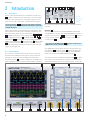
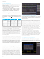
1
Mixed Signal Oscilloscope
HMO series 3000
300-500 MHz
3 0 0 - 5 0 0 MHz
xe d Si gn a l O s z i l l o s ko p
UserMiManual
HM O S e r i e 3 0 0 0
Handbuch
Benutzerhandbuch / User Manual
Deutsch
General Information Regarding the CE Marking
General Information Regarding the CE Marking
KONFORMITÄTSERKLÄRUNG
DECLARATION OF CONFORMITY
DECLARATION DE CONFORMITE
DECLARACIÓN DE CONFORMIDAD
Hersteller / Manufacturer / Fabricant / Fabricante:
HAMEG Instruments GmbH · Industriestraße 6 · D-63533 Mainhausen
Die HAMEG Instruments GmbH bescheinigt die Konformität für das Produkt
The HAMEG Instruments GmbH herewith declares conformity of the product
HAMEG Instruments GmbH déclare la conformite du produit
HAMEG Instruments GmbH certifica la conformidad para el producto
Bezeichnung: Oszilloskop
Product name: Oscilloscope
Designation:Oscilloscope
Descripción:Osciloscopio
Typ / Type / Type / Tipo:
HMO3002, HMO3004
mit / with / avec / con:
HO730
Optionen / Options /
Options / Opciónes: HO720, HO740
mit den folgenden Bestimmungen / with applicable regulations /
avec les directives suivantes / con las siguientes directivas:
EMV Richtlinien / EMC Directives / Directives CEM / Directivas IEM:
2004/108/EG;
Niederspannungsrichtlinie / Low-Voltage Equipment Directive / Directive des
equipements basse tension / Directiva de equipos de baja tensión:
2006/95/EG
Angewendete harmonisierte Normen / Harmonized standards applied /
Normes harmonisées utilisées / Normas armonizadas utilizadas:
Sicherheit / Safety / Sécurité / Seguridad:
DIN EN 61010-1; VDE 0411-1: 07/2011
Überspannungskategorie / Overvoltage category / Catégorie de surtension /
Categoría de sobretensión: II
Verschmutzungsgrad / Degree of pollution / Degré de pollution /
Nivel de polución: 2
Elektromagnetische Verträglichkeit / Electromagnetic compatibility /
Compatibilité électromagnétique / Compatibilidad electromagnética:
EMV Störaussendung / EMI Radiation / Emission CEM / emisión IEM:
DIN EN 61000-6-3: 09/2007 (IEC/CISPR22, Klasse / Class / Classe / classe B)
VDE 0839-6-3: 04/2007
Störfestigkeit / Immunity / Imunitee / inmunidad:
DIN EN 61000-6-2; VDE 0839-6-2: 03/2006
Oberschwingungsströme / Harmonic current emissions / Émissions de courant
harmonique / emisión de corrientes armónicas:
DIN EN 61000-3-2; VDE 0838-2: 06/2009
Spannungsschwankungen u. Flicker / Voltage fluctuations and flicker /
Fluctuations de tension et du flicker / fluctuaciones de tensión y flicker:
DIN EN 61000-3-3; VDE 0838-3: 03/2010
Datum / Date / Date / Fecha
08. 04. 2013
Unterschrift / Signature / Signatur / Signatura
HAMEG measuring instruments comply with regulations of the EMC Directive. HAMEG is basing the conformity assessment on prevailing generic and
product standards. In cases with potentially different thresholds, HAMEG
instruments apply more rigorous test conditions. Thresholds for business and
commercial sectors as well as small business are applicable for interference
emission (class 1B). As to the interference immunity, the standard thresholds
for the industrial sector apply.
Measurement and data lines connected to the measuring instrument
significantly affect compliance with specified thresholds. Depending on the
respective application, utilized lines may differ. In regards to interference
emission and immunity during measurements, it is critical that the following
terms and conditions are observed:
1. Data Cables
It is imperative to only use properly shielded cables when connecting measuring instruments and interfaces to external devices (printers, computers,
etc.). Unless the manual prescribes an even shorter maximum cable length,
data cables (input/output, signal/control) may not exceed a length of 3
meters and may not be used outside of buildings. If the instrument interface
includes multiple ports for interface cables, only one cable at a time may be
connected. Generally, interconnections require double-shielded connecting
cables. The double-shielded cable HZ72 (available at HAMEG) is well suitable
as IEEE BUS cable.
2. Signal Cables
In general, measuring cables for the transmission of signals between measuring point and measuring instrument should be kept as short as possible.
Unless an even shorter maximum cable length is prescribed, signal cables
(input/output, signal/control) may not exceed a length of 3 meters and may
not be used outside of buildings. All signal cables must be shielded (coaxial
cable RG58/U). It is important to ensure proper ground connection. Signal
generators require the use of double-shielded coaxial cables (RG223/U,
RG214/U).
3. Impact on Measuring Instruments
If strong high-frequency electric and magnetic fields are present, it may
occur despite diligent measurement setup that unwanted signal units are
injected into the measuring instrument via connected measuring cables. This
will not damage the HAMEG measuring instrument or put it out of operation.
In some cases, these circumstances may cause the measuring value to
slightly exceed specifications.
4. interference Immunity in Oscilloscopes
4.1 Electromagnetic RF Field
If strong high-frequency electric and magnetic fields are present, fieldrelated overlays in the measuring signal may become visible. Coupling of
these fields may occur via power supply, measuring and control cables and/
or via indirect radiation. This may affect both the measurement object and
the oscilloscope.
General
Information
Regarding
the CE
Marking
Although the oscilloscope is shielded by the metal casing, direct radiation
may occur through the monitor opening. Since the
bandwidth of each amplifier stage is higher than the total bandwidth of the
oscilloscope, overlaps with a frequency noticeably higher than the measuring bandwidth of –3dB may become visible.
4.2 Fast Transients / Discharging Static Electricity
Fast transients (Burst) and direct coupling via power supply or indirect
coupling (capacitive) via measuring and control cables may trigger the event.
Direct or indirect static discharge (ESD) may also affect the trigger. Since the
triggering and signal display should also occur for signals with low signal
amplitudes (<500µV), it is inevitable that these types of signals (> 1kV)
activate the triggering and display simultaneously.
HAMEG Instruments GmbH
2
Holger Asmussen
General Manager
Content
Content
General Information Regarding the
CE Marking. . . . . . . . . . . . . . . . . . . . . . . . . . . . . 2
Content. . . . . . . . . . . . . . . . . . . . . . . . . . . . . . . 3
1
Installation and safety
instructions. . . . . . . . . . . . . . . . . . . . . . . . . . . . 4
1.1Symbols . . . . . . . . . . . . . . . . . . . . . . . . . . . . . . . . . . . 4
1.2 Setting Up the Instrument. . . . . . . . . . . . . . . . . . . . . 4
1.3Safety . . . . . . . . . . . . . . . . . . . . . . . . . . . . . . . . . . . . . 4
1.4 Intended Operation. . . . . . . . . . . . . . . . . . . . . . . . . . . 5
1.5 Ambient Conditions . . . . . . . . . . . . . . . . . . . . . . . . . . 5
1.6 Warranty and Repair. . . . . . . . . . . . . . . . . . . . . . . . . . 5
1.7Maintenance. . . . . . . . . . . . . . . . . . . . . . . . . . . . . . . . 5
1.8 Measuring Category 0 . . . . . . . . . . . . . . . . . . . . . . . . 6
1.9 Mains Voltage. . . . . . . . . . . . . . . . . . . . . . . . . . . . . . . 6
1.10 Batteries and Rechargeable Batteries/Cells. . . . . . . . 6
1.11 Product Disposal. . . . . . . . . . . . . . . . . . . . . . . . . . . . . 7
2Introduction. . . . . . . . . . . . . . . . . . . . . . . . . . . . 8
2.1 Front View. . . . . . . . . . . . . . . . . . . . . . . . . . . . . . . . . . 8
2.2 Control Panel. . . . . . . . . . . . . . . . . . . . . . . . . . . . . . . . 8
2.3Screen. . . . . . . . . . . . . . . . . . . . . . . . . . . . . . . . . . . . . 9
2.4 Rear View. . . . . . . . . . . . . . . . . . . . . . . . . . . . . . . . . . 9
2.5Options. . . . . . . . . . . . . . . . . . . . . . . . . . . . . . . . . . . 10
2.6 General Operating Concept. . . . . . . . . . . . . . . . . . . 10
2.7 Basic Settings and Integrated Help. . . . . . . . . . . . . 11
2.8 Bus Signal Source. . . . . . . . . . . . . . . . . . . . . . . . . . . 12
2.9 Updates to Instrument Firmware and Help. . . . . . . 12
2.10 Upgrade with Software Options . . . . . . . . . . . . . . . 12
2.11 Self Alignment . . . . . . . . . . . . . . . . . . . . . . . . . . . . . 13
2.12 Logic Probe Self Alignment. . . . . . . . . . . . . . . . . . . 14
3
Quick Start Guide. . . . . . . . . . . . . . . . . . . . . . . 14
3.1 Instrument Positioning and Start-Up. . . . . . . . . . . . 14
3.2 Connecting a Probe and Capturing a Signal . . . . . . 14
3.3 Display of signal details . . . . . . . . . . . . . . . . . . . . . . 15
3.4 Cursor Measurements . . . . . . . . . . . . . . . . . . . . . . . 15
3.5 Automatic Measurements . . . . . . . . . . . . . . . . . . . . 16
3.6 Mathematical Settings. . . . . . . . . . . . . . . . . . . . . . . 17
3.7 Storing Data . . . . . . . . . . . . . . . . . . . . . . . . . . . . . . . 17
4
Vertical System . . . . . . . . . . . . . . . . . . . . . . . . 18
4.1Coupling. . . . . . . . . . . . . . . . . . . . . . . . . . . . . . . . . . 18
4.2 Sensitivity, Y Positioning and Offset . . . . . . . . . . . . 19
4.3 Bandwidth Limit and Signal Inversion. . . . . . . . . . . 19
4.4 Probe Attenuation and Unit Selection
(Volt/Ampere). . . . . . . . . . . . . . . . . . . . . . . . . . . . . . 19
4.5 Threshold Setting. . . . . . . . . . . . . . . . . . . . . . . . . . . 20
4.6 Naming a Channel . . . . . . . . . . . . . . . . . . . . . . . . . . 20
5
Horizontal System (time base). . . . . . . . . . . . . 21
5.1 Acquisition modes RUN and STOP . . . . . . . . . . . . . 21
5.2 Time Base Settings. . . . . . . . . . . . . . . . . . . . . . . . . . 21
5.3 Acquisition modes . . . . . . . . . . . . . . . . . . . . . . . . . . 21
5.4 Interlace Mode. . . . . . . . . . . . . . . . . . . . . . . . . . . . . 24
5.5 ZOOM function. . . . . . . . . . . . . . . . . . . . . . . . . . . . . 24
5.6 Navigation function . . . . . . . . . . . . . . . . . . . . . . . . . 25
5.7 Marker function . . . . . . . . . . . . . . . . . . . . . . . . . . . . 25
5.8 Search Function
. . . . . . . . . . . . . . . . . . . . . . . . . . . . 25
6
Trigger System. . . . . . . . . . . . . . . . . . . . . . . . . 26
6.1 Trigger Modes Auto, Normal and Single. . . . . . . . . 26
6.2 Trigger Sources. . . . . . . . . . . . . . . . . . . . . . . . . . . . . 26
6.3 Slope Trigger. . . . . . . . . . . . . . . . . . . . . . . . . . . . . . . 27
6.4 Puls Trigger. . . . . . . . . . . . . . . . . . . . . . . . . . . . . . . . 27
6.5 Logic Trigger. . . . . . . . . . . . . . . . . . . . . . . . . . . . . . . 28
6.6 Hold Off. . . . . . . . . . . . . . . . . . . . . . . . . . . . . . . . . . . 29
6.7 Video Trigger. . . . . . . . . . . . . . . . . . . . . . . . . . . . . . . 29
7
Signal Display. . . . . . . . . . . . . . . . . . . . . . . . . . 30
7.1 Display Settings . . . . . . . . . . . . . . . . . . . . . . . . . . . . 30
7.2 Usage of the Virtual Screen. . . . . . . . . . . . . . . . . . . 31
7.3 Signal Intensity Display and Persistence Function . 31
7.4 XY Display. . . . . . . . . . . . . . . . . . . . . . . . . . . . . . . . . 32
8Measurements. . . . . . . . . . . . . . . . . . . . . . . . . 33
8.1 Cursor Measurements . . . . . . . . . . . . . . . . . . . . . . . 33
8.2 Automatic Measurements . . . . . . . . . . . . . . . . . . . . 34
9Analysis . . . . . . . . . . . . . . . . . . . . . . . . . . . . . . 37
9.1 Mathematical Functions . . . . . . . . . . . . . . . . . . . . 37
9.1.1 Quick Mathematics. . . . . . . . . . . . . . . . . . . . . . . . . . 37
9.1.2 Formula Editor . . . . . . . . . . . . . . . . . . . . . . . . . . . . . 37
9.2 Frequency Analysis (FFT). . . . . . . . . . . . . . . . . . . . . 39
9.3 Quick View. . . . . . . . . . . . . . . . . . . . . . . . . . . . . . . . 40
9.4 PASS/FAIL Test Based on Masks. . . . . . . . . . . . . . . 40
10 Documentation, Storage and Recall . . . . . . . . 42
10.1 Instrument Settings
. . . . . . . . . . . . . . . . . . . . . . 42
10.2References . . . . . . . . . . . . . . . . . . . . . . . . . . . . . . . . 43
10.3Curves. . . . . . . . . . . . . . . . . . . . . . . . . . . . . . . . . . . . 43
10.4 Sreenshots . . . . . . . . . . . . . . . . . . . . . . . . . . . . . . 44
10.5 Formula Sets. . . . . . . . . . . . . . . . . . . . . . . . . . . . . . . 45
10.6 FILE/PRINT Key Definition . . . . . . . . . . . . . . . . . . . . 45
11Mixed-Signal-Operation. . . . . . . . . . . . . . . . . . 46
11.1 Logic Trigger for Digital Input . . . . . . . . . . . . . . . 46
11.2 Display Functions for the Logic Channels . . . . . . 46
11.3 Cursor Measurements for Logic Channels . . . . . . . 47
11.4. Automatic Measurements for Logic Channels . . . . 47
12 Serial BUS
analysis. . . . . . . . . . . . . . . . . . . . . . . . . . . . . . . 48
12.1 The options HOO10, HOO11 and HOO12. . . . . . . . . 48
12.2 Serial Bus Configuration . . . . . . . . . . . . . . . . . . . . 48
12.2.1BUS Table. . . . . . . . . . . . . . . . . . . . . . . . . . . . . . . . . 49
12.3 Parallel BUS. . . . . . . . . . . . . . . . . . . . . . . . . . . . . . . . 49
12.4I2C BUS. . . . . . . . . . . . . . . . . . . . . . . . . . . . . . . . . . . 49
12.5 SPI / SSPI BUS . . . . . . . . . . . . . . . . . . . . . . . . . . . . . 51
12.6 UART/RS-232 BUS. . . . . . . . . . . . . . . . . . . . . . . . . . 53
12.7 CAN BUS. . . . . . . . . . . . . . . . . . . . . . . . . . . . . . . . . . 55
12.8 LIN BUS . . . . . . . . . . . . . . . . . . . . . . . . . . . . . . . . . . 57
13 Remote control. . . . . . . . . . . . . . . . . . . . . . . . . 58
13.1Ethernet. . . . . . . . . . . . . . . . . . . . . . . . . . . . . . . . . . . 58
13.2USB. . . . . . . . . . . . . . . . . . . . . . . . . . . . . . . . . . . . . . 59
13.3 RS-232 (option HO720). . . . . . . . . . . . . . . . . . . . . . . 59
13.4 IEEE 488.2 / GPIB (Option HO740): . . . . . . . . . . . . . 59
14 Technical Data . . . . . . . . . . . . . . . . . . . . . . . . . 60
15Appendix . . . . . . . . . . . . . . . . . . . . . . . . . . . . . 63
15.1 List of figures . . . . . . . . . . . . . . . . . . . . . . . . . . . . . . 63
15.2Glossary . . . . . . . . . . . . . . . . . . . . . . . . . . . . . . . . . . 64
3
Installation and safety instructions
1 Installation and
safety
instructions
B
Removing the handle (Pos. F)
C
1.1Symbols
(1)
(2)
(5)
A
(3)
(6)
G
(4)
C
E
(7)
D
F
B
(8)
Symbol 1: Caution, general danger zone –
Refer to product documentation
Symbol 2: Risk of electric shock
Symbol 3: Ground
Symbol 4: Stop! – Risk harm to instrument
Symbol 5: PE terminal
Symbol 6: ON/OFF supply voltage
Symbol 7: Stand by display
Symbol 8: Ground terminal
D
A
E
1.2 Setting Up the Instrument
As shown in the illustrations, the handle can be pivoted
into different positions:
A and B = Carrying position
C, D and E = Operating positions using different angles
F = Position to remove the handle.
G = Position using equipment feet, stacking position and
to transport in the original packaging.
Removing/attaching the handle bar: The handle bar
may be removed in position F by pulling it out further. To
attach the handle bar, proceed in the reverse order.
Caution!
To change the position of the handle, the oscilloscope must be
placed in a safe position so that it will not fall down (e.g. on a
table). Then the handle knobs must be simultaneously pulled on
both sides and pivoted in the direction of the desired position. If
the handle knobs are not pulled out while pivoting them into the
desired position, they may lock into the nearest locking position.
1.3Safety
This instrument was built in compliance with VDE 0411
part 1, safety regulations for electrical measuring instruments, control units and Iaboratory equipment. It has been
tested and shipped from the plant in safe condition. It is in
compliance with the regulations of the European standard
EN 61010-1 and the international standard IEC 1010-1. To
maintain this condition and to ensure safe operation, the
4
Operating positions
Carrying positions
Stacking positions
Fig. 1.1: Various positions for HMO instruments
user must observe all instructions and warnings given in
this operating manual. Casing, chassis and all measuring ports/terminals are connected to a protective earth
conductor/safety ground of the mains. The instrument is
designed in compliance with the regulations of protection
class I.
The exposed metal parts have been tested against the
main poles with 2200 VDC voltage.
For safety reasons, the instrument may only be connected
to properly installed safety socket outlets. The power plug
must be inserted before signal circuits may be connected.
Separating the grounds is prohibited. If it is assumed that
a safe operation is no longer possible, the instrument
must be shut down and secured against any unintended
operation.
Safe operation can no longer be assumed:
❙❙ If the instrument shows visible damage,
❙❙ If the instrument includes loose parts,
❙❙ If the instrument no longer functions properly,
❙❙ After an extended period of storage under unfavorable
conditions (e.g. outdoors or in damp rooms),
Installation and safetyinstructions
❙❙ After rough handling during transport (e.g. packaging that
does not meet the minimum requirements by post office,
railway or forwarding agency).
1.4 Intended Operation
CAUTION! The measuring instrument is intended only
for use by personnel familiar with the potential risks of
measuring electrical quantities. For safety reasons, the
oscilloscope may only be connected to properly installed
safety socket outlets. Separating the grounds is prohibited.
The power plug must be inserted before signal circuits
may be connected. The oscilloscope is designed for use in
the following sectors: Industrial sector, Home, Business or
commercial sectors and Small businesses.
Use the measurement instrument only with original HAMEG
measuring equipment, measuring cables and power cord. Before
each measurement, measuring cables must be inspected for damage and replaced if necessary. Damaged or worn components
can damage the instrument or cause injury.
To disconnect from the mains, the rubber connector on the back
panel has to be unplugged.
The oscilloscope is designed for indoor use only. Before
each measurement, you need to verify at a known source
if the measurement instrument functions properly.
1.5 Ambient Conditions
Permissible operating temperatures during the operations
range from +5 °C to +40 °C. During storage or transportation the temperature may be between –20 °C and +70 °C. In
case of condensation during transportation or storage, the
Do not obstruct the ventilation holes!
instrument will require approximately two hours to dry and
reach the appropriate temperature prior to operation. The
oscilloscope is designed for use in a clean and dry indoor
environment. Do not operate with high dust and humidity
levels, if danger of explosion exists or with aggressive
chemical agents. Any operating position may be used;
however, adequate air circulation must be maintained.
For continuous operation, a horizontal or inclined position
(integrated stand) is preferable. The maximum operating
altitude for the instrument is 2000 m above sea level.
Specifications with tolerance data apply after a warm up
period of at least 30 minutes at a temperature of 23 °C
(tolerance ±2°C). Specifications without tolerance data are
average values.
1.6 Warranty and Repair
HAMEG instruments are subject to strict quality controls.
Prior to leaving the manufacturing site, each instrument
undergoes a 10-hour burn-in test. This is followed by extensive functional quality testing to examine all operating
modes and to guarantee compliance with the specified
technical data. The testing is performed with testing equipment that is calibrated to national standards. The statutory
warranty provisions shall be governed by the laws of the
country in which the HAMEG product was purchased. In
case of any complaints, please contact your supplier.
Applicable only in EU countries:
To accelerate claims, customers in EU countries may also
contact HAMEG directly for repairs. The HAMEG customer
service is available for repair services even once the warranty period ends.
Return Material Authorization (RMA):
In any event, before returning an instrument, request
a RMA number either via Internet (http://www.hameg.
com) or by fax. If you need technical support or a suitable
original packaging, please contact the HAMEG service
department:
HAMEG Instruments GmbH
Service
Industriestr. 6
D-63533 Mainhausen
Telefon: +49 (0) 6182 800 500
Telefax: +49 (0) 6182 800 501
E-Mail: [email protected]
Any adjustments, replacements of parts, maintenance
or repair may be carried out only by authorized HAMEG
technical personnel. Only original parts may be used for
replacing parts relevant to safety (e.g. power switches,
power transformers, fuses). A safety test must always
be performed after parts relevant to safety have been
replaced (visual inspection, PE conductor test, insulation
resistance measurement, leakage current measurement,
functional test). This helps to ensure the continued safety
of the product.
The product may only be opened by authorized and
qualified personnel. Before any work is performed on
the product or before the product is opened, it must be
disconnected from the AC supply network. Otherwise,
personnel will be exposed to the risk of an electric
shock.
1.7Maintenance
❙❙ Clean the outer case of the oscilloscope at
regular intervals, using a soft, lint-free dust cloth.
❙❙ Before cleaning the instrument, please make sure that it
has been switched off and disconnected from all power
supplies.
❙❙ No instrument parts may be cleaned with alcohol or other
cleaning agents!
The display may only be cleaned with water appropriate
glass cleaner (not with alcohol or other cleaning agents).
Follow this step by rubbing the display down with a dry,
5
Installation and safetyinstructions
clean and lint-free cloth. Do not allow cleaning fluid to enter the instrument. The use of other cleaning agents may
damage the labeling or plastic and laquered surfaces.
1.8 Measuring Category 0
This oscilloscope is designed for measurements on circuits
that are only indirectly connected to the mains or not connected at all. The instrument is in compliance with measuring category 0. Make sure the entry voltage does not
exceed 200 V (peak value),150 VRMS at 1 MΩ input impedance and 5 VRMS at 50 Ω input impedance.
a single unit. You need to first disconnect the power cord
from the connector before you can safely replace the fuse
(as long as the fuse holder is undamaged). Next the fuse
holder must be pried out using a screwdriver. The starting point is a slot next to the contacts. Then the fuse can
be forced out of its mounting and must be replaced by an
identical fuse (please find information about the fuse type
below). The fuse holder will be inserted against the spring
pressure until it locks into place. The use of mended fuses
or to short circuit the fuse holder is prohibited. Resulting
damages are not covered by the warranty.
Fuse type: IEC 60127 - T2.5H 250V, size 5 x 20 mm
The maximum value allowed for transient overvoltages is
200 V (peak value). When performing measurements in
circuits with transient overvoltages higher than category
0, make sure that no transient overvoltages higher than
category 0 occur at the measurement input. To ensure
compliance, it is necessary to only use probes that have
been manufactured and tested in accordance with DIN EN
61010-031. When performing measurements in category
II, III or IV circuits, it is mandatory to insert a probe that reduces the voltage so that no transient overvoltages higher
than category 0 will be applied to the instrument. Direct
measurements (without galvanic isolation) to category
II, III or IV circuits are prohibited! The measuring circuits
are considered not connected to the mains if an isolation
transformer in compliance with safety class II is used. It is
also possible to perform measurements on the mains if appropriate transformers (e.g. current connectors) are used
that are in compliance with safety class II. The measurement category (for which the manufacturer specified the
required transformer) must be observed.
Measurement Categories
The measurement categories refer to transients from the
power system. Transients are short, very fast (steep) current and voltage variations which may occur periodically
and non-periodically. The level of potential transients
increases as the distance to the source of the low voltage
installation decreases.
Measurement CAT IV: Measurements at the source of
the low voltage installations (e.g. meters)
Measurement CAT III: Measurements in building installations (e.g. power distribution installations, power switches,
firmly installed sockets, firmly installed engines etc.).
Measurement CAT II: Measurements on circuits electronically directly connected to the mains (e.g. household
appliances, power tools, etc.)
Measurement category 0 (previously Measurement
CAT I): Electronic devices and fused circuits in devices.
1.9 Mains Voltage
The instrument applies 50 and 60 Hz mains voltages ranging from 100 V to 240 V (tolerance ±10%). Mains voltage
switching is therefore not required. The input line fuse is
accessible externally. Power socket and fuse holder form
6
1.10 Batteries and Rechargeable Batteries/Cells
If the information regarding batteries and rechargeable batteries/cells is not observed either at all or to the extent necessary, product users may be exposed to the risk of explosions,
fire and/or serious personal injury, and, in some cases, death.
Batteries and rechargeable batteries with alkaline electrolytes
(e.g. lithium cells) must be handled in accordance with the EN
62133 standard.
1. Cells must not be disassembled, opened or crushed.
2. Cells and batteries may not be explosed to heat or fire.
Storage in direct sunlight must be avoided. Keep cells
and batteries clean and dry. Clean soiled connectors
using a dry, clean clothes.
3. Cells or batteries must not be short-circuited. Cells or
batteries must not be stored in a box or in a drawer
where they can short-circuit each other, or where they
can be short-circuited by other conductive materials.
Cells and batteries must not be removed from their original packaging until they are ready to be used.
4. Keep cells and batteries out of reach of children. Seek
medical assistance immediately if a cell or battery was
swallowed.
5. Cells and batteries must not be exposed to any mechanical shocks that are stronger than permitted.
6. If a cell develops a leak, the fluid must not be allowed
to come into contact with the skin or eyes. If contact
occurs, wash the affected area with plenty of water
and seek medical assistance.
7. Improperly replacing or charging cells or batteries that
contain alkaline electrolytes (e.g. lithium cells) can
cause explosions. Replace cells or batteries only with
the matching type in order to ensure the safety of the
product.
8. Cells and batteries must be recycled and kept separate
from residual waste. Cells and batteries must be recycled and kept separate from residual waste. Recharge-
Installation and safetyinstructions
able batteries and normal batteries that contain lead,
mercury or cadmium are hazardous waste. Observe
the national regulations regarding waste disposal and
recycling.
1.11 Product Disposal
Fig. 1.2:
Product labeling in accordance with EN 50419
The German Electrical and Electronic Equipment Act implements the following EC directives:
❙❙ 2002/96/EC (WEEE) for electrical and electronic
equipment waste and
❙❙ 2002/95/EC to restrict the use of certain hazardous
substances in electronic equipment (RoHS directive).
Once its lifetime has ended, this product should be disposed of separately from your household waste. The disposal at municipal collection sites for electronic equipment
is also not permitted. As mandated for all manufacturers
by the German Electrical and Electronic Equipment Act
(ElektroG), HAMEG assumes full responsibility for the ecological disposal or the recycling at the end-of-life of their
products.
Please contact your local service partner to dispose of the
product.
7
Introduction
2 Introduction
3
4
8
5
17
the control
panel
If you press the AUTOSET button 15 longer then 3 seconds, the
HMO will be reset to its default settings!
The ANALYZE section allows users to directly access the
FFT displays 9 , the Quick View 10 display (all important
parameters of the actual signal display), the PASS/FAIL
mask test, and the AUTOMEASURE settings 11 .
The General section includes the Save/Recall 12 key. With
this option, you can control the settings to load and save
instrument settings, reference signals, signals, screen dis1
55
8
14
Section A
This section includes the CURSOR/MENU, ANALYZE
and GENERAL sections. The CURSOR/MENU section includes cursor functions 6 8 , universal knob 4 , Intens/
Persist control switch 7 and the option to select the
virtual screen 5 .
2.2 Control Panel
The controls in the front panel allow access to all basic
functions while advanced settings are easily accessible
through the menu structure and gray soft menu keys.
The power button 1 is clearly set apart by its design. The
most significant controls feature colored LEDs, indicating
51 50
11
the current setting. The control panel is divided into four
sections.
main power switch on the backside, the red light will also
switch off (this will take some seconds). Furthermore you
find on the front panel the the control panel 2 , A , B , C ,
D , the BNC connectors of the analog inputs 45 to 48 , the
probe adjustment output 51 , the BUS signal source 50 , the
connectors 52 53 for the optional logic probes HO3508, a
USB port for USB sticks 54 , the TFT screen 55 and the LED
49 for showing activity on the remote interface. The two
channel instruments includes an AUX socket for external
trigger on the right side.
Fig. 2.1: Frontview of the HMO3004
15 16
Section A of
for the logic probes of type HO3508. Connecting other types may
demolish the inputs.
52
13
Fig. 2.2:
Use the connectors 52 53 for the active logic probes exclusively
53
10 12
A
2.1 Front View
On the instrument frontside you can find the power key
1 , in order to switch on the instrument or to enter standby mode. If the instrument is in stand-by mode, this key
lights up red. If the instrument is switched off using the
54
7 9
6
49
48
A
2
47
B
46 C
45 D
spiel der Sprache), die generellen
B
Einstellfunktionen der Anzeige
22
14 , das Autosetup 15 , sowie die
18
plays and Hilfe
sets of
Additional
keys enable the user
16 formulas.
integrierte
und die Taste
17 , welche
FILE/PRINT
je nach
23
13 such as language, DISPLAY
to access general
settings
Programmierung
das
direkte
19
14 , AUTO-SET 15 as well as integrated
HELP 16 and FILE/
Abspeichern von GeräteeinstelPRINT 17 . Depending on how it is programmed, FILE/ 24
lungen, Kurven, Bildschirmfotos
PRINT
enables
you to
oder
den
Ausdruck
aufdirectly
einemsave instrument settings,
25
signals and screen
displays or print on a postscript printer.
Postscriptdrucker
ermöglicht.
Introduction
2.3Screen
The HMO series is equipped with a 6.5” (16.51 cm) TFT
color monitor with LED backlight and VGA resolution
(640x480 pixels). In the default setting (no menus shown),
the screen includes 12 scale divisions on the time axis.
20
26
Abschnitt
Section BB ::
Im Bereich VERTICAL befinden
The VERTICAL section features all controls for analog
sich alle Einstellmöglichkeiten 21
27
channels,
such as
the position
für
die analogen
Kanäle,
wie die control knob 18 , the XZ
mode select
, the vertical gain
knob 20 ,
18 ,key
Y-Position
die 19Umschaltung
Abb. adjustment
2.3:
19
in
den
XY-Anzeigebetrieb
Bedienfeldabschnitt
B
,
die
the advanced menu options key 21 , the channel select
20
vertikale
Verstärkung
,
weiterkeys 22 to 25 and the optional
gehende Menüs 21 , die Kanalwahl
C
logic probes HO3508 24 25 .
22 bis 25 , sowie der optionalen
You
can
also
access
the
Logiktastköpfe HO3508 24 25 .
28
B
MATH key finden
and theSie
reference
Außerdem
hier den
22
26
Zugang
zur
Mathematik
,
den
signal settings key here 27 .
Referenzkurven-unddenBusein18
29
33
stellungen 27 .
23
Section C :
The TRIGGER
C : section includes
Abschnitt
all
options
to set
the trigger
Der Abschnitt
TRIGGER
stellt
alle
Funktionen
zum
Einstellen
28
level , to switch between
28 ,mode
des
Triggerpegels
der UmAUTO
and NORMAL
schaltung zwischen AUTO- und
29 , to set the trigger type
NORMAL-Betrieb 29 , des Trig31 , the source
, the single
31 , der32Quelle
32 , der
gertyps
sweep,
to
switch
the trigger 33 ,
einmaligen Triggerauslösung
derUmschaltungderTriggerflanslope and to set the trigger
35 , filters.
ke
sowie Additionally,
der Einstellungen
signal
you
zur Triggerfilterbedingung 36
can find status indicators, and
zur Verfügung. Zusätzlich finyou Sie
canStatusanzeigen,
see if a signal fulfills
den
ob ein
the
trigger
conditions 30 and
Signal die Triggerbedingungen
erfüllt
undwelchederFlanken
which30slope
is used 34 .
genutzt werden 34 .
19
20
30
34
24
31
35
25
32
36
26
Abb. 2.4:
21Bedienfeldabschnitt C 27
D
37
38
37
41
C
42
39
28
Section D :
Abschnitt D :
In the
HORIZONTAL
section,
Im
Abschnitt
HORIZONTAL
erfolgt
4333
29
users
can
shift
the
trigger
podie Einstellung der Horizontalposition
des Triggerzeitpunktes
sition
horizontally or setoder
anddas
40
34
30
Setzen
und
Navigieren
von
Markern
navigate markers manually,
44
37
38
39
über Drucktasten
in Schriteither step-by-step with the
31
35
ten, oder variabel mit dem kleineren
37
38
39
keys
or
alternatively
Abb. 2.5:
Drehknopf 41 . Zusätzlich lässt sich
Bedienfeldabschnitt D 36
32
by Menü
usingeine
the smaller
one ofnach
im
Suchfunktion
Ereignissen
Auswahl
41 . In theDie
the knobs einstellen.
menu,
des
oderset
STOP
Modus
erfolgt mit einer hinterleuchteten
youRUNcan also
search
criteTaste 39 , wobei im STOP Modus die Taste rot leuchtet. Die
ria for events. The illuminated
Zoom-Aktivierung 40 , die Auswahl der Erfassungsmodi 44 , die
key 39 allows the selection
43 , sowie der Zugriff auf das Zeitbasismenü
Zeitbasiseinstellung
D
oferfolgenebenfallsindiesemAbschnitt.Zusätzlichbefinden
the RUN and STOP mode.
42
37
sich
links
demmode
Bedienpanel
die Softmenütasten 2 , mit
When
theauf
STOP
is
38
41
denen
die Menüsteuerung
erfolgt.
selected,
the key will light
up
37
in red. 40 activates the zoom
42
44 selects the acquisioption,Bildschirm
2.3
39
tion modes, 43 adjusts the
Die
istand
mit 42einem
timeHMO
baseSerie
speed
en- 6,5 Zoll (16,51 cm), mit LED
hinterleuchtetemTF
ables access to the TFarbbildschirmmiteinerVGAAuflötime base
43
sung (640x480 Pixel) ausgestattet. In der Normaleinstellung
menus.
(ohne eingeblendete Menüs) verfügt der Bildschirm über 12
40
Skalenteile auf der Zeitachse. Diese wird bei Einblendung
To the left of the control
panel, you also find the soft
menu keys 2 to control the
menu options.
44
Fig. 2.3: Section B, C and D of
the control panel
Abb. 2.6: Bildschirmansicht
von Menüs auf 10 Skalenteile reduziert. Am linken Rand der
Anzeige werden Informationen zum Bezugspotential der
Kanäle mit kleinen Pfeilen markiert [1]. Die Zeile oberhalb
des Gitters enthält Status und Einstellungsinformationen,
wie die eingestellte Zeitbasis, die Triggerverzögerung und
sonstige Triggerbedingungen, die aktuelle Abtastrate und
die Erfassungsart [2]. Rechts neben dem Gitter wird ein
Fig.
2.4: Sreenfür
view
Kurzmenü
die wichtigsten Einstellungen des jeweils aktiven
Kanales
dargestellt,
welche
mit dento
Softmenütasten
If menus are shown,
this will
be reduced
10 divisions.
ausgewählt werden können [3]. Im unteren Bildschirmteil
Small arrows [1] on the left of the display indicate the
werden die Messergebnisse der automatischen Messungen und
reference
potentials
of the Einstellungen
channels. The
line
above the
Cursors, sowie
die vertikalen
der
eingeschalteten
graticule
includes
status
and
settings
information
Kanäle, Referenzen und Mathematikkurven angezeigtsuch
[4]. Im
Gitter
selbst
Signale
der eingeschalteten
Kanäle
as
time
base,werden
triggerdie
delay
and other
trigger conditions,
dargestellt.
stellt
8 Skalenteile
gleichzeitigmode
dar, verfügt
the
current Dieses
sampling
rate
and the acquisition
[2].
aber über eine virtuelle Erweiterung auf 20 Skalenteile, welche
The short menu to the right of the graticule contains the
mit Hilfe der Taste SCROLL/BAR 5 angezeigt werden können.
most important settings of the currently active channel.
You may select these settings using the soft menu keys
2.4 Measurement
Rückansichtresults for automated measurements
[3].
and cursors, settings for the activated vertical channels,
AufderRückseitedesGerätesbefindetsichdieBuchsezum
reference signals and mathematically derived curves are
Anschluss der Stromversorgung [1], der Modulschacht für die
shown
in the lower section
of the screen
[4]. Within the
Schnittstellenmodule
(USB/Ethernet,
USB/RS-232,IEEE-488)
graticule,
signals
of
the
selected
channels
are
displayed.
[2],diestandardmäßigeDVI-DBuchse[3] zum
Anschluss
externer
digitaler
Monitore
und Projektoren,
By
default,
8 scale
divisions
are shown. der
ThisBNC
canAnschluss
be extenfür den
AUX-OUT[4],
sowie derwhich
BNC Anschluss
für den externen
ded
virtually
to 20 divisions
can be displayed
using
Trigger [5].Beim2-Kanal-GerätfehltderBNCAnschlussfür
the Scroll/Bar 5 key.
den externen Trigger [5],dieserbefindetsichinder2-KanalVersion (AUX) auf der Vorderseite.
2.4 Rear View
[1]
[5] [4]
[2]
[2]
[3]
Abb.2.5:
2.7:Rear
Rückseite
HMO3004series
Serie
Fig.
panel HMO3004
The rear panel of the HMO series features the connector
11
Änderungen vorbehalten
for the power supply [1], the receptacle
for the interface
modules [2] (Ethernet/USB, USB/RS-232, IEEE-488), the
9
Introduction
standard DVI-D connector [3] to connect external digital
monitors and projectors, the BNC connector for the AUXOUT [4] and for the external trigger [5]. The 2-channel
instrument does not include the BNC connector for the
external trigger [5]. For this model, it is located on the front
panel.
2.4.1 DVI Connector
The rear panel of the oscilloscope includes a standard DVID connector to connect external monitors and projectors.
The DVI-D connector can only send digital signals. This
means it is impossible to connect monitors or beamers
via their analog inputs. The HMO series yields a DVI
signal with VGA resolution (640x480). This design enables
connectivity with all standard TFT monitors. Modern flat
screens extrapolate the signal, allowing users to see a full
screen.
Beamers can also be connected to the HMO. Ideal beamers in this case are those designed to be connected to
computers/ notebooks as these are also able to process a
640 x 480 pixel resolution.
2.5Options
The HMO series offers several options which allow the
user to expand the range of application considerably. The
following interface modules are available and may be installed by the customer in the rear receptacle (by default
equipped with a Ethernet/USB HO730 dual interface):
❙❙ HO740 (IEEE-488, GPIB, galvanically isolated)
❙❙ HO720 (combination of RS-232 and USB)
All HMO series instruments are prepared for mixed-signal
operation and include the appropriate connectors on the
front panel. Each of these connectors can be connected
to an 8-channel logic probe HO3508, allowing a maximum
of 16 digital logic channels. Other available options are the
passive 500 MHz Slimline 10:1 probe of type HZ355 (included in delivery with HMO3052 und HMO3054), passive
1000 : 1 probes with up to 4000 V of type HZO20, active
10 : 1 probes with <1pF input capacity of type HZO30, active difference amplifier probes HZ100, HZ109 and HZ115
with up to 1000 VRMS and 40 MHz, active high speed differential probes HZO40 and HZO41 with 200 or 800 MHz
bandwidth, the current probes HZO50 and HZO51 with
up to 100 kHz bandwidth and up to 1000 A, the 19” rack
mount set HZ46 and the HZ99 bag for transportation and
protection of the instruments. The options HOO10/11/12
allow the analysis of serial buses. For more information,
please refer to chapter 2.10. Additionally, you are able to
upgrade the bandwidth of the instrument by an optional
license key at any time (HOO352, HOO354, HOO452,
HOO454).
2.6 General Operating Concept
Our oscilloscopes are renowned for their ease of use. The
user-friendly operation is based on a few key principals,
recurring with various settings and functions.
10
❙❙ Keys that do not open a soft menu (e.g. SCROLL BAR)
activate a specific function; pressing this key a second
time will deactivate this function.
❙❙ Keys that call a specific function (e.g. FFT) which in turn
enable or require additional settings, activate a function
when pressed once; pressing this key a second time will
activate the soft menu for the settings while pressing it a
third time deactivates the function.
❙❙ Keys that open a soft menu when pressed once will close
the soft menu when pressed a second time.
❙❙ Depending on the requirements, the universal knob is
designed to either select a numeric value or to navigate
through submenus.
❙❙ The MENU OFF key below the soft menu keys closes the
current menu or switches to the next higher level.
❙❙ Pressing the appropriate key will activate a deactivated
channel. If a channel was already activated, selecting
another channel will change operation to the channel
whose key was pressed (its LED lights up). Pressing an
illuminated channel key for a channel that is already
displayed and selected will deactivate this channel and,
depending on availability, activate the next channel in the
sequence CH1 >CH2 >CH3 >CH4.
❙❙ If cursor measurements are activated, the COARSE/FINE
key will select the cursor with the activated universal knob
in the CURSOR/MENU section. This key is used to select
or confirm input in all menus for alphanumerical input and
for the file manager.
The soft menus include some frequently used navigation
elements as described below.
Fig. 2.6 illustrates the choice between two selection elements. To select from the three upper elements, press the
corresponding soft menu key with the element marked
in blue. A second option is shown in the two lower menu
entries. By pressing the corresponding key, you may toggle
between the options. The active selection is also marked in
blue.
Fig. 2.7 illustrates how to use these menus for functions
that have to be activated or require to have values set. You
Fig. 2.6: Selection of basic soft
Fig. 2.7: Basic soft menu elements
menu elements
for settings and navigation
Introduction
may toggle between OFF and the set value. The round
arrow on the bottom right of the menu window indicates
that the value is to be set by means of the universal knob
in the CURSOR/MENU section. A small triangle on the bottom right of a menu item indicates a lower menu level. You
can navigate additional pages on the same level by using
the last menu item. It includes the number of menu pages
on this level as well as the current page number. You can
advance to the next page by pressing the appropriate soft
menu key. Once the last page was listed, the display will
loop back to the the first page.
2.7 Basic Settings and Integrated Help
You can access important basic settings such as language
for user interface and help, general settings and interface
settings in the menu that opens when you press the
SETUP key in the GENERAL section of the control panel.
On the first page of the menu for the basic settings you
can select the language for user interface and help.
Pressing the soft menu key MISC opens a menu to select
the following settings:
❙❙ MENU OFF (selection of manual or automatic with time
limit of 4-30 seconds to hide soft menus)
❙❙ TIME REFERENCE (position to reference the trigger time
from -5 scale divisions to +5 scale divisions where 0 is the
middle and default)
❙❙ DATE & TIME (menu to set date and time)
❙❙ SOUND (menu to set any combination of sound - as beep
during setup, in the event of an error and for triggers)
❙❙ DEVICE NAME (menu to set a name with a maximum of
19 characters included with printouts)
❙❙ LOGO IN SCREENSHOT (select whether to include
HAMEG logo in the upper right of the printout or not)
❙❙ AUTOSET KEY (activate or block functionality of the
AUTOSET key)
Depending on the installed interface (USB and RS-232 by
default), the menu item INTERFACE activates the menus to
perform the interface configuration.
The menu item PRINTER includes settings for POSTSCRIPT and PCL compatible printers. When pushing this
soft menu key, a submenu opens allowing the user to select the paper format and color mode. Using the assigned
soft menu key, the top menu item PAPER FORMAT allows
you to choose from A4, A5, B5, B6, Executive, Letter and
Legal in either portrait or landscape format. Use the universal knob in the CURSOR/MENU section to select the
appropriate format.
Following the same setup procedure, the menu item
COLOR MODE allows you to choose between Grayscale,
Color and Inverted. The Grayscale mode converts the color
image to a grayscale image which can be printed on a
black-and-white postscript printer. The Color mode prints
the image in color as shown on the screen (black background). The INVERTED mode prints the color image with
a white background on a color printer thus saving toner
and ink.
When using the INVERTED mode, you should set the intensity of
the signals to about 70% to allow a high contrast print.
The menu item DEVICE INFORMATION opens a window
with detailed information on hardware and software of the
measuring instrument.
Fig: 2.9: Updating menu and information window
The second page includes the menu for the instruments
and help update (for more information, please refer to
the following chapter) and the PROBE COMP and BUS
SIGNAL SOURCE. Pushing this soft menu key will open
a submenu for the PROBE ADJUST output and the BUS
signal source. For a detailed description of the settings,
please read chapter 2.8.
The integrated help can be activated by pushing the HELP
key in the GENERAL section of the control panel. This
opens a window with explanatory text, and the HELP key
is illuminated. The text in the help window is dynamically
updated with descriptions of the corresponding setting or
function. If you no longer require help, push the HELP key
to close the HELP option. This will turn the LED indicator
for the key off and the text window for the help will close.
Fig. 2.8: Menu for basic settings
11
Introduction
2.8 Bus Signal Source
To the left of channel 1, the HMO series features four contacts generating the following signals (depending on the
respective settings):
❙❙ Square wave signal for probe compensation (default
setting), frequency 1 kHz or 1 MHz
❙❙ SPI signal, data rates 100 kBit/s, 250 kBit/s or 1 MBit/s
❙❙ I2C signal, data rates 100 kBit/s, 400 kBit/s or 1 MBit/s
❙❙ UART signal, data rates 9600 Bit/s, 115,2 kBit/s and
1 MBit/s
❙❙ Parallel stochastic bit pattern, frequency 1 kHz or 1 MHz
❙❙ Parallel counter signal, frequency 1 kHz or 1 MHz
The contact at the upper left is always ground and the
signal levels are about 1 V. The table below shows how the
four outputs S1, S2, S3 and
are used, depending on the
signal.
Signal
S1
SQUARE WAVE no signal
S2
S3
no signal
no signal
Square wave
SPI
Chip Select clock,
Low aktiv rising edge
data,
high active
no signal
I2C
no signal
Clock SCL
data SDA
no signal
UART
no signal
no signal
data
no signal
Pattern
Bit 0
Bit 1
Bit 2
Bit 3
Counter
Bit 0
Bit 1
Bit 2
Bit 3
To access the setup menu for the BUS signal source, press
the SETUP key in the GENERAL section of the control
panel, select page 2|2 and press the soft menu key PROBE
COMP. Now you may select the desired operating mode
for the BUS signal source. For each mode of operation,
an image with the corresponding pattern of signals on the
contacts is displayed. By pressing a soft menu key, you
can open a submenu with the speed setting of the selected operating mode.
The following options are available for the SQUARE WAVE
signal for probe compensation: 1 kHz for the low frequency
compensation, 1 MHz for the high frequency compensation
or AUTOMATIC (default setting). In the Automatic mode,
the output will provide 1 kHz at time bases from 100 µs
and provide 1 MHz at smaller time bases. These different
signals allow users to become familiar with and verify the
settings for the parallel and optional serial BUS analysis.
2.9 Updates to Instrument Firmware and Help
The HMO series is constantly being advanced. You can
download the current firmware at www.hameg.com.
Firmware and help are packed in one ZIP file. Depending
on the required extent of the update, the ZIP file might include either all updates or simply the instrument firmware,
for instance. After downloading the ZIP file, unpack the
data to the base directory of a USB stick. Then connect
the USB stick with the USB port of the oscilloscope and
press the SETUP key in the GENERAL section of the control panel. The menu item UPDATE can be found on page
2|2. Selecting this menu item opens a window displaying
12
Fig. 2.10: Menu and information window for help updates
version number, date and build information of the currently
installed firmware. Instrument firmware or help can be updated at this point.
Pressing the soft menu key to update the instrument firmware will result in a search for the corresponding file on
the USB stick. The information for the new firmware to be
installed will then be displayed on the stick below the row
labeled NEW:. The version number will be displayed in red
in case the existing firmware on the instrument is identical
to the latest version; otherwise the version number will
be shown in green. Only if this is the case, press the soft
menu EXECUTE to start the update. Choose the HELP
menu item in the Update menu if you intend to update the
help or add a new language for help.
The information window will now display all installed
languages, the date and relevant information about the
languages available on the stick. The soft menu allows you
to add, remove or update languages. Please note the date
format (YYYY-MM-DD) in compliance with multilingual
help ISO 8601 standards.
2.10 Upgrade with Software Options
The HMO series may be upgraded with options made
available by entering a licence key. At this time, options
HOO10/HOO11/HOO12 and und HOO352/HOO354/
HOO452/HOO454 are available. The option HOO10 allows
Fig. 2.11: „UPGRADE“ menu.
Introduction
triggering and decoding of up to two serial buses I2C, SPI,
UART/RS-232 on digital channels (with option HO3508)
and on analog channels. HOO11 allows these features only
on analog channels and with only one BUS. HOO12 allows
triggering and decoding of up to two serial buses CAN
and LIN both on analog and digital channels. The options
HOO352, HOO354, HOO452 and HOO454 allows you to
upgrade the bandwidth via license key.
accuracy, offset, time base and several trigger settings and
saves the identified correction data internally.
The instrument must have reached the required operating temperature (switched on for at least 20 minutes) and all inputs must
be unused, in other words all cables and probes must be removed
from the inputs.
To start the self alignment in the SETUP menu, go to page
2|2, press the soft menu key SELF ALIGNMENT and press
the START key. The procedure will run for about 5-10 minutes. Each step and its corresponding progress will be shown
in a bar display. After completion of a successful self alignment, you will see a similar message as shown in Fig 2.13.
Fig. 2.12: Manual licence key input.
Typically, you will receive the licence key by email as a file
attachment (name: SERIAL NUMBER.hlk). The attached
ASCII file may be opened with an editor. This allows you to
read the actual key in plain text. You can choose between
two methods to enable the desired option with this key: an
automated reading or manual input.
The automated reading via USB stick is the fastest and
easiest method. Store the licence file on a USB stick and
then install it to the instrument using the FRONT USB
port. Press the SETUP key in the GENERAL section of the
HMO control panel to open the SETUP menu. You will
find the LICENCES menu on page 2|2. The following menu
appears:
Press the soft menu key READ KEYS from licence file to
open the file manager. Select the required licence file with
the universal knob in the CURSOR/MENU section and then
use the soft menu key LOAD to load it. This will load the
licence key, making the option instantly available by restarting the instrument.
Fig. 2.13: Successful self alignment
Press the soft menu key EXIT to close the Self Alignment
menu. Abort the self alignment by pressing the soft menu
key ABORT. Aborting the self alignment procedure should
be the exception, e.g. if you failed to remove all probes
from the inputs. Once the procedure has been aborted, it
is important to carry out a complete self alignment.
If an error occurs during the self alignment although it has been
carried out as described, please send the exported .log file (see
Self Alignment menu) to [email protected]. You can save the
.log file to a USB stick.
Alternatively, you can enter the licence key manually.
Select the menu UPGRADE and press the soft menu key
INPUT KEY manually. This will open an input window. Use
the universal knob in the CURSOR/MENU section and the
ENTER key to enter the licence key manually. After entering the complete key, press the soft menu key ACCEPT to
confirm the entry. The option will be activated after restarting the instrument.
2.11 Self Alignment
The HMO series features an integrated self alignment
procedure to achieve the highest possible accuracy. During the standard self alignment the HMO adjusts vertical
Fig. 2.14: Logic probe self alignment (refer to page 14)
13
Introduction
2.12 Logic Probe Self Alignment
The self alignment for the logic probe primarily aligns the
switching levels.
3 Quick Start Guide
To start the self alignment for the logic probe, it is necessary that the logic probe type HO3508 is connected to
the HMO. It is imperative that the bit connectors are not
connected. To start the process, select the menu item
LOGIC PROBE SELF ALIGNMENT. The process is similar
to the basic instrument alignment but it only takes a few
seconds. (please refer to Fig. 2.14 on page 13).
The following chapter is an introduction to the most important HMO oscilloscope features and settings allowing
you to use the instrument promptly. The integrated calibrator signal output is used as the signal source which
means that the first steps will not require any additional
instruments.
3.1 Instrument Positioning and Start-Up
To optimally set up the instrument, position the handle so
that the display will be inclined slightly upwards (please
see chapter 1.1 on how to position the handle). Plug the
power cord into the rear panel connector. To start the instrument, press the red On/Off key 1 on the front panel.
The display appears after a few seconds, and the oscilloscope is ready for operation. Press the AUTOSET key 15
for at least 3 seconds. This will reset the most important
oscilloscope settings to their default settings.
3
4
7 9
6
10 12
13
15 16
A
Fig. 3.1:
Section A of
5
8
11
14
17
the control
panel
3.2 Connecting a Probe and Capturing a Signal
Make sure to align the passive probes prior to their first use. For
more information, please refer to the probe manual. Place the
probe in the appropriate position on the ADJ. output. The tip
will be accepted by the hole of the right output and the ground
connection connects with the left output, as shown in Fig. 4.3 in
chapter 4.
Take one of the provided probes HZ350 resp. HZ355 and
remove the protective cap from the tip. Apply the probe
Fig. 3.2: Screen display after connection of the probe
14
Quick Start Guide
the knob CCW until you can read “TB:5ms” in the upper
left corner of the screen. Press the ZOOM key 40 .
You will see the following two window display: The
upper section of the window displays the entire captured
signal whereas the lower section shows an enlarged section. Use the time base knob to select the zoom factor. The
small knob allows you to determine the horizontal position
of the section.
Fig. 3.3: Screen display after changing to DC coupling
compensation box to the BNC connector for channel 1 and
turn the black knob to the right until it latches into place.
Fig. 3.6: Zoom function
Press the ZOOM key 40 again to deactivate the zoom
mode.
Fig. 3.4: Screen display after Autosetup
On the right hand side of the screen, you will see the short
menu for channel 1. Press the soft menu key to the right of
each menu item to select frequently used settings. Press
the top soft menu key to change the input coupling to DC.
IMPORTANT: Active settings are marked in blue.
Briefly press the AUTOSET key once 15 . After a few seconds, the oscilloscope will have automatically selected the
sensitivity, time base and trigger settings. A square wave
D
signal will now be shown.
37
38
37
3.3 Display of signal
details
With the time base knob 43
you can change the displayed
time window. Turning it CCW
increases the time base. The
memory depth of 4 MB per
channel allows you to capture
wide time windows with high
resolution. Continue to turn
3.4 Cursor Measurements
After displaying and reviewing the signal, the next step
will introduce cursor measurements of the signal. Again,
briefly press the AUTOSET key once followed by the CURSOR/MEASURE key. You can now select the desired type
of measurement cursor from the menu. Press the top
soft menu key MEASURE TYPE to open the appropriate
selection menu. You can specify your selection with the
universal knob in the CURSOR/MENU section of the control panel. Turn the knob CCW until the entry “V marker“
is marked in blue. Press the MENU OFF key to close the
menu or wait until it automatically closes after a few seconds. Now two cursors will be shown along the signal
as well as the measurement results on the bottom of the
41
42
39
43
40
44
Fig. 3.5: Section D of the
control panel with zoom key
Fig. 3.7: Cursor measurements
15
Quick Start Guide
display. Press the universal knob to select the active cursor
and turn the universal knob to position the cursor.
this mode, press the CH2 key 23 to activate CH2 and press
the AUTO MEASURE 11 key to open the menu as displayed below.
The cursor measurement results will be shown on the
bottom of the display. In this example with the entry “V
marker”, the display includes the voltage at both cursor
positions, their difference, and the time difference between the cursor positions. To switch off the cursor, press
the CURSOR MEASURE key again.
3.5 Automatic Measurements
In addition to cursor measurements, automatic measurements can display the most important signal parameters.
Your HMO offers two options:
❙❙ Display definition of 6 parameters from varying sources,
❙❙ Quick display of all important parameters of one source
by use of the QUICK VIEW feature.
Please change the time base to 100 µs per scale division
and press the QUICKVIEW 10 key. You will see the following display:
Fig. 3.9: AutoMeasure menu
Pressing the MEAS. PLACE soft key will display a list.
Use the universal knob in the CURSOR/MENU section to
choose the appropriate measurement place. The parameters will be displayed at the bottom of the screen. This
Fig. 3.8: Quickview parameter measurement
Fig. 3.10: Selection of parameter
The following list features the most important parameters
of a signal:
❙❙ positive and negative peak voltages,
❙❙ rise and fall times,
❙❙ mean voltage.
10 additional parameters are shown below the grid:
❙❙ RMS, peak-peak voltage,
❙❙ frequency, period,
❙❙ amplitude, number of rising edges,
❙❙ pos. pulse width, neg. pulse width,
❙❙ pos. duty cycle, neg. duty cycle.
With just one key, you can view all available parameters
simultaneously that characterize the signal. This feature
always applies to the currently active display channel. You
may also display parameters for several signals. For this
option, press the QUICKVIEW 10 key twice to deactivate
16
menu allows you to define the parameters. Use the appropriate menu key to select the desired field and use the universal knob 4 in the Cursor menu section to complete the
selection. This procedure is used in all soft menus where
selections are available. In this example, press the menu
key TYPE and use the universal knob to select the rise time
as parameter.
Select Measurement Place 1, select MEAN as measurement type and CH1 as source. Press the MEAS. PLACE
soft menu key on top to select the second measurement
place. Define the measurement place as before as RMS
value with the voltage of CH2. Page 2 of this menu allows
you to activate complete statistics for the selected channels, including the current measurement value, the smallest, the largest and the mean value, the standard deviation
and the number of values used for the statistics. Once the
menu is closed, parameters can be easily identified by the
Quick Start Guide
soft menu key VISIBLE (ON), the short menu for the mathematical functions will display this function. The graph
will be marked in the short menu by a red dot. The sources
selected in the function must be activated so that the mathematical graph can be calculated and the result signals
can be displayed.
3.7 Storing Data
Your HMO is able to store 5 different types of data:
❙❙ Instrument settings
❙❙ Reference signals
❙❙ Signals (up to 24,000 points)
❙❙ Screen displays
❙❙ Sets of formulas
Fig. 3.11: Measuring the parameters of two sources
colors of the respective source signal (in this instance, yellow for channel 1 and blue for channel 2).
3.6 Mathematical Settings
In addition to cursor and automatic measurements, your
HMO can also apply mathematical operations to the
signals. Pressing the MATH 26 key and the QM resp. the
MENU key in the VERTICAL section opens a quick math
menu (QM) enabling you to apply addition, subtraction,
multiplication or division to two analog channels. This also
displays the mathematical graph. The top soft menu key
allows you to select the first operand. With the key below,
you can select the operator (in quick mathematics you
can choose between addition, subtraction, multiplication
or division). The soft menu key below that allows you to
select the second operand. Only activated and displayed
channels are available for the operands. Press the bottom
soft menu key FORMULARY. This opens the formula editor
to select and define 5 potential sets of formulas with up to
5 mathematical functions each.
Out of these data types, signals and screen displays can
only be stored on a USB stick. All other data types can
be stored on a USB stick or internally in the instrument to
non-volatile storage media. To store data you have to define the data type and the destination to be used for storing. First attach a USB stick to the front USB connector of
your oscilloscope. Press the SAVE/RECALL 12 key to open
the respective menu.
Fig. 3.13: Save/Recall menu
Select the type of data you wish to store by pressing the
respective soft menu key (in this example SCREENSHOTS).
This will open the settings menu.
Fig. 3.12: Formula editor
To change the settings, use the soft menu keys and the
universal knob 4 . Here you can define and store the most
frequently used formulas. After selecting the desired
formula and pressing the soft menu key EDIT, you can
edit individual formula functions. Once a mathematical
function has been defined and activated by pressing the
Fig. 3.14: SCREENSHOTS menu
17
Quick Start Guide
In the top menu make sure that Storage Front is selected.
Press the soft menu key to open the menu where you can
select these settings. It is important to connect a USB
stick with the front USB connector of your oscilloscope
which must be recognized by your instrument. Pressing
the soft menu key SAVE allows you to save a screenshot
using the default file name (the current file name is displayed in the menu item FILE NAME). You can also select
a name for the target file with up to 8 characters. Select
the menu item FILE NAME and use the universal knob to
enter the name (in this example “TRC”).
4 Vertical System
B
22
18
23
19
24
You can select vertical settings using knobs for the vertical position and the sensitivity. You may also use a menu
that is permanently displayed
as well as an advanced menu.
You can select for which
channel you want the settings
20
to be activated by pressing
26
the respective channel key.
Once a channel has been acti27
21
vated, the key will be marked
by a colored LED light in the
Fig. 4.1: Control panel for the
corresponding channel color.
vertical system
Additionally, the screen display will include a frame around the activated channel with
a frame and a color brighter than that of deactivated channels. The corresponding short menu is always visible and
you can push the MENU 21 key to activate the advanced
menu.
25
Fig. 3.15: File naming
Press the soft menu key ACCEPT. The oscilloscope accepts the name and returns to the settings menu. Here
you can store the current image by pressing the soft menu
key SAVE. Alternatively, you can move up one level in the
menu by using the OFF key on the bottom and select the
menu item FILE/PRINT. In the following menu press the
soft menu key SCREENSHOTS. This will assign the function Screenshot to the FILE/PRINT 17 key with the selected
settings. This enables you to generate a screenshot on
your USB stick by pressing the FILE/PRINT key at any given time using any menu.
Fig. 4.2: Short menu for vertical settings
4.1Coupling
When coupling analog inputs, you need to first select the
input impedance (1 MΩ or 50 Ω)
Do not connect the 50 Ω inputs to effective voltage higher than 5
volts!
The 50 Ω inputs should only be selected if the signal
source is 50 Ω, such as a generator with a 50 Ω output
impedance and if the oscilloscope displays the line termination at the ending point of the signal path. In all other
cases, select coupling with 1 MΩ input resistance. Next,
the user determines if DC coupling or AC coupling is to be
used. With CD coupling, the DC voltage of the signal will
be displayed. With AC coupling, an input filter of 2 Hz suppresses the display of DC voltage. Signals of up to 200 V
18
Vertical System
RMS voltage may be connected directly to 1 MΩ inputs.
(also
visible if the menu hasANALYZE
been closed). One
marker
CURSOR/MENU
GENERAL
indicates the position while the other marker indicates the
SAVE
CURSOR
CURSOR
AUTO
FFT
to 40 kV peak voltage). This should only be used with DC SELECT
offset (refer to Fig.
4.4). The offset
is individually
adjustable
MODE
SET
RECALL
PASS/FAIL
coupling. For all general applications, the probes HZ350
for each channel
INTENS
QUICK
SETUP
HELP
(10:1, 10 MΩ ||12pF, max. 400 Vp) supplied with the instruVIEW
PERSIST
ment will be used. These are specified for the 1 MΩ inputs
FILE
AUTO
SCROLL
CURSOR
and feature a 10 MΩ impedance and partial automatic
DISPLAY
BAR
MEASURE
MEASURE
PRINT
recognition.
DIGITAL OSCILLOSCOPE
Higher voltages can be measured with external probes (up
Make sure to align the passive probes prior to their first use. For
more information, please refer to the probe details.
VERTICAL
TRIGGER
POSITION
HORIZONTAL
LEVEL
POSITION
CH1
The PROBE ADJUST output of the HMO oscilloscope is only
suitable for 1:1 and 1:10 probes. 100:1 or 1000:1 probes require
special generators! Use the shortest possible ground connection
to the PROBE ADJUST output as shown in Fig. 4.3.
SET
CLR
CH2
XY
MENU
11
You can set the coupling using the short menu. Simply
CH3
AUTO
RUN
SINGLE
POD1
NORM
STOP
press the respective soft menu key to set the coupling and VOLTS/DIV
TIME/DIV
COARSE/FINE
SELECT WINDOW
the graphic inversion of the input channel. The menu applies to the corresponding active channel. The illuminated
Fig. 4.4: VerticalCH4
offset
62-K304POD2
channel key indicates which channel is active. The channel
TRIG’d
SLOPE
name of the active channel is shown at the top of the short Each analog channel may also be shifted in time by
menu. You can switch between channels by pressing the
±61,5 ns. This
settingTYPE
is selected
in the same
menu and
SLOPE
MATH
MEM
respective channel key.
according to the same method as the DC offset. It is used
to compensate different signal delays when using different
REF
ACQUIRE
MENU
SOURCE
FILTER
cable lengths
or probes.
BUS
90 -1.0
ORY
ADJ.
LS
POD 1 (7..0)
obes only!
!
REM
CH 1
CH
2
4.3
1MΩ II 13pF
max.
Fig. 4.3: Correct 200 Vp
S1 S2 S3
Bus Signal
Source
connection of the
probe to the probe
adjust output
4.2 Sensitivity, Y Positioning and Offset
You can select the sensitivity of the analog inputs by using the knob in the VERTICAL section of the control panel
in 1-2-5 steps of 1mV/div to 5V/div for the 1 MΩ and 50 Ω
coupling. The knob is associated with the active channel
(push the respective channel key to activate the desired
channel). Pushing the knob once will switch to a continuous sensitivity setting. You can use the smaller knob in
the VERTICAL menu to determine vertical settings for the
active channel. Press the MENU key to access advanced
options.
On page 2|2 of this menu, you can add a DC offset. To activate this offset push the corresponding soft menu key. The
settings window will be activated (marked in blue), and the
activity indicator next to the universal knob will be illuminated. You can now set the offset value using this knob.
The selected sensitivity setting determines the value of the
offset. This is selected directly at the input amplifier as real
voltage. The offset voltage will be added to the signal at
the vertical amplifier input offsetting it by the corresponding amount from the zero position. This will be indicated
by two channel markers to the left margin of the screen
CH 3 and Signal Inversion
CH 4
Bandwidth Limit
1MΩ II 13pF
Both the short 50Ω
menu and the advanced
menu enable you
≤5V RMS
max.
to insert an analog 20 MHz low pass200
filter
Vp to the signal
path. This will eliminate all higher frequency interference.
To activate the filter
in the short menu, press the respec!
tive soft menuCAT
keyI BWL. Once the filter is activated, the
menu item will be marked in blue, and the identifier BW
will be displayed in the channel information window.
Signal inversion is available in the short menu and the
advanced menu in the VERTICAL section of the control panel. An activated filter will be indicated in blue in the menu
and by a bar above the channel name in the channel name
window.
4.4 Probe Attenuation and Unit Selection
(Volt/Ampere)
The HZ350 resp. HZ355 probes supplied include an
integrated part detection feature which enables the oscilloscope to promptly recognize the appropriate 10:1 divider
and to display the correct values. If you are using any other
probe without automatic recognition or if you connect a
cable directly to the oscilloscope input, you can manually
set the attenuation factor in the advanced menu in the
VERTICAL section of the control panel. This is possible with
the predefined steps x1, x10, x100, x1000 or, using the universal knob, as defined by the user from x0.001 to x1000.
In this menu, you can also select the unit Ampere in case
you are using a current probe. If you select the unit Am19
Vertical System
pere, the menu shows the most common factors (1V/A,
100mV/A, 10mV/A, 1mV/A). You may also use the USER
setting to select any given value. This setting may also be
used to measure the voltage via shunt. All measurements
are always displayed with the correct unit and scale.
4.5 Threshold Setting
The advanced menu in the VERTICAL section of the control panel allows you to set a threshold. This threshold
Fig. 4.5: Threshold setting
defines the level to detect a High or a Low if analog channels are used as source for the serial BUS analysis or logic
trigger. After selecting this soft menu item, you can set the
threshold using the universal knob.
4.6 Naming a Channel
Fig. 4.6: Name selection
The last entry in the VERTICAL menu opens a submenu
which allows you to enter a channel name. This name will
be displayed on the grid and the printout (refer to Fig. 4.6).
Your first option is to switch the display on or off. The next
option includes the menu item LIBRARY. After selecting
this option, you can use the universal knob to choose a
name from several suggestions. The EDIT LABEL key allows you to enter a completely new name or to customize
20
the suggested name. You may enter up to 8 characters.
Use the ACCEPT key to confirm the name in the editor. It
will then be shown in the display. The name is assigned to
that specific signal and will move alongside any set offset
value.
Horizontal System
5 Horizontal System (time base)
5.3 Acquisition modes
The acquisition modes are selected by pressing the ACQUIRE 44 key. This opens a display menu which offers the
following five basic acquisition modes:
D
37
38
37
you can enter any horizontal position directly. This menu
also allows you to activate and set search functions. You
can also set the TIME REFERENCE (position for the trigger
reference point, from -5 divisions to +5 divisions with 0
being the center and default setting).
41
42
39
43
In the horizontal system section, users can select time
base settings for capturing,
trigger time position, zoom
functions, acquisition modes,
marker functions and search
functions.
40
Knobs allow you to set time
base and trigger time position. A menu enables you to
Fig. 5.1: Control panel of the
select the desired acquisition
horizontal system
mode. A separate key is avail37 and
able to activate the zoom. Use the arrow keys
the SET/CLR key to select marker functions.
44
5.1 Acquisition modes RUN and STOP
The acquisition mode can be selected with the RUN/STOP
key 39 . In RUN mode signals are shown on the screen
according to the selected trigger conditions, discarding
previously captured signals with each new capture. If you
wish to analyze a captured signal on the screen without
overwriting it, capture must be stopped by pressing the
RUN/STOP key. While in STOP mode, you may not capture
new signals and the key is illuminated in red.
5.2 Time Base Settings
The large knob in the HORIZONTAL section of the control
panel is used to change the time base. The current time
base setting (e.g.”TB: 500 ns”) is displayed in the upper
right above the graticule. To the right of the display you
can see the trigger time position in relation to the default
setting. The default setting shows the trigger time position
in the center of the display, with 50% of the signal display
before and 50% after this trigger position. The knob X POSITION 41 allows continuous adjustment of the x position.
The maximum values allowed depend on the time base
setting.
Pushing the SET/CLR key resets the value to its reference
position as long as the marker or search functions have not
37 allow you to change
been applied. The arrow keys
the X position by a fixed amount of 5 divisions in the
respective direction. The MENU 42 key opens a menu to
37 and the
determine the function for the arrow keys
SET/CLR key. As described above, these keys allow you
to set the X position. Alternatively, you can use them to
mark events within the signal with the option to navigate
between up to 8 markers. In the submenu NUMER.INPUT
5.3.1 Roll
This acquisition mode is intended specifically for very
slow signals, with the untriggered signal „rolling“ across
the screen from right to left (requires signals slower than
200 kHz). The HMO uses a ring buffer to store the signal
values in roll mode. Simply put, the instrument writes the
first division to the first storage space, the second division
to the second storage space, etc. Once the storage is full,
the instrument overwrites the first storage space with the
data of the most recent measurement value. This creates a
„ring“ or cycle run, similar to a ticker.
The ZOOM feature is not available in the roll mode (also refer to Chap.
5.5 ZOOM Function)
5.3.2 Arithmetic
The soft menu ARITHMETIC offers following menu items:
❙❙ REFRESH: This mode allows the capture and display of
current signals.
❙❙ ENVELOPE: In this mode, the display includes the
normal capture of each signal and the maximum as well
as the minimum values of each capture. Over time, this
creates an envelope surrounding the signal.
❙❙ AVERAGE: In this mode, you can use the universal knob
in the Cursor/Menu section of the control panel to set the
number of signal periods for averaging, available in
powers of 2 from 2 to 1024 (requires repetitive signals).
❙❙ SMOOTH: The function SMOOTH is used to calculate
the mean value from several adjacent sampling points.
The result is a smooth waveform. This function is used for
non-periodic signals.
❙❙ FILTER: In this mode, you can activate a low pass filter
with adjustable cut off frequency to suppress unwanted
high frequency interferences. The cut off frequency can
be set based on the sampling frequency. The minimum
setting is 1/100 of the sampling frequency and the
maximum value is 1/4 of the sampling rate. You can select
this setting with the universal knob.
5.3.3 Peak Detect
This mode is used for very large time base settings to
detect even short signal changes. You can also deactivate
this function within the menu or you can select the automatic switching mode.
The following conditions must be met to activate the PEAK
DETECT mode:
❙❙ Function HIGH RESOLUTION is deactivated
❙❙ None of the serial or parallel buses are active
21
Horizontal System
During peak detection, the oscilloscope distinguishes between two types: Acquisition peak detection and memory
peak detection.
Each A/D converter converts at the full sampling rate (no
Interlace mode), even if results have not been written to
the acquisition memory at full sampling rate (for slow time
bases, for instance). If peak detection is activated, unused
converter values will be evaluated to detect minimum and
maximum amplitudes. During this process, the identified
minimum and maximum values including sampling interval
are written to the acquisition memory. As a result, the acquisition memory stores data pairs representing the signal
sequence according to the sampling interval. The smallest
detectable pulse is the period of the maximum sampling
rate (no Interlace mode). This describes the so-called acquisition peak detection.
A hardware peak detection is not available if data is written
to the acquisition memory at the ADC‘s maximum sample
rate. For slow time bases and a repeat rate set to automatic or maximum value, not all data from the acquisition
memory will display on the screen. With peak detection
activated when reading out, skipped data will be used
to create a minimum and maximum value. The smallest
detectable pulse is the period of the sample rate used to
write to the acquisition memory. This describes the socalled memory peak detection.
If one of the peak detection modes or a combination of
the two are used, the corresponding detection mode is
marked with „PD“ in the upper right of the display.
5.3.4 High Resolution
This mode uses Boxcar Averaging via adjacent detection
points (i.e. the converter runs at the maximum sampling
rate) to increase the vertical resolution to up to 10 bit. You
can deactivate this function within the menu or you can
select the automatic switching mode.
5.3.5 Interpolation
With the soft menu item INTERPOLATION users can select Sinx/x, Linear or Sample-Hold as interpolation type
to display acquired data points. The default setting is
Sinx/x interpolation which is the best option for displaying
analog signals. Linear interpolation uses a line to connect
acquired data points. Sample-Hold allows a more precise
assessment of the position for the acquired data points.
5.3.6 Record Mode
This soft menu item provides the following functions:
5.3.6.1 MAX. WDH.-RATE
This mode allows you to select the memory depth and sampling
rate to obtain the maximum trigger repeat rate.
When using the MAX. WAVEFORM RATE mode, the
oscilloscope is set to display the maximum amount of
captures per second in the signal window. Each column
in the signal window displays a captured date. When peak
detection is activated, each column displays a pair of min/
max values.
The HMO oscilloscope displays a signal window of 600 x
400 pixels (Yt without zoom). This translates into 600 data
points per detection. When peak detection is activated,
600 pairs of min/max values or 1,200 data values are
displayed. The memory depth corresponds to at least the
displayed time window (time base x signal window grid
section in horizontal direction) multiplied by the current
sampling rate. The minimum value is determined by the
maximum sampling rate and the maximum signal repeat
rate of the oscilloscope. The displayed sampling rate corresponds to the current sampling rate divided by the amount
of data skipped while reading out from the acquisition
memory. If peak detection is activated, the displayed sampling rate corresponds to the current sampling rate.
Averaging several adjacent sampling rates creates a value
with a higher degree of accuracy than the input data. The
resulting data is called high resolution data. The process
of merging multiple sampling rates to one new value only
allows a sampling rate that is smaller than the maximum
value. If the HIGH RESOLUTION mode is activated and
the current instrument setting allows the use of the HIGH
RESOLUTION mode, the detection mode is marked with
„HR“ in the upper right of the display.
The following requirements must be met to activate the
HIGH RESOLUTION mode:
❙❙ Sampling rate is smaller than the maximum sampling rate
(no Interlace mode)
❙❙ Peak detection is deactivated
❙❙ No active logic pod (POD1/POD2)
❙❙ None of the serial or parallel buses are active
By default, all functions listed above are deactivated.
22
Fig. 5.2: AM modulated signal with maximum repeat rate
5.3.6.2 MAX. SA. RATE
If this function is activated, the instrument always sets the
maximum sampling rate while using the maximum memory
available.
The MAX. SAMPLE RATE function always uses the maximum sampling rate and displays the maximum amount of
Horizontal System
Fig.5.3: AM modulated signal with maximum sampling rate
Fig. 5.4: AM modulated signal with automatic setting
data. Each column in the signal window displays up to 40
detected data values (limited by processor performance).
How much data is currently displayed depends on the displayed time window and the current sampling rate. If peak
detection is activated, each column displays up to 20 pairs
of min/max values.
The memory depth is at least twice as much as the storage capacity set for the maximum repeat rate (limited by
the maximum acquisition memory). The displayed sampling rate corresponds to the current sampling rate divided
by the amount of data skipped while loading from the
acquisition memory. If peak detection is activated, the displayed sampling rate corresponds to the current sampling
rate.
The memory depth always corresponds to the maximum
acquisition memory. The displayed sampling rate is identical with the current sampling rate. Peak detection is used
if the displayed time window contains more data than 40 *
signal window columns in the acquisition memory or min/
max data in the acquisition memory.
The entire oscilloscope memory can only be read out by interface if the maximum sampling rate has been activated (refer
also to the HMO SCPI Manual).
5.3.6.3 AUTOMATIK:
This function is the default setting and offers the best compromise between maximum repeat rate and maximum sampling
rate (selection of memory depth).
Each column in the signal window displays up to 10 captured data values. How much data is currently displayed
depends on the displayed time window and the current
sampling rate. When peak detection is activated, each column displays up to 5 pairs of min/max values.
All settings apply the identical current sampling rate
(sampling rate used to write to the acquisition memory). In STOP mode it is also possible to change menu
items. This does not impact the current memory depth
but the amount of displayed data will be adjusted. Peak
detection is also activated in STOP mode (time base in
microseconds).
In time bases displaying each sampling point, all three settings behave identically (except used memory depth and
signal update rate).
Table 5.1 displays advantages and disadvantages of each
setting.
Finally, it needs to be mentioned that this menu replaces the adjustable memory depth, a standard for other
manufacturers. An adjustable memory depth is intended
Setting
Advantages
Disadvantages
Application
Max. Repeat Rate
ıı Many captures in one image
ıı Rare events can be detected more
quickly in connection with persistence
ıı Quick response to Operation or
change in signal
ıı Low noise band
ıı High aliasing risk
ıı Low accuracy of details
ıı Low accuracy of measurements
due to reduced amount of data
ıı Search for rare events
ıı Displaying modulated signals
Maximum Sampling Rate
ıı Maximum accuracy of details
ıı Lowest aliasing risk
ıı High accuracy of measurements
ıı Slow response to operation or
change in signal
ıı Low signal update rate
ıı Higher visibility of noise
ıı For signals with high frequency
parts
ıı Assessment of small signal
details
Automatic:
ıı Average signal update rate
ıı Reasonably smooth operation
ıı Good accuracy of measurements
ıı Low noise band
ıı Possible aliasing
ıı Default application
Table 5.1: Advantages and disadvantages of each setting.
23
Horizontal System
to allow users to understand the relation between memory depth, time base and sampling rate and to evaluate
advantages and disadvantages. With this option, the
oscilloscope always captures signals with the maximum
sampling rate. This allows users in STOP mode to zoom
in retrospectively, even at the maximum repeat rate. It is
also possible to zoom out at the maximum repeat rate if
the STOP mode was run at fast time bases. If a high repeat
rate can only be attained by means of low memory depth
(as is the case with other manufacturers) it is nearly impossible to zoom in retrospectively in STOP mode.
5.4 Interlace Mode
In interlace mode, converters (ADC) and storage units of
two channels within the same interlaced group are connected. This doubles the sampling rate and the acquisition
memory. Interlace groups are channels 1 and 2 and channels 3 and 4. If an interlace group is not interlace-capable,
the non-interlace mode is also applied to the related group.
A channel is considered active even if it has been deactivated while still serving as the trigger source. If a channel
is activated, the respective LED next to the input connector is illuminated.
The following conditions must be met to activate the Interlace mode:
❙❙ No active logic pod
❙❙ None of the serial or parallel buses are active
❙❙ Logic trigger not active
If the interlace mode is possible, it will be activated
automatically.
The following table displays channel configurations that allow the operation in interlace mode.
Interlace group 1
Interlace group 2
CH1
CH2
CH3
CH4
ON
Off
Off
Off
Off
ON
Off
Off
Off
Off
ON
Off
Off
Off
Off
ON
ON
Off
ON
Off
Off
ON
ON
Off
Off
ON
Off
ON
Tab. 5.2: Channel configuration in interlace mode
5.5 ZOOM function
The HMO series features a memory depth of 2 MB per
channel. This allows the user to record long and complex
signals which can be analyzed in full detail with the zoom
function. To activate this feature, press the ZOOM key 40 .
The screen will be divided into two sections. The upper
window displays the entire time base window whereas
the lower graticule shows an enlarged section of the upper window. The enlarged signal section is marked by
two blue cursors in the original signal (upper window). If
24
Fig. 5.5: Zoom function
several channels are activated in Zoom mode, all displayed
channels will be zoomed simultaneously by the same factor and at the identical position.
Fig. 5.5 displays the zoom window with 100 µs per division. The signal was captured within a time window of
12ms. The zoom area (lower grid) also displays the parameter for zoom time base whereas time is displayed
above the zoom window. Z indicates the zoom time base
(zoom factor) and determines the width of the zoom area
displayed in the zoom window (12 divisions x scaling per
division). Tz indicates the zoom time and determines the
position of the zoom area.
The time base setting in the upper right of the display is
highlighted in gray while the zoom time base above the
zoom window is marked in white. The large knob in the
horizontal menu is used to change the zoom factor. You
can also press this knob. If the knob is pushed, the time
base setting is highlighted in white and the zoom time
base in gray. Now the knob is available to select the time
base setting. This allows you to change time base settings without having to leave the zoom mode. Pressing
the knob again will highlight the cursors limiting the zoom
area in white, allowing you to use the knob to change the
zoom area. Now you can use the small knob in the horizontal area of the control panel to move the position of
the zoomed section across the entire signal. As described
above, pressing the large knob enables you to set the time
base but not the zoom factor. This in turn enables the small
knob to move the trigger position to define the relationship
of pre- and post captures/records.
IMPORTANT:
The ZOOM function is not available in ROLL mode.
In the acquisition mode ROLL, it is generally not possible
to zoom in on the memory because the signal values of
the X axis are always captured with the maximum memory
depth. The acquisition mode NORMAL always includes
more samples in the memory than what can be shown in
the display. That explains why in this mode you are able
to zoom in on the memory. The same does not apply to
Horizontal System
the values in the Y axis (amplitude). These values apply to
a specified axis and can therefore also be scaled in ROLL
mode.
5.6 Navigation function
The navigation function offers easy trigger time handling
and allows it to be entered numerically. The soft menu
keys allow you to set the trigger time to the minimum or
the maximum value, for instance. You can use the soft
menu key TIME REFERENCE to define where in the signal
window to find the trigger point value “0”. The signal is
scaled by this reference point. You can use the universal
knob in the Cursor/ Menu section to select the desired
setting.
5.7 Marker function
Markers allow you to highlight specific positions on the
screen, e.g. a rising or falling slope, an unexpected signal
value or a search result. Markers can be used to identify
specific signal sections to zoom in on and to analyze the
data more closely.
Fig. 5.6: Marker in zoom mode
Use the soft menu to activate the marker function. Press
the MENU key in the HORIZONTAL section of the control
panel to open the soft menu. Use the universal knob in the
menu to select MARKER. Once this mode is activated, you
can press the SET/CLR key to set a time marker at the 6th
time unit (the menu in the center of the grid must be deactivated). The time markers are marked by a vertical line in
gray-blue. The knob X Position allows you to move the signal including the set marker. After identifying an important
signal position and setting it to the center of the screen
using the position knob, you can set an additional marker.
This procedure allows you to mark up to 8 interesting positions within the signal. You can toggle between markers
37 . These keys also allow
by pressing the arrow keys
you to center the markers in the middle of the screen. This
feature enables you to quickly compare marked signal sections in ZOOM mode.
To delete a marker, center it in the middle of the screen
and press the SET/CLR key once again. You can also delete
all time markers simultaneously in the marker soft menu.
5.8 Search Function
The search function in the HMO series enables you to
search for all slopes, pulse widths, peaks or additional
events in the detection mode that match the manually
specified search criteria. Specific settings are available
for each search type. Searches can be performed on any
analog channel or mathematical signal. The searched time
base section can be restricted by defining a level.
Press the MENU key in the HORIZONTAL section of the
control panel to activate the search function in the soft
menu. Use the universal knob to select the menu item
SEARCH. Once this mode is activated, you can define
events, e.g. a rise time with specific attributes, such as
<12ns. The search function will then look for these events
in STOP mode in the most current capture. Press the menu
item SEARCH TYPE and use the universal knob to select
the desired search criteria.
The following functions are available:
❙❙ Slope: Comparable to the slope trigger; this function
searches for slopes in the signal. The point in time of a
detected slope corresponds to the point in time when the
signal leaves the set hysteresis. The soft key LEVEL
selects a level for the slope detection of the search
function. The search function level matches the trigger
level of the slope trigger, for instance. Level and hysteresis
will display in the signal window. The hysteresis
determines the area that the signal has to pass until a
valid slope is detected. This area also defines the rise time
of the slope. It is recommended to select a sufficiently
large hysteresis to reduce noise on the signal slope.
❙❙ Pulse width: Comparable to the pulse width trigger; this
function searches for pulses with a predetermined pulse
width. A pulse always consists of a rising and a falling
slope. Leaving the hysteresis defines the start and end
time of the pulse. The level for the search function
corresponds to the trigger level of the slope trigger, for
instance. Level and hysteresis will display in the signal
window. The adjustable comparison type is a search
criterium for the detected time event width. The pulse
width is the time period between start and stop slope of
the pulse.
❙❙ Peak: The peak search function searches for pulses
within the signal. The time of the event is the maximum
value of the peak.
❙❙ Rise / fall time: This function searches for slopes with a
specific rise/fall time within the signal. The point in time of
a detected slope corresponds to the point in time when
the signal leaves the set hysteresis. The upper and lower
level define the upper / lower position of the hysteresis.
The adjusted level will display in the signal window. The
adjustable comparison type is a search criterium for the
detected time event width.
❙❙ Runt: A runt is an aborted pulse within a signal. This
occurs when the rise times of the system are greater than
necessary for the desired pulse width. A positive runt
exceeds the lower level of the hysteresis, for instance, but
does not reach the upper level. The analyzing digital
25
Horizontal System
circuits of this signal fail to detect the pulse which leads to
transmission errors. The pulse width of the runt is defined
by the entry and exit point from the hysteresis (duration
between start and stop slope of the pulse). The adjustable
comparison type is a search criterium for the detected
time event width. The difference defines the maximum
time range by which the specified event width may vary.
Once you have selected the appropriate search type, you
can choose the desired source (choose from any of the activated analog channels including mathematical channels).
Use the menu item SETUP to open a submenu where you
can choose the settings for the selected search criterium
(e.g. greater than a specific pulse width). Some of the adjustable parameters may be dependent on the time base
(for a time base of 100μs/Div the smallest time is 2μs, for
1μs/Div the corresponding time value is 20ns). If events
match the search criterium, they will be highlighted. The
soft menu VIEW EVENT TABLE allows you to display the
search results in a table format. Use the arrow keys or
the universal knob to navigate the events in STOP mode.
The select option allows you to center the selected event.
When the Zoom function is activated, the selected event
will automatically be centered in the Zoom window.
6 Trigger System
The consistent application of the
HAMEG operating concept allows
for easy use of the HMO trigger
system.
Four keys are available to select one of the frequently used
settings:
❙❙ TYPE: selection of trigger type
EDGE (EDGE A/B), PULSE,
LOGIC, VIDEO and HOLD OFF
❙❙ SLOPE: type of slope
❙❙ SOURCE: determines the
triggers source
❙❙ FILTER: determines the exact
trigger conditions
C
28
29
33
30
34
31
35
32
36
Fig. 6.1: Control panel
for the trigger system
Additional keys are available to select the trigger modes
(AUTO, NORMAL and SINGLE).
6.1 Trigger Modes Auto, Normal and Single
The AUTO/ NORM 29 key allows you to toggle directly between the basic trigger modes. If auto mode is activated,
the key is not illuminated. Pressing the key will activate
NORMAL mode, and a red LED will highlight the key.
In AUTO mode, the screen always displays a signal. If a
signal fulfills the trigger conditions, the oscilloscope will
synchronize with this event and triggers when the set
condition is met. In case of a signal that does not fulfill the
trigger condition (a simple case would be direct current),
the oscilloscope itself will generate a trigger event. This
allows a glance at the input signals at any time, regardless
of the trigger condition.
Fig. 5.7: Search mode with event list
In NORMAL mode, the signal will now be captured and
displayed if the trigger condition is met. In case no new
signal fulfills the set trigger condition, the signal that was
triggered last will be displayed. To ensure that only a signal
that meets the trigger condition is detected and displayed,
press the Single key to 33 activate this mode. This key is
highlighted in white when the SINGLE mode is activated.
The HMO detection and trigger system is now activated,
indicated by a blinking RUN/STOP key 39 . If the trigger
condition is fulfilled, the trigger system is activated, data is
stored and the oscilloscope switches to STOP mode (the
RUN/STOP key is permanently highlighted in red).
6.2 Trigger Sources
Four analog channels and the external trigger input (AC/
DC) are available as trigger sources. If the optional extension with active logic probes HO3508 including 8 or 16 digital inputs is connected, up to 16 digital inputs are available as trigger source. The soft menu key AC LINE enables
26
Trigger System
you to trigger the trigger at system frequency. The trigger
signal is extracted internally from the power supply.
6.3 Slope Trigger
The easiest and by far the most frequently used trigger is
the slope trigger. The oscilloscope triggers if slopes that
were set with the SLOPE key occur within the signal selected in the SOURCE menu. The signal slope has to pass
through the set trigger level.
The trigger type Slope Trigger is selected in the Autosetup
mode (AUTOSET key). If, for instance, you select the pulse
trigger and press the AUTOSET key the setting will switch
to Slope Trigger. The TYPE 31 key in the trigger control
panel allows you to set the trigger type. This opens a menu
with corresponding options. If the SLOPE type is not active (highlighted in blue), you can press the respective soft
menu key to select this type. The slope type (rising, falling
or both) can be set directly with the SLOPE 35 key. This will
shift the setting forward by one, i.e. from rising to falling
slope, to both slopes, and pressing the key yet one more
time will trigger another rising slope. The center of the status line on the top of the display and the display above the
SLOPE key 35 show which slope type has been selected.
❙❙ HF: The trigger signal is coupled via high pass filter with a
minimum cut-off frequency (-3 dB) of 30 kHz and is
automatically limited when triggering the level with
normal trigger. This coupling type should only be applied
to very high frequency signals.
❙❙ LP (low pass): The trigger signal is coupled via low pass
with a maximum cut-off frequency of 5 kHz. This filter
removes high frequencies and is available with AC and DC
coupling.
❙❙ NR (noise reduction): A low pass filter with a maximum
cut-off frequency of 100 MHz will improve the noise
performance for the trigger amplifier. This filter removes
high frequencies and is available with AC and DC coupling
The coupling types low pass and noise reduction may not be
activated simultaneously.
You can use the soft menu key EDGE A/B to combine the
edge trigger with a B trigger. As a result, it is possible to
set the trigger to first require a completed “A” condition
followed by a completed “B” condition for the trigger signal to activate the trigger. The dual soft key TRIGGER ON
allows you to determine if the B event should be checked
after a specified amount of time (minimum 16 ns, maximum 8,58993 s) or after a specified quantity (minimum 1,
maximum 65535) after the A event.
Both A trigger and B trigger can have different sources. In
the SOURCE menu, you can use the soft menu key SOURCE
A / SOURCE B to select the respective source via universal
knob in the CURSOR/MENU control panel. You can select
the analog channels and an external trigger signal (Extern)
which is applied to the EXT-TRIG connector on the back
panel of the instrument. Press the respective soft menu key
and enter the level via universal knob in the CURSOR/MENU
control panel or enter it numerically via KEYPAD button. To
set the type of slope (rising, falling or both), use the respective soft menu key SLOPE A / SLOPE B.
Fig. 6.2: Coupling modes with slope trigger
The FILTER 36 key allows you to select how to couple the
signal for the trigger circuit:
❙❙ AUTO LEVEL: Automatic filter setting (default setting).
❙❙ AC: The trigger signal is coupled via high pass filter with a
minimum cut-off frequency of 5 Hz which suppresses the
DC portion of the triggering signal. With a changing DC
portion, the trigger level remains at the set point in the AC
signal. The trigger type AUTO (AUTO/NORM key) includes
the Peak-Peak mode which sets limits for the trigger in the
AC signal. This setting means that the trigger condition
will be met for any applied signal without having to set the
level. For the trigger type NORM (AUTO/NORM key), the
Peak-Peak mode is deactivated, allowing the trigger level
to be moved past the peak values of the signal.
❙❙ DC: The trigger signal is coupled to the trigger circuit with
all signal portions (AC and DC voltage). This has no
impact on the triggering signal.
You can select additional settings in the FILTER menu. The
same filter settings are available for filter A as described
above (FILTER A is highlighted in blue). For filter B (FILTER
B is highlighted in blue), the coupling types DC, HF and
NOISE RED. are available.
6.4 Puls Trigger
The pulse trigger allows triggering for specific pulse widths
of positive or negative pulses or for pulse width ranges.
The oscilloscope triggers if a pulse occurs within the signal
selected in the SOURCE menu that matches the properties
set in the FILTER menu. If a pulse fulfills the trigger conditions, the oscilloscope triggers on the trailing slope, i.e.
for a positive pulse it triggers on the falling slope and for a
negative pulse on a rising slope.
Activate the pulse trigger by pressing the TYPE key 31 in
the trigger control panel. Press the FILTER key 36 , then you
can select additional settings for the pulse trigger in the
soft menu.
27
Trigger System
There are six different settings:
❙❙ ti > t: The pulse width ti, which will generate the trigger is
greater than the adjustable reference time t.
❙❙ ti < t: The pulse width ti, which will generate the trigger is
less than the adjustable reference time t.
❙❙ ti = t: The pulse width ti, which will generate the trigger
equals the adjustable reference time t. The reference time
is a combination of time t plus the adjustable deviation.
❙❙ ti ≠ t: The pulse width ti, which will generate the trigger
is unequal to the adjustable reference time t. The
reference time is a combination of time t plus the
adjustable deviation.
❙❙ t1<ti<t2: The pulse width ti which will generate the trigger
is less than the adjustable reference time t2 and greater
than the adjustable reference time t1.
❙❙ not(t1<ti<t2): The pulse width which will generate the
trigger is greater than the adjustable reference time t2 and
less than the adjustable reference time t1.
6.5 Logic Trigger
You may test all settings in the logic trigger without any active
logic probes HO3508 connected; however, the settings will only
be effective when a HO3508 is connected.
Selecting the logic trigger in the soft menu after pressing
the TYPE key 31 will switch the trigger source to the digital
inputs. Pressing the SOURCE key 32 after selecting this
trigger type displays a soft menu for additional settings
and a window to list these settings (see Fig. 6.4).
The comparison time can be set anywhere between 8 ns
to 134.217 ms. For any value up to 1 ms the resolution is
8 ns and for any value greater than 1 ms the resolution is
1 µs. The deviation can be set anywhere between 4ns to
262.144 µs with a resolution of 4 ns.
Fig. 6.4: Menu for logic trigger settings
Fig. 6.3: Menu for pulse trigger settings
Select the desired function and then adjust the desired
reference time. If you select “ti ≠ t“ or “ti = t“ you can
use the soft menu key TIME and the universal knob in the
CURSOR/MENU control panel to set a reference time.
Selecting the soft menu item DEVIATION allows you to
use the universal knob to define a tolerance zone. Selecting “t1<ti<t2“ or “Not(t1<ti<t2)“ allows you to define both
reference times with the menu items TIME 1 and TIME 2.
Selecting „ti < t“ or „ti > t“ allows you to define only one
limit. Selecting the corresponding soft menu item allows
you to set any of these settings for positively or negatively
polarized pulses. For the associated positive pulse, you
define the width from rising to falling slopes, and accordingly for the associated negative pulse from falling to rising slopes. As is consistent with the principle, triggering
always occurs on the second slope of the pulse.
28
The top soft menu key enables you to select a logic channel for which you wish to determine the trigger condition.
Use the universal knob for this purpose. In the general
menu, the selected digital input is marked with a blue
background. In the field, the trigger level is marked as High
(H), Low (L) or (X). Use the corresponding soft menu key
to select the trigger level. As before, the selected level
will be marked in the soft menu with a blue background.
Another soft menu item allows the logic combination of
the digital channels. They can be combined by logic AND
or OR. If AND is selected, the set conditions of all channels
must be met simultaneously for the input signal so that the
combination produces a logic High (H) as a result. If OR is
selected, at least one of the defined level conditions must
be met. The last item in this menu is the option TRIGGER
ON. Use the soft menu key to select TRUE or FALSE. This
allows you to preselect whether the trigger will be generated at the beginning (TRUE) or the end of the logic condition (FALSE).
After selecting the desired set of conditions, you can use
the FILTER key 36 for additional settings. A soft menu will
open allowing you to add a time limit to the TRIGGER ON
option (this menu shows the condition selected in the
SOURCE menu). Press the top soft menu key to add a
time limit. This option compares the duration of the output
signal for the combination of the logic conditions to the set
duration ti. If the duration is identical or not identical, you
can set the deviation ∆t. If t is within these parameters, the
trigger condition has been met. The menu field below allows the selection of the comparison criteria.
Trigger System
The following six criteria are available:
❙❙ ti ≠ t: The duration of the applied bit pattern which will
generate the trigger is unequal to the adjustable reference
time.
❙❙ ti = t: The duration of the applied bit pattern which will
generate the trigger is equal to the adjustable reference
time.
❙❙ ti < t: The duration of the applied bit pattern which will
generate the trigger is less than the adjustable reference
time
❙❙ ti > t: The duration of the applied bit pattern which will
generate the trigger is greater than the adjustable
reference time.
❙❙ t1<ti<t2: The pulse width ti which will generate the trigger
is less than the adjustable referance time t2 and greater
than the adjustable reference time t1.
❙❙ not(t1<ti<t2): The pulse width which will generate the
trigger is greater than the adjustable reference time t2 and
less than the adjustable reference time t1.
As with the pulse trigger, for ti ≠ t or ti = t you can set a reference time with the soft menu key TIME and the universal
knob. Selecting the soft menu item DEVIATION allows you
to use the universal knob in the CURSOR/MENU control
panel to set the deviation ∆t which defines the tolerance
between set reference time t and valid and real pulse
width ti (permissible tolerance range). Selecting “t1<ti<t2“
or “not(t1<ti<t2)“ allows you to set both comparison times
(time interval limits) with the soft menu items TIME 1 and
TIME 2. For ti < t or ti > t, only one limit can be defined.
Time and deviation can be set with the universal knob or
the KEYPAD button in the CURSOR/MENU control panel.
“POD1:xxxV“ or “POD2:xxxV“). Pressing the MENU key
21 in the VERTICAL section of the control panel allows
you to activate one of five predefined logic levels. Three of
these are fixed for TTL, CMOS and ECL. After pressing the
respective menu item, two customize d logic levels may be
set from –2 V to 8 V with the universal knob. The soft menu
key RESET POS. & SIZE activates the display for all digital
channels of the selected group by using default values
for the vertical position and size. You may also define the
name for the current signal by using the soft menu NAME.
A library provides a list of predefined names. The name
can be activated, deactivated or edited.
6.6 Hold Off
The trigger hold off time indicates how long after a trigger
the HMO oscilloscope waits until the trigger system is ready
again. The trigger system is active again only after the trigger
hold off time has expired. This allows the function to guarantee stable triggering in case unwanted events are triggered.
Ideally, the hold off time is used to trigger on periodic signals
with several slopee.
Changing the time base does not impact the selected hold off
time.
HOLD OFF is a dual soft menu key. If the top section of the
soft menu key is active (highlighted in blue), a value can be
entered in the CURSOR/MENU control panel via universal
knob or numerically via KEYPAD button. You may enter
any value between 50 ns and 10 s. The bottom section of
the soft menu key OFF (highlighted in blue) allows you to
deactivate the function HOLD OFF.
6.7 Video Trigger
The video trigger allows you to trigger on PAL, NTSC
SECAM standard video signals or on HDTV signals. Select
the video trigger mode by pressing the key TYPE 31 in the
trigger section of the control panel. Select the source by
pressing the SOURCE 32 key. The FILTER 36 menu allows
Fig. 6.5: Logic channels’ settings display
To change the threshold values for the logic states “one”
and “zero”, it is necessary to use settings in the channel
menu (MENU key in the VERTICAL control panel). Select
the desired POD (POD1 with key CH3/POD1 24 , POD2
with key CH4/POD1 25 ). This is a dual soft key. Pressing
the key allows you to toggle between the conditions, with
the active condition highlighted by a background in the
respective channel color. If logic mode is already activated, the digital channels will be displayed in the channel
display section of the display (framed and marked with
Fig. 6.6: Video trigger menu
you to define additional settings. The oscilloscope triggers
if the CVBS signal (Color Video Baseband Signal) selected
29
Trigger System
in the SOURCE menu features the attributes set in the FILTER menu.
Select the desired standard by pressing the respective
soft menu key STANDARD. Use the universal knob in the
CURSOR/MENU control panel or press the soft menu key
again to select the desired standard. The second setting
will apply to the polarity of the sync pulse (may be positive
or negative). With positive video modulation (the highest
brightness is represented in the image by the maximum
signal voltage), the synchronization pulses are negative,
with negative modulation they are positive. The slopes of
the synchronization pulses are used for triggering which
explains why a faulty polarity setting causes irregular
triggering by image information. Next you can select between frame triggering (FRAME) and line triggering (LINE).
Selecting LINE allows you to define the exact line between
1 and 625 via universal knob or the KEYPAD button in the
CURSOR/MENU control panel.
The soft menu item ALL LINES enables the oscilloscope to
trigger on the start of the lines in the video signal. This key
selects all lines i.e. even when other trigger conditions are
met, the oscilloscope will trigger on each line. If FRAME
is selected for frame triggering, the lower menu items will
allow to trigger on ODD or only EVEN half frames. In this
case, the oscilloscope will trigger on the start of the half
frames in the video signal. The respective key will select
the odd (even) half frames, i.e. even if the other trigger
conditions are met, the oscilloscope will trigger on each
odd (even) half frame.
The following modes are available:
❙❙ PAL, NTSC, SECAM, PAL-M and
❙❙ SDTV 576i Interlaced
❙❙ HDTV 720p Progressive
❙❙ HDTV 1080p Progressive
❙❙ HDTV 1080i Interlaced
30
7 Signal Display
The following chapter describes the selection and display
of signals from various sources as well as all available display modes
7.1 Display Settings
The HMO series features a high quality TFT display with
VGA (640x480 pixels resolution) including LED backlighting. Basic display settings can be defined by pressing the
DISPLAY 14 key in the GENERAL control panel. When the
soft menu item VIRTUAL SCREEN is activated, a scroll bar
will display to the right of the display graticule. Use the universal knob to upload and download the display window
within the 20 divisions of the virtual screen. You will find a
detailed description of the VIRTUAL SCREEN option in the
next chapter.
The following settings can be selected:
❙❙ DOTS ONLY: If this option is activated (ON), only the
acquired data points will be shown. This means that the
data points of all signals will not be connected by vertical
lines. If this option is deactivated (OFF), interpolated data
points will also be shown.
❙❙ INVERSE BRIGHTN.: This setting inverts the brightness
of the displayed signals. Normally, frequently captured
dots will be displayed more brightly than rare dots. The
INVERSE BRIGHTNESS option reverses the circumstances. Rare events display a higher brightness compared to frequent events. To capture rare events in a
signal, this setting can be used in combination with
persistence.
❙❙ FALSE COLORS: This setting converts the brightness
levels of the displayed signals to a color scale (ranging
anywhere from blue, magenta, red and yellow to white).
Thanks to the higher contrast, users can view signal
details more easily. This setting applies to all signals simultaneously.
❙❙ GRID: This soft menu allows you to display the graticule
as LINES (the graticule is divided into horizontal and
vertical divisions), as CENTER CROSS (displays one
horizontal and one vertical zero line, showing the divisions
as dots) or as OFF (the entire graticule will include no dots
or lines).
❙❙ INFO WINDOWS: Selecting this soft menu item will
open a submenu which allows you to set the transparency
for the info windows. Info windows are small windows
that appear on the screen depending on the particular
application (e.g. values are displayed when offset is
changed). A transparency value of 0% to 100% is selectable. Use the universal knob 4 to define this setting.
Additional menu items allow you to activate or deactivate
the info windows for POSITION and TRACE BRIGHTN.. If
POSITION is activated and the vertical position is
changed, the respective value on the zero line will be
displayed. Depending on the selected trigger type, the
user will see specific information about the acquisition
Signal Display
status. This information will only be displayed if the signal
changes on the screen can persist over a longer period. If
the trigger condition has been met, the information
window shows a progress display for the post-trigger and
pre-trigger. If the trigger condition has not been met, the
information window shows the time of the last trigger
event (Trig?). If the trigger type AUTOMATIC is selected,
the instrument will switch to non-triggered acquisition
mode in case of a non-triggered condition over an
extended period of time. This acquisition mode does not
display an info window as the data currently captured is
displayed.
❙❙ AUX. CURSORS: This soft menu allows you to define
the settings for auxiliary cursors. Pressing the function
keys enables you to activate or deactivate the cursors. The
menu item DEFAULTS resets the default settings.
7.2 Usage of the Virtual Screen
The graticule for the HMO series includes 8 vertical divisions but also has a virtual range of 20 divisions. These
20 divisions may be used entirely by the optional digital
channels D0 to D15, the mathematical channels and the
references signals. The analog channels may use up to ±5
divisions from the center.
rument to write several signals on the display simultaneously. It is also possible to induce accelerated aging of
signals with an adjustable persistence from 50ms to infinite. Signals occurring less frequently will be displayed in
darker color and signals occurring more frequently will be
displayed in lighter color. Press the INTENS/PERSIST key in
the soft menu to select this mode.
Fig. 7.2: Menu for setting the signal display intensities
The soft menu items GRID and BACKLIGHT allow you to
use the universal knob to adjust the grid intensity and the
backlighting. The soft menu key LED BRIGHTNESS allows
you to toggle between bright (Bright) and dark luminescent (Dark) LEDs. This setting affects the brightness of
the channel status LEDs and all illuminated keys on the
front panel.
The soft menu SETTINGS allows you to select the persistence settings for the signals on the screen. The persistence function ensures that signals will not be replaced
when the screen is updated. Instead, the signals will pause
for a specific amount of time and then slowly begin to
fade. This type of display is very similar to that of an analog
oscilloscope.
Fig. 7.1: Drawing of the virtual screen area and an example
Fig. 7.1 illustrates the functionality of the virtual screen.
The display includes a section of 8 vertical divisions in
gray. This section enables you to display analog signals.
The small bar next to the graticule indicates the position of
the 8 visible divisions within the available 20 divisions. By
pressing the SCROLL BAR 5 the bar will be activated and
displayed in blue and you can use the universal knob to
shift the 8 visible divisions (gray section) within the available 20 divisions. This allows a simple and clear display of
many individual signal portions.
7.3 Signal Intensity Display and Persistence
Function
The default setting (indicated as active when the INTENS/
PERSIST 7 key is illuminated in white) allows you to use
the universal knob to change the intensity of the signal
display to anywhere from 0% to 100%. Persistence mode
allows the display of varying signals by enabling the inst-
Fig. 7.3: Persistence function
There are three possible settings for the duration of the
persistence: Off, Automatic and MANUAL. The option MANUAL allows you to set a duration of 50ms to infinite by
using the universal knob. If a finite duration was selected,
31
Signal Display
new signals will be written on top of one another within
this timeframe where the most recent captures will be
displayed more brightly than older signals. For instance,
if 300 ms is selected, the display for the signal curves will
become darker in 50ms intervals and will be erased after
300 ms. The AUTOMATIC setting allows you to select the
automatic configuration of the persistence. If this setting
is activated, the instrument attempts to select the optimal
time. If OFF is selected, the persistence function is deactivated. Another available option is the BACKGROUND function. With this key, you can activate or deactivate a mode
which allows older signal curves to not disappear entirely
after the set persistence time. Instead, these signals will
continue to be displayed in the background with low
brightness. This display is useful for the analysis of peak
values in signals, for instance.
7.4 XY Display
fined as X, Y1, Y2 or Z. To do so, press the XY key again.
The menu that opens allows you to assign X, Y1 and Y2
accordingly.
Press the soft menu key Z SETTINGS to determine the settings for the Z input. The function SOURCE Z allows you to
use any of the analog channels as source for the Z input.
Use the universal knob to select the desired setting. The Z
input allows you to control the brightness of the XY signal.
This can be static or dynamic, by setting an adjustable
threshold or by modulating the brightness with the amplitude change of the Z input. In the MODULATION setting,
large amplitudes of the Z source will display the XY points.
The transition is continuous. The setting On|Off displays
values below the selected threshold of the Z source and
the XY points with the lowest brightness (ON/OFF). Values
exceeding the threshold will be displayed with the selected
brightness. There is no transition between the two states.
You can use the universal knob or the KEYPAD button to
select the threshold.
Fig. 7.4: Settings in the X–Y menu
The HMO series features a key that allows you to switch
directly to the XY display. Two signals will be displayed
simultaneously, one in Y direction and one in X direction.
This implicates that the time base X will be replaced by
amplitude values of a secondsource. The resulting signal
curves for harmonic signals are known as Lissajous figures
and allow the analysis of frequency and phase position for
these two signals. In case of a nearly identical frequency
the figure will rotate. If the frequency is exactly identical,
the figure will stand still and the phase position can be
deduced from its shape. You can activate the XY display
by pressing the XY key 19 in the VERTICAL section of the
control panel. The key will be illuminated and the display
will divided into one large and three small display areas.
The following settings apply exclusively to the four
channel instruments. The two channel instruments
only supports the simple XY display.
The large grid shows the XY display while the small grids
show the source for X, Y1, Y2 and Z. The small windows
feature the classical signal display as Y vs. time. It is possible to define two signals as the Y input and display this
vs. the x input to perform a comparison. It is necessary
to show the menu to determine which input signal is de32
Fig. 7.5: Settings for the Z input
The XY display will be deactivated by pressing the XY key
in the VERTICAL section of the control panel if the XY
settings are activated. If you wish to show no menu or a
different menu, press the XY key twice to deactivate the
XY display.
Measurements
8 Measurements
There are two different types of measurements on signals:
cursor measurements and automatic measurements. All
measurements are stored in a buffer memory that is larger
than the display memory. The integrated hardware counter
shows the frequency and period duration for the selected
input.
8.1 Cursor Measurements
The measurement option that is most frequently used with
an oscilloscope is the cursor measurement. The concept
for this function is based on the expected measurement
results. This is reflected by the availability of not only one
or two cursors but even three cursors in some measurement modes. To control cursor measurements, you may
use the keys CURSOR MEASURE and KEYPAD as well as
the universal knob. The measurement type can be defined
in the menu that opens when you press the CURSOR
MEASURE key.
The menu CURSOR MEASURE allows you to select
cursor-based measurements for an activated signal source
on the oscilloscope. The measurement source is indicated
by the font color of the respective result. The results are
displayed at the bottom of the screen. If “n/a” is displayed,
the measurement is not applicable to the signal. For instance, this may be the case for a voltage measurement on
a POD because only logic states without voltage reference
are displayed here. If “?” is displayed, the display does not
show a complete measurement result. For instance, the
period to be measured may not display completely and
can consequently not be identified.
The measurement types have the following functions:
VOLTAGE
This mode provides two cursors to measure three different
voltages. The values V1 and V2 correspond to the voltage
between the zero base line of the selected signal and the
current position of the first or second cursor. The value ΔV
corresponds to the amount of voltage between the two
cursors.
TIME
This mode provides two cursors to measure three different
times and an equivalent frequency. The values t1 and t2
correspond to the time between the trigger and the current position of the first or second cursor. The value Δt corresponds to the amount of time between the two cursors.
RATIO X
This mode provides three cursors to measure a ratio in X
direction (e.g. a duty ratio) between the first two cursors
and the first and the third cursor. The measurement values
are displayed in four different formats (floating point, percent, degrees and radians).
RATIO Y
This mode provides three cursors to measure a ratio in Y
direction (e.g. an overshoot) between the first two cursors
and the first and the third cursor. The measurement values
are displayed in two different formats (floating point and
percent).
COUNT
This mode provides three cursors to count signal changes
that exceed the threshold within a specific interval. The
interval may be set by using the first two cursors and the
threshold may be set by using the third cursor. The measurement values are displayed in four different formats
(number of rising and falling slopes and number of positive
and negative pulses).
PEAK VALUES
This mode provides two cursors to measure the minimum
and the maximum voltage of a signal within the interval set
by using both cursors. The values Vp- and Vp+ correspond
to the minimum and the maximum voltage. The peak value
(Vpp) corresponds to the amount of voltage between the
minimum and maximum value.
Fig. 8.1: Selection menu for cursor measurements
As shown above, the measurement type can be selected
by pressing the respective soft menu key and the cursor
measurement type can be selected by using the universal
knob. The measurement results are displayed at the bottom of the screen. To move cursors, press the universal
knob and position the cursor by turning the universal knob.
RMS, MEAN, STANDARD DEVIATION σ
This mode provides two cursors to measure the effective
value (RMS – Root Mean Square), the mean value and the
standard deviation within the interval set by using both
cursors.
DUTY RATIO
This mode provides three cursors to determine the duty
ratio between the two horizontal cursors. The third cursor
is used to specify the threshold at which the duty ratio is
measured.
33
Measurements
RISE TIME
This mode provides two cursors to automatically measure
the rise and fall time of each slope to the far left within the
interval set by using both cursors.
V MARKER
This mode provides two cursors to measure three different
voltages and a time. The values V1 and V2 correspond
to the voltage between the zero base line of the selected
curve and the current position of the first or second cursor. The value ΔV corresponds to the amount of voltage
between the two cursors. The value Δt corresponds to the
amount of time between the two cursors.
If the function AUTOM. SOURCE is activated (On), the
currently targeted channel will be used as source for
the measurement. If the setting is deactivated (Off), the
channel set under SOURCE will be applied even if it is not
targeted. The soft menu key SOURCE allows you to select
a source for the measurement by using the universal knob.
Pressing the soft menu key SET TO TRACE places the selected cursors in their optimal position on the signal curve.
This allows very fast and typically optimal automatic positioning of the cursors. For the most part, only fine tuning
is required at this point and the tedious major adjustments
to the cursors will no longer be necessary. As previously
described, the cursors can also be selected by pressing
the universal knob and may be positioned by turning the
universal knob. In case the automated function SET TO
TRACE does not provide the anticipated results due to
complex signals, you can press the key SET TO TRACE to
position the cursors in a predefined starting position. This
allows you to return distant cursors to the screen.
The soft menu key GLUE TO TRACE allows cursors to stay
on the selected data point without changing the position
in the measurement signal even if the scaling is modified
(cursors will be „glued“ to the signal). This function can be
activated or deactivated. If this mode is deactivated, the
cursor stays in position on the screen if scaling occurs.
With GLUE TO TRACE deactivated, the measured value
changes while it remains unmodified when the mode is
activated.
8.2 Automatic Measurements
The HMO series features cursor measurements and also
various automatic measurements. These may be activated
by pressing the key AUTO MEASURE 11 in the section
ANALYZE of the control panel.
This menu allows you to select up to six automatic measurement functions by using the soft menu key MEAS.
PLACE and the universal knob. A maximum of two measurements are possible simultaneously. These may originate from two different sources. The measurement source
(soft menu SOURCE) is indicated by the font color of the
respective result. The results are displayed at the bottom
of the screen. If “n/a” is displayed, the measurement is not
34
Fig. 8.2: Menu for the automatic measurements settings
applicable to the signal. For instance, this may be the case
for a voltage measurement on a POD because only logic
states without voltage reference are displayed here. If “?”
is displayed, the display does not show a complete measurement result. For instance, the period to be measured
may not display completely and can consequently not be
identified.
The list of available sources only includes displayed
channels (possible sources are analog, digital and mathematical channels).
The following measurement types are available:
MEAN
This mode measures the mean value of the signal amplitude. If the signal is periodic, the first period on the left of
the screen will be used for the measurement. The measurement will only be applied to the selected channel.
RMS
This mode identifies the effective value from the displayed
view of the signal. If the signal is periodic, the first period
on the left of the screen will be used for the measurement.
The effective value is not applied to a sine signal will be
calculated directly (so-called TrueRMS). The measurement
will only be applied to the selected channel.
PEAK–TO–PEAK
This mode measures the difference in voltage between
the maximum and the minimum peak value of the signal
within the displayed view.
PEAK +
This mode measures the maximum voltage value in the
displayed view of the screen. The measurement will only
be applied to the selected channel.
PEAK –
This mode measures the minimum voltage value in the
displayed view of the screen. The measurement will only
be applied to the selected channel.
Measurements
FREQUENCY
This mode identifies the frequency of the signal from the
reci-procal value of the first signal period T. The measurement will only be applied to the selected channel.
PERIOD
This mode measures the duration of the signal period T.
The period identifies the duration between two equal values of one periodically repeated signal.
AMPLITUDE
This mode measures the amplitude of a square wave
signal. This mode calculates the difference in voltage between the upper and the lower level (Vbase and Vtop). The
measurement will only be applied to the selected channel
and requires a minimum of one complete period of a triggered signal.
UPPER LEVEL
This mode measures the mean voltage level of an upper
square wave. This mode calculates the mean value of the
slope (without overshoot). The measurement will only be
applied to the selected channel and requires a minimum of
one complete period of a triggered signal.
LOWER LEVEL
This mode measures the mean voltage level of the lower
square wave. This mode calculates the mean value of the
slope (without overshoot). The measurement will only be
applied to the selected channel and requires a minimum of
one complete period of a triggered signal.
PULSE WIDTH +
This mode measures the width of the positive pulse. A
positive pulse consists of a rising slope followed by a falling slope. This measurement type identifies the two slopes
and calculates the pulse width from their time difference.
The measurement will only be applied to the selected
channel and requires a minimum of one completely displayed period of a triggered signal.
DUTY RATIO –
This mode measures the negative duty ratio. In this mode,
positive negative portions are identified over a specific period and will then be analyzed in relation to the signal period. The measurement will only be applied to the selected
channel and requires a minimum of one complete period
of a triggered signal.
RISE TIME 90%
This mode measures the rise time of the first rising slope
in the displayed view of the screen. The rise time identifies the time in which the signal rises from 10% to 90%
of its amplitude.
FALL TIME 90%
This mode measures the fall time of the first falling slope
in the displayed view of the screen. The fall time identifies the time in which the signal falls from 90% to 10% of
its amplitude.
RISE TIME 80%
This mode measures the rise time of the first rising slope
in the displayed view of the screen. The rise time identifies the time in which the signal rises from 20% to 80%
of its amplitude.
FALL TIME 80%
This mode measures the fall time of the first falling slope
in the displayed view of the screen. The fall time identifies the time in which the signal falls from 80% to 20% of
its amplitude.
σ-STD. DEVIATION
This mode measures the standard deviation of the signal
amplitude in the displayed view of the screen. The standard deviation is the measurement for the deviation of a
signal from its mean value. A low result indicates that the
values are close to the mean value. A higher result illustrates that on average the difference between the values is
greater.
PULSE WIDTH –
This mode measures the width of the negative pulse. A
negative pulse consists of a falling slope followed by a rising slope. This measurement type identifies the two slopes
and calculates the pulse width from their time difference.
The measurement will only be applied to the selected
channel and requires a minimum of one completely displayed period of a triggered signal.
DELAY
This mode measures the time delay between the set measurement source and the reference source. This mode
searches for the slope of the measurement source that is
closest to the time reference. Then, beginning from this
point, it searches for the nearest slope of the reference
source. This time difference indicates the measurement
result. A submenu (DELAY SETTINGS) allows you to select
the setting for measurement source, reference source and
slopes.
DUTY RATIO +
This mode measures the positive duty ratio. In this mode,
positive signal portions are identified over a specific period
and will then be analyzed in relation to the signal period.
The measurement will only be applied to the selected
channel and requires a minimum of one complete period
of a triggered signal.
PHASE
This mode measures the phase between two slopes of
two channels in the displaced view of the screen. This
mode measures the relation of the time delay between
the set sources to the signal period of the measurement
source. This mode searches for the slope of the measurement source that is closest to the time reference. Then,
35
Measurements
beginning from this point, it searches for the nearest slope
of the reference source. The time difference and the signal
period indicate the measurement result in degrees. A submenu (MEASUREMENT SOURCE/ REFERENCE SOURCE)
allows you to select the measurement source and the reference source.
COUNT +
This mode counts positive pulses in the displayed view
of the screen. A positive pulse consists of a rising slope
followed by a falling slope. The mean value is calculated
from the amplitude of the measurement signal. A slope
will be counted if the signal runs through the mean value.
A pulse that passes the mean value only once will not be
calculated. The measurement will only be applied to the
selected channel.
luate a periodic signal over a number of measurements.
The results (current value, minimum, maximum, mean
value, standard deviation and number of measurements)
are shown in table format in the display window. Statistics
are available for up to 1,000 captures, and you can define
the desired number with the universal knob. The mean
value and the standard deviation are identified by means
of the most current n values where n corresponds to the
set captures (soft menu key NO. OF AVERAGES). Minimum and maximum of the measurement value applies to
the total number of measurements. The total number of
measurements will be displayed in the statistics. The key
RESET STATISTIC resets the statistics. All recorded values
are erased. This function can be used to restart the statistics at a defined point. The key CLEAR MEASUREMENTS
deactivates the automatic measurements.
COUNT –
This mode counts negative pulses in the displayed view
of the screen. A negative pulse consists of a falling slope
followed by a rising slope. The mean value is calculated
from the amplitude of the measurement signal. A slope
will be counted if the signal runs through the mean value.
A pulse that passes the mean value only once will not be
calculated. The measurement will only be applied to the
selected channel.
COUNT +/
This mode counts signal changes (slopes) from Low
Level to High Level in the displayed view of the screen.
The mean value is calculated from the amplitude of the
measurement signal. A slope will be counted if the signal
runs through the mean value. The measurement will only
be applied to the selected channel.
COUNT –/
This mode counts signal changes (slopes) from High
Level to Low Level in the displayed view of the screen.
The mean value is calculated from the amplitude of the
measurement signal. A slope will be counted if the signal
runs through the mean value. The measurement will only
be applied to the selected channel.
TRIGGER FREQUENCY
This mode measures the frequency of the trigger signal
bases on the period duration. The source for the measurement is the currently set trigger source. The frequency will
be determined with a hardware counter with a high accuracy of 6 digits.
TRIGGER PERIOD
This mode measures the duration of periods of the trigger
signal (with a hardware counter).
8.2.1Statistics for Automatic Measurements
If automatic measurement functions are defined, you can
view statistics for these parameters on page 2|2 of the
AUTO MEASURE menu. The statistics allow you to eva36
Fig. 8.3: Statistics for automatic measurements
Analysis
9 Analysis
The soft menu keys in the QM menu allow you to configure the Quick Mathematics function. With the first and the
third soft menu key, you can choose the respective chan-
The HMO series oscilloscopes features an analysis function for the collected data records which are displayed
on the screen. Simple mathematical functions can be
performed with the function “Quick Mathematics” while
more complex functions and the linking of functions can
be accomplished with the formula editor. The MATH menu
includes mathematical functions for the recorded signal types. The mathematical functions track the changes of the
included signals and only apply to the visible area. You can
also activate the frequency analysis (FFT) by pressing the
respective key. The function QUICKVIEW provides a quick
overview for the signal properties. A masked-based PASS/
FAIL test allows you to monitor signals automatically.
9.1 Mathematical Functions
The MATH menu includes mathematical functions for the
recorded signal types. The mathematical functions track
the changes of the included signals and only apply to the
visible area of the screen. If a signal is cut off at the edge
Fig. 9.2: Quick Mathematics menu
nel (source) for the Quick Mathematics calculation. You
may only choose activated analog channels. The central
soft menu key allows you to select the calculation type
addition (ADD), subtraction (SUB), multiplication (MUL) or
division (DIV). Pressing the MENU key in the VERTICAL
control panel will switch you to a more detailed display of
the QM menu. You can use the universal knob to select
operands and operators.
9.1.2Formula Editor
The formula editor menu (soft menu key MA) allows you
to activate and deactivate mathematical equations that
are defined and displayed within the selected formula set.
Fig. 9.1: Mathematics short menu
of the screen may indicate that the corresponding mathematical curve is also truncated. The DIV encoder can be
used to scale an activated mathematical curve.
The MATH menu is divided into Quick Mathematics and
formula sets. Quick Mathematics is designed for simple
and quick calculations. The formula sets, however, allow
more complicated links.
9.1.1 Quick Mathematics
Pressing the MATH key 26 in the VERTICAL control panel
will activate a short menu. The lowest soft menu key QM/
MA activates Quick Mathematics or the formula editor.
QM stands for Quick Mathematics and MA for die Mathematics Advanced (formula editor). You can toggle between
the two mathematical functions by pressing this soft menu
key.
Fig. 9.3: Formula editor for formula sets
The list only includes visible equations. Four out of five
functions from the current formula set can be displayed
simultaneously. The 5th curve may be used as operand for
one of the four mathematical curves. It will be calculated,
but will not be included in the display. The MENU key in
the VERTICAL control panel opens a menu to select the
formula set and its corresponding formulas. You can also
choose a NAME with a maximum of 8 characters, load a
formula set (from the internal memory or from a USB stick)
37
Analysis
or save a formula set (internally or on a USB stick). You can
use the universal knob to enter the name of your choice
and you can save it by using the ACCEPT key. The name
will now be displayed Instead of the generic labels MA1…
MA5. You can specify the names for all equations separately. Once all equations, constants and names have been
entered, you may also choose a name for this formula set
by pressing the NAME key in the formula set menu and
entering the name of your choice.
❙❙ π
(Pi)
❙❙ Pa(Pascal)
❙❙ m(Meter)
❙❙ g(Acceleration)
❙❙ ºC
(degrees Celsius)
❙❙ K(Kelvin)
❙❙ ºF
(degrees Fahrenheit)
❙❙ N(Newton)
❙❙ J(Joule)
❙❙ C(Coulomb)
❙❙ Wb(Weber)
❙❙ T(Tesla)
❙❙ (dez)(decimal)
❙❙ (bin)(binary)
❙❙ (hex)(hexadecimal)
❙❙ (oct)(octal)
❙❙ DIV (Division, division)
❙❙ px(pixel)
❙❙ Bit(Bit)
❙❙ Bd(Baud)
❙❙ Sa(Sample)
The unit selected for the equation will be applied to the
channel description, cursor types and automatic measurement types. The equation name is listed in the formula set
editor and is used as label in the curve window. The soft
menu key DELETE removes the equation from the formula
set.
Fig. 9.4: Entry of constants and units
The HMO series includes five mathematical formula sets.
Each of these formula sets contains five formulas which
may be edited with a formula editor to also define linked
mathematical functions. These are labeled MA1 to MA5.
You can use the universal knob to select the formula set.
The formula set editor (soft menu key EDIT FORMULARY)
lists all existing equations which may be edited. A blue bar
indicates that an equation is selected. It is important to
distinguish between editing the display and editing the parameters. Use the universal knob to select the respective
equation and activate it by pressing the soft menu key
VISIBLE. An activated, visible equation is marked by a
filled-in eye symbol in the formula editor and is listed in the
short menu.
In the soft menu UNIT you can use the universal knob to
select from the following units:
❙❙ V(Volt)
❙❙ K
(Kilo, 103)
❙❙ A(Ampere)
❙❙ M
(Mega, 106)
❙❙ Ω
(Ohm)
❙❙ G
(Giga, 109)
❙❙ V/A (Volt per Ampere)
❙❙ T
(Tera, 1012)
❙❙ W(Watt)
❙❙ P
(Peta, 1015)
❙❙ VA
(Volt Ampere)
❙❙ E
(Exa, 1018)
❙❙ VAr(reactive power)
❙❙ Z
(Zetta 1021)
❙❙ dB(dezibel)
❙❙ Y
(Yotta, 1024)
❙❙ m
(Milli, 10-3)
❙❙ dBm (dezibel milliwatt)
❙❙ µ
(Mikro, 10-6)
❙❙ dBV (dezibel Volt)
-9
❙❙ n
(Nano 10 )
❙❙ s(second)
❙❙ p
(Piko, 10-12)
❙❙ Hz(Hertz)
❙❙ f
(Femto, 10-15)
❙❙ F(Farad)
❙❙ a
(Atto, 10-18)
❙❙ H(Henry)
❙❙ z
(Zepto 10-21)
❙❙ %(percent)
-24
❙❙ y
(Yokto, 10 )
❙❙ º(degree)
38
An equation consists of an operator (mathematical function) and up to two operands. You can use the universal
knob to choose one of the following operators:
❙❙ Neg. Wave
❙❙ Addition
❙❙ Reciprocal
❙❙ Subtraction
❙❙ Inverted
❙❙ Multiplication
❙❙ Common logarithm
❙❙ Division
❙❙ Natural logarithm
❙❙ Maximum
❙❙ Derivation
❙❙ Minimum
❙❙ Square
❙❙ Integral
❙❙ IIR Low Pass Filter
❙❙ Root
❙❙ Amount
❙❙ IIR High Pass Filter
❙❙ Pos. Wave
For each corresponding equation, the input channels CH1,
CH2, CH3, CH4 and an adjustable constant are allowed as
OPERAND (sources). For the formula MA2, MA1 is added
as source, for MA3 the added source is MA2, for MA4 it is
MA3 and finally for MA5 the added source is MA4. From
these five equations, you can create, save and retrieve a
total of five different sets. New equations can be added
by using the universal knob to select the menu item NEW
in the formula set editor. Pressing the soft menu key ADD
allows you to edit the new equation.
Fig. 9.4 illustrates how in formula MA1 channel 1 is added
with 100 µA. Press the key EDIT CONSTANT in the menu
for entering constants and use the universal knob to
choose from the following constants:
❙❙ Pi
❙❙ 2x Pi
❙❙ 0,5 x Pi
❙❙ User 1 . . . 10 (up to 10 customized constants are
available)
For instance, if you select USER1 as constant, you can
press the soft menu key VALUE and use the universal
knob to select a numeric value. You can apply the same
method to set a DECIMAL POINT and enter an additional
S prefix (soft menu key PREFIX). You may choose a UNIT
Analysis
from the same SI prefixes as those that are available in
the soft menu EDIT. Press SAVE to store these settings as
USER 1 and return to the menu to edit the equation. You
can store up to 10 of these customized constants. When
saving a formula set, you may also add a comment (soft
menu key COMMENT). Press the key SAVE to save this
formula set with the determined name and comment to
the selected location.
Stored formula sets may be reloaded at any time. Press
the MATH key to activate the Mathematics menu and then
press the MENU key below the SCALE VOLTS/DIV key.
This menu displays the menu item LOAD. This will start the
file manager which will display the internal memory or the
connected USB stick as possible storage location. Select
the respective formula set file and press the key LOAD to
load the file.
9.2 Frequency Analysis (FFT)
In general, the FFT in an oscilloscope works differently
than in a spectrum analyzer and is affected not only by the
time base setting, but also by the available number of used
acquired data points when calculating the FFT. The HMO
series allows you to include up to 65k point in the FFT
resulting in a very high resolution for this price bracket.
The FFT is not suitable for the analysis of very slow signals (Hzrange); this type of analysis requires a classic oscilloscope mode.
The FFT menu allows a quick Fourier transformation which
displays the frequency spectrum of the measured signal.
The changed display allows you to determine the most
frequent frequencies in the signal and the corresponding
amplitude.
Fig. 9.5: FFT illustration
You can activate the frequency analysis by pressing the
FFT key 9 in the ANALYZE section of the control panel.
Once the key was pressed, it will be illuminated in white
and the screen will be divided into two graticules. The upper section displays the voltage time curve whereas the
lower section lists the results of the Fourier analysis. The
FFT is calculated including a maximum of 65,536 acquired
data points. Additional points at a consistent span result
in a smaller frequency increment of the FFT. The number
of points for the output data is half the size of that of the
input data.
The upper left of the display shows information about the
settings in the time range, the area between the upper and
the lower window shows details about zoom and position, and the section below the large FFT display window
indicates the settings (Span and Center) in the frequency
range. The lower FFT display window will be outlined in
white when the FFT is activated. This means that the large
knob in the time range section is used to select the span.
The span is specified in the unit Hz (Hertz) and identifies
the width of the shown frequency range. The span position can be determined by selecting the Center value. You
may use the horizontal encoder X Position for this purpose.
The shown frequency range ranges from (Center - Span/2)
to (Center + Span/2).
The minimum increment depends on the time base. The greater
the time base, the smaller the span. Another important element
for the FFT is the setting “Max. Sampling Frequency” in the ACQUIRE menu of the HMO instrument.
The soft menu key MODUS allows you to choose from the
following display types:
Refresh
This mode calculates and displays the FFT without additional evaluation or editing of the captured data. The new
input data is captured, displayed and overwrites previously
stored and displayed values.
Envelope
In the Envelope mode, the maximum deflections of all
spectra will be stored separately in addition to the current
spectrum and will be updated with each new spectrum.
These maximum values will be displayed with the input
data and create an envelope curve. The spectrum is located within the envelope limits. This forms an area or a
sleeve including all occurrences of FFT signal values. With
each signal parameter change the envelope curve will be
reset.
Average
This mode calculates the mean value from several spectra.
It is applicable for noise reduction. The soft menu key #AVERAGES allows you to select the number of spectra used
to calculate the mean value by setting the universal knob
in the power of 2 from 2 to 512.
The menu entry POINTS allows you to select the maximum number of capture points to be included in the calculation by using the universal knob. The possible settings
are 2048, 4096, 8192, 16384, 32768, 65536 points.
The soft menu WINDOWS allows you to improve the FFT
display in case of irregularities at the margins of the mea39
Analysis
surement interval. Irregularities are calculated as a leap by
a computing algorithm and interfere with the measure-
The menu item Y-SCALE allows you to scale the FFT in the
amplitude logarithmically (dBm / dBV) or linear (Veff). The
unit dBm (Decibel-Milliwatt) refers to 1 mW. The unit dBV
(Decibel-Volt) refers to 1 Veff. The displayed values refer
to a 50 Ohm terminating resistor. You can either use an
internal resistor or connect an external terminating resistor
parallel to the high impedance input.
Pressing the respective channel key allows you to activate
a different channel as source for the FFT. You can deactivate the FFT function by pressing the soft menu key FFT
OFF or pressing the FFT key on the control panel again.
Fig. 9.6: Advanced FFT menu
ment result. In the event of a bell-shaped window function,
the margins with lower values are multiplied and the impact is damped. The soft menu item WINDOW allows you
to choose from the following window functions:
Hanning
The Hanning window function is bell-shaped. In contrast
to the Hamming window function, it is equal to zero at the
margin of the measurement interval. Therefore the noise
level is reduced in the spectrum and the width of the spectral lines is increased. This function is useful for a precise
amplitude measurement of a period signal, for instance.
Hamming
The Hamming window function is bell-shaped. In contrast
to the Hanning and Blackman window function, it is not
equal to zero at the margin of the measurement interval.
Therefore the height of the noise level in the spectrum
is greater than with the Hanning and Blackman window
function but less than with the square wave window function. However, the spectral lines not as wide as in other
bell-shaped functions. This function is useful for a precise
amplitude measurement of a period signal, for instance.
Blackman
The Blackman window function is bell-shaped and its
waveform features the steepest fall-off among the available functions. Is is zero at both ends of the measurement
interval. The Blackman window function allows you to
measure the amplitudes with high accuracy. However, it is
more difficult to determine the frequency due to the wide
spectral lines. This function is useful for a precise amplitude measurement of a period signal, for instance.
Square wave
The square wave window function multiplies all points by
1. This results in a high frequency accuracy with narrow
spectral lines and increased noise. This function can be
used for pulse response tests with start and end values of
zero.
40
9.3 Quick View
The QUICK VIEW function allows a quick overview of the
typical signal size. Pressing the QUICKVIEW key 10 in the
ANALYZE section of the control panel activates several
basic automatic measurements. Measurement results are
displayed at the bottom of the screen and with a cursor
on the signal. The following five measurement values are
displayed directly in the signal:
❙❙ Maximum voltage
Rise time
❙❙ Mean voltage
Fall time
❙❙ Minimum voltage
The following ten measurement values are displayed at the
bottom of the screen:
❙❙ RMS value
Period
❙❙ Peak to peak voltage
Frequency
❙❙ Amplitude Number of positive /slopes
❙❙ Pos. pulse width Neg. pulse width
❙❙ Pos. duty ratio
Neg. duty ratio
Pressing the AUTO MEASURE key allows you to change
the six measurement parameters on the bottom right. You
may undo these changes by choosing RESET or restore
the default setting. Only one channel can be active in the
Quickview mode. All measurements will be performed on
the active channel.
9.4 PASS/FAIL Test Based on Masks
The Pass/Fail test allows you to evaluate if a signal is
located within defined limits. This limits are set by a socalled mask. If the signal exceeds the mask, there is an
error. These errors will be displayed together with successful sweeps and the total of all sweeps at the bottom of
the screen. It is also possible to perform certain actions if
errors are discovered.
Press the QUICKVIEW key 10 in the ANALYZE section of
the control panel and press the soft menu key PASS/FAIL
to activate the mode which opens a menu to set and use
the mask test. Prior to starting the test by pressing the top
soft menu key TEST ON/OFF, it is necessary to generate
or load a mask and to select an action. To generate a new
mask, press the soft menu key NEW MASK. Masks are
displayed as light gray curves/waveforms on the screen. If
a mask was copied or loaded, you can use menu items to
Analysis
change the expansion of the signal form and consequently
the limits for the test.
In the menu that opens you can use the key COPY CHANNEL to copy the current signal into a mask memory. The
mask displays in white and appears as an overlay of the
output signal. The menu keys Y-POSITION and STRECH
Y enable you to shift this curve vertically or to enlarge it.
The two menu items WIDTH Y and WIDTH X allow you to
set the tolerance for the mask. The universal knob or the
KEYPAD button are used to enter values with a resolution
of 1/100 division. A mask includes a minimum and a maximum value for each captured data value. The minimum
and maximum value for a source curve with only one value
per data are identical. The width indicates the distance
between the peripheral points and the original point. The
greater the selected value is, the greater are the potential
curve deviations in the amplitude. The tolerance mask is
displayed in white in the background. The generated and
edited mask can be used immediately for the test, however, it is only saved temporarily in the instrument storage.
The soft menu key SAVE can be used to store the mask
permanently to a USB stick or to the internal memory.
Press the key MENU OFF to return to the start menu.
Press the soft menu key LOAD MASK to open a file
browser which allows you to load previously stored masks
for the test (file extension .HMK). A loaded mask can be
changed in the menu NEW MASK. Changes will be applied to the file when the mask is edited and saved.
signed a unique condition which can be defined separately
from the other actions. The respective condition can be
defined in the menu for the corresponding action. Select
the respective action by pressing the appropriate soft
menu key; the corresponding soft menu item will be highlighted in blue. Press the MENU OFF key to return to the
main menu and to start the mask test.
On the right below the display window you can view the
total number and the total duration of the tests (in brackets) in white. The number of successful tests and their
percentage (in brackets) are displayed in green, and the
number of failures and their percentage (in brackets) are
displayed in red. If a test has been started, the previously
unavailable soft menu key PAUSE is now activated. Pressing the PAUSE key will interrupt the test while the acquisition of signals and the total duration are continued. If you
press the PAUSE key again, the test will be resumed and
all event counters continue to be incremented. If you deactivate a test by pressing the soft menu key Stop the event
and time counters will be stopped. If a new test is started
by pressing the soft menu key TEST activated (Run), all
counters will be reset and resume at zero.
The PASS/FAIL mode is deactivated by pressing the soft
menu key PASS/FAIL OFF.
Pressing the soft menu key ACTIONS in the PASS/FAIL
main menu opens a menu with the available actions. The
following four actions can be performed:
❙❙ Audio signal if the tolerance limits have been exceeded
❙❙ Stop for first-time failure (number is adjustable)
❙❙ Pulse for first-time failure (emits a pulse at the Y output in
case of failure, only for instruments with BUS signal
source)
❙❙ Screen dump for first-time failure
An action is performed if the respective condition is met
(e.g. a specific number of mask failures). Each action is as-
Fig. 9.7 PASS/FAIL mask test.
41
Documentation, Storage and Recall
10Documentation,
Storage and
Recall
The oscilloscope allows all screen displays that store user
settings (e.g. trigger condition and time base setting),
reference curves, simple curves and formula sets. An
internal memory integrated with the instrument is available
for reference curves, instrument settings and formula sets.
These types of data, screenshots and curve data can also
be stored on a connected USB stick.
the HDS (binary data) or the SCP (plain text) format. In
contrast to the HDS format device settings in the SCP
mode can be also loaded after firmware update. Instrument settings in the HDS format from a previous firmware
version cannot be loaded with a new firmware version.
The option SAVE allows you to store the settings. To reload
stored preference files, press the respective soft menu
key to open the soft menu LOAD. This opens the file manager where you can use the universal knob to select the
respective file.
The USB stick should not exceed 4 GB and must be FAT formatted (FAT32). It should be avoided to store a large number of files
on the USB stick.
You can access the main menu to store and load functions
by pressing the SAVE/RECALL key.
10.1 Instrument Settings
The soft menu DEVICE SETTINGS allows you to save current instrument settings load saved settings and import or
export instrument settings.
Fig. 10.2: Storing instrument settings
Once the storage location and the respective settings file
has been selected, you can load the file by pressing the
soft menu key LOAD. To remove files that are no longer
required you can use the universal knob to select the
respective settings file and remove it by pressing the soft
menu key REMOVE FILE. If a USB stick is connected, you
can also change and delete directories. Use the soft menu
key SORT ENTRIES to sort several settings files by name,
type, size or date.
Fig. 10.1: Basic menu for instrument settings
Press the soft menu key SAVE to open the Save menu. You
can use the soft menu key STORAGE to select a possible
location (internal memory, front or back USB connection)
where you would like to save the instrument settings. Pressing this key opens the file manager. The FILE NAME can
be changed or adjusted to the corresponding setting (SET
Deveice settings in the SCP format can be also loaded after firmware update.
is the default label). You can use the soft menu key COMMENT to enter a comment which will be displayed in the
file manager footer once a file has been selected. With the
soft key FORMAT and the universal knob you can choose
42
Fig. 10.3: Loading instrument settings
The soft menu IMPORT/EXPORT allows you to copy a file
from an internal memory to an external storage medium
(USB stick) or vice versa. Source (SOURCE FILE) and target (DEST. PATH) must be selected for copying. Use the
universal knob to select a storage location which will open
a file manager.
Documentation, Storage and Recall
Pressing the IMPORT/EXPORT key by default will copy
the selected settings file. If two USB sticks are connected
(front and back) this will also work between the two USB
sticks. The menu item DEFAULT SETT. also allows you to
load the factory default settings.
To import or export instrument settings, you must have a USB
stick connected, otherwise the menu cannot be selected.
10.2References
References are data sets which consist of settings information and A/D converter data. These may be stored and
reloaded internally or externally. Data can be reloaded
into one of the 4 reference memories (RE1 to RE4) which
can also be displayed. The main feature of references is
the fact that all information (e.g. vertical gain, time base
setting, A/D converter data) is included when saving or
reloading, enabling a comparison between the original
signal and its corresponding values.
An additional menu is opened for storing and loading references. Press the REF/BUS key in the VERTICAL section of
the control panel to open a quick menu. The bottom menu
key is divided into RE (reference) and BU (BUS). The current setting is highlighted in white. The soft menu key RE
allows you to activate each of the four possible reference
curves “RE1…RE4”. This is done by pressing the respective soft menu key. The selected reference will be displayed and highlighted in the quick menu. If the reference
memory is empty, a file dialog opens to load a reference
curve from the internal memory.
Open the menu to store and load by pressing the MENU
key in the VERTICAL section of the control panel. The top
soft menu SOURCE allows you to use the universal knob
to select the source for the reference to be saved. You
can select from the activated channels and mathematical
curves. Press the soft menu key DISPLAY to display the
selected reference curve or to update the current reference curve.
To load a reference from a USB stick or the internal memory, open the soft menu LOAD. This shows a window
displaying the internally stored references. You can select
the desired target reference curve in the top menu item
and by pressing LOAD in the file manager. To complete
loading and displaying the reference, press LOAD in the
file manager menu again. To save a reference, press the
SAVE key, determine the source, storage location, file
name and curve, and press the soft menu key SAVE (with
the disk icon). The FILE NAME can be changed or adjusted
to the corresponding setting (REF ist the default label). You
can use the soft menu key COMMENT to enter a comment
which will be displayed in the file manager footer once a
file has been selected.
Fig. 10.4: Import/Export menu for instrument settings
The soft menu REFERENCES only allows you to import
or export references (IMPORT/EXPORT). The transfer of
references to other instruments is possible. The standard
menu for the file manager opens which allows you to copy
references between the internal memory and the external
USB stick (description see Chap. 10.1.).
Fig. 10.5: Loading and storing references
10.3Curves
In addition to references, you can also store A/D converter
data. A maximum of 24,000 measured samples (expanded
display memory) can be stored on a USB stick. Curves can
only be stored to externally connected USB sticks (not
internally).
The maximum of 24,000 measured value points can only be read
out with the maximum sampling rate (ACQUIRE menu). For the
AUTOMATIC setting (repeat rate), the maximum amount of measured value points is limited to 6,000 (default setting).
The soft menu STORAGE allows you to use the USB
connection on the front or back of the instrument as storage location. Selecting the respective storage location is
possible when a USB stick has been recognized. If a USB
stick is connected, you can also change, create or delete
directories. Use the soft menu key SORT ENTRIES to sort
several settings files by name, type, size or date. Press
ACCEPT DIR. to confirm the target directory and you will
automatically return to the curve main menu.
The soft menu CURVE allows you to use the universal
knob to select a channel which will be saved as a curve.
You may only select channels that have been activated
43
Documentation, Storage and Recall
via channel keys. You can also save all visible channels
simultaneously. The soft menu key FILE NAME opens the
menu for the name entry, where you can use the universal
knob to enter a name and confirm your entry by pressing
ACCEPT (TRC is the default name). The curve main menu
will display automatically.
TXT
TXT files are ASCII files that only contain amplitude values
(no time values). Amplitude values are separated by a
comma. The value pairs are listed as single values without
identification.
Example:
1.000E-02,1.000E-02,1.000E-02,1.000E-02,3.000E-02
HRT (HAMEG Reference Time)
Files with this extension are reference curves of the time
domain. If the displayed curve is saved in this format, it
can be used in the reference menu. The HRT format also
allows you to generate files that can be reloaded into the
oscilloscope via reference menu.
You can use the universal knob to select in the soft menu
POINTS whether to read out the display memory or the
entire acquisition memory.
Fig. 10.6: Storage menu for curves
You can open a selection window by pressing the soft
menu key FORMAT to determine the file format. The universal knob allows you to select the desired format. You
can choose from the following formats:
BIN:
A binary file may contain any type of Byte value. The
captured curve data will be stored without any time
information.
Please note that the repeat rate has to be set to the maximum
sampling rate via ACQUIRE key when reading out the entire
acquisition memory. The entire acquisition memory can only be
read out in STOP mode.
After you made all entries, press the menu key STORE to
save the selected curve(s) according to the settings.
10.4 Sreenshots
The most important format to store information for documentation purposes is the screenshot. A screenshot is an
image file which shows the current screen content at the
time that storage takes place.
FLT
A FLT file contains the captured data as voltage values.
Compared to a FLT file, the captured amount of data for a
CSV file is 16 times greater. The voltage values are stored
in the Float format (4 Byte Float, binary, Big Endian). This
file can be reused in programs written by users, for
instance.
You may only use the format CSV to store all visible channels. No
other format is available.
CSV (Comma Separated Values):
In CSV files, curve data is stored in table format. Each
table row is separated by a comma.
If you define the REPEAT RATE as “Max. Sampling Rate” in the
ACQUIRE menu, two rows will be affixed with a time stamp
during the CSV export because a minimum and a maximum value
must be assigned to this time value. To acquire an amplitude
value per time stamp, activate the REPEAT RATE “Automatic” in
the ACQUIRE menu.
Example: Curve with all visible channels
[s],CH1[V],CH2[V],CH3[V],CH4[V]
-4.99500E-07,-2.601E-03,2.566E-02,-1.003E-04,1.139E-04
-4.99000E-07,-6.012E-04,-5.434E-02,-1.003E-04,-8.611E-05
-4.98500E-07,-6.012E-04,-5.434E-02,9.973E-05,-8.611E-05
-4.98000E-07,1.399E-03,-5.434E-02,2.997E-04,-8.611E-05
44
Fig. 10.7: Screenshot menu
The soft menu STORAGE allows you to use the USB connection on the front or back of the instrument as storage
location. Selecting the respective storage location is possible when a USB stick has been recognized. If a USB
stick is connected, you can also change, create or delete
directories. Use the soft menu key SORT ENTRIES to sort
several settings files by name, type, size or date. Press
ACCEPT DIR. to confirm the target directory and you will
automatically return to the screenshot main menu.
Documentation, Storage and Recall
The soft menu key FILE NAME opens the menu for the
name entry where you can use the universal knob to enter
a name and confirm your entry by pressing ACCEPT (SCR
is the default name). The screenshot main menu will display automatically.
The file format of a graphics file determines the color
depth and the type of compression. The quality of the various formats is identical for the oscilloscope graphics.
You can choose from the following file formats in the soft
menu FORMAT:
❙❙ BMP = Windows Bitmap Format
❙❙ GIF = Graphics Interchange Format
❙❙ PNG = Portable Network Graphic
To achieve prints with well-defined contrasts when using the
color mode INVERTED, you should set the curve intensity (via
INTENS/PERSIST and universal knob) to approximately 70%.
described in previous chapters, you must first select the
corresponding settings for storage location, name etc.
The soft menu key FILE/PRINT in the SAVE/RECALL main
menu opens the setup menu for the FILE/PRINT key.
You may choose from the following actions:
❙❙ DEVICE SETTINGS: Stores settings
❙❙ TRACES: Stores curves
❙❙ SCREENSHOTS: Stores screenshots
❙❙ SCREEN & SETUP: Stores screenshots and settings
❙❙ PRINT: Prints directly to a compatible printer (Postscript,
some PCL and PCLX capable printer)
If you press the respective soft menu key to activate the
required operation, the corresponding menu will be displayed with a blue background. Press the MENU OFF key
to quit the selection menu. If you press the FILE/PRINT
key, the selected function will be performed.
Press the soft menu key COLOR MODE to to choose from
GRAYSCALE, COLOR or INVERTED with the universal
knob. If GRAYSCALE is selected, the colors are converted
to gray scales when the data is stored, if COLOR is selected, the data is stored as it displays in the screen, and if
INVERTED is activated, data will be stored in color with a
white background.
If you press the key SAVE, the current screen will be saved
immediately to the selected storage location with the selected name and format.
The soft menu key PRINT allows you to print a screenshot
immediately to a connected printer (e.g. PCL or PCLX as
„printer language“). If a printer is detected, the soft menu
key PRINT will no longer be grayed out.
Fig. 10.8: Definition of FILE/PRINT key
Press the RUN/STOP key to stop acquisition prior to printing
which will allow a correct printout.
The free software HMScreenshot (software module of the
HMExplorer software) enables the transfer of screenshots
in bitmap, GIF or PNG format from a HMO via RS-232 or
USB interface to a connected PC where the screenshots
may then be saved or printed. For additional information
on the software, refer to the internal HMExplorer help at
www.hameg.com.
10.5 Formula Sets
IIn the soft menu FORMULARIES you can import or export
formula sets. This allows the data exchange between different storage media (internal memory / external USB sticks).
The exact procedure is described in chapter 9.2.
10.6 FILE/PRINT Key Definition
The FILE/PRINT key in the GENERAL control panel allows
you to save instrument settings, curves, screenshots and
screenshot settings simultaneously with just one key. As
45
Mixed-Signal-Operation
11 Mixed-SignalOperation
nels, press this soft menu key again which will activate PO
(POD). The digital channels 0 to 7 will now display and the
short menu now shows the most important settings for
the digital channels. For the series HMO3002, the logic
channels are activated by pressing the keys POD1 and
POD2 on the front panel.
As a standard, all instruments in the HMO series are
equipped with the connectors for the HO3508 logic probes
to add 8 or 16 digital logic inputs. All software required for
the mixed signal operation is already included in the firmware of each HMO. It is only necessary to purchase and
connect the active HO3508 logic probes (8 channels).
For the logic channels, a logic One will be indicated by a
bar that is two pixels wide, and a logic Zero will be indicated by a bar that is one pixel wide. The set logic level
and the current sample rate for the logic inputs will be
shown next to the name POD1 or POD2 in the information
field in the bottom left of the display.
For the series HMO3004, activation of POD1 (with 8 digital
inputs each) will deactivate the analog channel 3 and activation of POD2 will deactivate the analog channel 4. This
allows the following configurations: 3 analog channels plus
8 logic inputs (channel 1, 2, 4 and POD1) or 2 analog channels and 16 logic inputs in mixed signal operation (channel
1, 2 plus POD1 and POD2).
You may now choose the Y position and the size of the
logic channel display just as you would for the analog
channels. Use the buttons Y-POSITION 18 and SCALE
VOLTS/DIV 20 to select the settings (if the soft menu key
“0/7“ is selected, indicated by a blue background). If you
wish to display fewer than 8 logic channels or change the
position and size of a particular logic channel, you can
use the short menu in combination with the soft menu
keys (channel 0 to 7) and the buttons Y-POSITION 18 and
SCALE VOLTS/DIV 20 to select the respective settings. You
can choose a channel by pressing the and soft menu
keys. This allows you to resize and position specific channels individually.
11.1 Logic Trigger for Digital Input
Please find an additional description of the logic trigger for the
inputs of the logic probe in chapter 6.5.
11.2 Display Functions for the Logic Channels
Fig. 11.1: Settings for the logic channel display
With the series HMO3004, you can use the short menu
for channel settings to switch from an analog channel to a
logic input. If channel 3 is activated and the corresponding
short menu is displayed, the bottom soft menu key CH is
shown in the channel color. To switch on the digital chanYou must always set the level to indicate a High and a Low. If
POD1 or POD2 are activated, press the MENU button 21 in the
VERTICAL section of the control panel to display the menu. This
will allow you to set the level to distinguish between the logic
states. For each POD, you can activate one of five predefined
logic level settings (TTL, CMOS, ECL), and two of these may be
user-defined (USER 1, USER 2).
46
You can reset the position and size of the individual logic
channels on page 2|2 of the POD menu. You also have
the option to label the individual bits of the logic channel
by using the soft menu NAME. The procedure to assign
names is identical to the one described in chapter 4.6. The
option NAME On/Off activates or deactivates the name for
the individual bits D0 to D7. The name is displayed to the
right of the logic channels.
You also have the option to combine digital channels to
form buses which will then be displayed on the screen
as a cell in a table. Basically, two independent buses are
possible. For instance, it would be possible to combine
an 8 bit address BUS and an 8 bit data BUS. To select the
settings for the buses, press the REF/BUS button and then
the MENU button in the VERTICAL section of the control
panel.
In the menu that opens you can press the top soft menu
key BUS to select which BUS you want to define, B1 or B2.
The active BUS is indicated in blue.
You can use the soft menu key BUS TYPE to choose the
BUS type for the display and the analysis. The BUS type
determines the BUS structure and is organized differently
depending on serial vs. parallel or the number of data and
clock signals. The universal knob allows you to select the
BUS type PARALLEL or PARALLEL + CLK. Select CONFIGURATION to determine the BUS source and structure.
The contents of the menu change with the selected BUS
type. After pressing the top soft menu key BUS WIDTH,
Mixed-Signal-Operation
you can use the universal knob to select a BUS width from
1-16 bits. The table displaying the bit assignments will be
adjusted dynamically depending on your choice. Each bit
of the displayed BUS has a source. The source refers to the
individual POD bits. Based on the measurement setup, the
sources can be assigned via soft menu key SOURCE and
the universal knob. The soft menu keys PREVIOUS/NEXT
BIT allow you to move the position of the selection bar for
the source of the individual bits. The selected bit is highlighted in blue. The left side of the table contains the bits in
fixed sequence, beginning at the top with D0 (= LSB). The
universal knob allows you to assign a real logic channel to
the selected BUS bit. For instance, the logic channel D9 is
assigned to BUS bit D0 (this corresponds to the LC9 input
for POD2). The allocation is not subject to restrictions; you
can also use partially identical logic channels in the two
possible buses.
If you select PARALLEL + CLOCK as BUS TYPE, you can
also use the bottom soft menu key CONTROL WIRES
to select sources for CHIP SELECT, and you can use the
universal knob to select the settings for CLOCK. The soft
menu key ACTIVE is used to determine if the chip select
signal High or Low Active is selected.
The soft menu key SLOPE allows you to toggle between rising, falling and both slopes. The active selection is always
highlighted in blue and is listed after the label CLK in the
bit source window. Press the MENU OFF button to return
to the BUS main menu.
V-MARKER. The results for the logic channels will be as
follows:
TIME
The display will include the time position of both cursors
relative to the trigger time, the time difference between
the two positions and the resulting frequency.
RATIO X
In this measurement type, three cursors are used to display a time ratio between the first two cursors plus the first
and third cursor. The results are shown in floating point
format, in percent, in degrees and in radians.
V-MARKER
For the logic channels, the logic value of the selected POD
will be measured at the respective cursor and shown in
hexadecimal and decimal format.
11.4.Automatic Measurements for Logic Channels
If the logic channels are activated, you can use the automatic measurement functions to determine several
parameters. For all activated logic channels of a POD, you
can choose from the measurement types FREQUENCY,
PERIOD, PULSE WIDTH +/–, DUTY CYCLE+/–, DEALY,
PHASE, BURST WIDTH, NUMBER PULSE +/– and NUMBER SLOPE pos./neg. As with all automatic measurements, you can activate the statistic on page 2|2.
The soft menu DISPLAY SETUP opens a menu to select
the display format and its extent. The universal knob in the
submenu allows you to choose the format to decode the
BUS values. You can choose from the following formats:
❙❙ Binary
❙❙ Hexadecimal
❙❙ Decimal
❙❙ ASCII
The decoded values will be shown in the cells/tables of
the buses according to the selected format. The next soft
menu key BITS can also be used to activate or deactivate
the table display for the individual BUS bits.
A white dot in the short menu indicates that a BUS is
activated. You can now use the position control knob to
determine the position of the BUS display on the screen.
The VOLT/DIV knob allows you to determine the size of the
table display. This may be particularly useful for the binary
display as it allows the display of the complete value in up
to 4 rows even for short tables.
11.3 Cursor Measurements for Logic Channels
If the logic channels are activated, you may select several
parameters via cursor measurements (CURSOR MEASURE
button). For all activated logic channels of a POD, you can
choose from the measurement types TIME, RATIO X and
47
Mixed-Signal-Operation
12 Serial BUS
analysis
12.1 The options HOO10, HOO11 and HOO12
The HMO series can be equipped with three options to
trigger and decode serial buses.
The option HOO10 can be used to trigger and decode
I2C, SPI and UART/RS-232 buses on the digital channels
(option logic probe HO3508) and on the analog inputs.
This option allows the decoding of two serial buses
simultaneously.
the VERTICAL section of the control panel and the top soft
menu key to define the respective BUS (B1 or B2).
Use the soft menu key BUS TYPE and the installed options
HOO10/HOO11/HOO12 to choose from the following BUS
types:
❙❙ Parallel Standard
❙❙ Parallel + Clock Standard
❙❙ SSPI (2 wire)
HOO10/HOO11
❙❙ SPI (3 wire)
HOO10/HOO11
2
❙❙ I CHOO10/HOO11
❙❙ UARTHOO10/HOO11
❙❙ CANHOO12
❙❙ LINHOO12
The option HOO11 can be used to trigger and decode I2C,
SPI and UART/RS-232 buses on analog inputs only and it
only allows the decoding of one serial BUS at a time.
The option HOO12 can be used to trigger and decode CAN
and LIN buses on the digital channels (option logic probe
HO3508) and on the analog inputs. This option allows the
decoding of two serial buses simultaneously.
The options are activated by a software licence key. This
key will either be installed at the time of manufacturing or
it will be loaded to the instrument via USB stick when the
user installs an update as described in chapter 2.10
The analysis of parallel and serial data consists of the following three basic steps:
❙❙ Protocol configuration
(BUS type / protocol-specific settings)
❙❙ Decoding
(Display of decoded data / Zoom / BUS table)
❙❙ Trigger
(Start / Stop / serial samples)
The serial BUS analysis is performed with 1/8 of the sampling
rate.
Fig. 12.1: Menu for the definition of buses
The soft menu key CONFIGURATION allows you to invoke
a menu corresponding to the selected BUS type. A menu
description can be found in the chapters of the respective
BUS configuration. The soft menu DISPLAY SETUP is identical for all buses and allows you to select the decoding
format.
You may choose from the following formats: Binary,
Hexadecimal, Decimal and ASCII
12.2 Serial Bus Configuration
Prior to the BUS configuration it is necessary to set the correct
logic level for the digital channels (see chapter 11.2 or the analog
channels (see chapter 4.5. The default setting for both is 500 mV.
Make sure that a complete message of a serial protocol is always displayed on the screen to ensure decoding can function
properly. The Zoom function allows you to view details for any
specific message.
It is necessary to define a BUS before you can determine
the settings for the serial trigger and decoding functions. A
maximum of two buses, B1 and B2, may be defined. Press
the BUS/REF button in the VERTICAL section of the control
panel. This will open a short menu where you can press the
bottom soft menu key BU (BUS). Use the MENU button in
48
Fig. 12.2: Decoding format selection menu
Use the soft menu key BITS to activate or deactivate the
display of individual bit lines (above the table display). The
Serial BUS analysis
soft menu key NAME allows you to rename a BUS (see
chapter 4.6)
12.2.1 BUS Table
The soft menu BUS TABLE allows you to configure / export a list of all decoded messages in storage. The table
content is protocol specific and the table display can be
activated for each individual BUS type. The top soft menu
Fig. 12.3: Example I2C BUS with BUS table
key BUS TABLE allows you to activate or deactivate the
list view. By default, the table is displayed at the bottom of
the screen. Generally, a complete message of a protocol is
displayed in a row. The columns include important information, e.g. address and date of the message. The number
of rows in the table is identical to the number of complete
message frames in storage. The decoding results may be
saved as CSV file by using the soft menu key SAVE (e.g.
save to a USB stick).
Example of a I2C BUS table:
“Bus table: BUS1 (I2C: Clock SCL = D0, Dates SDA = D1)“
Frame,Mark,Start time[s],Type,ID,Length,Date,Condition
1,,-197.89200e-6,Read,0x2D,5,0xF110E55D31,OK
2,,28.00000e-9,Write,0x42,8,0xEB8DC599AE5D6FC0,OK
3,,217.74000e-6,Write,0x3B,6,0xA113B7263E5B,OK
4,,376.07200e-6,Read,0x0E,6,0x55C3EB71D9E8,OK
5,,613.58000e-6,Write,0x66,8,0x91B86EE6655E2300,Data
Error0
A BUS table can only be stored if the STOP mode is active.
The soft menu key TRACK FRAME allows you to scroll
through the BUS table and simultaneously jump to the
corresponding position in the memory via universal knob
to display details on the screen. However, this is only possible if acquisition has been stopped. This option is also
available in the short menu BUS via soft menu key Trk (=
Track). If you activate the soft menu key FRAME TIME DIFFERENCE (highlighted in blue), the time difference to the
previous frame (data packet) will be displayed in the BUS
table. This column will be labeled in the table as “Time
diff. “. If this function is deactivated, the absolute time in
relation to the trigger point will be displayed in the column
“Start time”. The soft menu key Tab in the BUS short menu
allows you to activate or deactivate the BUS table without
opening a menu.
12.3 Parallel BUS
The HMO series is able to analyze up to 15 bit lines (depending on activated POD1/POD2). The soft menu key
BUS WIDTH and the universal knob allow you to select
the number of bit lines. You can use the soft menu keys
PREV. BIT and NEXT BIT (or the universal knob) to move
the position of the SOURCE selection bar for individual
BUS bits. The selected bit is highlighted in blue. To trigger
on parallel buses, it is recommended to use the logic trigger (see chapter 6.5).
12.4I2C BUS
The I2C BUS is a two-wire BUS which was developed by
Philips (today known as NXP Semiconductor). The HMO
series supports the following bit rates (for measurements
without measuring object via BUS SIGNAL SOURCE):
❙❙ 100 kBit/s (Standard Mode)
❙❙ 400 kBit/s (Fast Mode)
❙❙ 1000 kBit/s (Fast Mode Plus).
Use the soft menu PROBE COMP & BUS SIGNAL SOURCE
to select the respective clock rate in the SETUP menu
(page 2|2).
Fig. 12.4: I2C BUS signal source
A I2C BUS has the following properties:
❙❙ Two wire BUS (2-wire): Clock (SCL) and data (SDA)
❙❙ Master-Slave Communication: the master provides the
clock pulse and selects the slave
❙❙ Addressing: Each slave can be addressed via unique
address; multiple slaves can be linked with each other and
can be addressed by the same master
❙❙ Read/Write bit: Master reads data (=1) or writes data (=0)
❙❙ Acknowledge: issued after each byte
The format of a simple I2C message (frame) with an address length of 7 bit is structured as follows:
❙❙ Start condition: Falling slope on SDA (Serial Data), while
SCL (Serial Clock) is HIGH
49
Serial BUS analysis
❙❙ 7 bit address: write or read slave
❙❙ Read/Write bit (R/W): Indicates, if the data is to be
written or read out from the slave
❙❙ Acknowledge bit (ACK): Is issued by the recipient of
the previous byte if transmission was successful
(exception: for read access, the master terminates the
data transmission with a NACK bit after the last byte)
❙❙ Data: a series of data bytes with a ACK bit after each byte
❙❙ Stop condition: rising slope on SDA (Serial Data), while
SCL (Serial Clock) is HIGH
Fig. 12.7: I2C message decoded with hexadecimal values
nel. You can define the data channel by pressing the soft
menu key DATA SDA. A small window provides information about the current settings.
Fig. 12.5: I2C 7 bit address
12.4.1I2C BUS Configuration
Prior to the BUS configuration it is necessary to set the correct
logic level for the digital channels (see chapter 11.2 or the analog
channels (see chapter 4.5. The default setting for both is 500 mV.
Make sure that a complete message of a serial protocol is always displayed on the screen to ensure decoding can function
properly. The Zoom function allows you to view details for any
specific message.
Press the MENU OFF button twice to close all menus.
Certain portions of the I2C messages will be displayed in
color to distinguish between the different elements. If the
data lines are selected with the table display, the respective sections will also be displayed in color. These are described as follows:
❙❙ Read address:
Yellow
❙❙ Write address:
Magenta
❙❙ Data:Cyan
❙❙ Start:White
❙❙ Stop:White
❙❙ No acknowledge:
Red
❙❙ Acknowledge:
Green
The decoding of the address is performed as a 7 bit value. The
8th bit for the write/read distinction will be decoded in color,
not in the HEX value of the address.
12.4.2I2C BUS Triggering
After the BUS configuration, it will be possible to trigger
on various events. Press the TYPE button in the TRIGGER
section of the control panel and choose the soft menu key
Fig. 12.6: Menu for the definition of I2C sources
To decode the I2C BUS it is necessary to determine during
the BUS configuration which logic channel will be connected to the clock and which one to the data line. This
setting is selected after choosing the BUS TYPE I2C in the
BUS menu and pressing the soft menu key CONFIGURATION. In the menu, choose the top soft menu key CLOCK
SCL and use the universal knob to select the source chanIf the option HOO11 is installed, it it only possible to select
analog channels as source. If the option HOO10 is installed, both
analog and digital channels are available as source.
50
Fig. 12.8: I2C READ/WRITE trigger menu
Serial BUS analysis
SERIAL BUSES. Then press the SOURCE button in the
TRIGGER section and choose I2C BUS. This will only be
available if it was configured earlier. Press the FILTER button in the TRIGGER section of the control panel to list all
available I2C trigger conditions.
You can trigger on the START signal (the start signal is
the falling slope on SDA when SCL is high), and the STOP
signal (the start signal is the rising slope on SDA when
SCL is high) of all messages as well as on a RESTART (the
new start signal is a repeated start signal) or on a NOTACKNOWLEDGE condition. The NOT-ACKNOWLEDGE bit
is the 9th bit in a data or address unit of the SDA line. For
NOT-ACKNOWLEDGE, the Acknowledge bit is on SDA
high, although it should be low.
Fig. 12.9: I2C data trigger menu
The soft menu key READ/WRITE offers additional trigger
options. You can use the soft menu key MASTER to toggle
the trigger condition between read and write access. The
8th bit of the first data unit (depending on the address
length) is used to distinguish between read and write access. The selected condition is displayed in the I2C settings
window and is highlighted by the menu key in blue.
The address length (in bit) defines the maximum number of slave addresses to be used with the BUS. For a
7 bit address length, the maximum number of available
addresses is 112. The 10 bit addressing mode is downward
compatible with the 7 bit addressing mode by using 4 of 16
reserved addresses and can be used simultaneously. For a
10 bit address length, a total of 1136 addresses (1024 + 128
- 16) is available. The highest 10 bit address is 1023 (0x3FF).
The selected address length is displayed in the I2C settings
window and is highlighted by the menu key in blue.
The SLAVE ADDRESS is the address used on the BUS to
distinguish which slave the master communicates with.
Use the universal knob to select the address for the observing BUS participant to be triggered.
The soft menu DATA enables you to enter specific data in
addition to the address. With this menu, you can trigger on
clearly defined data bytes (color cyan) within the transmission, allowing you to filter out irrelevant transmissions.
You can trigger on up to 24 bit (3 byte) of data. An offset of
0 to 4095 to the address is allowed. Select BYTE OFFSET
which defines the distance between the bytes relevant
for the trigger condition and the address. In most cases,
the byte offset is zero if the trigger is to occur on the maximum first 24 bits after the address. The soft menu key
NUMBER OF BYTES allows you to define how many bytes
are to be analyzed for the trigger condition. The input may
be binary or hexadecimal (PATTERN INPUT). If binary input is selected, the individual bits can be assigned to any
condition via soft menu key SELECT BIT and the universal
knob. The soft menu key STATE allows you to set the state
H (=1), L (=0) or X (don’t care) for each bit. The state X defines any state. If the input is hexadecimal, only the entire
byte can be set to X.
If you choose the hexadecimal input, use the soft menu
key VALUE and the universal knob to set the respective
byte value. The soft menu key SELECT BYTE allows you
to edit the different bytes (byte 1 to byte 2 to byte 3 etc.)
sequentially (depending on the defined NUMBER OF
BYTES). The active byte will be marked with a green border in the display window of the trigger condition (see fig.
12.9). Press the MENU OFF button three times to close all
menus, and the oscilloscope will trigger on the set address
and data.
12.5 SPI / SSPI BUS
The Serial Peripheral Interface SPI is used to communicate
with slow peripheral devices, in particular for the transfer
of data streams. The SPI BUS was developed by Motorola
(today known as Freescale); however, it has not been formally standardized. Generally, this is a BUS with clock and
data lines and a select line (3-wire). If only one master and
one slave are present, the select line may be deleted. This
type of line is also called SSPI (Simple SPI) (2-wire).
The HMO series supports the following bit rates (for measurements without measuring object via BUS SIGNAL
SOURCE):
❙❙ 100 kBit/s,
❙❙ 250 kBit/s und
❙❙ 1 MBit/s.
Fig. 12.10: Example I2C BUS with BUS table
51
Serial BUS analysis
3-wire SPI). This can be done in the BUS setup menu when
selecting the BUS type. For a 2-wire SPI system, select the
option SSPI; for a 3-wire SPI system, select the option SPI.
Then press the CONFIGURATION button to open the setup
menu for SPI.
Fig. 12.11: SPI BUS signal source
Use the soft menu PROBE COMP & BUS SIGNAL SOURCE
to select the respective clock rate in the SETUP menu
(page 2|2). A SPI BUS has the following properties:
❙❙ Master-slave communication
❙❙ No instrument addressing
❙❙ No acknowledge to confirm data reception
❙❙ Duplex capability
Most SPI buses have 4 common lines, 2 data lines and
2 control lines:
❙❙ Clock to all slaves (SCLK)
❙❙ Slave select or chip select lines (SS or CS)
❙❙ Master-Out-Slave-In, Slave-Data-Input (MOSI or SDI)
❙❙ Master-In-Slave-Out, Slave-Data-Output (MISO or SDO)
If the master generates a clock pulse and selects a slave,
data can be transmitted in either one direction or
simultaneously in both directions.
Fig. 12.12: Simple configuration of a SPI BUS
Fig. 12.13: Menu for the definition of a SPI BUS
Use the top soft menu key SOURCE to select the respective channel for chip select (CS), clock (Clk) and data.
Select the respective soft menu key CS, Clk or Data (key
will be highlighted in blue) and then use the soft menu key
DATA and the universal knob to the select the respective
source channel. For the 2-wire SPI, select the possible
TIME OUT instead of a chip select source. During the time
out, data and clock line are at Low. When the time out has
been reached, a new frame begins. If the time intervals
between the data packets are shorter than the time out,
these packets belong to the same frame. You can select
the dead time via universal knob or via numeric input
(KEYPAD button). A small window provides information
about the current settings (see fig. 12.13).
If the option HOO10 is installed, it is possible to select analog
and digital channels as source. For the installed option HOO11,
only the analog channels are available as source. For two channel
instruments and a 3-wire SPI, the chip select signal has to be
connected to the external trigger input.
12.5.1 SPI / SSPI BUS Konfiguration
Prior to the BUS configuration it is necessary to set the correct
logic level for the digital channels (see chapter 11.2, or the
analog channels (see chapter 4.5). The default setting for both
is 500 mV. For the two channel instruments, the CS (chip select)
must be connected to the external trigger input; the level can
be set at the setup menu of the BUS under CONFIGURATION >
EXTERNAL LEVEL.
Make sure that a complete message of a serial protocol is always displayed on the screen to ensure decoding can function
properly. The Zoom function allows you to view details for any
specific message.
Certain settings are necessary to guarantee that a SPI BUS
is decoded correctly. First, you have to determine if a SPI
system with or without chip select is available (2-wire or
52
In addition to assigning the source, the soft menu key ACTIVE allows you to select the following settings:
CS:Chip select high or low active (low active is the
default setting)
CLK:Data will be stored with rising or falling slope
(rising slope is the default setting)
DATA:Data high or low active (high active is the default
setting)
You can use the soft menu key BIT ORDER to determine if
the data of each message starts with the MSB (most significant bit) or the LSB (least significant bit). The soft menu
key WORD SIZE allows you to select via universal knob
how many bits are included per message. You may select
any value between 1 and 32 bits.
Serial BUS analysis
12.5.2 SPI / SSPI BUS Triggering
After the BUS configuration, it will be possible to trigger
on various events. Press the TYPE button in the TRIGGER
section of the control panel and choose the soft menu
fines any state. If you choose the hexadecimal input, the
soft menu key VALUE and the universal knob allow you to
set the value for the respective nibble (4 bit). If the input
is hexadecimal, only the entire nibble can be set to X. Use
the soft menu key SELECT NIBBLE to toggle between
nibbles. The active nibble will be marked with a green border in the display window of the trigger condition (see fig.
12.15). Press the MENU OFF button three times to close
all menus, and the oscilloscope will trigger on the set bit
sequence.
Fig. 12.14: SPI trigger menu
key SERIAL BUSES. Then press the SOURCE button in
the TRIGGER section and choose SPI Bus. This will only
be available if it was configured earlier. Press the FILTER
button in the TRIGGER section of the control panel to list
all available SPI trigger conditions.
The option FRAME START sets the trigger event on the
start of the frame. The frame starts when the chip select
(CS) signal switches to the selected active mode. By contrast, FRAME ENDE sets the trigger event on the end of
the frame. The frame ends when the chip select (CS) signal
switches from the selected active to the inactive mode.
The soft menu key BIT and the universal knob allow you
to select the trigger time to the set bit within the set bit
sequence. You can also enter a numeric value to determine
the desired bit number (KEYPAD button).
Use the soft menu SER. PATTERN to define a specific bit
sequence within the frame which start the trigger event.
The soft menu key BIT OFFSET allows you to select the
first bit of the predefined bit sequence within the frame.
The bits in front of it have no impact on the trigger event
(for instance, if the bit offset = 2, bit 0 and bit 1 after CS
will be ignored and the pattern begins with bit 2). You can
select a value between 0 and 4095 via universal knob or
enter it numerically (KEYPAD button). The soft menu key
NUMBER OF BITS allows you to select how many bits will
be analyzed for the trigger condition. You can select a value between 1 and 32 bit via universal knob. The serial bit
sequence (PATTERN INPUT) can be entered as binary or
hexadecimal value.
If you choose the binary input, the soft menu key SELECT
BIT and the universal knob allow you to select which individual bits within the data are to be edited. The option
STATE allows you to assign a logic state to each bit (High
= H = 1, Low = L = 0 or X = don’t care). The state X de-
Fig. 12.15: SPI data trigger menu
12.6 UART/RS-232 BUS
The UART (Universal Asynchronous Receiver Transmitter)
BUS is a general BUS system and the base for many protocols. One example is the RS-232 protocol. It consists of a
frame with a start bit, 5 to 9 data bits, one parity bit and a
stop bit. The stop bit can assume the single length, or 1.5
or twice the length of a normal bit.
St ar t Dat a0 Dat a1
[Dat a8][Parit y] Stop
Fig. 12.16: UART bit sequence
The HMO series supports bit rates of 9600 bit/s,
115.2 kBit/s and 1 MBit/s (for measurements without measuring object via BUS SIGNAL SOURCE). Use the soft
menu PROBE COMP & BUS SIGNAL SOURCE to select the
respective clock rate in the SETUP menu (page 2|2).
12.6.1 UART/RS-232 BUS Konfiguration
Prior to the BUS configuration it is necessary to set the correct
logic level for the digital channels (see chapter 11.2 or the analog
channels (see chapter 4.5. The default setting for both is 500 mV.
Make sure that a complete message of a serial protocol is always
displayed on the screen to ensure decoding can function properly.
The Zoom function allows you to view details for any specific
message.
To decode the UART BUS it is necessary to first determine
which channel will be connected to the data line. This setting is selected after choosing the BUS type UART in the
BUS menu and pressing the soft menu key CONFIGURA53
Serial BUS analysis
On page 2|2 of the UART BUS setup menu, you can select
the BIT RATE (symbol rate) via universal knob. The bit
rate defines how many bits are sent per second. The soft
menu key BIT RATE allows you to select standard numeric
values. Press the soft menu key USER if you wish to define
customized rates via universal knob or numeric input (KEYPAD button).
Fig. 12.17: Page 1 of the menu to define a UART BUS
TION. In the menu that opens you can press the top soft
menu key DATA SOURCE to select the desired channel
via universal knob. If the option HOO10 is installed, each
analog and digital channel is available as source. If the option HOO11 is installed, it is only possible to select analog
channels as source.
The soft menu key ACTIVE can be used to determine if
the data transferred to the BUS are active high (High = 1)
or active low (Low = 1) (for RS-232, choose Low). Use the
soft menu key SYMBOL SIZE and the universal knob to
select a value between 5 bit to 9 bit for the bits that form
a symbol. Another setting can be selected via soft menu
key PARITY. Parity bits are used to detect errors during a
transmission.
The IDLE TIME describes the minimum time between the
stop bit of the last data and the start bit of the new data.
The sole purpose of the idle time is to define the start of a
transmission and consequently the exact start of a frame
(one or more symbols, most commonly bytes). Only this
information can guarantee correct decoding and triggering
(regardless of the trigger type). A start bit within the idle
time will not be recognized. You can enter the value via
universal knob or numeric input (KEYPAD button).
12.6.2 UART/RS-232 BUS Triggering
After the BUS configuration, it will be possible to trigger
on various events. Press the TYPE button in the TRIGGER
section of the control panel and choose the soft menu
key SERIAL BUSES. Then press the SOURCE button in
the TRIGGER section and choose UART. This will only be
available if it was configured earlier. Press the FILTER button in the TRIGGER section of the control panel to list all
available UART trigger conditions.
The soft menu PARITY offers the following options:
❙❙ None: Use no parity bits
❙❙ Even: The parity bit is set to “1” if the number of ones in a
specific set of bits is uneven (without parity bit)
❙❙ Odd: The parity bit is set to “1” if the number of ones in a
specific set of bits is even (without parity bit)
The bottom soft menu key STOP BITS allows you to
define the length of the stop bit (1 = single, 1.5 = 1 1/2 or
2 = double).
Fig. 12.19: Trigger menu UART data
Fig. 12.18: Page 2|2 UART BUS setup menu
54
The trigger condition START BIT sets the start bit as trigger event. The start bit is the first 0 bit that succeeds a
stop bit or idle time. The soft menu key FRAME START
defines the first start bit after idle time. The soft menu key
SYMBOL<N> assigns a predefined N-th symbol as trigger
event. The soft menu ANY SYMBOL allows you to define
any symbol to trigger on. The symbol can be located anywhere within a frame. The serial bit sequence (PATTERN
INPUT) can be entered as binary or hexadecimal value. If
you choose the binary input, the soft menu key SELECT
BIT and the universal knob allow you to select which individual bits within the data are to be edited. Select the option STATE to assign a logic state to each bit (High = H =
1, Low = L = 0 or X = don’t care). The state X defines any
state. If you choose the hexadecimal input, the soft menu
Serial BUS analysis
key VALUE and the universal knob allow you to set the value for the respective symbol. If the input is hexadecimal,
only the entire symbol can be set to X. Use the soft menu
key SELECT SYMBOL to toggle between symbols.
Fig. 12.20: UART trigger menu page 2
The soft menu PATTERN offers additional options for
UART trigger settings. The soft menu key SYMBOL OFFSET and the universal knob are used to select the number
of irrelevant symbols that proceed the pattern within the
frame that are relevant for the trigger event. Any value
between 0 to 4095 symbols after the start bit may be entered. Use the soft menu key NUMB. OF SYMB. to select
the number of relevant symbols as 1, 2 or 3. The number
of symbol defines the pattern size. The symbol length (5 to
9 bit) was configured at the time of the BUS definition and
will be observed accordingly in the trigger menu.
The value input for the symbols may be binary or hexadecimal (as described above). Use the soft menu key PATTERN
INPUT for this selection. If binary input is selected, the
individual bits can be assigned via soft menu key SELECT
BIT and the universal knob. The soft menu key STATE
allows you to determine the state for each bit (1, 0 or X).
If you choose the hexadecimal input, the soft menu key
VALUE and the universal knob allow you to set the value
for the respective symbol. Use the soft menu key SELECT
SYMBOL to toggle between symbols. The active byte will
be marked with a green border in the display window of
the trigger condition. Press the MENU OFF button twice
to close all menus, and the oscilloscope will trigger on the
set data.
Use the respective soft menu key on page 2|2 of the UART
trigger filter menu to select a PARITY ERROR (trigger with
a parity filter), a FRAME ERROR (trigger with a frame error)
or a BREAK (trigger with a break) as the desired trigger
condition. The BREAK condition is fulfilled if a stop bit
does not succeed a start bit within a specified time period.
The stop bits low are active during the break.
12.7 CAN BUS
The CAN (Controller Area Network) BUS is a BUS system primarily developed for automotive applications and
is used for the data exchange between controller units
and sensors. It can be found increasingly in the aviation,
healthcare, and general automation industries. At the
physical level, CAN is a differential signal, therefore a differential probe (e.g. HZO40) is recommended for decoding,
although standard probes are equally suitable to capture
the signals. The standard data rates range between 10
kBit/s and 1 MBit/s. A CAN message primarily consists of
a start bit, the Frame ID (11 or 29 bit), the data length code
DLC, the data, a CRC, acknowledge and an end bit.
12.7.1 CAN BUS Configuration
To decode the CAN BUS it is necessary to first determine
which channel will be connected to the data line. This
setting is selected after choosing the BUS type CAN in the
BUS menu and pressing the soft menu key CONFIGURATION. In the menu that opens you can press the top soft
menu key DATA to select the desired channel via universal
knob. An analog or a digital channel can be connected to
CAN-High or CAN-Low. In addition, it is possible to connect a differential probe (e.g. HZO40) to an analog channel.
When using a differential probe, select CAN High if the
positive input of the probe is connected to CAN-H and the
negative input to CAN L. If the probe is connected with
reversed polarity, you must select CAN L.
The soft menu key SAMPLE POINT allows you to specify
the exact point within the bit at which the value for the
current bit is sampled. You can select a value in percent
(25% to 90%) via universal knob. The option BIT RATE
defines how many bits are transmitted per second and
allows you to select default data rates (10 / 20 / 33.333 /
50 / 83.333 / 100 / 125 / 250 / 500 kBit/s and 1 MBit/s) via
universal knob. Use the soft menu key USER to specify
user-defined bit rates. You can enter the value via universal
knob or numeric input (KEYPAD button).
12.7.2 CAN BUS Triggering
After the BUS configuration, it will be possible to trigger
on various events. Press the TYPE button in the TRIGGER
section of the control panel and choose the soft menu key
SERIAL BUSES. Then press the SOURCE button in the
TRIGGER section and choose CAN. This will only be available if it was configured earlier. Press the FILTER button in
the TRIGGER section of the control panel to list all available
CAN trigger conditions.
The function START OF FRAME triggers on the first slope
of the SOF bit (synchronizing bit). The function END OF
FRAME triggers on the end of the frame. The soft menu
FRAME offers the following options:
❙❙ ERROR: General frame error
❙❙ OVERLOAD: Trigger on CAN Overload frames
❙❙ DATA: Trigger on data frames; select the correct identifier
type via universal knob
55
Serial BUS analysis
❙❙ READ DATA: Trigger on read frames; select the correct
identifier type via universal knob
❙❙ DATA|READ: Trigger on read and data frames; select the
correct identifier type via universal knob
❙❙ ID TYPE: Identifier type (11 bit, 29 bit or any)
The soft menu ERROR identifies various errors in a frame.
This menu allows you to choose one or several error message types as trigger condition:
STUFF BIT
Individual frame segments (e.g. frame start etc.) are
coded during the bit stuffing procedure. The transmitter
automatically adds a complimentary bit to the bit stream
if it detects 5 consecutive bits with identical value in the
Prior to the BUS configuration it is necessary to set the correct
logic level for the digital channels (see chapter 11.2 or the
analog channels (see chapter 4.5. The default setting for both is
500 mV.
The soft menu key IDENTIFIER identifies the priority and
the logical address of a message. In the menu that opens
you can press the top soft menu key to select the FRAME
TYPE (general data, read data or read/write data) via
universal knob. The soft menu IDENTIFIER SETUP below
allows you to specify the length of the identifier type via
soft menu key ID TYPE and universal knob (11 bit base
or 29 bits for extended CAN frames). The soft menu key
COMPARE defines the comparison function. If the pattern
includes at least one X (don’t care), it is possible to trigger
on a value equal or not equal to the specified value. If the
pattern includes only 0 or 1, it is possible to trigger on an
area greater than or less than the specified value. The PATTERN INPUT may be binary or hexadecimal. If you choose
the binary input, the soft menu key BIT and the universal
knob allow you to select which individual bits within the
data are to be edited.
Make sure that a complete message of a serial protocol is always displayed on the screen to ensure decoding can function
properly. The Zoom function allows you to view details for any
specific message.
bit stream to be transmitted. A “stuff” error occurs if the
6th identical bit level is detected in the specified sections.
FORM
A form error occurs if a fixed bit field contains one or several invalid bits.
ACKNOWLEDGE
An authentication error occurs if the transmitter receives
no authentication (acknowledge).
CRC (Cyclic Redundancy Check)
CAN BUS applies a complex checksum calculation (Cyclic
Redundancy Check). The transmitter calculates the CRC
and transmits the result in a CRC sequence. The receiver
calculates the CRC in the same manner. A CRC error occurs if the calculated result deviates from the received
CRC sequence.
Fig. 12.22: CAN data trigger menu
Select the option STATE to assign a logic state to each bit
(High = H = 1, Low = L = 0 or X = don’t care). The state X
defines any state. If you choose the hexadecimal input, the
soft menu key VALUE and the universal knob allow you to
set the value for the respective byte. If the input is hexadecimal, only the entire byte can be set to X. Use the soft
menu key BYTE to toggle between bytes.
The soft menu IDENTIFIER AND DATA includes the same
settings as the soft menu IDENTIFIER. In the menu that
opens you can select the FRAME TYPE (general data or
read data) via top soft menu key and universal knob. In the
menu IDENTIFIER SETUP below you can enter the address
of the respective pattern. The soft menu DATA SETUP
allows you to specify the data bit pattern or HEX values for
up to 8 bytes (only available if DATA was selected as frame
type). Available comparisons for address and data values
are GREATER, EQUAL OR LESS, EQUAL and NOT EQUAL.
Press the MENU OFF button twice or three times to close
all menus, and the oscilloscope will trigger on the set data.
Fig. 12.21: Setting the SAMPLE POINT during the CAN configuration
56
Serial BUS analysis
12.8 LIN BUS
The LIN (Local Interconnect Network) BUS is a simple
master/slave BUS system for automotive applications and
is used for the data exchange between controller units and
sensors or actuators. The signal is transmitted on one line
with ground reference to the vehicle mass. The standard
data rates range between 1.2 kBit/s and 19.2 kBit/s. A LIN
message consists of a header and the data.
A LIN BUS has the following properties:
❙❙ Serial single-wire communication protocol (byte-oriented)
❙❙ Master-slave communication (generally up to 12 knots)
❙❙ Master-controlled communication (master initiates /
coordinates communication)
Fig. 12.23: Layout LIN byte structure
The data is transmitted in bytes without parity (based on
UART). Each byte consists of a start bit, 8 data bits and a
stop bit.
12.8.1 LIN BUS Configuration
You can enter the user-defined value via universal knob or
numeric input (KEYPAD button).
12.8.2 LIN BUS Triggering
After the BUS configuration, it will be possible to trigger
on various events. Press the TYPE button in the TRIGGER
section of the control panel and choose the soft menu key
SERIAL BUSES. Then press the SOURCE button in the
TRIGGER section and choose LIN. This will only be available if it was configured earlier. Press the FILTER button in
the TRIGGER section of the control panel to list all available
CAN trigger conditions.
The function START OF FRAME triggers on the stop bit of
the synchronizing field. The function WAKE UP triggers
after a wake-up frame. The soft menu ERROR identifies
various errors in a frame. This menu allows you to choose
one or several error message types as trigger condition:
CRC (Cyclic Redundancy Check)
LIN BUS applies a complex checksum calculation (Cyclic
Redundancy Check). The transmitter calculates the CRC
and transmits the result in a CRC sequence. The receiver
calculates the CRC in the same manner. A CRC error
occurs if the calculated result deviates from the received
CRC sequence.
Prior to the BUS configuration it is necessary to set the correct
logic level for the digital channels (see chapter 11.2 or the
analog channels (see chapter 4.5. The default setting for both is
500 mV.
PARITY
Triggering occurs on a parity error. Parity bits are bit 6 and
bit 7 of the identifier. The correct transfer of the identifier is
verified.
Make sure that a complete message of a serial protocol is always displayed on the screen to ensure decoding can function
properly. The Zoom function allows you to view details for any
specific message.
SYNCHRONISATION
Triggering occurs if the synchronizing field indicates an
error.
To decode the LIN BUS it is necessary to first determine
which channel will be connected to the data line. This
setting is selected after choosing the BUS type LIN in the
BUS menu and pressing the soft menu key CONFIGURATION. In the menu that opens you can press the top soft
menu key DATA to select the desired channel via universal
knob. The soft menu key POLARITY allows you to toggle
between High and Low; the active function will be
highlighted in blue.
With the soft menu key IDENTIFIER you can set the trigger
to a specific identifier or a specific identifier range. The
soft menu key COMPARE defines the comparison function. If the pattern includes at least one X (don’t care), it is
possible to trigger on a value equal or not equal to the specified value. If the pattern includes only 0 or 1, it is possible
to trigger on an area greater than or less than the specified
If LIN standard VERSION J2602 is selected, you may only choose
from the predefined standard data rates via bottom menu item
and universal knob.
An analog or a digital channel can be connected to LINHigh or LIN-Low. You can select any version for the LIN
standard (version 1x, version 2x, J2602 or any) via soft
menu key VERSION and universal knob. The option BIT
RATE allows you to specify the number of transmitted
bits per second. You can use the universal knob to choose
from predefined standard data rates (1.2 / 2.4 / 4.8 / 9.6 /
10.417 and 19.2 KBit/s) and user-defined data rates (USER).
The highest possible user-defined data rate is 4 MBit/s.
Fig. 12.24:
Menu for the definition of a LIN BUS
57
Serial BUS analysis
value. The PATTERN INPUT may be binary or hexadecimal.
If you choose the binary input, the soft menu key BIT and
the universal knob allow you to select which individual bits
within the data are to be edited. Select the option STATE
to assign a logic state to each bit (High = H = 1, Low = L
= 0 or X = don’t care). The state X defines any state. If you
choose the hexadecimal input, the soft menu key VALUE
and the universal knob allow you to set the value for the
respective byte. If the input is hexadecimal, only the entire byte can be set to X. Use the soft menu key BYTE to
toggle between bytes.
The soft menu IDENTIFIER AND DATA and the soft menu
key IDENTIFIER SETUP include the same settings as the
soft menu IDENTIFIER. The soft menu DATA SETUP allows
you to specify the data bit pattern or HEX values for up to
8 bytes. Available comparisons for address and data values
are EQUAL and NOT EQUAL.
Press the MENU OFF button twice or three times to close
all menus, and the oscilloscope will trigger on the set data.
13 Remote control
The HMO series is equipped with the interface card
HO730, which have an Ethernet and USB connection on
board as a standard.
To make any communication possible, the chosen interface and
it’s correcponding settings must be the same in the PC as in the
oscilloscope. Only exception is the virtual COM port, which is
described under the USB section.
13.1Ethernet
In addition to the USB interface, the interface card HO730
includes an Ethernet interface. Configure the settings in
the oscilloscope for all necessary parameters after you
select ETHERNET as interface and press the soft menu key
PARAMETER. You can specify all parameters and assign a
fixed IP address. You can also assign a dynamic IP address
with the activated DHCP function. Please contact your IT
management to con-figure the settings properly.
If DHCP is used and the system cannot assign an IP address to
the HMO (for instance, if no Ethernet cable is connected or the
network does not support DHCP), it may take up to three minutes
until a timeout allows the interface to be configured again.
If the device has an IP address, it can be accessed via web
browser at this IP since the HO730 includes an integrated
web server. Enter the IP address in the location bar on
your browser (http//xxx.xxx.xxx.xxx). This opens a window
that includes the device name and type, serial number
and interfaces with technical information and configured
parameters.
Fig. 12.25: LIN data trigger menu
Fig. 13.1: web server with device data
To the left, you can use the link Screen Data to transfer
a screenshot of the HMO (Right-click to copy to the clipboard for further use). The link SCPI Device Control opens
a site with a console to send remote SCPI commands to
the oscilloscope.
For further information, consult the HO730 manual at
www.hameg.com.
58
Remote control
13.2USB
All descriptions regarding the USB interface are true for the
HO730 interface card as well as for the optional HO720 USB part.
All currently available USB driver are fully tested, functional and
released for Windows XP™ 32 Bit, Windows Vista™ or Windows
7™ both as 32Bit or 64Bit versions..
The USB interface must be chosen in the oscilloscope
and does not need any setting. At the first connection
Windows ™ ask for a driver. The driver you can find on the
delivered CD or in the internet at www.hameg.com at the
download area for the HO720/HO730. The connection can
be done via the normal USB or via the virtual COM port.
The description how to install the driver you can find in the
HO720/730 manual.
If the virtual COM port will be used, you must set USB as interface at the oscilloscope.
For further information, consult the HO720 manual at
www.hameg.com.
13.3 RS-232 (option HO720)
The RS-232 interface is made as a 9 pole D-SUB connecter. Over this bi directional interface you can transfer
settings, data and screen dumps from an external device
(PC) to the oscilloscope or vice versa. The direct physical
link between oscilloscope and serial port of the PC can
be done via an 9 pole cable with shielding (1:1 wired). The
maximal length must below 3 m.
The exact pinning oft he plug is as follows:
Pin
2 Tx Data (data from oscilloscope to external device)
3 Rx Data (data from external device to oscilloscope)
7 CTS ready for sending
8 RTS ready for receiving
5 ground (ground reference, due to oscilloscope
- category 0 - and power plug connected to earth)
9 +5 V supply voltage for external devices (max.400 mA)
The maxiaml amplitude at Tx, Rx, RTS und CTS is 12 Volt.
The standard RS-232 settings are:
8-N-2 (8 data bits,no parityt, 2 stop bits),
RTS/CTS-Hardware-protocol: none.
In order to set these parameter at the HMO, please press
the button SETUP at the front panel in the area GENERAL
and hit the soft key INTERFACE at the opened soft menu.
Make sure the RS-232 interface is chosen (blue backlighted) and then hit the button PARAMETER. This opens a
menu where you can set and save all parameter for the
RS-232 communication.
13.4 IEEE 488.2 / GPIB (Option HO740):
The optional interface card HO740 includes a IEEE488.2
interface. Configure the settings in the oscilloscope for all
necessary parameters after you select IEEE488 as interface
and press the soft menu key PARAMETER. For further information, consult the HO740 manual at www.hameg.com.
59
Technical Data
Technical
DataData
14 Technical
5 mV to 20 mV:
±1.0 V - 8 Div x sensitivity
50 mV:
±2.5 V - 8 Div x sensitivity
100 mV, 200 mV:
±20 V - 8 Div x sensitivity
500 mV to 5 V:
±50 V - 8 Div x sensitivity
HMO3002 series 2-channel mixed signal oscilloscope
HMO3004 series 4-channel mixed signal oscilloscope
HMO3032, HMO3034: 300 MHz
HMO3042, HMO3044: 400 MHz
HMO3052, HMO3054: 500 MHz
XY/XYZ mode:
selectively all analog channels
Inversion:
selectively all analog channels
Logic channels
with logic probe (HO3508/HO3516)
Thresholds:
TTL, CMOS, ECL, user-defined (-2 V to +8 V)
Impedance:
100 kΩ || 4 pF
from firmware version 5.405
Coupling:
DC
Display
Max. input voltage:
40 Vp
Display:
16.5 cm (6.5 “) VGA Color Display
Triggering
Resolution (L x W):
640 x 480 Pixel
Trigger mode
Backlight:
500 cd/m2 (LED)
Auto:
Triggers automatically also without any
specific trigger event
Display range in horizontal direction
without menu bar:
12 Div (600 Pixel)
Normal:
Triggers only on specific trigger events
with menu bar:
10 Div (500 Pixel)
Single:
Triggers once on a trigger event
Trigger indicator:
Screen and panel (LED)
Display range in vertical
direction:
8 Div (400 Pixel)
with Virtual Screen usage:
20 Div
up to 2 mV/Div:
1.5 Div
Color depth:
256 colors
2 mV/Div to 5 mV/Div:
1.0 Div
Levels of brightness:
32
from 5 mV/Div:
0.8 Div
Trace display:
pseudo-color, inverse intensity
external:
0.5 Vpp to 10 Vpp
Button brightness:
light, dark
Vertical system
Trigger sensitivity:
Trigger level setting
with auto level:
Linking peak value and trigger level,
adjustable between peak values of a signal
DSO mode
2-channel models:
CH1, CH2
without auto level:
±8 Div (from center of screen)
4-channel models:
CH1, CH2, CH3, CH4
external:
±5 V
Trigger coupling
MSO mode
2-channel models:
CH1, CH2, POD1, POD2
Auto level:
5 Hz to 300/400/500 MHz
4-channel models:
CH1, CH2, CH3|POD1, CH4|POD2
AC:
5 Hz to 300/400/500 MHz
DC:
DC to 300/400/500 MHz
HF:
30 kHz to 300/400/500 MHz
Analog channels
Y-bandwidth (-3dB)
(1mV, 2mV)/Div:
HMO303x: 180 MHz
HMO304x, HMO305x: 200 MHz
(5mV bis 5V)/Div:
HMO303x: 300 MHz
HMO304x: 400 MHz
HMO305x: 500 MHz
selectable filters
LF:
DC to 5 kHz, selectable in DC and auto level
mode
low-pass (noise rejection):
200 MHz, selectable in AC, DC, HF and auto
level mode
Lower AC bandwidth:
2 Hz
Trigger hold-off:
Bandwidth limitation:
about 20 MHz (switchable)
External trigger input (BNC)
50 ns to 10 s
Impedance:
1 MΩ || 14 pF ±2 pF
HMO303x:
< 1.166 ns
Sensitivity:
0.5 Vpp to 10 Vpp
HMO304x:
< 0.875 ns
Trigger level:
±5 V
HMO305x:
< 0.700 ns
Max. input voltage:
100 Vp
2 % of full scale
Coupling:
DC, AC
Rise time (computed)
DC gain accuracy:
Trigger/Auxiliary output (BNC)
Input sensitivity
all analog channels:
1 mV/Div to 5 V/Div (1 MΩ and 50 Ω)
coarse stepping:
12 calibrated steps, 1-2-5
variable stepping:
Functions:
Pulse output for every acquisition trigger
event, error output on mask violation
freely between calibrated steps
Output level:
3.8 V
Impedance:
1 MΩ II 13 pF ±2 pF (50 Ω switchable)
Pulse polarity:
positive
Coupling:
DC, AC, GND
Pulse width:
>150 ns (trigger event), >0.5 µs (mask violation)
(derates at 20 db/decade to 5 Vrms above
100 kHz)
Trigger types
1 MΩ:
200 Vp
Direction:
increasing, decreasing, both
50 Ω:
5 Vrms, max. 30 Vp
Trigger coupling:
auto level AC, DC, HF
±8 Div (from center of screen)
Switchable filters:
LF, noise rejection
Sources:
all analog and digital channels, mains,
external (AC, DC)
Max. input voltage:
Position range:
Offset control
1 mV, 2 mV:
2
60
±0.2 V - 8 Div x sensitivity
Edge
Technical Data
Edge A/B
Trigger types by protocols
Direction:
increasing, decreasing, both
I2C:
Start, Stop, ACK, NACK, Address/Data
Source A, B:
all analog channels, external (AC, DC)
SPI:
Start, End, Serial Pattern (32 Bit)
Frequency range:
DC to 300/400/500 MHz
UART/RS-232:
Startbit, Frame Start, Symbol, Pattern
min. signal amplitude:
0.8 Div
LIN:
Frame Start, Wake Up, Identifier, Data, Error
Trigger level range:
(seperately adjustable with
different sources)
±8 Div (from center of screen)
CAN:
Frame Start, Frame End, Identifier, Data, Error
external:
±5.0 V
Horizontal system
Display
Trigger coupling
State A:
Time domain (Yt):
main screen, time domain and zoom window
Frequency domain (FFT):
time domain and frequency domain window
(FFT)
XY/XYZ mode:
Voltage (XY), Intensity (Z)
VirtualScreen:
virtual display of 20 Div for all math, logic,
bus, reference signals
Reference signals:
up to 4 references
auto level, AC, DC, HF, LF, low-pass
State B:
same sources:
as state A
different sources:
DC, HF, low-pass
Trigger setting
time based:
16 ns to 8.589 s, resolution min. 4 ns
Channel deskew:
-62.5 ns to +61.5 ns, step size 500 ps
event based:
1 to 216 events
Memory zoom:
up to 250,000:1
Pulse width
Polarity:
Functions:
Time basis
positive, negative
Accuracy:
15.0 x 10⁻⁶
equal, not equal, lower, higher, within/
without a range
Aging:
±5.0 x 10⁻⁶ per year
Operation modes
Pulse duration:
4 ns to 8.5 s, resolution min. 0.5 ns
REFRESH:
1 ns/Div to 50 s/Div
Sources:
all analog and digital channels
ROLL:
50 ms/Div to 50 s/Div
Logic
Acquisition system
Functions:
Realtime sampling rate
Boolean operators:
AND, OR, TRUE, FALSE
2-channel models:
2 x 2 GSa/s or 1 x 4 GSa/s
time based operators:
equal, not equal, lower, higher, within/
without a time range, timeout
4-channel models:
4 x 2 GSa/s or 2 x 4 GSa/s
Logic channels:
16 x 1 GSa/s
Duration:
4 ns to 8.5 s, resolution min. 0.5 ns
States:
H, L, X
2-channel models:
2 x 4 MPts or 1 x 8 MPts
Sources:
all logic channels
4-channel models:
4 x 4 MPts or 2 x 8 MPts
Video
Sync. pulse polarity:
positive, negative
supported standards:
NTSC, SECAM, PAL, PAL-M, SDTV 576i,
HDTV 720p, HDTV 1080i, HDTV 1080p
Field:
even/odd, either
Line:
line number selectable, all
Sources:
all analog channels, external (AC, DC)
Risetime
Memory depth
Resolution:
8 Bit, (HiRes up to 10 Bit)
Waveform arithmetics:
refresh, roll (loose/triggered), average (up to
1024), envelope, peak detect (500 ps), filter (lowpass, adjustable), high resolution (up to 10 Bit)
Record modes:
automatic, max. sampling rate, max.
waveform update rate, specific record length
(10 kPts to 2 MPts)
Interpolation
Functions:
rise/fall time, both
all analog channels:
sin(x)/x, linear, sample-hold
Time range:
4 ns to 8.5 s, resolution min. 0.5 ns
logic channels:
pulse
Time based operators:
equal, not equal, lower, higher
Variance:
±2 ns to ±33.5 ms, resolution 2 ns
Sources:
all analog channels
Runt
Delay
pre-trigger:
0 to 4x106 Sa x (1/sample rate), x2 in
interlaced mode
post-trigger:
0 to 8,59 x 109 Sa x (1/sample rate)
Polarity:
positive, negative, both
Waveform update rate:
up to 5000 Wfm/s
Duration:
n/a
Waveform display:
dots, vectors, persistence afterglow
Sources:
all analog channels
Persistence afterglow:
min. 50 ms
Serial Busses (HOO10/11/12 option)
Segmented Memory (HOO14 option)
Bus representation:
Up to two busses can be analyzed at the
same time. Color-coded display of decoded
data in ASCII, binary, decimal and
hexadecimal format.
Segment size:
5 kPts to 2 MPts
max. number of segments:
up to 1,000
re-arming time:
less than 3 µs
Analysis of I2C, SPI, UART/RS-232 signals on
analog and logic channels
sampling rate:
200.000 Wfm/s
Segment player:
Displays all recorded segments manually or
automatically. All measurement functions
including pass/fail testing can be applied on
the recorded segments.
Option HOO10:
Option HOO11:
Analysis of I2C, SPI, UART/RS-232 signals on
all analogchannels
Option HOO12:
Analysis of CAN and LIN signals on analog
and logic channels
61
3
Technical Data
Waveform Measurements
Operation:
menu-driven (multilingual), auto-set, help
functions (multilingual)
Automatic measurements:
Voltage (Vpp, Vp+, Vp-, Vrms, Vavg, Vmin, Vmax),
amplitude, phase, frequency, period, rise/fall
time (80%, 90%), overshoot (pos/neg), pulse
width (pos/neg), burst width, duty cycle (pos/
neg), standard deviation, delay, crest factor,
edge/pulse count (pos/neg), trigger period,
trigger frequency
Automatic search functions: Edge, pulse, peak, rise/fall time, runt
Cursor measurements:
Quick measurements:
(QUICKVIEW)
Marker:
Voltage (V1, V2, ∆V), time (t1, t2, ∆t, 1/∆t),
ratio X, ratio Y, pulse and edge count (pos/
neg), peak values (Vpp, Vp+, Vp-), mean/RMS/
standard deviation, duty cycle (pos/neg),
burst width, rise/fall time (80%, 90%), ratio
marker, crest factor
Voltage (Vpp, Vp+, Vp-, Vrms), frequency,
period (predefined), 6 additional measurement functions (see automatic measurement
functions) freely selectable plus statistics
up to 8 freely positionable markers for easy
navigation, automatic marker positioning
based on search specification
Window:
Hanning, Hamming, Rectangular, Blackman
Scale:
dBm, dBV, Vrms
Waveform arithmetics:
refresh, envelope, average (up to 512)
Cursor measurement:
2 horizontal cursors, previous/next peak
search
Sources:
all analog channels
Pattern Generator
Functions:
probe adjust, bus signal source, counter,
random pattern
Probe ADJ output:
1 kHz, 1 MHz square wave: 1.0 Vpp (tr <4 ns)
Bus Signal Source (4 Bit):
I2C (100 kBit/s, 400 kBit/s, 1 MBit/s), SPI
(100 kBit/s, 250 kBit/s, 1 MBit/s), UART
(9600 Bit/s, 115,2 kBit/s, 1 MBit/s)
Counter (4 Bit):
frequency: 1 kHz, 1 MHz
direction: incrementing
Random pattern (4 Bit):
frequency: 1 kHz, 1 MHz
Interfaces
Connectors and ports
for mass storage:
2 x USB-Host, Typ A (FAT16/32)
for remote control:
HO730 dual interface: Ethernet (RJ-45) /
USB-Device (Typ B)
Frequency counter (hardware based)
Resolution:
7 digit
Frequency range:
0.5 Hz to 300/400/500 MHz
Accuracy:
15.0 x 10⁻⁶
Aging:
±5.0 x 10⁻⁶ per year
optional interfaces:
HO720 dual interface: USB-Device (Typ B) /
RS-232
HO740 interface: IEEE-488 (GPIB)
external monitor interface:
DVI-D (480 p, 60 Hz), HDMI compatible
General Data
Mask Testing
Functions:
Pass/Fail comparison with an user-definied
mask performed on waveforms
Application memory:
Sources:
all analog channels
Save/Recall
Mask definition:
Mask enclosing acquired waveform with
user-defined tolerance
Actions
on mask violations:
beep, acquisition stop, screenshot, trigger
pulse, automatically saving trace data
during acquisiton:
Statistics: number of completed tests,
number of passes / failed acquisition
(absolute and in percent), test duration
8 MB for references, formulas, device
settings, languages and help functions
Device settings:
on internal file system or external USB
memory, available file formats: SCP, HDS
Reference waveforms:
on internal file system or external USB
memory, available file formats: BIN (MSB/
LSB), FLT (MSB/LSB), CSV, TXT, HRT
Traces:
on external USB memory, available file
formats: BIN (MSB/LSB), FLT (MSB/LSB),
CSV, TXT, HRT
Waveform Maths
Data:
display or acquisition data
Quickmath
Sources:
single or all analog channels
Functions:
addition, substraction, multiplication, division
Sources:
2 analog channels
Mathematics
Functions:
addition, substraction, multiplication,
division, minimum / maximum, square,
square root, absolute value, pos/neg wave,
reciprocal, inverse, log10/ln, derivation,
integration, filter (lowpass/highpass)
Screenshots:
on external USB memory, available file
formats: BMP, GIF, PNG
Math. equation sets:
on internal file system or external USB
memory
Realtime Clock (RTC):
date and time
Power supply
AC supply:
100 V to 240 V, 50 Hz to 60 Hz, CAT-II
Power consumption
Editing:
formula editor, menu-driven
Sources:
all analog channels, user-defined constants
2-channel models:
max. 70 W
Storage location:
Math. Memory
4-channel models:
max. 90 W
Number of formula sets:
5 formula sets
Number of equations:
5 equations per formula set
Simultaneous display of
math. Functions:
1 formula set with max. 4 equations
FFT length:
4
62
in line with IEC 61010-1 (ed. 3), IEC 61010-230 (ed. 1), EN 61010-1, EN 61010-2-030 ,
CAN/CSA-C22.2 No. 61010-1-12 , CAN/
CSA-C22.2 No. 61010-2-030-12 ,UL Std. No.
61010-1 (3rd Edition) , UL61010-2-030
Temperature
Frequency Analysis (FFT)
Parameters:
Safety:
frequency span, center frequency, vertical
scale, vertical position
2 kpts, 4 kpts, 8 kpts, 16 kpts, 32 kpts, to
64 kpts
Operating temperature
range:
+5 °C to +40 °C
storage temperature range: -20 °C to +70 °C
rel. humidity:
5 % to 80 % (without condensation)
Technical
Data
Appendix
15 Appendix
Mechanical data
Dimensions (W x H x D):
285 x 175 x 220 mm
Weight:
3.6 kg
All specifications at 23°C after 30 minute warm-up.
Bandwidth Upgrade Vouchers
Description
Voucher-Codes
Bandwidth upgrade 300 MHz to 400 MHz HV342 (2-channel models)
HV344 (4-channel models)
Bandwidth upgrade 300 MHz to 500 MHz HV352 (2-channel models)
HV354 (4-channel models)
Bandwidth upgrade 400 MHz to 500 MHz HV452 (2-channel models)
HV454 (4-channel models)
Bus Analysis and Segmented Memory
Description
Option-Code
Voucher-Code
I2C, SPI, UART/RS-232
on analog and digital channels
HOO10
HV110
SPI, UART/RS-232
on all analog channels
HOO11
HV111
CAN und LIN
on analog and digital channels
HOO12
HV112
Segmented memory
HOO14
HV114
I2C,
Accessories included:
HO730 Ethernet/USB dual-interface card, Line cord, printed operating
manual, 2/4 probes (amount=number of channels), 10:1 with attenuation
ID (HZ350 400/300 MHz, HZ355 500 MHz), software-CD
Recommended accessories:
HOO10
Serial bus trigger and hardware accelerated decode,
I2C, SPI, UART/RS-232 on Analog channels and Logic channel
HOO11
Serial bus trigger and hardware accelerated decode,
I2C, SPI, UART/RS-232 on Analog channels
HOO12
Serial bus trigger and hardware accelerated decode,
CAN, LIN on Logic channels and Analog channels
HO3508 Active 8 Channel Logic Probe
HO3516 2 x HO3508, active 8 Channel Logic Probes
HO720
Dual-Interface USB-Device/RS-232
HO740
Interface IEEE-488 (GPIB), galvanically isolated
HZ46
4RU 19” Rackmount Kit
HZ99
Carrying Case for protection and transport
HZ355
Slimline Probe 10:1 with automatic identification
HZ355DU Upgrade from 2 x HZ350 to 2 x HZ355
HZO20
High voltage probe 1000:1 (400MHz, 1000Vrms)
HZO30
Active probe 1GHz (0.9pF, 1MΩ, including many accessories)
HZO40
Active differential Probe 200MHz (10:1, 3,5pF, 1MΩ)
HZO41
Active differential Probe 800MHz (10:1, 1pF, 200kΩ)
HZO50
AC/DC Current probe 30A, DC…100kHz
HZO51
AC/DC Current probe 100/1000A, DC…20kHz
15.1 List
Fig. 1.1: Fig. 1.2: Fig. 2.1: Fig. 2.2: Fig. 2.3: Fig. 2.4: Fig. 2.5: Fig. 2.6: Fig. 2.7: of figures
Various positions for HMO instruments. . . . . . . 4
Product labeling in accordance with EN 50419. 7
Frontview of the HMO3004. . . . . . . . . . . . . . . . . 8
Section A of the control panel. . . . . . . . . . . . . . . 8
Section B, C and D of the control panel. . . . . . . 9
Sreen view . . . . . . . . . . . . . . . . . . . . . . . . . . . . . . 9
Rear panel HMO3004 series. . . . . . . . . . . . . . . . 9
Selection of basic soft menu elements. . . . . . . 10
Basic soft menu elements for settings
and navigation. . . . . . . . . . . . . . . . . . . . . . . . . . 10
Fig. 2.8: Menu for basic settings. . . . . . . . . . . . . . . . . . . 11
Fig: 2.9: Updating menu and information window. . . . . 11
Fig. 2.10: Menu and information window for
help udates. . . . . . . . . . . . . . . . . . . . . . . . . . . . . 12
Fig. 2.11: „UPGRADE“ menu.. . . . . . . . . . . . . . . . . . . . . . 12
Fig. 2.12: Manual licence key input. . . . . . . . . . . . . . . . . . 13
Fig. 2.13: Successful self alignment . . . . . . . . . . . . . . . . . 13
Fig. 2.14: Logic probe self alignment (refer to page 14). . 13
Fig. 3.1: Section A of the control panel. . . . . . . . . . . . . . 14
Fig. 3.2: Screen display after connection of the probe. . 14
Fig. 3.3: Screen display after changing to DC coupling. 15
Fig. 3.4: Screen display after Autosetup. . . . . . . . . . . . . 15
Fig. 3.5: Section D of the control panel with zoom key . 15
Fig. 3.6: Zoom function. . . . . . . . . . . . . . . . . . . . . . . . . . 15
Fig. 3.7: Cursor measurements. . . . . . . . . . . . . . . . . . . . 15
Fig. 3.8: Quickview parameter measurement. . . . . . . . . 16
Fig. 3.9: AutoMeasure menu. . . . . . . . . . . . . . . . . . . . . . 16
Fig. 3.10: Selection of parameter. . . . . . . . . . . . . . . . . . . . 16
Fig. 3.11: Measuring the parameters of two sources. . . . 17
Fig. 3.12: Formula editor . . . . . . . . . . . . . . . . . . . . . . . . . . 17
Fig. 3.13: Save/Recall menu. . . . . . . . . . . . . . . . . . . . . . . . 17
Fig. 3.14: SCREENSHOTS menu. . . . . . . . . . . . . . . . . . . . 17
Fig. 3.15: File naming. . . . . . . . . . . . . . . . . . . . . . . . . . . . . 18
Fig. 4.1: Control panel for the vertical system. . . . . . . . . 18
Fig. 4.2: Short menu for vertical settings . . . . . . . . . . . 18
Fig. 4.3: Correct connection of the probe to the
probe adjust output. . . . . . . . . . . . . . . . . . . . . . 19
Fig. 4.4: Vertical offset . . . . . . . . . . . . . . . . . . . . . . . . . . . 19
Fig. 4.5: Threshold setting. . . . . . . . . . . . . . . . . . . . . . . . 20
Fig. 4.6: Name selection . . . . . . . . . . . . . . . . . . . . . . . . . 20
Fig. 5.1: Control panel of the horizontal system. . . . . . . 21
Fig. 5.2: AM modulated signal with maximum
repeat rate . . . . . . . . . . . . . . . . . . . . . . . . . . . . . 22
Fig.5.3: AM modulated signal with maximum
sampling rate. . . . . . . . . . . . . . . . . . . . . . . . . . . 23
Fig. 5.4: AM modulated signal with automatic setting. . 23
Fig. 5.5: Zoom function. . . . . . . . . . . . . . . . . . . . . . . . . . 24
Fig. 5.6: Marker in zoom mode. . . . . . . . . . . . . . . . . . . . 25
Fig. 5.7: Search mode with event list . . . . . . . . . . . . . . . 26
Fig. 6.1: Control panel for the trigger system. . . . . . . . . 26
Fig. 6.2: Coupling modes with slope trigger. . . . . . . . . . 27
Fig. 6.3: Menu for pulse trigger settings. . . . . . . . . . . . . 28
Fig. 6.4: Menu for logic trigger settings . . . . . . . . . . . . . 28
Fig. 6.5: Logic channels’ settings display. . . . . . . . . . . . 29
63
5
Appendix
Fig. 6.6: Video trigger menu . . . . . . . . . . . . . . . . . . . . . . 29
Fig. 7.1: Drawing of the virtual screen area
and an example. . . . . . . . . . . . . . . . . . . . . . . . . 31
Fig. 7.2: Menu for setting the signal display intensities. 31
Fig. 7.3: Persistence function. . . . . . . . . . . . . . . . . . . . . . 31
Fig. 7.4: Settings in the X–Y menu . . . . . . . . . . . . . . . . . 32
Fig. 7.5: Settings for the Z input . . . . . . . . . . . . . . . . . . . 32
Fig. 8.1: Selection menu for cursor measurements. . . . 33
Fig. 8.2: Menu for the automatic measurements
settings. . . . . . . . . . . . . . . . . . . . . . . . . . . . . . . . 34
Fig. 8.3: Statistics for automatic measurements. . . . . . . 36
Fig. 9.1: Mathematics short menu . . . . . . . . . . . . . . . . . 37
Fig. 9.2: Quick Mathematics menu. . . . . . . . . . . . . . . . . 37
Fig. 9.3: Formula editor for formula sets. . . . . . . . . . . . . 37
Fig. 9.4: Entry of constants and units. . . . . . . . . . . . . . . 38
Fig. 9.5: FFT illustration. . . . . . . . . . . . . . . . . . . . . . . . . . 39
Fig. 9.6: Advanced FFT menu. . . . . . . . . . . . . . . . . . . . . 40
Fig. 9.7 PASS/FAIL mask test. . . . . . . . . . . . . . . . . . . . . 41
Fig. 10.1: Basic menu for instrument settings . . . . . . . . . 42
Fig. 10.2: Storing instrument settings. . . . . . . . . . . . . . . . 42
Fig. 10.3: Loading instrument settings. . . . . . . . . . . . . . . 42
Fig. 10.4: Import/Export menu for instrument settings . . 43
Fig. 10.5: Loading and storing references. . . . . . . . . . . . . 43
Fig. 10.6: Storage menu for curves. . . . . . . . . . . . . . . . . . 44
Fig. 10.7: Screenshot menu. . . . . . . . . . . . . . . . . . . . . . . . 44
Fig. 10.8: Definition of FILE/PRINT key . . . . . . . . . . . . . . 45
Fig. 11.1: Settings for the logic channel display. . . . . . . . 46
Fig. 12.1: Menu for the definition of buses. . . . . . . . . . . . 49
Fig. 12.2: Decoding format selection menu. . . . . . . . . . . 49
Fig. 12.3: Example I2C BUS with BUS table. . . . . . . . . . . 49
Fig. 12.4: I2C BUS signal source. . . . . . . . . . . . . . . . . . . . 50
Fig. 12.5: I2C 7 bit address. . . . . . . . . . . . . . . . . . . . . . . . . 50
Fig. 12.6: Menu for the definition of I2C sources . . . . . . . 50
Fig. 12.7: I2C message decoded with hexadecimal
values . . . . . . . . . . . . . . . . . . . . . . . . . . . . . . . . 51
Fig. 12.8: I2C READ/WRITE trigger menu. . . . . . . . . . . . . 51
Fig. 12.9: I2C data trigger menu . . . . . . . . . . . . . . . . . . . . 51
Fig. 12.10: Example I2C BUS with BUS table. . . . . . . . . . . 51
Fig. 12.11: SPI BUS signal source. . . . . . . . . . . . . . . . . . . . 52
Fig. 12.12: Simple configuration of a SPI BUS. . . . . . . . . . 52
Fig. 12.13: Menu for the definition of a SPI BUS . . . . . . . . 53
Fig. 12.14: SPI trigger menu . . . . . . . . . . . . . . . . . . . . . . . . 53
Fig. 12.15:SPI data trigger menu . . . . . . . . . . . . . . . . . . . . 54
Fig. 12.16: UART bit sequence . . . . . . . . . . . . . . . . . . . . . . 54
Fig. 12.17: Page 1 of the menu to define a UART BUS . . . 54
Fig. 12.18:Page 2|2 UART BUS setup menu . . . . . . . . . . . 54
Fig. 12.19: Trigger menu UART data. . . . . . . . . . . . . . . . . . 55
Fig. 12.20: UART trigger menu page 2. . . . . . . . . . . . . . . . 55
Fig. 12.21: Setting the SAMPLE POINT during the CAN configuration . . . . . . . . . . . . . . . . . . . . . . . . . . . . . . 56
Fig. 12.22:CAN data trigger menu. . . . . . . . . . . . . . . . . . . 56
Fig. 12.23:Layout LIN byte structure . . . . . . . . . . . . . . . . . 57
Fig. 12.24:Menu for the definition of a LIN BUS. . . . . . . . 57
Fig. 12.25:LIN data trigger menu. . . . . . . . . . . . . . . . . . . . 58
Fig. 13.1: web server with device data. . . . . . . . . . . . . . . 59
15.2Glossary
A
acquisition memory: 22, 23, 24, 44
acquisition mode: 9, 21, 24, 31
amplitude: 16, 25, 32, 34, 35, 36, 39, 40, 41, 44, 59, 61, 62
analog channel: 19, 25, 46, 55
automatic measurements: 16, 17, 33, 34, 36, 40, 47
auto mode: 26
B
Blackman window function: 40
BNC connector: 10, 15
BUS configuration: 50
BUS configuration: 48, 50, 52, 53, 54, 55, 56, 57
BUS signal source: 8, 11, 12, 41, 62
C
CAN BUS: 55, 56
coupling: 2, 15, 18, 19, 27, 60, 61
cursor measurements: 10, 15, 16, 33, 34, 47
CVBS signal: 29
D
DC offset: 19
duty cycle: 16, 62
E
envelope: 21, 39, 61, 62
external trigger: 8, 10, 26, 27, 52
F
file manager: 10, 13, 39, 42, 43
file name: 18, 43
formula editor: 17, 37, 38, 62
frequency: 2, 12, 16, 19, 21, 23, 27, 32, 33, 35, 36, 39, 40,
47, 61, 62
frequency analysis: 37, 39
G
grid intensity: 31
H
Hamming window function: 40
Hanning window function: 40
hardware counter: 33, 36
help: 11, 12, 45, 62
High Pass Filter: 38
hold off time: 29
I
I2C BUS: 49, 50
input impedance: 6, 18
Instrument settings: 17, 42
interface: 2, 8, 9, 10, 11, 23, 45, 58, 59, 62
interlace mode: 24
interpolation: 22
L
language: 9, 11, 12, 45
64
Appendix
licence key: 12, 13, 48
LIN BUS: 57
logic channel: 28, 46, 47, 50
logic pod: 22, 24
logic probe: 8, 10, 14, 26, 28, 46, 48, 60
logic trigger: 20, 28, 46, 49
Low Pass Filter: 38
M
marker function: 21, 25
mask test: 8, 40, 41
mathematical functions: 17, 37, 38
mathematical graph: 17
mixed-signal operation: 10
N
navigation function: 25
P
part detection: 19
peak detection: 22, 23
peak voltage: 16, 19, 40
period: 4, 5, 16, 22, 25, 31, 33, 34, 35, 36, 40, 55, 62
persistence function: 31, 32
polarity: 30, 55, 60, 61
pulse trigger: 27, 28, 29
pulse width: 16, 25, 26, 27, 28, 29, 35, 40, 62
Q
Quick Mathematics: 37
Quick View: 8, 16, 40
R
reference: 8, 9, 11, 21, 25, 28, 29, 33, 34, 35, 36, 42, 43, 44,
57, 59, 61, 62
reference curves: 42, 43, 44
reference menu: 44
references signals: 31
reference time: 28, 29
Repair: 5
rise/fall time: 25, 61, 62
runt: 25, 26, 62
T
threshold: 20, 29, 32, 33
time base: 9, 13, 15, 16, 21, 22, 23, 24, 25, 26, 29, 32, 39,
42, 43
trigger condition: 26, 27, 28, 31, 42, 51, 53, 54, 55, 56, 57
trigger level: 9, 25, 27, 28, 60
trigger mode: 29
trigger signal: 9, 27, 36
trigger sources: 26
trigger system: 26, 29
trigger time position: 21
trigger type: 9, 26, 27, 28, 30, 31, 54
U
UART BUS: 53, 54
USB connector: 17, 18
USB port: 8, 12, 13
USB stick: 12, 13, 17, 18, 37, 38, 39, 41, 42, 43, 44, 48, 49
V
video trigger: 29
V marker: 15, 16, 34
voltage level: 35
W
Warranty: 5
X
XY display: 32
Z
Z input: 32
zoom function: 24
zoom window: 24, 61
S
sampling rate: 9, 21, 22, 23, 24, 43, 44, 48, 61
Screen displays: 17
screenshot: 18, 44, 45, 58, 62
search function: 25
select option: 26
self alignment: 13, 14
sensitivity: 15, 18, 19, 60
serial BUS analysis: 12, 20, 48
shunt: 20
Signal inversion: 19
slope: 9, 25, 26, 27, 28, 34, 35, 36, 49, 50, 51, 52, 55
slope trigger: 25, 27, 63
source curve: 41
SPI BUS: 51, 52
square wave: 15, 35, 40, 62
65
Appendix
66
Appendix
67
value-instruments.com
www.hameg.com
HAMEG Instruments GmbH
Industriestr. 6 | 63533 Mainhausen | Germany | Tel +49 (0) 6182 8000
R&S® is a registered trademark of Rohde & Schwarz GmbH & Co. KG
HAMEG Instruments® is a registered trademark of HAMEG
Instruments GmbH; Trade names are trademarks of the owners
07 / 2014 | © HAMEG Instruments GmbH | 41-3000-00E0
Subject to change without notice