1
An SDP-Package for SCIP
Sonja Mars∗
Lars Schewe
17th August 2012
We present a SCIP-plug-in for solving general mixed-integer semidefinite programmes. We use an interior-point algorithm for solving the SDPrelaxations in every node and the branching framework of SCIP. Additionally
we implemented an approximation scheme using cuts generated with the eigenvectors of the current node solution. Both can be used for general SDPs,
no structure of special problems like max-cut is used. Combining both methods produces promising results. As examples we solve problems arising from
Truss Topology Design with discrete bar areas and some max-cut instances.
1 Problem formulation
Many applications and combinatorial optimization problems can be formulated as semidefinite programme with integer or binary variables. We call the following problem a
mixed-integer semidefinte programme:
Tx
min cP
n
s. t.
i=1 Ai xi − A0 = Y
Y 0
x ∈ Zd × Rn−d .
(MISDP)
The Ai are m × m-dimensional, symmetric matrices and can be in blockdiagonal structure. The objective coefficients are c ∈ Rn . Relaxing xi ∈ Z we obtain a standard SDP
which can be solved using any SDP-Solver.
There are two main sources for such problems: Semidefinite programs model a wide
variety of applications (especially with an engineering background). Considering additional discrete decisions then leads to a mixed-integer semidefinite program. Or we can
obtain such a program from explicitly reintroducing binary variables in the semidefinite
relaxation of combinatorial optimization problems. In Section 4 examples of both types
are considered.
∗
Supported through CRC 805, funded through the German Science Foundation (DFG).
1
The approach presented here does not make any further structural assumptions on
MISDP. We, specifically, do not assume that the trace of Y is constant. The drawback
of this flexibility is, of course, that the code is not competitive with special-purpose codes
for specific problems.
The core of the approach taken here is to start with a simple branch-and-cut approach
using SDP instead of LP relaxations. To compute cheaper lower bounds we also use
certain LPs that are augmented with outer-approximation cuts induced by the underlying
SDP cone.
2 Installation
Our SDP-package only works with SCIP-version 3.0 or higher, because some of the relaxator features were not implemented in older versions. We provide a Makefile, which
can be used for compiling our code and linking it against SCIP and DSDP. A detailed
description how to do that can be found in the file install.txt. We also prepared a
doxygen documentation which can be built with the command make doc. Afterwards it
can be found in the doc directory. After building you can use our code calling ./main
instancefile.dat-s or ./main instancefile.dat-s parametfile.set. Using a parameter file you can decide which algorithm is used. The default settings do a pure branch
and bound with SDPs solved at every node. Changing the scip-parameters for the frequencies of LP-solver and SDP-relaxator will change the solving procedure. If the LPsolver frequency is set to −1, it is never called and the problem will be solved using only
the SDP-relaxator. It is also possible to set the frequency of the SDP-relaxator to −1,
if this is the case, the problem will be solved approximately using the eigenvalue-cuts
described in section 3.1. Additionally you can change every parameter, you can change
in scip. A detailed description can be found at http://scip.zib.de/.
3 Implementation details
In this section we will give a brief overview about the implementation details of our code.
As our package is an extension of SCIP [Ach09], [sci12], we will use the SCIP terminology
for the different components. We provide a constraint handler for SDP constraints, a
reader for sdpa files and a relaxator for computing SDP relaxations. Additionally, we
provide a general interface for SDP solvers that allows to use different solvers to used in
the relaxator. At the time of writing, the only implemented interface is to DSDP [BY08].
Interfaces to other solvers is work in progress.
We provide two main choices for computing relaxations: Either by solving the SDP
relaxation using the above-mentioned interface or by computing an LP-based relaxation
using an outer approximation of the SDP cone. The frequency with which these relaxations are computed can be set via the standard SCIP parameter interface. The default
setting is to only use the SDP relaxation and never to compute an LP-based relaxation
(described in Section 3.1).
2
Data structures and Reader
To input MISDPs in the form of MISDP, we provide a reader for files in the standard
sdpa format and a minor extension of this format to specify integrality restrictions (cf.
data-format.txt in the distribution). We assume that the matrices in MISDP have a
common block-diagonal structure.
Ai0
A00
Y0
n
X
Ai1
A01
Y1
−
=
..
..
..
.
.
.
i=0
Aik
A0k
Yk
and
Y0
Y1
..
0
.
Yk
For each of these blocks we add an SDP constraint of the following form to the constraint pool of SCIP:
n
X
Bij xi B0j
i=1
Standard linear constraints are handled by the appropriate constraint handlers of SCIP.
Internally, the matrices of the constraint are stored in a compressed sparse format and all
the data necessary is kept in a class called SdpCone. Conversion to this format is handled
by the constraint handler. As the sdpa format allows to directly specify a block-diagonal
decomposition, the split in different constraints can be handled by the reader. In the
current version not much work is done to detect linear constraints that are not marked
as such in the original instance.
Preprocessing
The SDP constraints cannot be given unmodified to an SDP solver as the solver does not,
by itself, take care that standard constraint qualifications are fulfilled. For our purposes,
this means that SDP solvers are, in general, less forgiving with regard to the concrete
form in which the problem is given. We have to, for instance, explicitly remove fixed
variables and redundant constraints. During branch-and-bound it is a common occurence
that variables get fixed. This makes it necessary to perform this type of preprocessing
often and efficiently. The interface to the preprocessed SdpCone is provided by STL-type
iterators. This will allow us, in future, to make modifications to the handling of fixed
variables with minimal or no changes in the solver interface.
3
Constraint-handler
Our semidefinite constraint-handler understands the SdpCone class described above, and
uses it for presolving and constraint checking. The most important methods of the
constraint-handler is indeed the feasiblity checking routine. The feasiblity of an SDP
constraint can be checked by ensuring that the smallest eigenvalue of the resulting matrix
is nonnegative or equivalently that the Cholesky factorization exists. Even though the
latter alternative is, in general, faster, we use an explicit eigenvalue check as we often
reuse the resulting minimal eigenvector in the so-called enforcing methods. For the
computations we use routines from LAPACK [ABB+ 99]. Additionally, we provide enforcing
methods, one for LP-solutions and one for pseudo-solutions. We explain the enforcing
method in Section 3.1 in detail.
Relaxator
The SDP-solving process is done in the so-called relaxator which uses the interface to the
SDP solver. Every time the relaxator is called, we need to get the cleaned-up data out of
the SdpCone and the LP to hand it over to the SDP-solver. As the interior-point-methods
used by targeted solvers are not able to do warmstarts, the loss in performance incurred
through the explicit copying is neglible. We do not call the SDP-solver if there are no
more variables left, i.e. all variables are fixed. In this case we only check feasibility.
After the solver is run, the SDP solver returns its status in two different variables: It
returns a convergence status: converged or not converged. It also returns a result status:
feasible, infeasible, unbounded, or unknown.
We now need to distinguish the following cases:
- SDP-solver converged
• result is feasible or unknown
⇒ follow solution-handling-procedure (see below)
• result is infeasible
⇒ cut off node
• result is unbounded
⇒ set bound to infinity and go on with branch and bound process
- SDP-solver not converged
• result is unknown
⇒ use a penalty function to determine whether there is a feasible point or
not (if all integer variables are fixed, follow solution-handling-procedure
(see below))
• result is infeasible or unbounded
⇒ return didnotrun (if all integer variables are fixed cut the node off)
• result is feasible
4
⇒ follow solution-handling-procedure (see below)
After every successful solving, in the cases described above, the following procedure is
applied.
Solution-handling-procedure:
(i) Hand over the objective value to SCIP (if we are not converged we hand over the
objective value of the parent node).
(ii) Take the solution and check the bounds.
• If the bound-check was successful:
(iii) separate the solution and
(iv) choose branching candidates.
• If the bound-check failed, but the solution was feasible and converged:
(iii) use a penalty function to determine whether there is a feasible point or
not.
In certain cases, we need to make sure that our problem is still feasible. In these cases,
we solve a modified auxiliary problem: For this we relax all constraints and introduce
a new variable that measures the constraint violation. We then try to minimize the
constraint violation to obtain a feasible point. As DSDP has a built-in method for this
purpose the current interface directly calls this method. Detailed information about the
implementation in DSDP can be found in the DSDP User Manual [BY05].
3.1 A coarser relaxation
As already mentioned in Section 3, we sometimes use a second type of relaxation for
MISDP instead of solving the SDP relaxation.
To this end we compute an LP relaxation of the problem as follows:
We solve a LP consisting of all the linear constraints and variables of the MISDP. This
solution typically violates one or all of the semidefinite constraints. This means that
there exists a negative eigenvalue with eigenvector v̄, i.e.
X
v̄ T (
Ai x̄i − A0 )v̄ < 0
i
for some solution x̄. Since being positive semidefinite means that v T (
for all v, we enforce the LP by adding the cut
X
v̄ T (
Ai xi − A0 )v̄ ≥ 0
i
⇔
X
T
v̄ Ai v̄xi − v̄ T A0 v̄ ≥ 0
i
5
P
i Ai xi − A0 )v
≥0
This cuts off the current solution. The augmented LP is then resolved until we find a
feasible solution or we make not enough progress in the objective function. In the latter
case, we start branching and add additional cuts.
The main advantage of this approach is not the quality of the bound that it computes,
but its speed on certain problem classes. The bound computed by the solution of the
full SDP is at least as strong as the bound computed by this approach. For certain
problems, however, the number of iterations needed is quite small. It allows us then to
faster enumerate nodes deeper in the tree and, thus, find feasible solutions quickly. In
our tests we observed a favorable behavior on the truss instances and a strongly negative
behavior on the MAXCUT instances.
4 Results
We consider two types of problems for our computational experiments: Truss topology
optimization problems and MAXCUT problems.
The truss topology optimization problem as considered here is at its core a nonlinear
optimization problem. We need to design a truss in such a way that the so-called compliance of the truss with respect to an outside force is minimized. In the classical cases the
design variables, which correspond to the cross-sectional area or the volume, of the bars
are be continuous. A typical extension, however, is consider only discrete areas, which
can be modeled in the form of MISDP.
The MAXCUT problem is representative for a classical source of SDPs. A combinatorial optimization problem is formulated as a nonconvex 0/1- (resp. ±1)-quadratic
program and from that a semidefinite relaxation is derived. If we retain the integrality
conditions on the variables we also obtain a problem in the form of MISDP.
For both of these problems specialized approaches exist that outperform the general
approach presented here. The examples here are mainly presented to give an impression
of the flexiblity of the package.
4.1 Truss Topology Design
The aim is to find an optimal topology for a truss from a given groundstructure consisting
of bars and nodes under a volume constraint, so that the truss can carry the external
load. Optimal in this context means that we want to minimize the energy stored in the
truss. This leads to the following non-convex non-linear formulation:
min 21 f T u
u
P
s. t.
Ae xe u = f
eP
le xe ≤ Vmax
e
u ∈ Rd
x ∈ Rn
xe ≥ 0,
6
e = 1, . . . , n
where xe is the bar area of bar e and u is the displacement of a node. As described in
[BTN01], this form is equivalent to the following semidefinite programme:
min τ
2τ P f T
s. t.
0
f
Ae xe
eP
le xe ≤ Vmax
(SDP)
e
τ ≤ τmax
xE , τ ∈ R
xe ≥ 0,
e = 1, . . . , n.
As we cannot expect that every bar area can xe be produced, one extension of this
problem is to take only bar areas from a finite set D. Therefore we now use integer
variables xe ∈ D = {0, 1, . . . , Dmax }. So we obtain a Mixed-Integer SDP, which can be
solved using our package.
Figure 1 – Two exemplary cantilever instances with twelve nodes, two different loads and 47
potential bars. In the left picture (m2-d2-17) the maximal volume was 17, in the
right one, we allowed an overall volume of 25 (m3-d2-25).
Figure 2 – Examples for bridges with twelve nodes, three different forces and 49 potential bars.
In the left picture we only had to decide if a bar exists or not (b1-d1-20). On the
right side, there are two different bar areas allowed (b3-d2-30).
The bridge of figure 3 took about four days of computation. The other instances took
between five and fifty minutes.
In table 1 we can observe that the relaxations of MISDPs for trusses yield good lower
bounds. The root relaxation is already close to the optimal solution in most of the
Figure 3 – A bigger example with some special bars (blue). Here we had 24 nodes with 188
bars allowed and two different bar areas.
instance
vars
cons
time
nodes
b1-d1-20
b3-d2-30
m2-d2-17
m3-d2-25
b1-a3-d1-20
b2-a3-d2-20
b3-a3-d2-30
b-big
m1-a3-d1-20
m2-a3-d2-20
m3-a3-d2-30
m4-a4-d1-20
m5-a4-d2-20
m6-a4-d2-30
50
99
95
95
148
197
197
82
142
189
189
142
189
189
8
57
53
53
154
203
203
10
148
195
195
148
195
195
7.28
839.94
46.85
283.94
20.89
323.47
391.38
178.39
55.77
310.4
777.45
51.51
397.27
1014.74
139
8141
481
2676
146
1379
1673
1191
394
1212
2963
364
1561
3997
best sol
value
node
1.68131
0.9876
0.3809
0.2896
1.44496
1.09532
0.80367
2.54641
0.41424
0.33554
0.23078
0.39382
0.32693
0.22206
139
8141
481
2676
140
1313
1591
1189
384
1199
2963
360
1539
3997
first sol
node
gap
root gap
139
922
379
1772
140
1313
1591
1147
384
677
2875
360
1503
2574
0.0%
19.98%
598.43%
186.05%
0.0%
0.0%
0.0%
0.12%
0.0%
757.64%
201.06%
0.0%
455.51%
259.59%
3.72%
10.817%
7.24%
11.55%
2.67%
7.09%
4.93%
4.76%
7.09%
15.86%
10.52%
6.81%
17.45%
11.12%
Table 1 – Some examples from Truss Topology Design
problems. It is, however, very difficult to find feasible solutions, most of them are found
at the leafs of the branch and bound tree.
4.2 Maximum Cut
One standard example where SDP-relaxations are used in combinatorial optimization
problems is the maximum cut problem. Given an edge-weighted graph G = (V, E) with
vertices V = {1, . . . , n}, edges ij ∈ E, where i and j are the endpoints of edge ij and
weights cij , with cij = 0 for ij ∈
/ E and cii = 0.
The cut δ(S), with S ⊆ V , is defined as all edges ij with i ∈ S and j ∈ V \ S. Now we
want to find a set S, such that the sum of all weights of the edges in the cut is maximal,
i.e.
X
max
cij .
(1)
S⊂V
ij∈δ(S)
8
Now we are going to model this problem using variables xi ∈ {−1, 1} for every vertex i.
Then (1) can be written as
P
1−x x
max i<j cij 2i j
s. t. xi ∈ {−1, 1},
i = 1, . . . , n.
The product of two variables xi xj is positive if the vertices i and j belong to the same
set, i.e. i, j ∈ S or i, j ∈ V \ S. It is negative if the corresponding edge ij is in the cut,
so the two edges belong to different sets.
This problem can be formulated as Semidefinite Programm (see e.g. [Hel00]). Therefore we need to transform the objective function in the following way:
n
n
n
X 1 − xi xj
X
X
X
1
1
cij
=
cij xi xi −
cij xi xj = xT (Diag(Ce) − C)x),
2
4
4
i<j
i=1
j=1
j=1
where Diag(Ce) maps the vector Ce to a diagonal matrix in an canonical way. For
L(G) = 14 Diag(Ce) − C we can reformulate our problem:
max
x∈{−1,1}n
xT L(G)x.
For some real m × n-dimensional matrices A, B we define
hA, Bi = tr(B T A) =
m X
n
X
aij bij
i=1 j=1
The semidefinite relaxation is obtained using the facts that xT L(G)x = hL(G)x, xi =
hL(G), xxT i and that xxT is always positive semidefinite for x ∈ {−1, 1}. The diagonal
entries of xxT are always equal to one and its rank is also equal to one. Characterizing
the matrix X = xxT using these constraints yields a SDP:
max hL(G), Xi
s. t. diag(X) = e
X 0
xij ∈ {−1, 1}.
For modelling this problem in the standard SDP-form, we need to look at the complement
and transform the variables to {0, 1}, because it is not possible to model x ∈ {−1, 1} in
the sdpa-format. Our new variables yi are equal to zero, whenever xi is equal to minus
one and yi = 1 if and only if xi = 1.
Table 2 shows that the root node relaxation yields a very good lower bound, better
than in the case of truss topology problems. Additionally note that the first feasible
solution is also found in the root node by a trivial heuristic. But the quality of this first
solution is not very good. The quality of the bound at the root often leads to immediate
termination if the optimal primal solution is found.
instance
vars
cons
gap
time
nodes
best sol node
first sol gap
root gap
maxcut30-0
maxcut30-1
maxcut30-2
maxcut30-3
maxcut30-4
maxcut40-0
maxcut40-1
maxcut40-2
maxcut40-3
maxcut40-4
maxcut40-5
maxcut40-6
maxcut40-7
maxcut40-8
maxcut40-9
maxcut50-0
maxcut50-1
maxcut50-2
maxcut50-3
maxcut50-4
maxcut50-5
435
435
435
435
435
780
780
780
780
780
780
780
780
780
780
1225
1225
1225
1225
1225
1225
1
1
1
1
1
1
1
1
1
1
1
1
1
1
1
1
1
1
1
1
1
0.0%
0.0%
0.0%
0.0%
0.0%
0.0%
0.0%
0.0%
0.0%
0.0%
0.0%
0.0%
0.0%
0.0%
0.0%
0.0%
0.0%
0.0%
0.0%
0.0%
0.0%
981.38
101.48
123.59
200.83
169.77
11753.02
6116.32
10152.97
25177.06
3939.45
2641.39
5012.19
21165.88
2082.6
3641.79
119632.73
144649.92
18994.19
12178.69
109428.59
253946.49
788
73
88
151
126
1975
1073
1632
4206
621
413
813
3205
358
663
5719
7438
1033
650
6356
14562
788
73
88
151
126
1975
1073
1632
4206
621
413
813
3202
358
663
5719
7438
1033
650
6356
14454
161.27%
193.36%
173.75%
184.15%
170.21%
151.41%
162.38%
161.42%
156.24%
164.0%
163.42%
166.95%
157.43%
159.48%
163.8%
158.66%
152.63%
155.6%
161.79%
144.87%
150.42%
4.48
2.86
1.85
4.48
4.61
4.95
4.22
5.12
4.57
6.26
5.05
5.58
5.36
3.43
6.29
4.57
4.02
3.46
3.52
3.58
3.83
Table 2 – Results for max-cut instances
5 Conclusion
The package presented here is able to solve general mixed-integer semidefinite programs.
The core ingredients of the solver are directly using an SDP solver in a branch-and-cut
framework or to use an LP relaxation of the underlying problem. These two approaches
can also be combined. We showed preliminary results for two different problem types:
Truss topology design and MAXCUT. Even though, we are not competitve with special purpose software for these problems, we can solve small instances to optimality in
reasonable time.
Later versions will include interfaces to other SDP solvers and improved presolving
routines.
Acknowledgement
The authors like to thank Alexander Martin, Marc Pfetsch, Jakob Schelbert, Michael
Stingl and the SCIP-Team for a lot of discussions and assistance concerning software
and problem formulations. Jakob Schelbert wrote the main part of the sdpa-reader.
Especially Marc Pfetsch and the SCIP-Team have been very helpful and supported a lot
of stuff directly in the SCIP-code. Additionally, thanks to the Collaborative Research
Center 805 for giving interesting insights into mechanical engineering. We also thank
Anne Philipp for testing and reporting bugs.
10
References
[ABB+ 99] E. Anderson, Z. Bai, C. Bischof, S. Blackford, J. Demmel, J. Dongarra,
J. Du Croz, A. Greenbaum, S. Hammarling, A. McKenney, and D. Sorensen.
LAPACK Users’ Guide. Society for Industrial and Applied Mathematics,
Philadelphia, PA, third edition, 1999.
[Ach09]
Tobias Achterberg. Scip: Solving constraint integer programs. Mathematical
Programming Computation, 1(1):1–41, 2009. http://mpc.zib.de/index.
php/MPC/article/view/4.
[BTN01]
Aharon Ben-Tal and Arkadi Nemirovski. Lectures on Modern Convex Optimization. Society for Industrial and Applied Mathematics, Philadephia, PA,
2001.
[BY05]
Steven J. Benson and Yinyu Ye. DSDP5 user guide – software for semidefinite programming. Technical Report ANL/MCS-TM-277, Mathematics
and Computer Science Division, Argonne National Laboratory, Argonne, IL,
September 2005. http://www.mcs.anl.gov/~benson/dsdp.
[BY08]
Steven J. Benson and Yinyu Ye. Algorithm 875: DSDP5 – software for semidefinite programming. ACM Trans. Math. Softw., 34(3), 2008.
[Hel00]
Christoph Helmberg. Semidefinite Programming for Combinatorial Optimization. 2000. Habilitationsschrift.
[sci12]
Scip 3.0, 2012. http://scip.zib.de.
Sonja Mars
Fachbereich Mathematik
TU Darmstadt
[email protected]
Lars Schewe
Dept. of Mathematics
Friedrich-Alexander-Universität Erlangen-Nürnberg
[email protected]
11