Download PDF version of paper

Search
(courtesy of Google)
The online journal of the TeX Users Group
ISSN 1556-6994
Current Issue
2008, Number 1
[Published 2008-04-01]
Notices
About The PracTeX Journal
From the Editor: In this issue; Next issue: Class and Style; Editorial: LaTeXniques
Yuri Robbers
General information
Submit an item
Download style files
Copyright
Contact us
News from Around:
TeX program updates; Bigelow introduces Grotesque; Day of LaTeX; Keming (?) The Editors
About RSS feeds
Archives of The PracTeX Journal
Back issues
Author index
Title index
BibTeX bibliography
Next issue
Approx. July 1st, 2008 Editorial board
Lance Carnes, editor
Kaveh Bazargan
Kaja Christiansen
Peter Flom
Hans Hagen
Robin Laakso
Tristan Miller
Tim Null
Arthur Ogawa
Steve Peter
Yuri Robbers
Will Robertson
Other key people
Whole Issue PDF for PracTeX Journal 2008-1
The Editors
Articles
Writing a thesis with LaTeX
Lapo Mori
LaTeX goes with the flow
Jim Hefferon
Learning To Sweave in APA Style
Ista Zahn
Using BiBTeX to produce customized layouts
Yogeshwarsing Calleecharan
Columns
Travels in TeX Land: Another ornament for "thought breaks"
David Walden
Ask Nelly: How do I create math mode columns in tabular environments? How do I find the files required to compile my document? The Editors
Distractions — Spirograph with PSTricks The Editors
More key people wanted
Sponsors: Be a sponsor!
Web site regeneration of April 13, 2008 [v21f] ; TUG home page; search; contact webmaster. http://dw.tug.org/pracjourn/
Journal home page
General information
Submit an item
Download style files
Copyright
Contact us
From the Editor: In this issue; Next issue: Class and Style; Editorial: LaTeXniques
Yuri Robbers 

Comment on this paper
Send submission idea to editor
In this issue
Next issue: Class and Style
Thanks
Editorial: LaTeXniques In this issue
This first issue of 2008 is a small one, but each of the four papers teaches valuable new LaTeXniques, fitting the theme, as does Dave Walden's column. All of these papers are hands-on technical papers. The first one, by Lapo Filippo Mori shows the use of many different packages, tools and TeXniques that will come in handy when writing a thesis. Most of this article will, however, be equally useful to people working on different kinds of manuscripts. Jim Hefferon shows us a LaTeXnique pur sang: how to employ LaTeX in an automated work flow. His particular project is a way to automatically generate nicely laid out reports from a database, but his TeXniques are applicable in other situations as well. Ista Zahn shows the use of the Sweave package which allows one to weave code written in the statistical language R into LaTeX source code, for one integrated document. He also teaches the use of the APA classes in this context. Yogeshwarsing Calleecharan uses BibTeX for purposes it was not originally intended for. He shows that BibTeX can be very useful indeed for working with information that is not bibliographic in nature. Such information can often be stored in BibTeX databases, making it easy to format the output exactly as desired. Dave Walden, in his column, has provided us with a new type of thought break, and — at least as important, if not more so — his diligent exploration of the various ways of implementing this symbol using a plethora of tools. Thank you and enjoy this issue!
Next issue: Class and Style
For the next issue we invite readers to submit articles on Class and Style. How do you create the overall look of your paper? How do you design your chapter titles? How is this done in ConTeXt, how in LaTeX and how in ePlain? Let us now by submitting your papers! http://dw.tug.org/pracjourn/2008-1/editor/
Send your article idea to the editors. Thanks
Many people have collaborated directly or indirectly to the success of this electronic journal: the authors, particularly the ones who have worked with me in the revision process, the production editors, and the readers. Thanks to my fellow issue editor Keith Jones, production editor Lance Carnes; reviewers Francisco Reinaldo, Will Robertson, and Jon Breitenbucher; and to others who proofread the articles and provided useful comments and feedback. Editorial: LaTeXniques
TeX, LaTeX, ConTeXt, LuaTeX, Omega, Aleph, etc. all have one thing in common. Well, many things actually, but one thing that I would like to explore in depth here: the propensity for configuration, adaptation and automation. I don't think most serious users have written many papers before they started defining their own macros, searching CTAN for additional packages and programs, or even writing their own extensions of the system. Such TeXniques can make life a whole lot easier! Two of the advantages of thinking things through properly and using a package or creating a macro rather than resorting to ad hoc hacks are that solutions to a problem encountered while working on one project can easily be transferred to the next project and the fact that improved solutions can easily be dropped in as a replacement of the previous version. I'll give an example. As a biologist I used species names in many of my papers from the first time I used LaTeX in 1995 onwards. Species names traditionally consist of two names, the first one of which (the genus name) is capitalised, the second one of which is never capitalised, and both are italicised. An example is Homo sapiens. It is possible to add the name of the taxonomist who first described the species and the year this happened. Those bits of information should never be italicised. My naive first approach was to use \emph{} every time I used a species name. I quickly fell into the trap of getting things wrong that way. One journal used \emph{} to typeset the abstract in italics, which meant my species names were no longer italicised in the abstract. Luckily I didn't just go ahead and change every \emph{} around a species name into \itshape{}. I did at least realise that if this was again not the best way of doing it, I wouldn't want to go over my document again. Instead, I created a new command \newcommand[1]{\species}{\itshape{#1}}
and changed every affected \emph{} into a \species{}. That solved the problem, and is — of course — a trick that even most absolute beginners already master. Over the years, however, I have made additions to my \species{} command, which I use when working on a book. The command also automatically adds entries into my Index
Taxonomicus, an index of species names. The basic version of this command is defined like this: \newcommand[1]{\species}{\itshape{#1}\index{#1}}
Soon I needed more than that still. If I had several species in the same genus, I'd want them to be indexed together: Barbus tetrazona, Barbus cumingii and Barbus melanampyx, all as sub items http://dw.tug.org/pracjourn/2008-1/editor/
under the Barbus item, for example. So I came up with: \newcommand[2]{\species}{\itshape{#1 #2}\index{#1!#1 #2}}
This is, of course, a rather significant alteration. It requires changing each and every \species{}
command in the text into \species{}{}. Luckily I already had a \species{} command to begin with, and all of them had to be changed (as opposed to the \emph{} situation where only some had to be changed, but not all), so a clever macro in my text editor (jed) sufficed. And still it didn't end. When one keeps on using the same names over and over again in the same paper, one tends to abbreviate the genus name: Barbus tetrazona becomes B. tetrazona. If I did that, I still wanted them to be indexed properly, so I needed an optional argument in which I could pass the full genus name, for indexing purposes. To cut a potentially long story short, after one or two years of continuous improvements and changes, I had come up with a solution that seemed to cover most cases fairly well. The code had grown in length and complexity, and I started passing it on to some of my fellow LaTeX users within the department. It seemed to be becoming a proper LaTeXnique saving people work. Since there were still an increasing number of exceptions popping up — though luckily they were also increasingly rare or even downright obscure uses of species names — that had to be dealt with by hand, and since the code was by now ugly, incomprehensible to others and not unlike a spaghetti bolognese, I thought it wasn't quite ready for submission to CTAN yet. Maybe I was just too shy. I intended to clean up the code, write some proper documentation (in Web, of course) and maybe along the way deal with some more of the exceptional cases. Unfortunately, research, other work with and on TeX, and maybe even Real Life kept on providing me with excuses not to clean up my species code base. Excuses I seemed all too eager to grab. I even fixed one or two rather minor bugs in AMS-LaTeX rather than publish my first ever package. And then in 2001 — 6 years after my first feeble attempt — Pieter Edelman published his package biocon. It does many things much better than my package ever did. It also does things I hadn't solved yet or hadn't even realised. It doesn't do indices though. So instead of making my own code publication-ready I decided to see if I could merge my code for dealing with indices with Pieter's code, and propose to him that he submit an updated version. And that was in 2001. Now it is 2008. I have spent lots of time on Biology, on TeX, and on life in general. I have published several papers, a book and several megabytes worth of source code. What I haven't even started, though, is merging my species code with biocon. So if you were reading this editorial hoping for a Good Example, I have probably disappointed you. The authors of the various papers in this issue, however, will certainly not disappoint you. I urge you, therefore, to bravely soldier on to the rest of this issue. Happy TeXing! Yuri Robbers. Page generated April 13, 2008 ; TUG home page; search; contact webmaster. http://dw.tug.org/pracjourn/2008-1/editor/
Journal home page
General information
Submit an item
Download style files
Copyright
Contact us
News from Around:
TeX program updates; Bigelow introduces Grotesque; Day of LaTeX; Keming
(?)
The Editors 

Comment on this paper
Send submission idea to editor
Knuth updates TeX
Bigelow introduces Grotesque
Day of LaTeX
Keming??
Don Knuth's recent TeX and METAFONT program bug fixes
The programs that format our LaTeX and TeX documents are based on the TeX program, developed by Donald Knuth during 1978-1982. MetaPost, a program for drawing figures, is based on Knuth's METAFONT. Professor Knuth updates these programs from time to time. Recently he released a set of corrections for "a few minor bugs", and gives his rationale for not correcting all known bugs. Reading his note is instructive and shows his concern for the stability of the underlying system. References such as "TeX \S9" and "MF \S9" refer to sections in the actual code of TeX (see TeX: The Program) and METAFONT (see METAFONT: The Program). The "TAOCP" he mentions is The Art of Computer Programming, currently a three-volume set, with Volume Four in preparation. Many of the concepts and algorithms presented in TAOCP are used in the implementation of TeX and METAFONT. There are several people in the TeX community who maintain the programs we all use, for example pdfeTeX, and more recently XeTeX, which are based on Knuth's TeX program. The maintainers will decide how to incorporate his changes so that a future release of your TeX or LaTeX system will include Professor Knuth's updates. Some trivia: the current version of TeX is 3.1415926 (which is closing in on pi), and the current version of METAFONT is 2.718281 (approaching the mathematical constant e). The reward for the first finder of a bug in TeX or METAFONT is $327.68 (software types reading this will http://dw.tug.org/pracjourn/2008-1/news/
recognize that sum as a power of two). Given the (currently) weak dollar, that amount of money will probably buy only a beer and a pizza outside the U.S., but most bug finders who receive a check from Don Knuth don't cash it but keep it as a souvenir. See "Rewards" at http://www-csfaculty.stanford.edu/~knuth/abcde.html#abcde for information on his bug-finding bounties. Bigelow introduces Grotesque
Charles Bigelow, the designer of Lucida and other typefaces, will appear at the Dryden Theater's series on Graphic Design in Film. The movie "Helvetica" will be shown there on April 19 and 20, and Charles will introduce the April 19 showing with a talk on the evolution of the "grotesque" style of type, of which Helvetica is the most famous example. If you are in Rochester in mid-April catch Chuck and the movie http://dryden.eastmanhouse.org/program-highlights/a-curious-type-graphic-design-in-film/. Day of LaTeX
Since there are no scheduled LaTeX or TeX meetings in the US this year, would you like to attend a Day of LaTeX? A Day of LaTeX is usually held in a meeting room equipped with a computer projector, and features several speakers who present hands-on tutorials on the use of LaTeX. Each presenter prepares a 60-90 minute tutorial on some aspect of LaTeX, such as LaTeX basics, LaTeX and graphics, typing math, and others. Each presenter also provides one or more sample documents which attendees will work on during the session. Attendees are typically new LaTeX users, or those who want to brush up on their skills. Some recent days of LaTeX were sponsored by UK TUG and PCTeX. (To be a presenter doesn't mean you have to be a LaTeX expert. Your job is to introduce a subject to beginners that you have some experience with. For example, if you have written documents that include bibliographies you can show how you do this.) If you are interested in being a presenter or attendee, or if you would like to host a Day of LaTeX, please send a note to the editor. Some possible venues are San Francisco, Los Angeles, New York, Boston, Chicago, or your town or campus. If you are in Europe, consider attending workshops at one of the scheduled conferences: TUG08 in Ireland, or BachoTeX in Poland. New advances in typography department: keming
Page generated April 13, 2008 ; TUG home page; search; contact webmaster. http://dw.tug.org/pracjourn/2008-1/news/
The TeX Tuneup of 2008
[Email to [email protected] list from Don Knuth, 2008-03-18]
I've written this note while going through the long, long file of bug reports
and suggestions that were submitted during the years 2003--2007. You know
that I am committed to keeping TeX and MF as stable as possible, while
also correcting serious blunders that are likely to be harmful if left as is.
It is certainly not always obvious where to draw the line; I intend to keep
drawing it as close to the existing implementations as I can, without
feeling extremely guilty.
The index to Digital Typography lists eleven pages where the importance
of stability is stressed, and I urge all maintainers of TeX and MF to read
them again every few years. Any object of nontrivial complexity is non-optimum,
in the sense that it can be improved in some way (while still remaining
non-optimum); therefore there's always a reason to change anything that
isn't trivial. But one of TeX's principal advantages is the fact that
it does not change --- except for serious flaws whose correction is
unlikely to affect more than a very tiny number of archival documents.
Let me give two examples. First, David Kastrup observes that TeX doesn't
do the best possible rounding when it converts units. One inch is
exactly 72.27 points, which is exactly 4736286.72 scaled points.
When you say `1in', TeX converts it to 4736286sp; when you say `72.27pt',
TeX converts it 4736287sp, which is about 23.6 Angstrom units closer
to the truth. With a simple change to TeX \S458, namely to add
`denom div 2' before dividing by `denom', the rounding would be slightly
better. But that would invalidate the line-break and page-break decisions
of an enormous number of documents. It's unthinkable to change TeX
in such a way today. But of course the authors of other systems should
adopt superior methods when they want to.
Second, I recently installed MetaPost version 0.993, which corrected
a bug in the calculation of the bounding box of its outputs.
I'm a user of MetaPost, not a developer; but I'm sort of glad that the
developers had fixed this bug. On the other hand it was a tremendous
headache for me, because it affected nearly 200 of the illustrations for
The Art of Computer Programming, and caused severe changes to the layouts
of more than a dozen pages, even though the individual corrections to
the box sizes were typically 2pt or less! I spent three days going over
everything so that I could once again typeset the volumes of my main
life's work. I couldn't reasonably insist that the MetaPost developers
retain such a serious bug as a ``feature.'' With TeX, on the other hand,
it's a different story, because people's accumulated investment in
TeX documents is more than a million times the total current investment
in MetaPost documents. If a comparable bug had showed up in TeX,
I would {\it not\/} have changed it.
Let me also observe that I never intended TeX to be immune to vicious
``cracker attacks''; I only wish it to be robust under reasonable
use by people who are trying to get productive work done. Almost every
limit can be abused in extreme cases, and I don't think it useful to
go to extreme pain to prevent such things. Computers have general
protection mechanisms to keep buggy software from inflicting serious
http://dw.tug.org/pracjourn/2008-1/news/knuth.html
damage; TeX and MF are far less buggy than the software for which such
mechanisms were designed. For instances of the philosophy that I had
while writing these programs, see for instance TeX \S9 and MF \S9,
which say that I expected the programs to be run with arithmetic
overflow interrupt turned on; also TeX \S104: ``TeX does not check
for overflow when dimensions are added or subtracted ... the chance
of overflow is so remote that such tests do not seem worthwhile'';
MF \S369 says that the total weight in a picture ``will be less
than $2^{31}$ unless the edge structure has more than 174,762 edges'';
MF \S558, ``we shall assume that the coordinates are sufficiently
non-extreme''; MF \S930, ``users aren't supposed to be monkeying
around with really big values.''
------ a proposal re file errors -----------I think the following change would be nice for the next versions of
TeX, MF, etc.: In place of the current message
Please type another %s file name:
produced by prompt_file_name, let's substitute
Please type another %s file name (or quit):
and then if the user's response is `quit' we do the equivalent of
control-C. If the response is null, let's give a help message.
This modification should be handled by change files, keeping the master files
tex.web and mf.web and whatever.web as they are. I never have intended
to control the aspects of user interaction on particular systems.
Maybe also introduce a finite loop, with `(or quit)' replaced by
`(or I'll quit)' the third or fourth time. I agree that infinite
loops are evil, and I'm sorry that prompt_file_name is invoked only
within infinite loops in my own programs. If I had thought of this
idea earlier, I'd have added a global variable like max_prompt_repeats,
and initialized it to 3 or 4 just before those infinite loops; then
prompt_file_name would decrement it, or give up if it's zero.
Another possibility is `(or quit or retry)', except the last time. That
wording is a bit more suited to computer geeks, who have ideas about
fixing things by repairing file permissions, etc.; if the user responds
with either `retry' or null, the intention is clearly to try again because
of some reason to hope for success. Still, I prefer the non-geek version,
because it reaches more people and enables the null-for-help option.
Let the geeks type a few more keystrokes --- they get satisfaction
in other ways.
------ TeX ---------------TeX version 3.1415926 corrects a few minor bugs, following major studies
by David Fuchs. A summary of the noteworthy changes to the Pascal code in
tex.web can be found near the end of the (long) file errata/tex82.bug.
Here are the most significant ones, in decreasing order of importance:
1. Leaders with \mskip glue never worked properly; this feature has now
been disallowed.
2. Error recovery was incorrect when an extra right brace appeared within a
macro parameter.
3. TeX's inner loop now runs a bit faster.
http://dw.tug.org/pracjourn/2008-1/news/knuth.html
4. The size of insert boxes is now displayed more accurately by \showlists.
5. A restriction on .tfm files enforced by TFtoPL (namely that there must
be at least one entry in each of the width, height, depth, and italic
correction tables) is now enforced also by TeX, since noncompliance could
cause a mess.
6. TeX used to leak four words of memory if arithmetic overflow occurred
when \multiply or \divide was applied to glue or muglue.
7. The old iniTeX could leak four words of memory in another way (but at
most four total), if "last_glue" pointed to a glue specification when
the format file was created.
There's an undocumented feature, which is inconvenient to explain anywhere
in The TeXbook: \pagedepth is cleared to zero when the current page disappears
into \box255; but \pagetotal, \pagestretch, \pagefilstretch, \pagefillstretch,
\pagefilllstretch, and \pageshrink are zeroed later, when the current
page becomes nonempty. (That's the time \pagegoal is set, and recorded
in the log file with a %% line if you're tracing pages.) I don't recall
why there is a discrepancy, but I certainly don't want to diddle with
any of that logic at this late date.
Here are some other things that I don't want to touch:
i. David Kastrup found a glitch in plain TeX's footnote-splitting
mechanism. Everything works according to the documentation in The TeXbook,
and I can't possibly make a change to such a sensitive part of TeX's
logic at this late date. But his example is quite interesting, and I'd like
to discuss it here for the benefit of people planning other systems.
Here's his construction (to be used with plain TeX):
\def\testpage#1{\dimen0=#1
\vrule height .5\dimen0 depth .5\dimen0 \quad #1\par
Some text.\footnote*{A bigbreak follows...
\bigbreak
A bigbreak preceded.}
\par\vfill\supereject}
\testpage{8.17in}
\testpage{8.23in}
\testpage{8.2in}
The first test page is an example where the entire footnote fits fine.
In the second one, the footnote needs to be split; so two pages are
generated, one with the first half of the footnote, as desired.
The third test page illustrates the problem: Plain TeX uses the worst
of both strategies! Namely, it generates two pages, in which the
first is underfull, while the second has the text and footnote
that would have fit on the first page.
Why does plain TeX screw up here? Well, TeX knows that the footnote
doesn't fit, when typeset at its natural height+depth of 36pt. So it
tries to split it, by choosing a height threshold: It says
to the vsplit routine, ``Please give me your best break that doesn't
exceed a height of 30.089pt.'' (That is what's left after we start
with plain TeX's vsize of 8.9in and subtract the page-total-so-far,
http://dw.tug.org/pracjourn/2008-1/news/knuth.html
which is 8.2in for the vrule, plus 1pt of lineskip, plus 7.5pt
for the height of `Some text.', plus 12pt to separate the text
from its first footnote.) The vsplit algorithm discovers two ways
to break the footnote: One has height 8.5pt (the height of
`* A bigbreak follows...'), depth 1.94444pt, and penalty -200
(at the bigbreak); the other has natural height 32.5pt, depth 3.5pt
(which comes from a strut placed by plain TeX), and penalty -10000
(the force-out penalty at the very bottom of the footnote).
This latter break is considered viable because 4pt of glue shrinkage
is available to bring the height down to 30.089pt. Naturally vsplit
chooses the latter alternative.
Then TeX does something dumb. It records the result of the split
in the list of contributions to the current page, in such a way
that the first part of the split will be included on the page only
if there's room for its natural height+depth, namely 36pt in this
case. (And in this case, the ``first part of the split'' actually
turns out to be the whole footnote.) Therefore, when TeX next
finds a legal breakpoint, the current page limit has been exceeded,
and the line with its footnote is deemed not to be permissible.
The previous break, which leaves an underfull vbox, is chosen
instead of ``overfilling'' the page --- even though there is
really enough shrinkability to bring the page back to size.
As I said, it's too late now to correct my age-old faulty reasoning.
If I'd known about the problem twenty years ago, I may well have
decided to make the change that seems most appropriate to me
today, which is this: @x module 974
best_height_plus_depth:=cur_height+prev_dp;
@y
best_height_plus_depth:=cur_height+prev_dp;
if (best_height_plus_depth>h+prev_dp) and (b<awful_bad) then
best_height_plus_depth:=h+prev_dp;
@z
In other words, the log file (with tracingpages=1) now gets the line
% split254 to 30.08878,36.0 p=-10000
but after that patch it would instead say
% split254 to 30.08878,33.58878 p=-10000
and the footnote would wind up on the first page where it belongs. When I made the mistake ages ago, I probably wasn't thinking of
shrinkability inside the footnote, only in the ``virtual'' amount
of space within \skip254 that separates the text from its footnotes.
Indeed, the present problem goes away if one sets \skip254=12pt minus 8pt.
But that workaround would be appropriate only for this particular example.
ii. Section 798 could be made more robust with "until q=cur_align"
moved down one line. Implementors can put this into a change file if they like.
iii. The format plain.tex leaves \box0=\hbox{\tenex B}; and it also defines
\\ to be a macro such that "\\10pt" expands to "10." (for example).
I could have cleaned these up by saying something like
{\setbox1=\box0} \let\\=\undefined
but I decided not to change it, since plain.tex is so widely used as is.
http://dw.tug.org/pracjourn/2008-1/news/knuth.html
iv. Frank Mittelbach reported a construction of Morten H{\o}gholm Pedersen:
\parindent=0pt
\setbox0=\hbox{p} \hsize=\wd0
\discretionary{m-}{h}{p}\par
It gives an overfull box, because TeX doesn't see any feasible breakpoint.
(More precisely, the pre-break part exceeds the line width, and TeX
doesn't look ahead to see if some fairy godmother is going to save us.)
Thus TeX is resigned to making an overfull box, and it takes the
only legal breakpoint it knows.
This must be considered a feature of TeX's line-break algorithm.
Namely, a discretionary break is normally never taken when the
pre-break part would make an overfull box; but it is always taken
in the unusual case that no other feasible break is possible (without
looking ahead at the third, ``unbroken'' alternative of the discretionary).
A problem can arise only if an unhyphenated word is actually shorter
than its first hyphenated fragment. What, me worry?
Amusingly, if you put the line
\spaceskip=0pt plus 1fill \discretionary{p}{\kern-2em}{}
before the other discretionary, you get two p's and nothing overfull.
v. Jonathan Kew mentioned some of the surprising effects that occur
when you try to do things in the command line (or in the very first
line of TeX's input, at the ** prompt). There are many, many such.
Before TeX knows the job name, it outputs just to the terminal.
Log file output won't happen until an \input command has occurred,
or input line one has been processed, whichever comes first,
because the log file is given its name at that time.
For example,
**\showhyphens{whatever}
will show `what-ever' on the terminal, but not in the log file. Same for
**\showhyphens{whatever} \input foo
but in this case the log file is called foo.log instead of texput.log. With
**\input foo \showhyphens{whatever}
you see what-ever also in foo.log.
------- plain TeX format -----Version 3.141592653 of plain.tex is identical to version 3.14159265,
except that \errorstopmode is no longer invoked by the \tracingall
and \loggingall macros. (That mistake had been in plain.tex for more
than 25 years, and I thank David Kastrup for the wakeup call.)
------- MF -------------------Turning now to METAFONT, Thorsten Dahlheimer gave the whole program a
much-needed scrutiny and came up with a number of bugs that have now been
corrected in version 2.718281. (Incidentally, he has also given me invaluable
help finding mistakes in the darker corners of TAOCP.) Only one of those
bugs was serious enough to affect real programs with high probability;
the others are the sorts of things that a good nitpicker will spot
when reading code, although the actual misbehavior requires weird scenarios.
As usual, you can find details of the significant changes to Pascal
code in the file errata/mf84.bug. The complete source file mf.web
shows many instances of improved commentary.
http://dw.tug.org/pracjourn/2008-1/news/knuth.html
1. The serious bug arose from user input such as
boolean b[]; b1=true=b2;
earlier versions of MF would go into an infinite loop from such
constructions, so evidently nobody ever writes code like this.
(Strings, paths, and pictures have similar problems, not just booleans.)
No problem would occur if the statement had been "b1=b2=true" instead.
I forgot to include one instruction in my program, and it's a glaring
error in section 1003.
This bug is also in the METAPOST source, mp.web, which I assume somebody else
will fix. Whoever does that should also look carefully at the other
changes just made to mf.web, since so much of the code is common to both.
2. There also were problems in the TFM files when extremely large
characters or dimensions were present. For example, from
mode:=lowres; mode_setup; designsize:=10pt#;
beginchar("!",160pt#,-160pt#,160pt#); endchar; end
you get a tfm file with a bad character width and depth, because of an
off-by-one error in my code. (TFtoPL doesn't complain about the
character height, which violates some but not all of the documentation
of TFM files: A fix_word is supposed to lie between -2048 and 2048-2^{-20},
inclusive, but the MFbook says that no TFM dimension should result
in the fix_word value -2048. TeX has no problem inputting that value.)
3. Another TFM problem was tweaked with ultralarge design sizes:
fontmaking:=1; designsize:=2000; fontdimen 2: 3000; shipout nullpicture; end
used to set fontdimen 2 (the SPACE parameter) to be about 32000 points. The
correct behavior is to reduce fontdimen 2 to just less than 2048 points.
4. Weird behavior could previously occur with
transform T; T=identity xscaled 4 yscaled 3 rotated 180;
pickup pencircle transformed T; show currentpen;
which always came out correctly without the (redundant) rotation by 180.
5. Another bug arose in code fragments like
string a.b; a.b="lost"; outer a; numeric a.c; showvariable a;
the string a.b was indeed now lost. (METAPOST probably fails in the same way.)
6. METAFONT now checks that serial numbers don't overflow. Actually I
had recommended that the program always be run with arithmetic integer
overflow trapped; but this doesn't seem to be current practice. If
a user creates $2^{25}$ distinct numeric variables, the "METAFONT capacity
exceeded" error now occurs; formerly, this would have caused arithmetic
overflow. (Well, this correction was actually made already in TeX-live change
files some years ago; I've now introduced it into the master file mf.web,
in a slightly different way.)
Not a bug: The init_gf procedure has an assignment to str_start[str_ptr+1]
that looks like it could cause a segmentation fault if str_ptr=max_strings.
Actually, however, that can't happen. (The test "str_ptr+3>max_strings"
in end_name, together with the fact that area_delimiter=0 in that
procedure because cur_area="", provides the extra breathing space.)
But I changed init_gf anyway.
Anomalies that won't be changed: Autorounding does not work properly
when filling certain nonconvex shapes, such as
http://dw.tug.org/pracjourn/2008-1/news/knuth.html
pickup makepen((-.6,0)--(.6,0)--cycle);
filldraw (2,0){up}..(0,1){down}..(1,0){down}..(0,-1){down}..cycle
at point (1,0). Pens whose width and height are not integers are deprecated;
there's no point cluttering up the code with stuff that benefits only them.
One of MF's (and MP's) most interesting algorithms is the way it chooses
control points and directions for paths that are partially specified. I ran
into a curious glitch some years ago when preparing an illustration for
my book Selected Papers on Computer Languages: The two paths
(0,0){dir45}...(15,0)...(0,0){dir150}
and (0,0){dir-45}...(15,0)...(0,0){dir-150}
turn out to have amazingly different shapes. (The first one twists around
almost unbelievably, while the second looks reasonable.) I tracked this
down to the equations in MF's "solve_choices" routine, which chooses the
desired "turning angle" at the point (15,0). In both cases this
value, psi[1], is set to n_arg(-983040,0); here -983040 is the
internal (scaled) representation of -15, and n_arg is supposed to
determine the value of angle(-15,0). [See page 67 of the MFbook.]
The answer is 180, which is appropriate in the second case,
but the first case really wants the answer to be -180.
------- Computer Modern --------------I made a noticeable change to the shape of one (and only one)
letter in the CM family, namely the calligraphic F. The new one
has a slightly different swash, which pleases me more when I look
at it in The Art of Computer Programming. The change is small,
yet it would be nice if people would remake the Type 1 versions of
the fonts that use calu.mf, namely cmsy* and cmbsy*.
The lowercase Greek nu could develop a tiny notch at the bottom,
especially at high resolutions of boldface versions (brought to
my attention by Charles Duan, who conjectured its existence by
reading the source code!). So I corrected that problem.
Duan also found a few other places where the source code was
logically wrong in greekl.mf. I fixed those too. However, those changes
don't actually show up in the generated font, since the differences
in point positions are minuscule.
Karel Piska noticed that the bulbs of lowercase a and c are positioned
rather differently when the ``blacker'' parameter of a mode varies. (He
blamed it on varying resolution, but that's because my code was obscure.)
In those characters I essentially try to move strokes apart so that
there's twice as much white space as the thickness of the pen; therefore
a blacker pen makes the strokes go further apart. My logic was faulty,
because the ``blacker'' setting was intended to compensate for differences
in the device that make its apparent pen width too small, thereby making the
actual appearance after printing only as black as it would have been on
an ideal device; increasing ``blacker'' by 1 shouldn't make me reposition
any strokes. Yet I do actually reposition them, on the lowercase a,
by roughly 2 pixels per unit of blacker! And the bulb on c is positioned
to be like that of a. Still, the repositioned bulbs look OK, and I'm happy
to continue forever with this wart in the design.
-------- TeXware ---------------TFtoPL version 3.2 is identical to version 3.1 except that a (missing)
http://dw.tug.org/pracjourn/2008-1/news/knuth.html
newline character now appears after one of the warning messages.
---- Computers & Typesetting ---Dozens of corrections were made to Volumes A, B, C, D, and E of
the books Computers & Typesetting, bringing everything uptodate with
respect to the latest sources. (This includes The TeXbook, which is a
paperback Volume A, and The METAFONTbook, which is a paperback Volume C.)
Copies of the corrected books won't be available for sale until the
publisher's stock of already-printed volumes is depleted; but I've
prepared detailed errata from which you can make hardcopy inserts
to paste into the books you have.
-------- Summary ---------------All of the results of my changes appear in the following files:
tex/texbook.tex % source file for The TeXbook
tex/tex.web % complete master file for TeX in Pascal
tex/trip.fot % torture test terminal output
tex/tripin.log % torture test first log file
tex/trip.log % torture test second log file
tex/trip.typ % torture test output of DVItype
texware/tftopl.web % complete master file for TFtoPL in Pascal
mf/mfbook.tex % source file for The METAFONTbook
mf/mf.web % complete master file for METAFONT in Pascal
mf/trap* % (namely trap.fot, trapin.log, trap.log, trap.typ, trap.pl)
mf/trap.fot % torture test terminal output
mf/trapin.log % torture test first log file
mf/trap.log % torture test second log file
mf/trap.typ % torture test output of GFtype
mf/trap.pl % torture test output of TFtoPL
cm/calu.mf % master source file for calligraphic capital letters
cm/greekl.mf % master source file for lowercase greek letters
cm/symbol.mf % master source file for special symbols
errata/errata.ten % changes to Volumes ABCDE before 2001
errata/errata.eleven % changes to Volumes ABCDE in 2001
errata/errata.tex % changes to Volumes ABCDE since the 2001 boxed set
errata/tex82.bug % changes to tex.web since the beginning
errata/mf84.bug % changes to mf.web since the beginning
errata/cm85.bug % changes to Computer Modern metafont sources since 1985
These files are available in directory pub/tex/dist of the ftp server
cs.stanford.edu, which accepts "anonymous" as a login name. They are a
subset of the files in pub/tex/dist/tex08.tar.gz, which you can compare
to pub/tex/dist/tex03.tar.gz if you like. Hopefully they will be easy
to incorporate into the major distributions of TeX, and they will
presumably soon be available on CTAN.
In general the changes can be characterized as a general cleanup,
especially to the documentation. The new versions don't affect old
documents, except when the existing behavior was seriously incorrect.
(And except for the fact that TeX will often run a bit faster now.)
To do this revision I waded through more than 600K bytes of text files,
not counting the binary .pdf and .png files that were also submitted.
Barbara Beeton faithfully compiled all of this material during the
years 2003--2007, and organized it so that my task wasn't hopeless.
She had many volunteers helping to separate wheat from chaff; needless
to say, I'm extremely grateful for all of this assistance.
http://dw.tug.org/pracjourn/2008-1/news/knuth.html
The total number of independent topics about which I had to make
a decision, after they had come come through the filtering process,
was approximately 335. Some of these needed several days of thought
and careful study; some of them needed only a few seconds. More than
a hundred of them were nontrivial, and I did my best.
So now I send best wishes to the whole TeX community, as I leave for
vacation to the land of TAOCP --- until 31 December 2013. Au revoir!
http://dw.tug.org/pracjourn/2008-1/news/knuth.html
Journal home page
General information
Submit an item
Download style files
Copyright
Contact us
Writing a thesis with LaTeX
Lapo Mori Abstract This article provides the tools to write a thesis with LaTeX. It analyzes the typical problems that arise while writing a thesis and suggests solutions, mainly referring to existing packages. Many suggestions can also be applied to other kinds of document such as a book and a journal article. Lapo Mori is a graduate student in Mechanical Engineering at Northwestern University (Evanston, IL, USA). He started using LaTeX in 2003 while working on his B.S. thesis and has been an enthusiastic user since then. He became a member of GuIT (Italian TUG) in 2003, an administrative member in 2003 and the vice president in 2007. He was among the founders of Ars TeXnica in 2006, the first Italian journal on TeX and LaTeX, and has served as an editor since then. You can reach Lapo at www.lapomori.com. 






PDF version of paper
Article source
Bibliography style file
Bibliography database
Additional style file
Comment on this paper
Send submission idea to editor
Page generated April 13, 2008 ; TUG home page; search; contact webmaster. http://dw.tug.org/pracjourn/2008-1/mori/
For submission to The PracTEX Journal
Draft of April 12, 2008
Writing a thesis with LATEX
Lapo F. Mori∗
Email [email protected]
Address Mechanical Engineering Department
Northwestern University
2145 Sheridan Road
Evanston IL 60208
USA
Abstract This article provides useful tools to write a thesis with LATEX. It analyzes the
typical problems that arise while writing a thesis with LaTeX and suggests
improved solutions by handling easy packages. Many suggestions can be
applied to book and article styles, as well.
∗I
would like to thank Fabiano Busdraghi who helped me to write sec. 4, Massimiliano Dominici who took care of the Linux and UNIX systems in sec. 4.1.2 and Riccardo Campana who
took care of the Macintosh system in sec. 6.2.2. I would also like to thank everyone else who
contributed and in particular Valeria Angeli, Claudio Beccari, Barbara Beeton, Gustavo Cevolani,
Massimo Guiggiani, Maurizio Himmelmann, Caterina Mori, Lorenzo Pantieri, Francisco Reinaldo,
Yuri Robbers, and Emiliano Vavassori. Without their help this article wouldn’t have reached the
current form.
Copyright © 2007 Lapo F. Mori
Permission is granted to distribute verbatim or modified
copies of this document provided this notice remains intact.
Contents
Preface
2
1
The document class
3
2
Organizing the files
4
3
Sections of the thesis
3.1 Title page . . . . .
3.2 Dedication . . . .
3.3 Abstract . . . . .
3.4 Table of contents
other lists . . . . .
3.5 Table of symbols
notation . . . . . .
3.6 Appendices . . .
3.7 Index . . . . . . .
3.8 Bibliography . . .
4
5
7
7
4
Objects
4.1 Figures . . . . . . . . .
4.2 Tables . . . . . . . . . .
4.3
. . .
. . . .
. . . .
and
. . .
10
and
. . .
10
. . .
10
. . . . 11
. . .
12
13
13
16
Controlling the floating objects . . . . . . .
16
5
Compiling the code
5.1 Choosing the format .
5.2 Creating a PDF . . . .
19
19
20
6
Useful packages
21
6.1 Hyphenation . . . . . . . 21
6.2 Languages other than
English . . . . . . . . .
22
6.3 The layout . . . . . . .
24
6.4 The style . . . . . . . . . 27
6.5 Mathematics . . . . . .
30
6.6 Acronyms . . . . . . .
33
6.7 Codes and algorithms
34
6.8 Cross-references . . . .
34
6.9 Reviewing the code . .
35
7
Useful websites
References
35
36
Preface
This article is not a guide on how to write a thesis but explains how to rightly use
LATEX resources when writing it. I will not cover all variant details because there
are many, so I prefer to focus on specific problems and offer practical solutions.
In order to follow this article, the reader should already know the basics of LATEX
and should already have read a guide [1, 2, 7, 12, 21, 25, 27] or a book [4, 8, 10,
11, 13, 14, 16–18].
2
1
The document class
The book class is the most suitable to write a thesis. The author has freedom to
choose the following class options:
– font size (10pt),1
– paper size (typically a4paper or letterpaper),
– if having the text on both sides of the page (twoside) or only on the front
(oneside),
– if placing the chapter titles only on right pages (openright) or any (openany).
The book class has some advantages over the report class since it defines three
commands (\frontmatter, \mainmatter, and \backmatter)2 that control the page
number and chapter numbering formats. In the frontmatter, pages are numbered
with lower case Roman numbers (i, ii, iii, etc.) and the chapters are not numbered
(as if the asterisk version \chapter*{} was used). In the mainmatter, pages are
numbered with Arabic numbers (the numbers start from 1) and the chapters
are numbered with Arabic numbers as well. In the backmatter, the pages are
numbered as in the mainmatter (numbering continues) but the chapters are not
numbered.
The twoside option is recommended because:
– it halves the waste of paper,3
– it allows to have different headers for left and right pages,
1. For good readability on A4 and letter paper it is advisable to use a base font size of 11 pt.
2. Information on how to use these commands is reported in sec. 3.
3. Unfortunately most students try to use every typographic trick to increase the number of
pages of their thesis (widening the margins, increasing the font size, increasing the line spacing,
adding a lot of figures, printing on one side only, etc.). Beside the fact that the quality of the
content is far more important than the quantity, these tricks usually produce an ugly layout. The
advice is to focus on the content and leave the typographic job to LATEX (which is, by the way,
pretty good at it).
3
– it produces the same layout as most books.
For example, the following command formats the thesis on both faces of letter
paper, with an 11 pt base font size, with chapter titles always on the right hand
page:
\ documentclass [11 pt , letterpaper , twoside , openright ]{ book }
The memoir class is a good alternative since it is very flexible and customizable
(headers and footers, chapter titles, footnotes, table of contents, other lists, etc.).
2
Organizing the files
Managing a complex document, such as a book or a thesis, can be complicated
and so it is advisable to divide it into several files. LATEX allows to work with
several files, but a main file should control them with \include or \input commands. On the one hand, the \input{filename} command can be used to call
a file. It can even be nested so that an \inputed file can \input files of its
own. On the other hand, the \include{filename} command defines the command \includeonly with features to compile just some of the files that are called
throughout the document, \includeonly{filename1,filename2,...}. When using \includeonly{filename1,filename2,...}, LATEX compiles just the files that
are between the curly braces and does not update the counters (i.e. page numbers,
footnote numbers, etc.) making the process faster.
3
Sections of the thesis
The structure of a thesis is broadly discussed in specific books and especially by
specific ISO rules that treat about the presentation of technical reports [15]. This
section proposes a possible structure and analyzes the problems that arise for
each section.
4
A thesis can have the following structure:4

















– Title page◦
– Dedication*◦
– Abstract*◦
– Acknowledgements*◦
















– Table of contents and other lists◦
– Table of symbols and notation*
– Preface*
– Inner chapters


– Appendices*

– Bibliography




– List of acronyms*



– Index*
3.1
frontmatter
mainmatter
backmatter
Title page
Since the thesis layout and contents are usually defined by university requirements, the title page often needs to be created ad hoc. The title page is often
formed by two pages; the first one reports just the name of the candidate and the
second one also that of the advisors, the department chair and their signatures.
The standard LATEX commands [4, 7, 8, 10, 16–18, 21] should be sufficient to create
these pages. Some hints on how to set the code are available on the Web.5
4. The symbol * indicates optional sections and ◦ indicates sections that must not be in the table
of contents.
5. http://zoonek.free.fr/LaTeX/LaTeX_samples_title/0.html
5
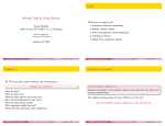
(a)
(b)
Figure 1: Example of title page.
In order to place the university coat of arms in the page background as in
Fig. 1a, the eso-pic package and the following command can be added to the
preamble
\ newcommand \ AlCentroPagina [1]{%
\ A d d To S h ip o u tP i c tu re *{\ AtPageCenter {%
\ makebox (0 ,0){\ includegraphics %
[ width =0.9\ paperwidth ]{#1}}}}}
and then use it as
\ AlCentroPagina { seal_name }
The dots on which to place the signature (Fig. 1b) can be obtained with the
\dotfill command. The titling package allows one to modify the behavior of
6
the \maketitle command. However, the thesis title page is usually so different
from that produced by the standard LATEX classes that it is easier to redefine it
from scratch.
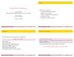
3.2
Dedication
The dedication, when present, can have many different formats depending on the
author’s taste. Usually (Fig. 2) it is just a line aligned to the right which can be
obtained with
\ begin { flushright }
...
\ end { flushright }
The vertical position of the dedication can be arbitrary. An easy way to control
it is with a couple of \vspace{\stretch{...}} commands which let the user
decide the ratio between the space preceding and the one following the line. For
example, in order to set the space following the dedication twice as wide as that
preceding, it is possible to use the command
\ null \ vspace {\ stretch {1}}
...
\ vspace {\ stretch {2}}\ null
3.3
Abstract
The abstract is generated by the environment
\ begin { abstract }
...
\ end { abstract }
which is available for the article and report classes. When using the book class it
is necessary to define the abstract in the preamble (the code that follows is the
definition used by the report class).6
6. Instructions on how to use the fancyhdr package can be found in sec. 6.3.1.
7
Figure 2: Example of dedication.
\ usepackage { fancyhdr }
\ pagestyle { empty }
\ newenvironment { abstract }%
{\ cleardoublepage \ null \ vfill \ begin { center }%
\ bfseries \ abstractname \ end { center }}%
{\ vfill \ null }
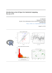
Sometimes it is useful to have the abstract written in two languages. The babel
package can be used to select the correct name of the abstract and the hyphenation. If, for example, you need to write the abstract both in Italian and in English,
you need to load the babel in the preamble with
\ usepackage [ english , italian ]{ babel }
and then use the following commands in the text:
8
(a)
(b)
Figure 3: Example of abstract in two languages.
\ selectlanguage { italian }%
\ begin { abstract }
... versione del sommario in italiano ...
\ end { abstract }
\ selectlanguage { english }%
\ begin { abstract }
... English version of the abstract ...
\ end { abstract }
\ selectlanguage { italian }%
The result is reported in Fig. 3.
9
3.4
Table of contents and other lists
The table of contents and the other lists usually come right after the abstract in
the following order:
– table of contents
– list of figures
– list of tables
– other lists
These are automatically created with LATEX using the commands:
\ tableofcontents
\ listoffigures
\ listoftables
The float package, with the \newfloat and \listof commands, can be used to
create lists of custom floating objects (e.g. programs, algorithms, etc.). The tocloft
package can be used to modify their layout.
3.5
Table of symbols and notation
It is sometimes useful to give the reader a table with the symbols and the notation
used in the thesis (Fig. 4). The nomencl package automatically generates such a
list with the MakeIndex program. It is otherwise possible to manually create the
table with the tabular environment.
3.6
Appendices
The appendices are normal chapters whose numbering is with the Roman alphabet letters. They can be created just by using the \chapter{...} command
preceded by \appendix7 as in the following example:
7. \appendix must be used only once even if there are multiple appendices.
10
Figure 4: Example of a list of symbols.
...
\ mainmatter
\ include { chapter1 }
\ include { chapter2 }
\ include { chapter3 }
\ appendix
\ include { appendix1 }
\ include { appendix2 }
...
3.7
Index
The index can be automatically created with the makeidx package and the MakeIndex program. The \makeindex command must be in the preamble. In order to balance the columns of the last page of the index, it can be inserted into a multicols
environment8 redefining the theindex environment with the following code
\ let \ orgtheindex \ theindex
8. This environment requires the multicol package.
11
\ let \ orgendtheindex \ endtheindex
\ def \ theindex {%
\ def \ twocolumn {\ begin { multicols }{2}}%
\ def \ onecolumn {}%
\ clearpage
\ orgtheindex
}
\ def \ endtheindex {%
\ end { multicols }%
\ orgendtheindex
}
3.8
Bibliography
The bibliography, like the index, can be automatically generated by LATEX. It can
be created with the thebibliography environment, but it is far better to use BibTEX,
a program that allows to separate the content of the bibliography (stored in .bib
databases) and the style (defined by .bst files). The .bib files are just text files
that can be created with any text editor but it is advisable to use bibliography
dedicated editors. JabRef9 is one of the best bibliography managers and, being
based on Java VM, it is available for all platforms (Windows, Linux, and Mac OS
X).
The natbib package is a very useful and flexible tool to format both the bibliography and the references in text as it is thoroughly described in its guide. Every
LATEX distribution and the natbib package offer several bibliography styles; it is,
however, possible to create a custom style. The user just needs to compile the
makebst.tex file and interactively answer the questions. This process creates a
.dbj file that just needs to be compiled with LATEX to produce the .bst style. The
\url{} command provided by the url package automatically breaks long URLs
over several lines. The bibliography can be added to the table of contents with
the \addcontentsline command.
9. http://jabref.sourceforge.net/
12
The following code typesets the references with the plain style, adds the bibliography to the table of contents (for a thesis the bibliography section is a chapter),
and loads the ThesisBib.bib database. The name of the bibliography section is
added to table of contents with the \bibname command in order to let it be dependent on the language used.10
\ cleardoublepage
\ bibli ograph ystyle { plain }
\ refstepcounter { chapter }
\ addcontentsline { toc }{ chapter }{\ bibname }
\ bibliography { ThesisBib }
4
4.1
Objects
Figures
Figures are one of the most popular subject for LATEX guides. There are even
guides and books [3, 9, 23] completely dedicated to this subject. The reader
should refer to them for the details.
LATEX users are usually faced with two kinds of problems regarding the figures. The first kind has its origin in the figure file itself and will be discussed
in sec. 4.1.1, the second kind regards their placement and will be discussed in
sec. 4.3.
4.1.1
Formats
Images can be divided into two big classes: vector images and bitmap images.
The format to use should not be chosen arbitrarily since each one is suitable for
different purposes. The first class, defined as groups of geometric shapes, can be
scaled and deformed without losing definition or sharpness and is recommended
10. \bibname becomes “Bibliography” with the english option, “Bibliografia” with the italian
option.
13
for graphs, schemes and every other image that can be defined in terms of simple
geometric entities. The second class, defined as matrices of colored pixels, cannot
be deformed without altering the information content and should be used only
in cases in which vector graphics are not usable, i.e. for photographs, artistic
paintings, etc.
The conversion between vector and bitmap graphics should always be avoided.
In fact, on the one hand the conversion from vector (e.g. .eps or .pdf) to bitmap
image (e.g. .bmp, .jpg or .png) eliminates all the information on the geometry
contained in the figure and deteriorates the quality of the image and the possibility to resize it without losing any detail. On the other hand, the conversion from
a bitmap to vector graphics does not improve its quality, it just inserts the bitmap
inside a vector frame. The only way to obtain a true vector graphic image from a
bitmap is to trace it with dedicated applications such as Potrace.11
The bounding box is a fundamental parameter of .eps files. It defines the
size of the image and is used by LATEX to compute how much space to assign
to the figure. The bounding box should ideally be the minimum rectangle that
contains the image. Sometimes, however, graphics applications leave margins
(i.e. empty space) between the image and its bounding box. This may cause some
confusion because, although LATEX is assigning to the figure the right space, it
may seem that the figure is too small, not centered, etc. Ghostview12 can be used
to open the figure, visualize the bounding box, and check if the dimensions are
correct. If they are not, the best option is to change settings in the application that
generated the .eps. Alternatively GSView13 can compute the optimal bounding
box14 or the user can directly open the .eps file with a text editor and modify the
values defining the bounding box, which are usually in the first few lines. The
details on how to use figures with PDFLATEX and to convert them from .eps to
.pdf are reported in sec. 5.2.
11. http://potrace.sourceforge.net/
12. http://www.ctan.org/tex-archive/help/Catalogue/entries/ghostscript-afpl.html
13. http://www.ctan.org/tex-archive/help/Catalogue/entries/gsview.html
14. File - PS to EPS - Automatically calculate Bounding Box.
14
4.1.2
Useful packages
The graphicx package needs to be loaded in order to insert figures. Its guide is very
useful.15 Subfigures (Fig. 1) can be obtained with the subfig package.16 In many
cases this package is not even needed since more than one figure or table can be
inserted into a figure or table environment, as shown in the following example
\ begin { figure }[ tb ]
\ includegraphics [ width =0.3\ textwidth ]{ fig : a }
\ caption { caption : a }\ label { fig : a }
\ hspace {4 em }
\ includegraphics [ width =0.3\ textwidth ]{ fig : b }
\ caption { caption : b }\ label { fig : b }
\ end { figure }
This is a good way to reduce the number of floating objects and to facilitate their
placement.
It is advisable to collect all the figures in one or more subfolders to keep the
source files in order. If the fig:a figure is inside the fol_1 folder, the user should
specify it
\ includegraphics { fol_1 / fig : a }
By the way, it is far more convenient to specify the folder’s name just once in the
preamble with the command
\ graphicspath {{ fol_1 /} ,{ fol_2 /}}
The path declared with \graphicspath can be relative to the folder hosting the
main .tex file (as in the previous example), or absolute,17 as, for example,
\ graphicspath {{ c :/ documents / thesis / images /}}
The caption package allows to easily format captions.
15. http://tug.ctan.org/tex-archive/macros/latex/required/graphics/grfguide.pdf
16. This package supersedes the subfigure package, which has been declared obsolete by its own
author.
17. On Linux or UNIX systems the absolute path cannot take advantage of the tilde expansion. For
example \graphicspath{{/home/lapo/documents/thesis/images/}} should be used instead of
\graphicspath{{~/documents/thesis/images/}}.
15
4.2
Tables
The ctable package improves the spacing of the standard tabular environment. The
xcolor package with the table option can be used to color the background or rows,
columns, and cells. When dealing with big tables, it is possible to:
– scale down the table, for example with the following commands:
\ begin { center }
\ resizebox {0.95\ textwidth }{!}{%
\ begin { tabular }
...
\ end { tabular }}
\ end { center }
– rotate the table by 90◦ with the rotating package,18
– break the table over several pages with the supertabular package.
For further details the reader can refer to a specific guide, such as [20].
4.3
Controlling the floating objects
LATEX users often complain about the position of figures (and of floating objects
in general). In most cases this is due to a wrong use of the position options for
the floating objects. This section explains what should be done while writing
(sec. 4.3.1) and what while reviewing the text (sec. 4.3.2).
4.3.1
What to do while writing
First of all the user should accept the fact that LATEX moves a floating object either
because there is no space on a given page or for esthetic reasons. Luckily, when
using the right commands, LATEX does a very good job.
The very first thing to do is to avoid commands like \clearpage and let LATEX
choose automatically the position of the floating objects: while writing the thesis,
18. Other techniques to rotate tables and figures are reported in [28].
16
the author should be focused only on the content and not be concerned about
the layout. Almost any interference in the complex routine that LATEX uses to
place the floats causes the result to be worse. The following suggestions assure
that the floats are placed as close as possible to their insertion point without any
intervention by the author.
One of the major causes of dissatisfaction is the use of the [h] option which
asks LATEX to place the figure at the same point where it appears in the code.
Even worse than [h] are the [htbp] and the [h!t] options. It is common belief
that this option is the best to guarantee that the object remains close to the point
where it appears in the code. It actually works only when the object is very small
(compared to \textheight). The only thing that the author should determine is
whether the object is small enough to appear on a page with other text or will
require a whole page to itself. In the first case the best option is [tb], in the
second [p]. If there are no floats left to place, then in the first case LATEX will
place the object just before its insertion point (which cannot happen when using
[h]) or on the following page. When using the [p] option for big objects, they
will be placed on a separate page right after the insertion point and not at the end
of the chapter as in the case of [tbp]. This is what is done in every book with a
good layout: the figures are either at the top or at the bottom of a page, in a blank
page if very big, and in the text if very small. Some users are annoyed by figures
that precede their reference in the text (e.g. a figure that appears at the top of the
page of its reference in the text). This problem can be easily solved with the flafter
package that prevents the floating object from appearing before its definition in
the text.
In general, LATEX chooses a good place for figures if the ratio
text
figures
is sufficiently high. Thus it is advisable, not only from a typographic point of
view, to write something interesting instead of filling up the thesis with figures.
17
If this ratio is too low, LATEX may produce this error:
! LaTeX Error : Too many unprocessed floats .
This is due to the fact that LATEX can allocate only a limited amount of memory
to place the floating objects. If there are too many floats to be processed, this
amount of memory might be insufficient [5]. This problem can be solved with
the \FloatBarrier command, provided by the placeins package, which cannot be
crossed by floating objects and forces LATEX to place all the ones that are still in
memory. If possible, even the \clearpage command can be used. It inserts a page
break and also places all the unprocessed floats. The morefloats package increases
the number of floats that can be held in memory from 18 to 36. Some journals
require that all the figures are placed at the end of the draft. The endfloat package
does that automatically.
Should all these tricks not be enough, the user can make some manual adjustments just before printing, as explained in the next section.
4.3.2
What to do while reviewing
Just before printing the thesis, it might be necessary to adjust manually the position of some floating objects such as tables and figures. The float package provides the H position option which make the floating objects non-floating and
forces their placement in the exact place in the text. The \FloatBarrier command (see sec. 4.3.1) can even be used to fine tune the position of some objects.
LATEX provides some commands to globally control the floating objects:
\setcounter{topnumber}{...} maximum number of floats in t position for each
page
\def\topfraction{...} maximum page fraction for floats in t position for each
page
\setcounter{bottomnumber}{...} maximum number of floats in b position for
each page
18
\def\bottomfraction{...} maximum page fraction for floats in b position for
each page
\setcounter{totalnumber}{...} maximum number of floats in the same page
\setcounter{dbltopnumber}{...} maximum number of big floats in the same
page
\def\textfraction{...} minimum fraction of the page for the text
\def\floatpagefraction{...} minimum page fraction for floats in p position
for each page
\def\dbltopfraction{...} maximum part of a two-column text page that can
be occupied by two-column floats at the top.
\def\dblfloatpagefraction{...} minimum part of a page that has to be occupied by two column wide floating objects before a ‘float page’ is produced.
5
5.1
Compiling the code
Choosing the format
The LATEX code can be compiled to obtain a DeVice-Independent file (.dvi) or a
Portable Document Format file (.pdf).19 Each format has advantages and disadvantages. On the one hand, the .dvi allows a direct search (with a double click
on the code inside the text editor, the .dvi viewer finds the corresponding output) and inverse search (with a double click on the output inside the .dvi viewer,
the text editor positions the cursor at the corresponding position in the code) that
are very useful when writing the thesis. Unfortunately most .dvi viewers do
not render properly the effects of the graphicx package such as \resizebox and
\rotatebox20 and cannot take advantage of the microtype package (see sec. 5.2).
19. There is actually a third option, the PostScript file (.ps), but it has been substituted by the
.pdf format as the de facto standard.
20. YAP (MiKTEX.dvi viewer) solved this problems since the 2.5 version.
19
The .pdf format, on the other hand, although it does not allow direct and inverse
search,21 renders correctly all the effects of the graphicx package, takes advantage
of the microtype package, is a very popular format even outside the TEX and LATEX
community, takes advantage of the hypertext links of the hyperref package, and
allows to restrict the document access with a password.22
In conclusion, it is recommended to use the .dvi while writing and the .pdf
for printing the thesis and distributing it in electronic format.
5.2
Creating a PDF
There are several ways to create a .pdf with LATEX, such as:
– converting a .dvi or a .ps file with Ghostscript,
– directly compiling the source .tex code with PDFLATEX.
Without going into the details, for which a good reference is [24], in order to
exploit all the potential of the PDF format23 it is necessary to use PDFLATEX which
is available in most LATEX distributions.
The main difference between the two methods is the file format for the figures; while the conversion from .dvi or .ps files requires .eps images, PDFLATEX
requires .pdf (if vector graphics) or .jpg and .png (if bitmap).24 In order to use
PDFLATEX, the user is required to convert all .eps into .pdf files. The conversion can be easily done with Ghostscript by using the graphical user interface
eps2pdf.25 If the document has to be compiled both with LATEX and PDFLATEX it is
21. The MacTeX distribution for Apple computers allows direct and inverse search even with .pdf
files.
22. A password can be used to limit access to the document, to limit the print options (restrict it or
allow it only at low resolution), and to limit changes (text extraction, page extraction or removal,
etc.).
23. The PDF format allows to use hypertext, bookmarks, thumbnails, and document information
which are not available when converting .dvi and .ps files.
24. The details about image format are reported in sec. 4.1.1.
25. eps2pdf is a graphical user interface for Windows and is available on CTAN (http://www.
ctan.org/tex-archive/support/eps2pdf/). Linux users can use the homonymous sh procedure
20
advisable not to specify the extension of the image files in the \includegraphics
command; if, for example, the document has the figure_01.eps image, the user
need to convert it into figure_01.pdf with eps2pdf and then add to the code
\ includegraphics { figure_01 }
In this way, LATEX automatically loads figure_01.eps and PDFLATEX figure_01.pdf.
The hyperref package needs to be loaded in order to create hypertext links in
a document.26 To learn how to use TrueType fonts with TEX (LATEX) and PDFTEX
(PDFLATEX) the reader can visit http://www.radamir.com/tex/ttf-tex.htm. The
microtype package is highly recommended when using PDFLATEX because it improves line filling with:
– font expansion: it horizontally expands the characters in order to optimally
fill each line;
– character protrusion: it let some characters to protrude into the margins (typically the hyphens and punctuation signs).
These two modes are already enabled when the package is loaded without any
options:
\ usepackage { microtype }
6
6.1
Useful packages
Hyphenation
Hyphenation is controlled by the babel package and depends on the active language. If the thesis is in English, the following command should be used
\ usepackage [ english ]{ babel }
or epstopdf (both of them from command prompt). All these programs just use GhostScript to
convert .eps into .pdf.
26. Even some .dvi viewers support hypertext links.
21
The babel package is necessary to have hyphenation but not sufficient: the file
with the hyphenation patterns for the used language should be active (refer to
the documentation of the LATEX distribution used).27 For English the definition
file is hyphen.tex.
LATEX correctly syllabifies almost every English word. However, in some cases,
when using rare words or names, the author might need to suggest the correct
hyphenation with the command \hyphenation in the preamble. The words must
be between curly braces and separated by a space as in the following example
\ hyphenation { hy - phen -a - tion mar - vel - ous - ly }
This command can even be used to force that some words are not syllabified: they
just need to be written without hyphens as in the following example:
\ hyphenation { MATLAB Mathematica }
When a word appears just once or only a few times, it is possible to suggest the
hyphenation directly in the text with the \- command as in the following example
hy \ - phen \ - a \ - tion
The author should always remember that all manual operations on the hyphenation should be done only during the review process immediately before
printing. It is often better to rewrite a sentence that causes an overfull warning
than to impose a certain hyphenation.
6.2
6.2.1
Languages other than English
Indentation
In some languages (e.g. Italian) the first paragraph needs an indentation on the
first line (Fig. 5). This can be easily achieved with the indentfirst package.
27. Here is reported as an example the procedure to activate the hyphen.tex file on MiKTeX: from
the “languages” panel on “MiKTeX options” activate “english – hyphen.tex” and then update the
formats with ”Update Formats” in “General”.
22
(a) without the indentfirst package
(b) with the indentfirst package
Figure 5: Example of indentation on the first paragraph.
23
6.2.2
Accented letters
Accented letters can be inserted into LATEX code with the standard commands28
(\‘{e}, \’{e}, etc.) or directly from the keyboard (è, é, etc.) using the inputenc
package with the appropriate encoding. The inputenc options depend on the
editor that is used. [ansinew] has to be used with most editors on Windows
(e.g. WinEdt and TEXnik Center); [latin1] or [latin9] with most editors on
Linux, UNIX, and Mac OS X; [applemac] with Macintosh computer using an
operating system prior to OS X and even OS X depending on the encoding used
by the editor;29 [utf8x] can be used only on some editors such as on Linux and
TEXShop on Mac OS X.
6.3
6.3.1
The layout
Headers and footers
The fancyhdr package is very useful to customize headers and footers. In a thesis,
headers and footers usually differ from one part to the other. It is convenient to
define commands that change their behavior as in the following example:
\ newcommand {\ fncyfront }{%
\ fancyhead [ RO ]{{\ footnotesize \ rightmark }}
\ fancyfoot [ RO ]{\ thepage }
\ fancyhead [ LE ]{\ footnotesize {\ leftmark }}
\ fancyfoot [ LE ]{\ thepage }
\ fancyhead [ RE , LO ]{}
\ fancyfoot [ C ]{}
\ renewcommand {\ headrulewidth }{0.3 pt }}
\ newcommand {\ fncymain }{%
28. See [22] for a list of these commands.
29. [applemac] corresponds to the MacOSRoman encoding which is used by default by Mac OS
9 and Mac OS X. It is however possible to use other encodings depending on the editor used.
For example TEXShop allows to save files with every encoding (MacOSRoman by default, but
also Latin1, Latin9, Unicode, and all the others). The software deriving from *nix systems on the
Macintosh platform (e.g. Emacs) usually uses the [latin1] encoding.
24
\ fancyhead [ RO ]{{\ footnotesize \ rightmark }}
\ fancyfoot [ RO ]{\ thepage }
\ fancyhead [ LE ]{{\ footnotesize \ leftmark }}
\ fancyfoot [ LE ]{\ thepage }
\ fancyfoot [ C ]{}
\ renewcommand {\ headrulewidth }{0.3 pt }}
These commands are then used in the text as follows:
\ pagestyle { fancy }
\ fncyfront
\ frontmatter
...
\ fncymain
\ mainmatter
The openright class option might cause a blank page at the end of the chapter.
The following command can be added to the preamble to avoid headers and
footers on this blank page:
\ makeatletter
\ def \ cleardoublepage {\ clearpage \ if@twoside
\ ifodd \ c@page
\ else \ hbox {}\ thispagestyle { empty }\ newpage
\ if@twocolumn \ hbox {}\ newpage \ fi \ fi \ fi }
\ makeatother
6.3.2
Page layout
University rules very often require a page layout different from that of the standard LATEX classes. It could be changed using LATEX primitive commands such
as \textwidth, \oddsidemargin, etc., but this is not advisable for several reasons
[5, 26]. A better solution consists in using rigid packages, such as layaureo,30
30. Other packages such as widemargins, a4, and a4wide, could be used to modify the layout but
they are not suggested because they are obsolete.
25
Figure 6: Example of page crop marks.
which are very easy to use31 but do not let the user define the layout. If none
of these rigid packages produces the desired layout, the geometry package, which
is very flexible, is recommended. The chngpage package allows to change single
pages or paragraphs.
In order to bind the thesis it might be convenient to indicate where to cut the
pages (Fig. 6). This can be easily done with the packages geometry and crop.
LATEX tries by default to cover the entire page height and, if necessary, it expands the space between paragraphs, list items, and so on. This behavior can be
disabled with the \raggedbottom command32 which leaves empty space at the
bottom of pages if necessary. In order to improve page coverage it is possible
to let the mathematical display environments break across two pages with the
\allowdisplaybreaks command.
31. The layaureo package provides two layouts (with and without the big option) and allows to
easily set the binding space with the binding command.
32. The default behavior is obtained with the \flushbottom command.
26
6.3.3
Line spacing
University rules often require a line spacing different from single spacing (which
is the LATEX default). There are many ways to modify the line spacing [26] but the
best one is to use the setspace package. It provides three predefined line spacings
with the commands \singlespacing, \onehalfspacing, and \doublespacing. If a
different spacing is required then the \setstretch{baselinestretch} command
can be used in the preamble to set the baselinestretch appropriately.
6.4
6.4.1
The style
Fonts
The T1 encoding, which is the new standard for LATEX, should always be used.
This encoding is not the default yet to guarantee backward compatibility, but can
easily be selected with the command
\ usepackage [ T1 ]{ fontenc }
Some problems, such as fuzzy fonts, might arise when visualizing the PDF [5].
The cm-super font is a simple solution to this problem since it provides a PostScript
Type 1 font with the same shape as cm and tc families with several improvements
such as support for non-ASCII characters.33 In addition, the latin modern family
is a vastly expanded computer modern, with even more support for non-ASCII
characters than cm-super. Further details about this family can be found in its documentation and in [19]. When writing a scientific thesis, it is convenient to load
the amsfonts package, which provides some mathematical fonts by the AMS, and
the amsmath package, which provides several extensions to typeset mathematics.
The relsize package allows to modify the size of the font with relative commands
(\smaller and \larger) in addition to the standard LATEX commands.34
33. http://en.wikipedia.org/wiki/ASCII
34. tiny, scriptsize, footnotesize, small, normalsize, large, Large, LARGE, huge, and Huge.
27
LATEX users who come from the What-You-See-Is-What-You-Get (WYSIWYG)
world,35 at least in the beginning, often wish to change font. This phenomenon
is probably due to the fact that the WYSIWYG software provides such bad topographic output that the disappointed user often tries to improve it changing
the font. I suggest sticking with the LATEX default font family, that is to say the
Computer Modern family which was developed by the very same inventor of TEX,
Donald Knuth. Changing a font with LATEX is not as easy as with a WYSIWYG
editor and for a reason. When changing a font, four families (Serif, Sans-serif,
Typewriter, and mathematical fonts such as A, A, A, and A) which form a good
typographic combination need to be chosen. Moreover, most fonts do not provide
all the mathematical symbols and so can be used just in the text.36 If you do want
to change the font, many packages can be used to change font (e.g. pxfonts, mathpazo, courier, eulervm, literat, lucida, pandora, mathptmx, helvet, courier, kerkis, kmath,
qpxmath, qtxmath). Otherwise it is always possible to manually install a font as it
is accurately explained in [19].
6.4.2
Chapter titles
The fncychap package allows to modify the format of chapter titles. The default
format produced by the book class is reported in Fig. 8 while the command
\ usepackage [ Lenny ]{ fncychap }
was used in Fig. 7.
The quotchap package can also be used to customize the titles, altough it offers
many fewer options than fncychap.
35. http://en.wikipedia.org/wiki/WYSIWYG
36. The Danish TUG hosts a web site that reports all the fonts that support mathematics (http:
//www.tug.dk/FontCatalogue/mathfonts.html) and other informartion can be found in [5].
28
6.4.3
Lists
The enumerate package allows to modify the item numbering of enumerate-like
environments. It can change the counter style37 and the delimiter symbol.38
6.4.4
Minitoc
When the chapters have a very complex structure, it may be convenient to report
a table of contents of the chapter on its first page (Fig. 7). These “minitocs” can
be automatically produced by the minitoc package.
6.4.5
Epigraphs
The epigraph package allows to insert an epigraph in the first page of each chapter.
An example is reported in Fig. 8.
6.4.6
Footnotes
By default, LATEX produces high quality footnotes. When it is really necessary,
however, the user can change the footnote layout with some dedicated packages and commands. The footmisc package provides many options to control
the footnotes, such as bottom which places the footnotes at the bottom of the
page (Fig. 9).39
In order to prevent a single footnote from spreading over several pages, the
user can set a high penalty to this behavior with the command
\ i n t e r f o o t n o t e l i n e p e n a l t y =10000
The part of the page assigned to the footnotes can be controlled with the
command
37. It is possible to use Arabic numerals (1,2,3,. . . ), uppercase (I,II,III,. . . ) and lowercase (i,ii,iii,. . . )
Roman numerals, uppercase (A,B,C,. . . ) and lowercase (a,b,c,. . . ) Roman alphabet letters.
38. Every character can be used as a delimiter obtaining for example 1), 1., 1 –,. . .
39. LATEX by default places the footnotes after the last line of the page thus, when a page is not
fully covered, the footnotes are not at the bottom of the page.
29
Figure 7: Example of a “minitoc”.
\ dimen \ footins =2 cm
6.5
6.5.1
Mathematics
“Special” symbols
“Special” symbols are all the symbols that cannot be typed directly from the keyboard. For the mathematical symbols you should refer to the amssymb package
provided by the AMS. For all the other kinds of symbols there are specific packages that can be easily identified with [22].
30
Figure 8: Example of an epigraph.
6.5.2
Numbers
numprint is a very useful package to represent numbers. Among the other functions provided, it can automatically insert a separator every three figures and
approximate a number. For example,
\ numprint {2.742647826672 E -01}
gives
2,743 · 10−01
6.5.3
Units
To avoid formatting by hand the units, it is advisable to use the SIunits package.
For example
\ unit {32 ,1}{\ micro \ metre }
gives
31
(a) with the bottom option
(b) without the bottom option
Figure 9: Position of the footnotes.
32
32, 1 µm
6.5.4
Other packages
The empheq package can be used to highlight mathematical environments. The
theorem package can be used to customize theorem-like environments. The xfrac
package allows to write fractions in the text and in the mathematics (e.g. 5/7).
6.5.5
System of equations
It is sometimes useful to group a system of equations with a curly brace. A
convenient way to do it is by defining a new environment:
\ newenvironment { sistema }
{\ left \ lbrace \ begin { array }{ @ {} l@ {}}}
{\ end { array }\ right .}
For example the following code
\[\ begin { sistema }
x_1 =\ sigma_b ^2 -\ sigma_a \\
x_2 =\ sigma_a ^2 -\ sigma_b
\ end { sistema }\]
produces
(
x1 = σb2 − σa
x2 = σa2 − σb
Similar results can be obtained with the cases environment provided by the amsmath package.
6.6
Acronyms
Acronyms can be conveniently handled with the acronym package which can automatically generate hypertext links between the acronyms in the text and their
definition in the list of acronyms. An example of a list of acronyms is reported in
Fig. 10.
33
Figure 10: Example of list of acronyms.
6.7
Codes and algorithms
The verbatim package can be used to add pieces of code to the text. The listings
package, which recognizes many computer programming languages, allows a
broader control of the code typographic style. Another alternative is the fancyvrb
package.
The algorithm and algpseudocode packages can be used for the algorithms: the
first one generates floating objects, the second one non-floating objects.
6.8
Cross-references
Sometimes it might be useful to use the \ref and \pageref commands together
to refer to figures and table, especially when there are several pages between the
object and the reference. For this purpose some authors use commands like
\ newcommand {\ fullref }[1]{\ ref {#1} on page ~\ pageref {#1}}
However, it is not possible to know beforehand the position of the object and may
happen that the \pageref refers to the same page. The varioref package defines
34
the \vref command in order to take care of these exceptions. This package works
together with babel to adapt to the language in use. For example
see Fig .~\ vref { f5 }
produces, depending on where is the figure, something like
see Fig. 3.1 on the next page
or
see Fig. 3.1 on page 24
As regards equations, the \eqref{...} command should be used instead of
(\ref{...}). For example
defined in eq .~\ eqref { e2 }
produces
defined in eq. (3.6)
6.9
Reviewing the code
When reviewing the code, it is highly recommended to analyze accurately the
.log file and to use the refcheck and showkeys packages to check how \label
and \ref have been employed in the text. Moreover, the draft option of the
documentclass can be used to highlight with black bands the points where the
text goes out of the margins.
7
Useful websites
In addition to the guides and the manuals cited in the bibliography, the Web
offers several resources to solve problems that might show up while writing a
thesis with LATEX.
Google provides, besides the traditional one,40 a search engine dedicated to
40. http://www.google.com/
35
LATEX.41 The Usenet newsgroup comp.text.tex,42 available also in other languages, contains a lot of information. The Comprehensive TeX Archive Network
(CTAN),43 which hosts most of the TEX and LATEX material available in the Web,
has a powerful search engine. Sarovar44 is a large catalog of packages and programs connected with TEX and LATEX. Among the types of search provided, the
“topical” is particularly useful when you don’t know the name of a package but
you know what it should be able to do.
Many universities and research labs offers guides on LATEX, usually targeted
to beginners. We will just mention here Cambridge University,45 Nottingham
University,46 Helsinki University,47 and Emory University.48 Moreover, David
R. Wilkins released his book Getting Started with LATEX in html format.49
References
[1] American Mathematical Society (2002). AMS-LATEX User’s Guide. URL
ftp://ftp.ams.org/pub/tex/doc/amsmath/amsldoc.pdf.
[2] M. Baudoin (1997). Apprends LATEX! URL http://tex.loria.fr/general/
apprends-latex.pdf.
[3] P. Daly (1998). Graphics and Colour with LATEX. URL http://tex.loria.fr/
graph-pack/grf/grf.pdf.
41. http://directory.google.com/Top/Computers/Software/Typesetting/TeX/LaTeX/
42. http://groups.google.com/group/comp.text.tex
43. http://www.ctan.org/
44. http://texcatalogue.sarovar.org/
45. http://www-h.eng.cam.ac.uk/help/tpl/textprocessing/
46. http://www.cs.nott.ac.uk/TSG/manuals/latex/intro/
47. http://www.physics.helsinki.fi/~tfo_www/instr/latex-guide.html
48. http://www.emerson.emory.edu/services/latex/latex2e/latex2e_toc.html
49. http://www.maths.tcd.ie/~dwilkins/LaTeXPrimer/
36
[4] A. Diller (1999). LATEX Line by Line: Tips and Techniques for Document Processing. John Wiley & Sons, 2nd edition.
[5] R. Fairbairns (2007). The UK TEX FAQ. URL http://www.ctan.org/
tex-archive/help/uk-tex-faq/letterfaq.tex.
[6] S. Fear (2005). Publication quality tables in LATEX. URL http://www.ctan.org/
tex-archive/macros/latex/contrib/booktabs/booktabs.pdf.
[7] P. Flynn (2005). A beginner’s introduction to typesetting with LATEX. URL http:
//ctan.tug.org/tex-archive/info/beginlatex/.
[8] M. Goossens, F. Mittelbach, and A. Samarin (2004). The LATEX Companion.
Addison-Wesley, 2nd edition.
[9] M. Goossens, S. Rahtz, and F. Mittelbach (2007). The LATEX Graphics Companion: Tools and Techniques for Computer Typesetting. Addison-Wesley, 2nd
edition.
[10] G. Grätzer (1999). First Steps in LATEX. Springer Verlag, 1st edition.
[11] G. Grätzer (2007). More Math Into LATEX. Birkhauser, 4th edition.
[12] E. Gregorio (2007). LATEX: Breve guida ai pacchetti di uso più comune. URL
http://profs.sci.univr.it/~gregorio/breveguida.pdf.
[13] J. Hahn (1993). LATEX for Everyone: A Reference Guide and Tutorial for Typesetting Documents Using a Computer. Prentice Hall.
[14] D. Higham and D. Griffiths (1997). Learning LATEX. Society for Industrial
and Applied Mathematics.
[15] ISO 5966 (1982). Documentation – Presentation of scientific and technical reports.
[16] D. Knuth (1984). The TEXbook. Reading, Massachusetts: Addison-Wesley.
37
[17] H. Kopka and P. Daly (1999). A Guide to LATEX – Document Preparation for
Beginners and Advanced Users. Addison-Wesley, 3rd edition.
[18] L. Lamport (1994). LATEX: A Document Preparation System, User’s Guide and
Reference Manual. Addison-Wesley Professional, 2nd edition.
[19] P. Lehman (2004).
The Font Installation Guide.
URL http:
//www.ctan.org/tex-archive/info/Type1fonts/fontinstallationguide/
fontinstallationguide.pdf.
[20] L. F. Mori (2007). Tables in LATEX2ε : packages and methods. The PracTEX
Journal, (4). URL http://www.tug.org/pracjourn/2007-1/mori/mori.pdf.
[21] T. Oetiker, H. Partl, I. Hyna, and E. Schlegl (2007). The (Not So)
Short Introduction to LATEX2ε . URL http://www.ctan.org/get/info/lshort/
english/lshort.pdf.
[22] S. Pakin (2005). The Comprehensive LATEX Symbol List. URL http://www.ctan.
org/tex-archive/info/symbols/comprehensive/symbols-a4.pdf.
[23] K. Reckdahl (2006). Using Imported Graphics in LATEX2ε . URL http://www.
ctan.org/tex-archive/info/epslatex.pdf.
[24] N. Talbot (2004). Creating a PDF document using PDFLATEX. URL http://
theoval.cmp.uea.ac.uk/~nlct/latex/pdfdoc/pdfdoc-a4.pdf.
[25] The Tutorial Team (2000). On-line Tutorial on LATEX. Indian TEX Users Group.
URL http://www.tug.org.in/tutorials.html.
[26] M. Trettin (2007). An essential guide to LATEX2ε usage — Obsolete commands and
packages. URL ftp://ftp.tex.ac.uk/tex-archive/info/l2tabu/english/
l2tabuen.pdf.
[27] H. Voß (2007). Mathmode. URL www.ctan.org/tex-archive/info/math/
voss/mathmode/Mathmode.pdf.
38
[28] H. Voß (2007). Rotating Text, Tabulars and Images. URL http://perce.de/
LaTeX/PDF/rotating.pdf.
39
Journal home page
General information
Submit an item
Download style files
Copyright
Contact us
LaTeX goes with the flow
Jim Hefferon Abstract One advantage of TeX and friends is that they fit naturally into a work flow where there are many tools, each good at its own job. This paper gives an example involving a system for doing class evaluations online. Jim Hefferon is a professor of Mathematics at Saint Michael's College, Colchester, Vermont (USA). He is also the maintainer of the US CTAN site and is a member of the TeX User Group board. You can reach him at 




PDF version of paper
Article source
sphyg.sty
Comment on this paper
Send submission idea to editor
Page generated April 13, 2008 ; TUG home page; search; contact webmaster. http://dw.tug.org/pracjourn/2008-1/hefferon/
The PracTEX Journal, 2008, No. 1
Article revision 2008/03/14
LATEX goes with the flow
Jim Hefferon
Abstract One advantage of TEX and friends is that they fit naturally into a work flow
where there are many tools, each good at its own job. This paper gives an
example involving a system for doing class evaluations online.
My college gives students in every class a chance to provide feedback on that
class. We now use a paper-based form but are looking toward online evaluations.
Some advantages of an online system would be: timeliness (reports for a class
would be available immediately after the feedback period instead of six months
later), flexibility (for instance, data could easily be tracked over time), and customizability (more on this below). So for the institution, all of the bullet points
lead in the same direction.
We’ve had no luck finding a vendor. As one approach, I wrote some scripts.
In my system, called Sphyg, part of the job involved moving the data from the
database to the summary documents. For that, the right tool was LATEX.
1
Sketch of the system
To understand how LATEX fits into its flow, we must first understand the evaluation system.
1.1
Customizing the data in
Each semester’s process starts with an email to the academic Vice President and
to the Department Chairs. This mail has a link to an online form.
For instance, the VP’s form allows the input of questions that will eventually
appear on each evaluation seen by each student in each class in the college. These
questions will appear either at the top of those evaluations or at the bottom.
Similarly, each Chair can enter questions for the courses in their department.
These questions appear either at the top of the forms, below the VP’s questions,
or at the bottom above the VP’s.
Each administrator’s form comes up already filled out with last semester’s
questions. Thus if the administrator does not respond, or makes no changes,
then last semester’s questions will just be reused — this is what will typically
happen.
If they do edit the form then for each question there is a place to write the
text of the question, such as “I learned a great deal in this course.” They also
select among question types, including choose types such as choose-one-to-five,
paragraph answer types, and many others (adding new types is easy). For choose
types they also insert a space for students to make a brief comment.
Next, each instructor gets an email. It has links to a page where the instructor
can add questions to the forms for their classes. One link allows them to put in
questions on each form for any of their students. Other links go to different pages
for each section that the instructor is teaching. That is, evaluation forms can be
customized not only by college, by department, and by instructor, but also by
section. As with the administrators, if an instructor does not respond then Sphyg
uses the questions asked last semester by this instructor on all forms.
Now, with the forms made up, each student gets an email. It links to a page
listing the student’s classes and linking to the evaluations for those classes. Of
course, students can submit at most one evaluation per section.
When the period for evaluations closes, Sphyg generates the reports. Each
instructor gets a summary of all responses, for all questions, from students in
each of their sections. That summary preserves the students’s anonymity.
1.2
Customizing the data out
As described above, the system allows extensive customization of the input. But
the output is customized as well.
Administrators do not get the same reports as instructors. The Vice President’s
report shows only the summaries for institution-wide questions. And, each Department Chair’s report summarizes only the questions for the institution or for
the department. This allows the instructor to ask developmental questions such
as “What could I have done better?” that would not fit in an evaluative context.
2
However, this customization adds complexity to the production of the reports
since they cannot just be forms into which the data is inserted.
2
The LATEX generation
There are many ways to get data out of a database and into a report. Just to name
one, the programming language Perl makes generating plain text reports straightforward. But plain text has shortcomings, such as a lack of graphics capability
and colors, and character encodings can be awkward.
I wanted the reports to be nicer than that, for instance to show bar charts for
choice-type questions. That, and also that everyone can read it, means that the
natural format for the report is PDF. Since direct production of PDF would be
very hard, generating the reports using LATEX makes the most sense.
So Sphyg’s document work flow is: a Python script takes the data from the
database and outputs LATEX source files. These are turned into a report by running them through XELATEX. The variant XELATEX was chosen because it makes
convenient the use of a wider character set.
I wrote a custom .sty file for the reports. That means that less of the LATEX
code is mixed in with the Python.
Here is an example showing part of a page, using some of the sample data.
3
A number of things appear in this sample. For instance, LATEX generates page
headers that change depending on the class section. Also notice that the mean
and standard deviation summary information about responses are given for this
single section, across the department, and across the college. Finally, notice the
optional comment shown with the question summary (here there is just one comment but had there been more they would have been listed in alternate shadings).
An advantage of using LATEX in this work flow is that some of its features
make easy things that might otherwise be quite hard.
One example is that the document style uses the graphicx package to make a
macro to draw the bar charts, as shown in the screenshot above.
Another example of leveraging LATEX is that the report style uses the longtable
package to alternatively shade adjacent comments, and to automatically insert
“(continued on next page)” where appropriate.
Still another example is that the hyperref package makes document navigation
easy. For instance, administrative reports have a table of contents with a link from
the instructor’s name to the first page of the summary for that instructor. There
is also an index with a link to the summary for each section of each course. Those
links are created automatically, obviously.
The final aspect of the reports to note is that they can be quite long. The Vice
President’s report has a summary of all of the college-wide questions, including
students’s optional comments, for each instructor. In the tests using dummy data
this report was over a thousand pages. While that length would be a cause for
worry with some document-handling programs, LATEX has no trouble. Further,
compilation of the document takes less than a minute.
3
Status
Sphyg’s LATEX subsystem performed flawlessly. In particular, for the characters
encountered in testing (only Latin-1 characters), XELATEX had no trouble at all.
The main challenge with the larger project of online evaluations is that students do not fill them out — in one of my experiments the most common return
rate was 0%. A person can reflect on the desirability of collecting responses that
users seem not keen on giving, but at my college there is a mandate to be proactive about feedback. So we need an incentive. One is to only allow students to see
their grades online after they have filled out the evaluation. That is why in the
4
system described above students are sent to a page filled with links: once they
have filled out the evaluation then in the place of the link appears their grade.
For this incentive we must temporarily suppress access to the mechanism that ordinarily allows students to see their transcript online. At the moment the online
evaluation initiative is stalled at this point (our online-transcript vendor wants a
great deal of money). In short, whether Sphyg will ever get running is unclear.
What is clear, however, is that LATEX fits well into this kind of flow. For example, if I had instead tried writing the PDF directly from the database then graphics
and pagination would be quite a problem. Instead, with TEX and friends, it was
a solved problem.
5
Journal home page
General information
Submit an item
Download style files
Copyright
Contact us
Learning To Sweave in APA Style
Ista Zahn Abstract Until recently I used MS Word and clones such as OpenOffice to write academic manuscripts, as do most in my field. The standard software toolkit for many psychology professors and graduate students also includes SPSS for performing statistical analyses, and perhaps EndNote or similar reference manager software for generating bibliographies. These tools work, but my experience suggests that LaTeX based solutions have signicant advantages. This article describes how to use Sweave to write LaTeX documents in APA style, complete with results, tables, and figures generated by R. Ista Zahn is a graduate student in the Department of Clinical and Social Sciences in Psychology at the University of Rochester in Rochester, NY. He started using LaTeX during the Summer of 2007 to typeset equations for use in powerpoint lectures, and now uses LaTeX to write scientific articles, presentations, and even posters. He has benefited greatly from the wealth of freely available information about LaTeX available on the World Wide Web, and has recently started work on a manual describing the use of LaTeX and R (an open source statistical programming environment), as a way of giving back to the community. You can reach Ista at . 


PDF version of paper
Comment on this paper
Send submission idea to editor
Page generated April 13, 2008 ; TUG home page; search; contact webmaster. http://dw.tug.org/pracjourn/2008-1/zahn/
The PracTEX Journal, 2008, No. 1
Article revision 2008/4/4
Learning to Sweave in APA Style
Ista Zahn
Email [email protected]
Address University of Rochester
Clinical and Social Sciences in Psychology
Meliora Hall
Rochester, NY 14627
Abstract
Until recently I used Micorsoft Word and clones such as OpenOffice to write
academic manuscripts, as do most in my field. The standard software toolkit
for many psychology professors and graduate students also includes SPSS
for performing statistical analyses, and perhaps EndNote or similar reference
manager software for generating bibliographies. These tools work, but my
experience suggests that LATEX based solutions have significant advantages.
This article describes how to use Sweave to write LATEX documents in APA
style, complete with results, tables, and figures generated by R.
1 Why I made the switch to LATEX and R
I am the only person in my department who uses LATEX and R. Because Sweave1
simply provides a way to integrate these two programs, it follows that I am the only
Sweave user as well. Why have I taken the time and effort to learn these programs
instead of following the crowd and sticking with Word and SPSS? Quite simply, I
made the switch because using LATEX and R is actually easier. It took me some time
to become familiar with these programs, but after using them for a couple of months
I am firmly convinced that I am more productive with these programs than I ever
was with Word and SPSS.
1.1 Advantages to using LATEX and R
There are a number of major advantages to using LATEX and R rather than Word and
SPSS. For example, LATEX users who need to write documents in APA style can use
1. R is an open-source implementation of the S statistical programming language. Sweave stands
for ‘S-weave’, i.e., weaving S code and results into a LATEX document.
This work is licensed under the Creative Commons Attribution-Noncommercial-Share Alike 3.0
United States License. To view a copy of this license, visit creativecommons.org.
apa.cls[6] to completely specify the final appearance of the document. Unlike the
writer using Word, the LATEX user does not need to manually set page numbers, figure
out where to place the running head, affiliation information etc. The LATEX user does
not even need to fiddle with the style of the headings. This is one especially irritating
aspect of APA style; because the headings used differ depending on the number of
headings, one must alter headings throughout the document if the number of heading
levels is changed. With LATEX these details are handled by the computer, allowing
the author to (almost) forget about formatting and concentrate on the content of
the article. There are additional advantages to using LATEX was well, such as the
ability to easily create indexed .pdf files that can be navigated using free PDF viewers
like Acrobat Reader, and the ability to easily create reference lists without manual
formatting.
When used together with R, the LATEX document becomes an almost self-contained
environment in which the author can perform statistical analyses, present the results
in standard APA style, compose the prose of the article, and create and display tables
and figures. All of these activities can take place within a single computer program
(your favorite text editor), reducing distractions and facilitating complete immersion
in the writing process. This article documents some of my experiences using LATEX
and R, and highlights some of the features I find most useful, including automatic
formatting of title pages and section headers, the creation of tables and figures, cross
referencing, and the generation of APA style reference lists.
LATEX and R are both wonderful tools in their own right. LATEX is a powerful,
flexible, and free alternative to the more standard what you-see-is-what-you-get approach to document creation, such as taken by Microsoft Word and OpenOffice. R
is a powerful, extremely flexible, and free tool for performing statistical analyses and
computations. It can replace costly alternatives such as SPSS or STATA, and can
easily handle the relatively simple analyses I need to perform, including analysis of
variance, multiple regression, and structural equation modeling. Sweave is a system
that brings these two wonderful tools together. A Sweave document is basically a
LATEX document interspersed with R code.
1.2 Disadvantages to using LATEX and R
Unfortunately, there are also drawbacks to using LATEX. The most serious drawback
I have encountered is that it can be difficult to collaborate with colleagues who do
2
not use LATEX. Those unfamiliar with LATEX are unlikely to appreciate being sent a
LATEX file, and it can be difficult to convert LATEX files to a format Word can read. If
your collaborators (or perhaps more importantly, journal editors) won’t accept LATEX
documents, you are going to have to figure out a way to do this conversion. I provide
instructions for how to do this in Section 6.
The main disadvantage to using R is the startup cost in terms of learning the
syntax. There are graphical user interfaces available (such as R Commander[2]), but
generally speaking, if you want to use R you are going to have to learn to write R
commands. In my case it took about two months to become comfortable enough with
R to let my SPSS license lapse.
2 Formatting your document in APA style
Because I need to write documents in APA style, I am extremely fond of the APA
document class[6]. Although this article is primarily about Sweave, I’m going to take
a moment to highlight some of the features of this of apa.cls that I find most useful.
To use apa.cls, write \documentclass[man]{apa} in your preamble. This will cause
your document to be typeset in APA manuscript style. If you want to see approximately what the published article will look like, you can use the journal mode by
replacing [man] with [jou] .
2.1 Multiple authors and affiliations
apa.cls supports multiple authors by defining the commands author, twoauthors, and
so on, up to sixauthors. For example, if you have three authors, specify the author
information as follows:
\ threeauthors { F i r s t Author }{ Second Author }{ Third Author }
If you specify multiple authors, you must specify an affiliation for each of them. For
the example above, you could specify
\ t h r e e a f f i l i a t i o n s { I n s t i t u t i o n A}{ I n s t i t u t i o n B}{ I n s t i t u d i o n C}
You can specify up to six affiliations.
Note that some mixing-and-matching is possible here, and that the actual limit
is six affiliations rather than six authors. For example, the following is perfectly
reasonable:
3
\twoauthors{ F i r s t Author }{ Second Author and Third Author }
\ t w o a f f i l i a t i o n s { A f f i l i a t i o n o f F i r s t Author }{ A f f i l i a t i o n o f Second and Third Authors }
and will result in the affiliation of the first author being typeset below the first author’s
name, and the affiliation of the second and third author’s being typeset below their
names.
2.2 Title and header information
There are a total of four title and header related fields that can be specified. Note
that if you do not specify all the fields the information from the fields you do specify
will be used in place of the missing fields. The four fields are:
\ t i t l e {}
\ s h o r t t i t l e {}
\ rightheader {}
\ leftheader {}
Note that there is some possibility for confusion here, as these commands are labeled
according the where the information will go in the published version of the paper
and not in the manuscript version. Thus the shorttitle command actually contains the
information that will go in the right header of the manuscript, while the \rightheader
command contains the information that will be printed as the running head in the
manuscript. The \leftheader command contains information to be printed in the left
header of the published manuscript (usually the author’s name) and is not used in
manuscript mode. Finally, the \title command contains the full title of the article.
2.3 Headings and heading levels
The APA manual specifies different heading styles depending on the total number of
headings in a manuscript. In order for LATEX to figure out how to set your headings,
you therefore need to tell it how many headings you have. This is done by issuing
the \headinglevels{} command in your preamble. Note that the number of headings is
specified by verbal rather than numeric arguments. Thus if your manuscript has four
headings, you need to issue the command \headinglevels{four}, not \headinglevels{4}. The
manual specifies heading schemes for up to five heading levels.
Once you have specified the number of heading levels in the preamble, you issue
section commands as follows:
\ section {}
\ subsection {}
4
\ subsubsection {}
\paragraph{}
\subparagraph{}
Note that all of these may or may not be used, depending on the number of headings.
For example, if you have only three heading levels, you should use only the \section,
\subsection, and \subsubsection headings. If you decide to change the number of heading
levels, LATEX will automatically adjust the appearance of the headings appropriately.
2.4 Enumeration and seriation
Itemized and enumerated lists can appear in APA style manuscripts, but their use is
not common. To create bulleted or numbered lists you can simply use the standard
itemize and enumerate environments. More commonly in APA style documents, one
wishes to have itemized lists that appear in the body of the text, like (a) this, (b) that,
and (c) the other thing. This can be accomplished using the seriate environment, as in
\begin{seriate} \item this, \item that, and \item the other thing \end{seriate} and has the advantage
of being automatically relabeled if you change the order.
2.5 Cross-references, in-text citations, and reference lists
Cross referencing in LATEX is easy and very useful. Basic cross referencing can be
implemented using just two commands. In order to refer to something later on in
your document, you need to give it a label, as in \label{ex:label}. Then you can refer
to it by it’s label, as in \ref{ex:label}. This is especially useful for tables and figures,
because if you change the order, the in-text references to them will automatically be
updated. You can also label sections, equations, and footnotes.
For citations, apa.cls uses the apacite package, which makes formatting citations a very easy process. For the most part, citations in APA style should be very
familiar to BibTEX users. For example, assuming I have an entry for the present work
in my .bib file with the cite-key Zahn2008, I can cite it by writing \cite{Zahn2008}. This
will result in (Zahn, 2008) appearing in the text of the document, and the reference
will be automatically inserted into the reference list at the end of the document. For
details on the apacite package, refer to the manual[5].
Using BibTEX is very simple, and it works great. I’ve used several different
reference management software, and found most of them to be complicated and/or
buggy. BibTEX on the other hand is easy to use and it just works.
5
3 Installing and setting up Sweave
The preceding sections focused on features of LATEX that I find particularly useful. In
this section, I show how the usefulness of LATEX can be further enhanced by combining
it with R.
The documentation accompanying R and various LATEX distributions covers the
installation and configuration of these programs quite well, and so I will not discuss
their installation here. However, having these programs installed and working properly is a pre-requisite for setting up Sweave, so make sure you have both working on
your computer before following the instructions below2 .
I prefer to run Sweave from within a text editor (I use TextMate on OS X),
and therefore these instructions are geared towards setting things up this way. If
you prefer to run Sweave from the command line, simply disregard the parts about
configuring your text editor.
3.1 Setting up Sweave on a Windows computer
In the following I assume you are using TEXmaker with the MikTEX distribution
of LATEX, but the general procedure should be very similar with alternative LATEX
distributions/front ends.
Sweave comes with the standard distribution of R, and can be run from within
the R program without any additional configuration. However, I prefer to run Sweave
directly (i.e., from outside of R), and this requires a few extra steps. First, you will
need to install a batch file3 so you can call Sweave from your text editor. To install
the file, you can either place it somewhere in your PATH, or simply place it anywhere
you like and add the directory to your PATH.
At this point you should be able to run Sweave from the command line. If you
prefer to call it directly from within your text editor, you will need to tell your
text editor where to find the sweave.bat file. Open TEXmaker, and select Edit →
Preferences. Next, select a function you won’t need (I recommend DVI viewer),
replace the command with sweave.bat −−pdf %.Rnw, and click OK.
2. I am currently working on a complete Sweave guide that (among other things) details the
installation and set up of Sweave assuming no previous experience with either LATEXor R. Please
contact me at the e-mail address listed at the beginning of this document to obtain this guide.
3. You can download the file from http://cran.r-project.org/contrib/extra/batchfiles/.
6
On Windows, it is common to encounter difficulties because LATEX cannot find
the Sweave.sty file. To correct this, copy the sweave.sty file from C:\Program
Files\R\R-2.6.2\share\texmf and paste it somewhere your LATEXprogram can
find it.
3.2 Setting up a Sweave on Mac OS X
The procedures involved in setting up a Mac OS X workstation are even easier
than those required for setting up a Windows workstation. If you want to be
able to call Sweave outside of R, you will need to install a shell script4 . To install the script, copy it to /usr/local/bin, then open the Terminal program and
type sudo chmod +x /usr/local/bin/Sweave.sh to make it executable.
At this point you should be able to call Sweave from the command line. If you
want to call Sweave from within TEXshop you need to tell TEXShop where to find the
Sweave.sh shell script. Open TEXShop and click TEXShop → Preferences. Click the
Misc tab and type /usr/local/bin/Sweave.sh −ld in the LaTeX Progam Personal Script
field.
3.3 Setting up Sweave on Linux
The procedures involved in setting up a Linux workstation are also very straightforward, although the details will vary depending on which distribution and text editor
you are using. The present example is based on Kubuntu Linux, using Kile.
If you want to be able to call Sweave outside of R, you will need to install a shell
script (see footnote 4). To install the script, copy it to /usr/local/bin, then open
the Konsole program and type sudo chmod +x /usr/local/bin/Sweave.sh to make it executable.
Next, you may want to tell Kile where to find the Sweave.sh shell script. Open
Kile and click Settings → Configure Kile. Click the Tools tab on the left-hand
side of the preferences window, and select Build. Click the New Tool button at the
bottom of the preferences window. Name the new tool Sweave, click next, and then
Finish. In the resulting screen, type Sweave.sh in the top box, and −ld `\%source' in the
bottom box.
4. You can download the Sweave.sh script from http://cran.r-project.org/contrib/extra/scripts/.
7
4 Sweave basics
In this section I give an overview of and basic introduction to Sweave. As you will soon
find, it is not difficult to learn, but it does require that you have some knowledge
of both R and LATEX. To create a Sweave document, simply set up your LATEX
preamble as usual, use the Sweave package, and save the file with a .Rnw extension.
For example, the first two lines of the present article read
\documentclass{ p r a c j o u r n }
\usepackage{ Sweave }
and the file is named LearningToSweaveAPAStyle.Rnw.
4.1 What happens when you run Sweave?
When you run Sweave, the output is a regular LATEX file, with the R code and
results included. If you have your system set up as described above, this is all hidden
from view, because the program is set up to automatically run LATEX on the Sweave
output. But what looks like a single seamless process is actually a two-stage affair.
This is useful in an important way, namely that we can run Sweave, and then edit
the resulting .tex file to make any manual changes we wish to the results returned
from R.
4.2 Details about Sweave syntax
Unlike LATEX and R, Sweave is not extensive or complicated. This is because Sweave
has a relatively simple purpose: it allows you to combine LATEX and R code into a
single document. The basic Sweave syntax consists simply of a << >>= marker indicating that we want to begin an R code section, followed by one or more R commands,
followed by a @ marker indicating you are done writing R commands and wish to
switch back to LATEX. Although this basic syntax is extremely simple, it’s actually
slightly more complicated than this, because you can put option commands inside the
openning marker. In the following, I discuss only a few of the more commonly used
options; for a full description the available options, see the Sweave user manual[4].
In the examples that follow, I use a simple contrived data set that takes the
following form:
<<echo=f a l s e >>=
P a r t i c i p a n t <− c ( 1 , 2 , 3 , 4 , 5 , 6 , 7 , 8 , 9 , 1 0 )
8
C o n d i t i o n <− f a c t o r ( c ( 1 , 1 , 1 , 1 , 1 , 2 , 2 , 2 , 2 , 2 ) )
S c o r e <− c ( 4 , 3 , 5 , 4 , 4 , 2 , 2 , 6 , 5 , 6 )
Data <− data . frame ( P a r t i c i p a n t , C o n d i t i o n , S c o r e )
Data
@
These R commands create the following simple data frame:
1
2
3
4
5
6
7
8
9
10
Participant Condition Score
1
1
4
2
1
3
3
1
5
4
1
4
5
1
4
6
2
2
7
2
2
8
2
6
9
2
5
10
2
6
If you don’t understand what these commands are doing, make sure to consult an
introductory R guide5 before proceeding.
4.3 The echo option
The echo option dictates whether the R input is incorporated into the typeset document. For example, if we want to calculate the grand mean of the Score variable for
the Data dataset created above, we could say
<<echo=t r u e >>=
mean( S c o r e )
@
which gives us
> mean(Score)
[1] 4.1
or, we could say
<<echo=f a l s e >>=
mean( S c o r e )
@
which gives
[1] 4.1
Notice that in the first case the command returned both the command and the result,
while in the second case only the result appears.
5. Many excellent and free guides are available at http://www.r-project.org/.
9
4.4 The results option
The results option tells Sweave how we want the results formatted. We can hide the
results completely, as in
<<echo=f a l s e , r e s u l t s=hi de>>=
mean( S c o r e )
@
We can return the results already formated in LATEX code (useful especially when we
have R create LATEX tables for us; more on this later), as in
<<echo=f a l s e , r e s u l t s=tex>>=
mean( S c o r e )
@
or we can have the result returned verbatim (the default), as in
<<echo=f a l s e , r e s u l t s=verbatim>>=
mean( S c o r e )
@
The reader is encouraged to play around with these options in order to see what they
do first-hand.
5 Including results from R into your document
The main purpose of Sweave is to allow you to perform statistical analyses and include
the results directly into your LATEX document, without the need to switch programs,
copy-and-paste, or re-type results. In this section I provide examples illustrating
how to do this. Many of the examples use the Prestige dataset from the car[1]
R package. The Prestige data set contains six variables, as described in: the car
package documentation:
education Average education of occupational incumbents, years, in 1971.
income Average income of incumbents, dollars, in 1971.
women Percentage of incumbents who are women.
prestige Pineo-Porter prestige score for occupation, from a social survey conducted in the mid-1960s.
census Canadian Census occupational code.
type Type of occupation. A factor with levels (note: out of order): bc, Blue
Collar; prof, Professional, Managerial, and Technical; wc, White Collar.
In the following I’ll present a number of examples using these data. First, I
illustrate how to calculate statistics and included them in the text of you document.
10
Next, I’ll show you how to make R create LATEX tables for you. Finally, I’ll show you
how to create graphics in R and incorporate them into your LATEX document.
5.1 Incorporating R results using the Sexpr command
There is another way to insert short chunks of R code into your LATEX document.
Quite simply, you can issue the \Sexpr{} command, and put your R code inside the
brackets.
For example, if I say \Sexpr{2+2} I will get 4. The nice thing about this command
is that the indexes (i.e., those pesky [1] ’s peppered throughout the examples above)
are automatically suppressed, and the result is returned in the same font as the rest
of the normal text in your document.
The \Sexpr command can be very useful. Instead of copying and pasting results
from SPSS into Word, we can do all our calculations right in our LATEX document.
Here is a brief example:
The average income was
\Sexpr{mean(income)}, with a standard deviation of \Sexpr{sd(income)}.
The average level of education was
\Sexpr{mean(education)}, with a standard deviation of
\Sexpr{sd(education)}. The correlation between income and education was
\Sexpr{cor(income,education)}.
This will be typeset as:
The mean income was 6798, with a standard deviation
of 4246. The mean level of education was 11, with a
standard deviation of 2.7. The correlation between
income and education was 0.58.
Once I got used to reporting results this way, it’s hard for me to imagine how
I ever worked without it. It’s so simple, so easy, that I can’t help but wonder why
anyone would go to all the trouble of having separate interfaces to their statistical
and document preparation software. And it gets even better with Sweave, as we can
do exactly the same kind of operations with tables and figures that we just did with
single values.
11
5.2 Including tables in your document with xtable
There are two separate R libraries that can be used to create LATEX tables in R.
The first is the xtable package[8], which was designed exclusively for this purpose.
The other is the Hmisc package[3], which includes the latex () command. I’m going to
illustrate the use of xtable because I’ve found it easier to use. xtable formats table
results in LATEX style, turning the utilitarian R output into nicely formated tables.
To load the xtable package, simply write library(xtable) inside a Sweave tag.
Once the libraries are loaded, you are almost ready to begin making tables. To
make a table of descriptive statistics we need to do a bit of work in R before calling
xtable. Specifically, we need our descriptive statistics to be formatted in a data frame,
after which we can run xtable on the data frame. Here is an example that creates a
table displaying descriptive statistics for the income and education variables found
in the Prestige dataset:
<<echo=f a l s e , r e s u l t s=tex>>=
means <− c (mean( income ) , mean( e d u c a t i o n ) )
s d s <− c ( sd ( income ) , sd ( e d u c a t i o n ) )
mins <− c (min( income ) , min( e d u c a t i o n ) )
maxs <− c (max( income ) , max( e d u c a t i o n ) )
d e s c r i p t i v e s <− data . frame ( means , sds , mins , maxs ,
row . names =c ( ”Income ” , ”Educa t i o n ” ) )
names( d e s c r i p t i v e s ) <− c ( ”Mean ” , ”SD” , ”Min ” , ”Max” )
d e s c r i p t i v e s . table <− x t a b l e ( d e s c r i p t i v e s , c a p t i o n =
” D e s c r i p t i v e S t a t i s t i c s ” , l a b e l = ”tab : d e s c r i p t i v e 2 ” )
print ( d e s c r i p t i v e s . table , i n c l u d e . rownames=TRUE)
This will produce the result displayed in Table 1.
Table 1: Descriptive Statistics
Mean
SD
Min
Max
Income 6797.90 4245.92 611.00 25879.00
Education
10.74
2.73
6.38
15.97
The xtable package also has extensive methods for creating tables displaying the
results of inferential statistics. For example, we can create an ANOVA table summarizing the results of a linear regression model predicting income from education, as
follows:
<<echo=f a l s e , r e s u l t s=h i de>>=
library ( x t a b l e )
12
x t a b l e ( anova (lm( income ˜ e d u c a t i o n ) ) , c a p t i o n =
”ANOVA Table ” , l a b e l= ”tab : a n o v a t a b l e 1 ” )
@
The results are displayed in Table 2. This basic method can be applied to just about
any model object. About the only thing that you might object to is the somewhat
unconventional labels used across the top of the table. It is possible to modify these
values in the model object before calling xtable, but I find that this is often more trouble
than it’s worth, and I’m usually better off just using xtable to get an approximate result
of what I want, and then tweaking the table (by editing the LATEX file that Sweave
produces) to get the details right.
Table 2: ANOVA Table
Df
Sum Sq
Mean Sq F value
education
1.00 607421386.02 607421386.02
50.06
Residuals 100.00 1213392025.00 12133920.25
Pr(>F)
0.00
To do this, simply open up the file, and find the table generated by xtable. In
the present case, we find
% l a t e x t a b l e g e n e r a t e d i n R 2 . 6 . 2 by x t a b l e 1.5 − 2 p a c k a g e
% F r i Mar 28 1 3 : 0 2 : 5 6 2008
\ begin { table } [ ht ]
\ begin { c e n t e r }
\ caption {ANOVA Table }
\ l a b e l { tab : a n o v a t a b l e 1 }
\ begin { t a b u l a r }{ l r r r r r }
\ hline
& Df & Sum Sq & Mean Sq & F v a l u e & Pr ( $>$F) \\
\ hline
e d u c a t i o n & 1 & 6 0 7 4 2 1 3 8 6 . 0 2 & 6 0 7 4 2 1 3 8 6 . 0 2 & 5 0 . 0 6 & 0 . 0 0 0 0 \\
R e s i d u a l s & 100 & 1 2 1 3 3 9 2 0 2 5 . 0 0 & 1 2 1 3 3 9 2 0 . 2 5 & & \\
\ hline
\end{ t a b u l a r }
\end{ c e n t e r }
\end{ table }
Now all we need to do is edit the table to make it look exactly like we want it to,
and re-typeset the document.
13
5.3 Graphics in Sweave documents
The beauty of Sweave is that we can use R to create the graphics, and include the
results all from a single, unified, and consistent interface (i.e., our text editor). In the
following sections, I will walk you through a way of doing exactly this. R comes with
robust plotting capabilities, and there are several add-on packages that extend these
capabilities. I’m going to use the ggplot2 package[7] in the following examples, but
the general procedure should work even if you use another plotting package.
To generate a figure, we simply place the required R code inside the <<>> = ... @
tags. There are actually a few different ways to go about inserting the figure. The
method I’m going to present here is specifically chosen because it makes it easier to
produce figures that are sized appropriately, with appropriately sized axis labels and
legends (something that can be tricky with other methods). Specifically, I recommend
creating your graphic and saving it to a .pdf file, and then inserting the image into a
figure environment. For example, we can easily represent the relations among income,
education, type of occupation, percentage of woman in a field, and the prestige of
a field, all in one information-dense graphic. The code for doing all this is simply
<<echo=f a l s e , r e s u l t s=hi de>>=
p d f ( f i l e=” s p l o t 1 2 . p d f ” , width =6 , h e i g h t =5)
q p l o t ( e d u c a t i o n , income , shape=type , s i z e=women , c o l o u r=p r e s t i g e ,
x l a b=”Edu ca t i o n ” , y l a b=”Income ” )
dev . o f f ( )
@
\ begin { f i g u r e }
\ centering
\ i n c l u d e g r a p h i c s [ width=6in , h e i g h t =5 i n ] { s p l o t 1 2 . p d f }
\ caption {A s c a t t e r p l o t d i s p l a y i n g t h e r e l a t i o n s h i p s
among Income , Education , P r e s t i g e , Type o f o c c u p a t i o n ,
and p e r c e n t a g e o f Women i n t h e f i e l d . }
\ label { f i g : f i g 1 2 }
\end{ f i g u r e }
The result is displayed in Figure 1, and really shows off the impressive capabilities of
qplot() .
The R command pdf() tells R to save the graph to a .pdf file. Then we include
the graph with the standard \includegraphics []{} command making sure to specify the
same size in the options as we did in the options to the pdf() command. Note that the
pdf() command expects the units to be in inches, so just write the number of inches
you want, while the \includegraphics []{} command needs to be told that the values are in
inches (i.e., write \includegraphics[width = 3in]{file} rather than just \includegraphics[width=3]{file},
which will make LATEX complain that you didn’t tell it what to do).
14
Type
●
25000
bc
prof
wc
Women
Income
20000
15000
●
0
●
20
●
40
● 60
●
80
prestige
10000
●
●
●
●
●
●
5000
●
●
●
●
●
●
●
●
● ● ●
●
●
●●
●
●●
●
●
20
●
30
●
40
●
50
●
60
●
70
●
80
●
●
● ●
●
●
●
●
●
●
●
●
●●
●
●
●
●
8
10
12
14
Education
Figure 1: A scatterplot displaying the relationships among Income, Education, Prestige, Type of occupation, and percentage of Women in the field.
6 Collaborating with those who don’t use Sweave
One of the most frustrating things about learning to use Sweave is that it can be
difficult to collaborate with colleagues who do not. A related concern is that journals
will not accept articles in LATEX format. Both of these are valid concerns. They can
be worked around, but in my experience there is no completely satisfying solution.
There are a number of programs that can convert simple LATEX files to .rtf
or .html, both of which can be read by most word processors, including Microsoft
15
Word. Such programs include latex2rtf and latex2html, and others6 . Unfortunately,
my experience is that such converters do not handle APA formated LATEX documents
well, if they can even be coaxed into producing any output at all.
As strange as it sounds, my advice is to forget about converting your LATEX document to a Word-readable file directly. Instead, typeset the document as a .pdf file,
and then convert the .pdf file to .html (.html files can be read by most modern
word processors, including Microsoft Word). There are stand-alone conversion programs that will do this for you, such as the excellent pdftohtml7 . If you have Gmail
you can send the .pdf document to yourself, and click the View as HTML button in
the Gmail web interface. Finally, Adobe has an on-line converter8 that can convert
.pdf’s to .html, although this can be slow for long documents. Once you have the
.html formated document, open it in your word processor and fix the formatting
(which will usually be close but not exactly right), and save it in .doc format.
The conversion to .doc format will usually be easier if you set your LATEX document to left-justified (aka ‘ragged right’; \raggedright), and if the margin settings
in LATEX match the margin settings in your word processor. If you use apa.cls in
manuscript mode you shouldn’t have too much trouble.
7 Conclusions and final thoughts
The preceding sections document some of the things I’ve learned to do with LATEX
and R. Some sections descended into detailed discussions of various techniques, taking
us a long way from the general, largely personal tone of the opening section. In this
final section, I want to step back from the discussion of specific techniques, and offer
my personal thoughts about using Sweave.
In the summer of 2006, I was looking for a calculator program for OS X. I had
trouble finding one I liked, and eventually started using R as a simple calculator. I
can almost hear the R developers shrieking in horror to think that someone would
use their powerful and sophisticated program as a calculator, but the truth is that
R serves this function very well. As time went on, I started using R for analysis of
variance and linear regression as well. Over the course of several months, I gradually
began using R more and more, and SPSS less and less.
6. A list of conversion programs is available at http://www.tug.org/utilities/texconv/textopc.html
7. Available at http://sourceforge.net/projects/pdftohtml/
8. Available at http://www.adobe.com/products/acrobat/access onlinetools.html
16
In the summer of 2007, I taught an introductory statistics course. I needed to
prepare lecture slides that included a lot of math, and Google pointed me towards
LATEXit, a small OS X program for typesetting math, based on LATEX. I was so
impressed with LATEXit, that I started teaching myself to use LATEX. It didn’t take
long for me to find out about Sweave, and since that time I’ve used LATEXand R for
all my papers, as well as my presentations (using the Beamer package).
In this way, I found myself using tools that are completely different from those
used by the majority of my colleagues, and different from the tools I’ve learned to
use since grade school. In general, my impressions so far are that (a) LATEX is both
easier to use and produces better output than Word, and (b) R is easier to use and
produces better output that SPSS. Of course neither of those statements were true
when I first started. Indeed, I almost gave up on R at one point because it seemed
more difficult than SPSS. But once I took a few months to learn it, it became quite
natural and easy to use.
Overall then, I am quite happy to be the only one in my department using LATEX
and R. I don’t have to pay expensive licensing fees, and I get to take advantage of all
the wonderful features of LATEX and friends. In addition, I’ve learned how to convert
.pdf’s to .html, which means I can still collaborate effectively with Word users, and
I can always convert my documents before submitting them for publication if I have
to. In sum, my experience with LATEXand R have been very rewarding. I hope that
by sharing these experiences and giving a few pointers I have inspired you to give
Sweave a try.
References
[1] John Fox. car: Companion to Applied Regression, 2007. R package version 1.2-7.
I am grateful to many people for various suggestions and contributions.
[2] John Fox and with contributions from many others. Rcmdr: R Commander, 2008.
R package version 1.3-12.
[3] Frank E Harrell Jr and with contributions from many other users. Hmisc: Harrell
Miscellaneous, 2007.
[4] Friedrich Leisch. Sweave User Manual, 2007.
17
[5] Erik Meijer. The apacite package: Citation and reference list with LATEX and
BibT EX according to the rules of the American Psychological Association, 2005.
[6] Athanassios Protopapas. APA LaTex Class File, 1.3.2 edition, 2006.
[7] Hadley Wickham. The ggplot book, 2007.
[8] David B. Dahl with contributions from many others. xtable: Export tables to
LaTeX or HTML, 2007. R package version 1.5-2.
18
Journal home page
General information
Submit an item
Download style files
Copyright
Contact us
Using BiBTeX to produce customized layouts
Yogeshwarsing Calleecharan Abstract Normal LaTeX and TeX usage does not require touching existing .bst files nor creating new ones. However, BibTeX offers several interesting commands which can be used to do many things apart bibliography generation. In this article, it is demonstrated how customized layouts for a database can be created without much trouble. Yogeshwarsing Calleecharan can be reached at . 





PDF version of paper
datab.bst
datab.bib
datab.tex
Comment on this paper
Send submission idea to editor
Page generated April 13, 2008 ; TUG home page; search; contact webmaster. http://dw.tug.org/pracjourn/2008-1/calleecharan/
For submission to The PracTEX Journal
Article revision 2008/02/07
Using BiBTeX to produce customized layouts
Yogeshwarsing Calleecharan
Email [email protected]
Abstract Normal LATEX and TEX usage does not require touching existing .bst
files nor creating new ones. However, BibTEX offers several interesting
commands which can be used to do many things apart bibliography generation. In this article, it is demonstrated how customized layouts for a
database can be created without much trouble.
1 Introduction
To many LATEX users, BibTEX and its commands remain a mystery. Yet as pointed
out in [1], LATEX users can play with BibTEX commands and use it for purposes
other than bibliography generation. Since I started using LATEX in 2005, I realized
that handling LATEX and TEX as programming languages can really make one
abandon traditional word processing packages as the sky certainly becomes the
limit.
The article [1] is regarded as the most exhaustive source of information on BibTEX.
BibTEX is a powerful tool for handling a database and in this article, I have a
modest goal: To show how BibTEX can be used to create customized layouts for
a database. I am sure that any LATEX user will be able to create more interesting
layouts given here and to adapt them for their own needs.
2 A Simple Example
Programming books often begin their first program with the traditional words
Hello World! displayed on the screen. We shall remain faithful to this tradition
and use BibTEX to this end. By displaying just two words, the codes shown
next serve to outline the minimal structure of a .bst file which is the key file in
creating any desired style or layout.
Copyright © 2008 Yogeshwarsing Calleecharan.
No part of this publication may be copied or reproduced
without obtaining permission from the author through email.
Normally where a .bib file is involved, it is useful to run the minimal commands: LATEX BibTEX LATEX LATEX in succession. I use the TEXMAKER [2] IDE to
do the compilation and the IDE built-in Quick Build tool permits constructions
of macro-like commands that save button presses. Further time can be saved
by giving the same filename to the .tex, .bib and .bst files as in first.tex,
first.bib and first.bst as this allows running the Quick Build tool on any of
these files.
Enough of talking now! Displaying the words Hello World! has nothing to do
with formatting a database of information but it can be useful to illustrate the
structure of a .bst style file. For a database one would normally start with the
.bib file and think of the fields required for different entry types. But here for
this simple example, we directly create the .bst file as one entry is enough to
display Hello World!. We will need to create three files: first.bst, first.bib
and first.tex. Next is shown the first.bst file listing:
1
2
3
4
5
6
7
8
9
10
11
12
13
14
15
16
ENTRY
{ toDisplay
} {} {}
FUNCTION{print}
{
cite$ pop$
}
FUNCTION{style1}{
print toDisplay write$
}
FUNCTION {fin}
{newline$
}
READ
ITERATE{call.type$}
EXECUTE {fin}
We shall give a short attempt to dissect the first.bst file listing and detailed
information of the commands used are available in [1]. We begin on line 1 with
the BibTEX ENTRY command which is used to create a field named toDisplay
2
which will be defined later in the first.bib file. The two pairs of matching
braces on line 3 are for internal variables and will not be discussed further. The
next important command is FUNCTION. All the macro functions in our example are
user-defined. Furthermore, a function can also be made to run via the EXECUTE
command (refer to line 16).
The FUNCTION command takes as first argument the name of the function and as
second argument its definition which usually contains a useful sequence of instructions. On line 9 we find the internal command write$ which interprets the
sequence of instructions between the function argument name print and itself
on the same line, and it writes the output in a .bbl file, which is generated on
running BibTEX. On line 4 is the first function called print which will pop out
the topmost item from the stack via the pop$ command. The user can change
the argument name print on line 4 to anything that he or she likes e.g. rambo
provided the same argument name is written on line 9 as well. But as in programming, it is always better to work with meaningful names. Finally, the other
important function is on line 8 and it takes as first argument style1 and defines
the sequence of instructions on line 9 as second argument. This function also
defines an entry type (style1) which shall appear in the first.bib file as well.
Moving further down in the file listing first.bst to line 14 is the READ command
which is advisable to be placed after all functions have been defined. Occurring
just once in a .bst file, it processes only from the first.bib file the entries listed
in the first.aux file (generated on LATEX compilation). Next on line 15 is the
ITERATE command which should come after the READ command. This command
is executed for a number of times that equals to the number of entries in the
first.bib file (subject that an entry is called in the first.tex file). In this first
example, there is just one entry as will be seen later in the file first.bib. The
ITERATE command has as argument call.type$ which looks for the name of each
entry to be executed in the first.bib file and takes this name as argument. And
this call.type$ command works together with the cite$ on line 6 to treat each
entry in the first.bib file in turn.
Finally on line 16 is the EXECUTE command which is required to generate an
output from a .bst file. It has been found necessary to add an arbitrary function
named fin (with newline$ as argument) so that BibTEX compiles correctly. The
newline$ command begins a new line.
3
The next step is to write the .bib file where one entry is sufficient to display
the words Hello World!. Thus we will have the entry type style1 defined in
first.bst, a key named arbitrarily as Elem1 and then one field named toDisplay
taking as argument the words Hello World!. The listing of the first.bib file is:
@style1{Elem1,
toDisplay = {Hello World!}
}
1
2
3
In last we write the first.tex file. Omitting for brevity the compulsory \documentclass
commands and the document environment, the listing of the .tex file is:
1
2
3
\nocite{Elem1}
\bibliographystyle{first}
\bibliography{first}
We should note two things here. Firstly, the \nocite command is used instead
of the usual \cite for bibliography generation. The interested reader can try the
latter command to see why \nocite is better. Secondly, since we have created
a custom .bst file whose objective is not principally for bibliography generation, we choose the bibliographystyle and the bibliography to be the style file
first.bst.
After running LATEX for the first time, .aux and .log files are generated. Then,
running BibTEX yields .bbl and .blg files, and finally a run with LATEX twice
again gives the .dvi file with the words Hello World! displayed. There is
nonetheless one serious drawback to use BibTEX as we have been showing. Most
of the time, the user will make a BibTEX related error in the .bib and .bst files. In
this case, BibTEX will only complain of undefined citation(s). During compilation,
many files are created and the TeXMAKER [2] IDE offers a tool to clean these
compilation-time files except for the .blg file. This is a convenient feature that
allows to isolate the .tex, .bib and .bst files quickly and hence investigate any
mistake(s).
4
3 A Database Example
Table 1 shows a few entries of a tiny database which contains some information
on the first three elements of the Periodic Table. We will see how BibTEX may be
used to create a custom layout to present the data in Table 1 in a different way.
Here unlike in our first example, we will first identify the fields from Table 1 and
thus create the .bib file. There are five fields namely: Atomic Number, Element,
Symbol, Type and Group. The second line from Table 1 concerning the element
Helium for instance is converted to a bib entry as shown next.
Table 1. First Three Elements in the Periodic Table
Atomic #
Element
Symbol
Type
Group
1
Hydrogen
H
Nonmetal
I
2
Helium
He
Noble gas
VIII
3
Lithium
Li
Alkali metal
I
1
2
3
4
5
6
7
8
@style2{Elem2,
atomicNumber = {2},
name = {Helium},
symbol = {He},
type = {noble gas},
group = {VIII},
note = {A very light gas}
}
We have taken the liberty to add a field named note in the style2 function and
it will become useful in Section 4.1. The next file to write is the .bst file and
here we will concentrate on writing the style2 function. The reader is referred
to the available file datab.bst which contains this function. The style2 function
is given next:
5
1
2
3
4
5
6
7
8
9
10
11
FUNCTION{style2}{
" {\bf " write$ print atomicNumber write$ " }" write$%
print "{ \kern-2.6mm}" write$ ". " write$ name write$%
", " write$ symbol write$ newline$ newline$
print "\\" write$ " It is classified as " write$ type write$%
" and is found in group " write$ group write$%
newline$ newline$
print "\\" write$ " {\sl " write$ "Note: " write$%
newline$ print note write$ " }" write$
print "\\" write$
print "\\" write$
In the style2 function, the symbol % denotes that the successive line does not
start a new line but instead continues just afterwards. In essence there are just
five lines (with formatting commands) starting on line numbers 2, 5, 8, 10 and 11
respectively and they act as second argument to the style2 function. More will
be said on the formatting techniques used in Section 3.1. The final step is to write
the .tex file. Here we have three entries corresponding to the three elements
of Table 1 and as in the previous section, the entries can be outputted through
\nocite{Elem1}, \nocite{Elem2} and \nocite{Elem3} respectively. The output
for instance from a .dvi file, if a dvi viewer has been called, is shown in Fig. 1.
Figure 1. Customized layout 1 obtained with style2.
Two things are noteworthy here. Firstly, one is free to output the information that
is desired. This can be achieved in two ways. Commenting the whole of line 8
6
of the style2 function in the .bst file listing would prevent the note field from
being outputted. Inserting the % symbol (normally after write$) in the style2
function enables one to control which information is to be outputted. This is a
huge convenience in getting desired information from a database. That said, the
attention of the reader is drawn to the verbatim style2 function listed where the
% symbols have only been included so as the listing can fit within the text width
of this article.
A second method is to extract only specific entries by choosing which of the
three entries from Table 1 is to be outputted. This can be easily be done in
two easy ways: Either the entry to be hidden is commented in the .tex file as
%\nocite{Elem3} for the key entry of Elem3 for instance (defined in the .bib file)
or the entry in question is modified by removing the @ symbol appearing in front
of the key entry in the .bib file. This feature helps the user to pick out which
entry that he or she needs. This issue will be re-visited with the final example in
Section 4.
3.1 Formatting Techniques
In this subsection, we will focus a bit on the formatting used in the previous
.bst file listing. Formatting with BibTEX commands bears resemblance to those
of LATEX but there are some new commands like write$ and newline$ which have
to be inserted at the right places. The print function plays a central role here. It
has the effect to get something outputted after compilation. For example, the sequence of instructions print " It is classified as " write$ will output the
line It is classified as and typing print type write$ as on line 9 will output
the type of the element as per Table 1.
If more complex formatting is desired as shown on line 2, the following sequence
of instructions
" {\bf " write$ print atomicNumber write$ " }" write$
will write the atomicNumber in bold. Finally, the newline$ command is a native
BibTEX that functions as the newline \n command in C programming. However,
newline$ on its own might not suffice and it has been found that two newline$
commands, one after the other, will force BibTEX to move to a new line. If an
7
empty line is to be inserted, then the sequence of instructions on line 10 will do
the job.
3.2 Taking It A Bit Further
In the same .bst file (datab.bst), the user can define another function say style3
that produces a different formatting from that of the style2 function. Considering more elements in the Periodic Table, a user can choose between style2 and
style3 the formatting style that he or she would like to apply to an individual
element (and its associated information like Atomic Number etc.). Now it might
be a good idea also to have the possibility to group the elements pertaining to one
formatting style under a heading or title. But what if the information outputted
spans more than a page? Then it will be convenient to have the relevant headings
at the beginning of each page. This issue will be covered in the next section.
4 An Elaborate Example
This section aims to combine some various features of BibTEX commands so as
to give the reader a bigger perspective of what can be done. We will still work
with the Periodic Table. Since formatting with BibTEX can be trickier than LATEX,
it should be noted that the examples given only serve to introduce the capabilities
of BibTEX and as such these examples only offer basic formatting techniques that
do not necessarily comply with typographic conventions.
Essentially, two features will be demonstrated and the codes accompanying the
discussions are available. Briefly the two features are as follows: Firstly, it will be
shown how to add another function which will give a different formatting style
to other entries. In addition the function will be created in a manner so that it
will have the possibility to filter out a field (which is note in our case) when it is
empty. Secondly, a different layout in the form of a table will be created and as
in the first case, we shall see how we can take advantage of table properties from
a LATEX package.
8
4.1 Filtering Out An Irrelevant Field
Referring to Fig. 1 in Section 3, we see that unlike the elements Helium and
Lithium, Hydrogen has an note field. Say that a user would not like BibTEX to
output a blank note field as he or she considers it to be a waste of space. Besides, say the user would not like information contained within the field group
for the element to be displayed. In this case, one has to write another function
say style3. This new function can be included in the same .bst file (datab.bst)
containing the function style2 listed in Section 3. Also one might want to include headings in the output file so that the two styles style2 and style3 can
be distinguished from each other. To our rescue, there is the well-established
longtable [3] package.
We will start with putting headings in our style files. The longtable [3] package
offers a convenient feature to have a table spanning the full width of a page
via the commands \setlength\LTleft{0pt} and \setlength\LTright{0pt}. A
function arbitrarily named createsection containing mostly commands from the
longtable [3] package permits headings to be created and classification (and
demarcation) of entries (refer to the datab.bib file attached). One can further
make use of commands like \endfirsthead and \endhead for better structure.
The next thing that we shall investigate is how to display the note field only when
this field in the .bib file is not empty. To this end, we shall make use of the BibTEX
commands if$ and empty$. The if$ internal command, like in programming
languages, allows decisions subject to some defined conditions while the empty$
command elegantly fits our specific need here as in combination with an if$
command, it allows an output to be written or not. The output from the style3
function is shown in Fig. 2 and the reader is invited to compare this figure to
Fig. 1 from Section 3. The reader is also directed to [1] for deeper insights.
Headings do not accompany Fig. 2 in order to save space but the user is reminded
again that the createsection function is responsible for the headings and also
commands like the key environment %\nocite{begcla1} and %\nocite{endcla1}
are required (refer to the file datab.tex).
9
Figure 2. Customized layout 2 obtained with style3.
4.2 Yet Another Formatting Style
The objective here is to create a tabular structure like Table 1 but this time displaying only three fields: Atomic Number, Element and Symbol. The function is
named style4 and by making use of the longtable [3], running headings can
be easily made for example when a table continues to a new page. The function
tablesection given in the attached datab.bst file handles the headings in this
case. It contains only some basic formatting and a user can easily bring modifications.
5 Some Useful Information
The user is referred to the datab.bib and datab.tex files where entry types
(style2, style 3 and style4) or styles are grouped under argument key environment such as begcla2 and endcla2. The user is invited to mix styles under
a given argument key environment.
Nevertheless, BibTEX is stubborn in that it will not allow a key (referring here
to elements Elem1, Elem2 etc. as in the datab.bib file) to be repeated. A simple
workaround would be to give the duplicate key a different name (as under the
tablesection function in the datab.bib file) and to adjust the corresponding
entries in the .tex file accordingly.
10
6 Conclusion
By writing this article, I hope that more LATEX (and TEX) users will be encouraged
to consider digging into BibTEX commands. BibTEX is a well-suited tool to handle static database information. The user is expected to realize that almost any
information which can be treated as a database can benefit from the formatting
techniques shown.
Readers conversant with the Extensible Markup Language (XML) will find that
BibTEX perhaps is not as flexible in terms of simplicity and capabilities. But let us
remind ourselves of two important things: Firstly, BibTEX and XML were created
for different purposes, and secondly BibTEX has been here before XML came to
life. Hence, any comparison is unfounded and unfair.
That said, this gap can lessened if BibTEX is combined with JabRef [4] to unveil similar XML capabilities like filtering, sorting and information retrieval [5].
JabRef [4] is a very flexible tool where the user can create custom fields and maybe
through custom filters, it can produce better results than given in this article. I
will not venture in this alley as tweaking deep with JabRef [4] remains a mystery
for me.
Nevertheless, even without JabRef [4], smart constructs can be made with BibTEX
as we have seen in Section 4 with commands like if$ and empty$. With the sky
being the limit for LATEX, TEX fans, who knows how BibTEX will spice up our
world in the future?
Disclaimer
The codes available with this article are named datab.tex, datab.bib and datab.bst
respectively. Compilation is achieved through running LATEX BibTEX LATEX LATEX
sequentially. No guarantee is made for the accuracy of the information contained
in the database nor the codes provided are warranted to be fit for any particular
application.
11
References
[1] Nicolas Markey. Tame the Beast: The B to X of BibTeX, Version 1.3, October
2005.
[2] TeXMAKER 1.2.1. 2004-2005, http://www.xm1math.net/texmaker/.
[3] David Carlisle. The longtable Package, CTAN: http://www.ctan.org/texarchive/help/catalogue/entries/longtable.html.
[4] JabRef Reference Manager 2.3.1. 2008, http://jabref.sourceforge.net/.
[5] Michael J. Young. Formation Á XML. Microsoft Press, 2000, Translated to
French from English: James Guerin.
12
Journal home page
General information
Submit an item
Download style files
Copyright
Contact us
Travels in TeX Land: Another ornament for "thought breaks"
David Walden Abstract In this column in each issue I muse on my wanderings around the TeX world. In this issue I touch again on a topic from my column in TPJ 2005-4 -- another ornament to use for "thought breaks." David Walden is retired after a career as an engineer, engineering manager, and general manager involved with research and development of computer and other high tech systems. More information is available at www.walden-family-com. He may be contacted at . A complete list of his "travels in TeX Land" pieces is at http://www.walden-family.com/dave/index.htm#travels-in-texland. 





PDF version of paper
two-half-ornaments.jpg
half-ornament.mp
yuri.mp
Comment on this paper
Send submission idea to editor
Page generated April 13, 2008 ; TUG home page; search; contact webmaster. http://dw.tug.org/pracjourn/2008-1/walden/
The PracTEX Journal, 2008, No. 1
Article revision 2008/02/20
Travels in TEX Land: Another ornament for
“thought breaks”
David Walden
Abstract In this column in each issue I muse on my wanderings around the TEX
world. I suggested at the end of section 2 of my last column that I would
continue my investigation of colors and TEX in this issue. However, I was
distracted for much of the period between issues by a health problem (now
resolved). Thus, in this issue I only have time to touch briefly again on a topic
from my column in TPJ 2005-4 — another ornament to use for ”thought
breaks.”
Another ornament to use with “thought breaks”
Before reading the rest of this column, you might look up my column in issue
2005-4 and read section 4 on “thought breaks”: http://www.tug.org/pracjourn/
2005-4/walden/. You might also look at Steve Peter’s piece in the same issue on
“swelled rules”: http://www.tug.org/pracjourn/2005-4/peter/.
In the previous column I began using the words “thought breaks” to describe
those points in the text of a book or article where a new train of thought begins
without there being a section or subsection title. Such breaks are often indicated
by some extra vertical space and some sort of ornament or by some extra vertical
space and perhaps a different font face for a character, few characters, or few
words, as shown at the beginning of the following paragraph (this particular
style of thought break, including the seemingly odd half line indent, is used in
the U.S. hardback edition of Robertson Davies’ book The Cunning Man, published
by Viking in 1994).
During my health situation, I spent
some of my time reading The Book of Salt by Monique Truong. I read the paperback edition from the “A Mariner Book” imprint of Houghton Mifflin Company
Copyright © 2008 David Walden
(Boston and New York) that was first published in 2004. This book used an ornament to indicate thought breaks (see page 36, for example) that I greatly admire.
Thus, I thought I would try to replicate it . . .
. . . in some way that allowed me to use it with TEX.
The easiest thing is to scan the ornament, clean it up a bit with Photoshop,
and access it as a graphic, e.g.,
\noindent\hfil\scalebox{.12}
{\includegraphics{salt-ornament-alone-3.jpg}}\hfil
which results in the following.
That looks pretty good (especially on the printed page — print it out). Blown up
about eight times, it looks like this:
But those little imperfections aren’t really visible in the size I would use it in a
book, as shown above.
However, I thought that it might be “more pure” to somehow recreate the
ornament in METAFONT, MetaPost, or some LATEX graphics package.
At this point, I got to chatting (via email) with issue editor, Yuri Robbers.
He noted three possibilities that came to mind for him for creating the desired
graphic:
2
1. using a large print on graph paper and hand coding the outline of the ornament
2. using autotrace and pstoedit
3. from MetaPost to METAFONT or an otherwise usable glyph or font
First approach
The first approach had already come to mind before I talked with Yuri. As Yuri
noted, this was the approach used by Donald Knuth, and described in his Digital
Typography book, to develop his early fonts and also used by Knuth with Zapf
to develop the Euler Math Fonts. However, the 600 dpi scan I have would still
need to be blown up by a factor of four or more to be big enough to measure
and hand code its coordinates, but at that magnification it no longer is made up
of smooth curves and straight lines — rather, it’s made up of lots of pixels that
would require lots of interpolation, e.g., using a French curve to draw the outline.
Second approach
The second approach had immediate appeal because it sounded like a program
would do the tracing for me, as described by Karl Berry in “Making outline
fonts from bitmap images,” TUGboat, Volume 22 (2001), Number 4, pp. 281-295,
which Yuri pointed me to. So, I downloaded an already-compiled Windows version of the autotrace program from http://autotrace.sourceforge.net/, unzipped it into a folder autotrace, opened salt-ornament-alone-3.jpg with Photoshop, saved it as a bitmapped file, salt-ornament-alone-3.bmp in the directory
autotrace, read the README file a tiny bit, and gave the command
./autotrace.exe --output-format eps --output-file out.eps salt-ornament-alone.bmp
This ran to completion but produced the following file (blown up so you can
see the details)
3
which is not usable. But it is sort of amazing that it managed to find the outline at
all. To make autotrace do what I wanted was maybe going to take more reading
of the options described in the README file.
But, before taking the big step of reading and understanding the autotrace
man page (all the documentation it has, apparently), I decided to first bash ahead
and see if a better scan of the ornament would help. I rescanned the ornament
at 2400dpi (4 times more resolution than the first scan had) and specified for the
scanner to directly output a bitmap image (rather than outputting a JPG which
I later converted to a bitmap using Photoshop), and specified B&W rather than
color (I had scanned the earlier image in color and later converted it to B&W in
Photoshop). This resulted in approximately the following image
which has a few white spots and some non-smooth corners but looked pretty
good. So I tried autotrace again, which resulted in the following as an EPS or
PDF file.
That’s only slightly worse than the scan — which still leaves me sort of impressed with that capabilities of autotrace. But, of course, I could have just
converted my improved bitmap to EPS or PDF with Photoshop and skipped using autotrace, so it was actually not much help in my situation versus just using
4
the scan itself with \includegraphics embedded in a new LATEX command such
as \dropinornament.
See also the Appendix.
Third approach
Thus, it seemed like it was time to try Yuri’s third suggestion — trying to figure
out some curves in MetaPost, for instance, that approximate the desired ornament.
I looked at the documentation in the Graphics Companion for a few minutes
and got discouraged about figuring out how to find the points to generate splines,
Bézier curves, etc. (like many or perhaps most people, I have a pretty short attention span for reading documentation). So I looked again at the high resolution
scan of the previous section, this time with Illustrator. With Illustrator it was
pretty easy to select the pen tool, touch points approximately on the outline of
the scan (fuzzy though it was at the edges), and read the X-Y coordinates of the
pen position from Illustrator’s GUI display.
Thus, I collected points along the top half of the left half of the ornament. I
put these into Excel, thinking that I would use Excel to create a reflected set of
points with which to draw the bottom half of the left half of the ornament. In
the end, I didn’t need Excel for this, but it was handy to have the points in Excel
for converting all of the points to positions where both their X and Y coordinates
were positive (MetaPost apparently didn’t like points with negative X values that
I had recorded from the images position in Illustrator).
I next looked up how to use MetaPost to draw a set of connecting curves from
point by looking at the first 20 or so pages of Hans Hagen’s MetaFun manual
(www.pragma-ade.com/general/manuals/metafun-p.pdf). I tried one small test
using his instructions on page 9 for running MetaPost directly, but immediately
switched over to running ConTEXt’s texexec, as also described on page 9, so I
could easily go straight to a PDF without having to run Adobe’s Distiller. (Of
course, I could also have looked at MetaPost output using MiKTEX’s YAP displayer of DVI files.)
It took me at least an extra hour to get all the X-Y coordinates typed correctly
into my text editor (just using the scan directly is looking better all the time).
Here is what I fed into MetaPost via texexec:
5
\starttext
\startuseMPgraphic{dummy}
path p;
p := (1,145)..
(4,156.5)..
(13.5,162.5)..
(27.5,164)..
(42,163)..
(55.5,160)..
(68.5,155)..
(83,149)..
(92,150)..
(96,160.5)..
(91,170)..
(86,182.5)..
(82.5,198.5)..
(84,207.5)..
(89,211.5)..
(96,211.5)..
(102,205)..
(107,193.5)..
(115,183)..
(125,172)..
(136.5,163.5)..
(155,155.5)..
(171.5,152)..
(187,150)..
(208.5,149.5)..
(221.5,148.5)..
(228,148.333)..
(233.167,148.5)..
(234.833,148.5)..
(235,149.667)..
(234.167,150.667)..
(230,151.883)..
6
(223.167,155)..
(212.833,161.333)..
(204.833,167.333)..
(199.5,175)..
(198.167,182.333)..
(199.833,186.667)..
(203.167,189.667)..
(208.167,189.667)..
(210.833,187)..
(216.5,180.667)..
(225.5,173.333)..
(233.833,168)..
(241.167,166)..
(251.167,164)..
(258.833,162.667)..
(267.167,161.333)..
(274.5,160.333)..
(284.167,160)..
(293.5,159)..
(304.5,158)..
(313.167,155.667)..
(317.833,153.667)..
(321.167,151)..
(322.5,145.667)..
(322.5,145)--cycle);
fill p withcolor black;
draw p;
path q;
q := p reflectedabout((0,145),(335,145));
fill q withcolor black;
draw q;
\stopuseMPgraphic
\useMPgraphic{dummy}
\stoptext
7
I learned about filling a closed cycle by glancing at Troy Henderson’s “A beginner’s guide to MetaPost for creating high-quality graphics” (http://www.ursoswald.
ch/metapost/tutorial.html). I learned about creating the bottom half of the left
half of the ornament by reflection in MetaPost from the same few pages at the
beginning of Hans’ manual.1
The figure produced by the above MetaPost code is the following, which I
converted into a JPG so I could include it here using includegraphics:
Obviously at this point I could have tuned up some of the coordinates in my
MetaPost file to eliminate slight imperfections in the ornament. However, when
the ornament is reduced to the appropriate size for use in a book or paper, I doubt
these imperfections will show, and so I will not bother trying to make things more
perfect.
Now I suppose I need to learn how to give a name to the above drawing in
my MetaPost code and then rotate it about a vertical axis to get the other half of
the ornament. And I also suppose I need to learn to input the Postscript from
MetaPost into LATEX file. However, it really is easy to just copy the half ornament
in Photoshop, rotate it, paste the rotated copy, and save the pair of half-ornaments
as a graphic, e.g.,
which I can insert into any text file by defining a macro with the appropriate
scaling and with an appropriate name, e.g., into a thoughtbreak macro such as I
illustrated in my 2005-4 column:
\newcommand{\thoughtbreak}{\vskip2pt
1. You can get the file itself, half-ornament.mp, from the HTML page for this column.
8
\centerline{\scalebox{.05}{\includegraphics{two-half-ornaments.jpg}}}
\vskip2pt\noindent{}}
This looks pretty good compared with the scan from the book on page 2, so
I think I’ll end this column now. The graphic for this ornament is in the file
two-half-ornaments.jpg which can be accessed via this column’s HTML page.
Postscript
The 2008 Major League Baseball season is about to start, and the Red Sox Annual
2008 from Maple Street Press (Hanover, MA) has been published and uses the
following ornament for its thought breaks.
I love it.
Addendum
After I thought I was finished with this column, I received an email from Aditya
Mahajan who had read the column on the journal’s staging website before this
issue was officially posted for public viewing. He said, “I do not understand
why, ultimately, you are using the ornament as a jpg. Since you have created the
ornament from MetaPost, you can simply include either a pdf or eps into your
document. That way, you retain the advantage of having the ornament as a vector
graphic. A jpg is a bitmap format and will not look good when zoomed in; the
pdf/eps format will look good even when zoomed in.
“Since you are using MetaPost inside ConTEXt, you can just say
\starttext
\startMPpage
metapost code
9
\stopMPpage
\stoptext
and you will get a pdf whose page size is same as the size of the ornament.”
There were two reasons why I used a jpg. First, I only created half the ornament in MetaPost, and it was easier for me to use Photoshop to create the other
half of the ornament and save the two halves as a jpg than it was to learn how
to create the other half of the ornament using some symmetry operation in MetaPost. Second, I did not know how to get a PDF page which was only as big as the
ornament when included as a graphic; Aditya Mahajan’s set of commands above
apparently solves that problem.
Appendix — Yuri’s experiment with autotrace
After reading the subsection on my efforts with the second approach, Yuri Robbers tried the second approach himself using my 2400dpi scan. He cleaned up
the scanned image using Gimp (the free equivalent of me using Photoshop) and
then ran autotrace. The autotrace processing created the file yuri.mp, which in
turn was converted into an EPS file which produce the following image:
His result is not quite as good as my result from using the third approach, but it
is obviously a pretty good result.
The content of Yuri’s MetaPost file (yuri.mp) can be seen by looking at the
link on the HTML page for this column.
10
Acknowledgments
Issue editor Yuri Robbers provided editorial and editing help and other guidance
and ideas. Karl Berry caught several typos and made other useful suggestions.
Biographical note
David Walden is retired after a career as an engineer, engineering manager, and
general manager involved with research and development of computer and other
high tech systems. He holds an undergraduate math degree and completed a
graduate school sequence of courses in computer science. More history is at
www.walden-family.com/dave.
11
Journal home page
General information
Submit an item
Download style files
Copyright
Contact us
Ask Nelly: How do I create math mode columns in tabular environments? How do I find the files required to compile my document? The Editors Abstract Ask Nelly is a question and answer column. Nelly is the quiet person who sits at the back corner desk, who knows a lot, and when asked any question is always ready with a patient answer. If Nelly doesn't know the answer, Nelly will know an expert who has the answer. Feel free to Ask Nelly
about any aspect of LaTeX, TeX, Context, etc. 

Comment on this paper
Send submission idea to editor
Q: Dear Nelly: When I create tables with columns for which each and every cell contains mathematical content, I keep on switching into and out of Math mode all the time. Surely there is a better way to do this? A: There is indeed! Frank Mittelbach and David Carlisle, names probably not unfamiliar to you, have solved this problem for you with their wonderful array package. This package, among many other things, redefines the tabular environment in such a way that it allows you to already declare mathematical mode when defining your table, so instead of — for example — using \begin{tabular}{lll}
when you want all three columns to just contain material to be typeset in math mode anyway, you could use \begin{tabular}{>{\(}l<{\)}>{\(}l<{\)}>{\(}l<{\)}}
which creates a table with three left aligned columns, all three of which are to contain mathematical content. Should you want to create many such tables in your document, array even allows you to define new column types to make your life easier still. To define the mathematical equivalents of the three standard column types, just use \newcolumntype{L}{>{\(}l<{\)}}
\newcolumntype{C}{>{\(}c<{\)}}
\newcolumntype{R}{>{\(}r<{\)}}
and then whenever you need to create a three column table with three left-aligned columns containing mathematical http://dw.tug.org/pracjourn/2008-1/asknelly/
contents all you need to do is \begin{tabular}{LLL}
Although remember to use \multicolumn to change a cell back to regular type if you need non-mathematical information in a cell, as is often the case in, for example, column headings. An example, assuming the new column types having been defined as explained above: \begin{tabular}{LLL}
\hline
\multicolumn{1}{l}{Function}&\multicolumn{1}{l}{Derivative}&\multicolumn{1}{l}{Primitive}\\
\hline
ax^n & nax^{n-1} & \frac{1}{n+1}ax^{n+1} + C\\
\sin(x) & \cos(x) & -\cos(x) + C\\
\cos(x) & -\sin(x) & \sin(x) + C\\
\hline
\end{tabular}
The above question was answered by Yuri Robbers, a member of the editorial board of this journal. He can be reached at Q: Dear Nelly: When I tried to co-author a paper, I ran into trouble because my colleague did not have some of the files needed to properly compile the document. I am aware of the \listfiles directive, which can be added to the preamble in order to get a list of files included by LaTeX. In some cases, however, when trying to locate these files on my system I find multiple versions (Yes, I know, I should take better care of my system, but there you have it!). Is there a way to get the file list with the full path to each file? A: The problem here is that the TeX engine is not actually aware of path names. Luckily, there is a way around this. If you use the option -recorder with tex, latex, pdflatex etc. you will get a file with extension .fls that contains every file opened for input as well as output, including their pathnames. As an example I did a LaTeX run on a tiny example file, as follows: pdflatex -recorder centaurtestje
And the resulting file centaurtestje.fls has the following contents: PWD /home/yuri/texmf/knoeien
INPUT /home/yuri/.texlive2007/texmf-var/web2c/pdftex/pdflatex.fmt
INPUT centaurtestje.tex
OUTPUT centaurtestje.log
INPUT /usr/local/texlive/2007/texmf-dist/tex/latex/base/article.cls
INPUT /usr/local/texlive/2007/texmf-dist/tex/latex/base/article.cls
INPUT /usr/local/texlive/2007/texmf-dist/tex/latex/base/size10.clo
INPUT /usr/local/texlive/2007/texmf-dist/tex/latex/base/size10.clo
INPUT centaurtestje.aux
INPUT centaurtestje.aux
OUTPUT centaurtestje.aux
OUTPUT centaurtestje.pdf
INPUT /usr/local/texlive/2007/texmf-var/fonts/map/pdftex/updmap/pdftex.map
INPUT centaurtestje.aux
This is probably sufficient information for you. You could, however, go one better still, if you so desire. Scott Pakin http://dw.tug.org/pracjourn/2008-1/asknelly/
created the bundledoc package, available from CTAN. It can find all files needed to compile a LaTeX document and automatically bundle them in an archive file. As a bonus, bundledoc includes the program arlatex, written in perl, which can create a single .tex file which contains all the other files needed to compile your document. Running the resulting .tex-file through latex recreates all the original files again, bypassing the need for external archievers such as tar, zip, etc. bundledoc can easily be configured to use arlatex as its archiver. The above question was answered by Yuri Robbers, a member of the editorial board of this journal. He can be reached at Page generated April 13, 2008 ; TUG home page; search; contact webmaster. http://dw.tug.org/pracjourn/2008-1/asknelly/
Journal home page
General information
Submit an item
Download style files
Copyright
Contact us
Distractions — Spirograph with PSTricks
The Editors 

Comment on this paper
Send submission idea to editor
Spirograph with PSTricks
Once upon a time, 1965 to be precise, a children's toy called the Spirograph was invented by the British engineer Denys Fisher. It consisted of a set of gears of varying size. One gear was pinned to a sheet of paper, and one or two other gears were rotated along the fixed gear using a pen or pencil. This way a fascinating trail was left on the paper. A trail known to mathematicians as a Hypotrochoid when the fixed gear is circumambulated on the inside, or a Epitrochoid when the fixed gear is circumambulated on the outside. Spirographs have remained popular ever since. The mechanical version is still for sale in many toy stores. It is, however, also possible to create these lovely figures with PSTricks! The parametric equations for a hypotrochoid are: And these can be entered into a simple PSTricks document, choosing — for example — R=100, r=2 and d=80: \documentclass{article}
\usepackage{pstricks}
\usepackage{pstricks-add}
\usepackage{pst-plot}
\begin{document}
\thispagestyle{empty}
\psset{xunit=0.01in,yunit=0.01in,algebraic}
\begin{pspicture}[showgrid=false](-100,-100)(100,100)
\parametricplot[plotstyle=curve,linewidth=0.1pt,plotpoints=1000]{0}{360}%
{(100-2)*cos(t)+80*cos((100-2)/2*t)|(100-2)*sin(t)-80*sin((100-2)/2*t)}
\end{pspicture}
\end{document}
Note that I have had to fill in the numbers in the equations by hand. Also I have had to adjust the coordinates in the \begin{pspicture} command. I chose 100, because that is slightly more than R-r. Finally, I have had to adjust xunit and yunit so that the total picture ends up fitting on the page. In this case it'll be two by two inches. http://dw.tug.org/pracjourn/2008-1/distract/
The result looks like this: Hypertrochoid example
Similarly, it is easy to convert the epitrochoid equations into PSTricks code, choosing the same values as before, R=100, r=2, d=80: \documentclass{amsart}
\usepackage{pstricks}
\usepackage{pstricks-add}
\usepackage{pst-plot}
\begin{document}
\thispagestyle{empty}
\psset{xunit=0.01in,yunit=0.01in,algebraic}
\begin{pspicture}[showgrid=false](-102,-102)(102,102)
\parametricplot[plotstyle=curve,linewidth=0.1pt,plotpoints=1000]{0}{360}%
{102*cos(t)-80*cos(51*t)|102*sin(t)-80*sin(51*t)}
\end{pspicture}
\end{document}
And the result of this code looks like this: Epitrochoid example
Happy Spirographing! Page generated April 13, 2008 ; TUG home page; search; contact webmaster. http://dw.tug.org/pracjourn/2008-1/distract/