Download introduction to the R Project for Statistical Computing

Introduction to the R Project for Statistical Computing
for use at ITC
D G Rossiter
University of Twente
Faculty of Geo-information Science & Earth Observation (ITC)
Enschede (NL)
http:// www.itc.nl/ personal/ rossiter
August 14, 2012
9
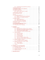
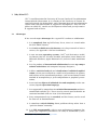
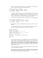
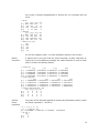
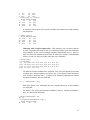
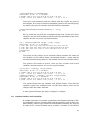
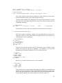
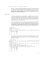
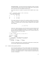
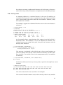
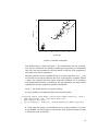
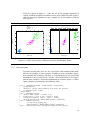
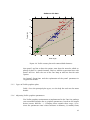
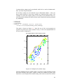
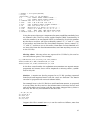
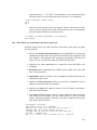
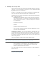
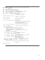
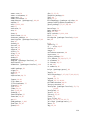
Actual vs. modelled straw yields
●
●●
●
●
●
●
●
●
●
●
●
● ●●
●
●
●
5.0
●
●
●
●
●
●
●
●
●
●
● ●
●
●
●
●
●●
●
●
●● ● ●
●
●
●
● ●● ●● ● ●●●
●●
● ●
●
●
●
●● ●● ● ●●
● ● ●
●
● ●
●
● ●
●
●
●
●
●
●●●
●● ● ●●
●
●●●●● ● ● ●● ● ● ●
● ●
●
●
●
●●● ●
●
● ● ●
●●●●
●
●●
●
●●
●●
●
● ●● ● ●
● ● ●● ●
●
●
●
● ● ●● ●
●
●
●
●
●
●● ● ●
●● ●● ●●
● ●●●
● ●●
● ●●
●●
●
●
● ●●
●●● ● ●
●● ●
● ●●
●
●
●
●
●
● ● ●●●
●●
● ● ●
● ● ●
●
●● ●
● ● ● ●●
●
●
●
●
●●
● ●
●●
●● ●
●
●●●
● ●
●
● ●● ●
●
●●●●●
●●
●●●●
●
●
● ●● ●
●●
●● ●● ●
●
●
● ● ●● ●● ●●●● ●
●● ● ●●●●
● ●●●
●
● ●
●
●
●●
●●
●● ● ●
●
●●
● ● ●●
●
●●●
●
●
●● ● ●
●
●
●
●
●
●● ●
● ● ●●
● ● ●
●● ●
● ●●●
● ●●●
●● ● ●● ●●●
●
●
●
●
●
●
●
●
●
●
●
● ●● ● ● ●
●●●●●
●
●
● ●●
●
●●
●
●● ●
●●
●● ●
● ●
● ●●●
● ● ● ● ●● ●●● ●
● ●●
● ●
●●
●●●
●●
● ●
●● ● ●●●●
●
● ●
●
●
●
●●
●
●● ● ●
●
●
●● ●
●
●
●
●●
●● ● ● ● ●●
8
●
●
●
4.5
●
4.0
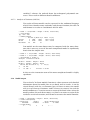
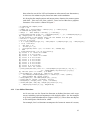
Grain yield, lbs per plot
●
●
●
3.5
7
Actual
6
5
●
●
●
●
●
●
● ●
●
●
●
●
3.0
●
●
●
●
●
4
●
4
5
6
7
8
9
1
3
5
7
Modelled
9
11
13
15
17
19
21
23
25
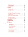
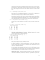
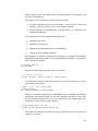
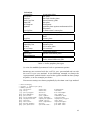
Column number
60
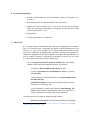
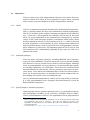
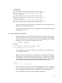
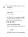
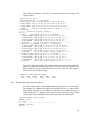
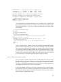
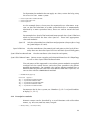
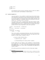
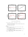
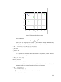
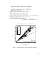
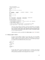
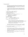
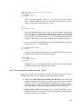
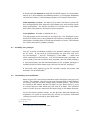
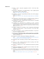
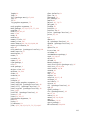
Frequency histogram, Meuse lead concentration
53
335000
330000
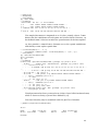
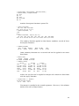
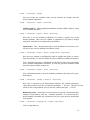
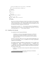
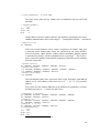
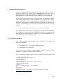
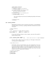
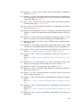
N
17 17
4
1
3
3
320000
10
12
0
100
200
300
400
325000
17
1
0
0
1
500
600
315000
30
20
26
0
Frequency
40
340000
50
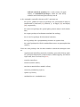
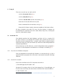
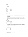
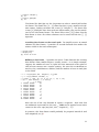
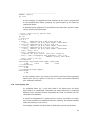
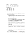
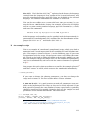
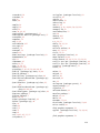
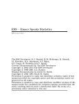
GLS 2nd−order trend surface, subsoil clay %
700
lead concentration, mg kg−1
Counts shown above bar, actual values shown with rug plot
660000
670000
680000
E
690000
700000
Contents
0 If you are impatient . . .
1
1 What is R?
1
2 Why R for ITC?
2.1 Advantages . . . . . . . . . . . . . . . . . . . .
2.2 Disadvantages . . . . . . . . . . . . . . . . . .
2.3 Alternatives . . . . . . . . . . . . . . . . . . . .
2.3.1 S-PLUS . . . . . . . . . . . . . . . . . . .
2.3.2 Statistical packages . . . . . . . . . . .
2.3.3 Special-purpose statistical programs
2.3.4 Spreadsheets . . . . . . . . . . . . . . .
2.3.5 Applied mathematics programs . . .
.
.
.
.
.
.
.
.
3
3
4
5
5
5
5
6
6
.
.
.
.
.
.
.
.
.
.
.
.
.
.
.
.
7
7
7
7
8
8
9
9
10
10
11
13
14
14
16
17
18
.
.
.
.
.
.
.
.
.
19
19
20
21
22
24
25
30
34
36
3 Using R
3.1 R console GUI . . . . . . . . . . . . . . . . . .
3.1.1 On your own Windows computer .
3.1.2 On the ITC network . . . . . . . . . .
3.1.3 Running the R console GUI . . . . .
3.1.4 Setting up a workspace in Windows
3.1.5 Saving your analysis steps . . . . . .
3.1.6 Saving your graphs . . . . . . . . . .
3.2 Working with the R command line . . . . .
3.2.1 The command prompt . . . . . . . .
3.2.2 On-line help in R . . . . . . . . . . . .
3.3 The RStudio development environment .
3.4 The Tinn-R code editor . . . . . . . . . . .
3.5 Writing and running scripts . . . . . . . . .
3.6 The Rcmdr GUI . . . . . . . . . . . . . . . . .
3.7 Loading optional packages . . . . . . . . . .
3.8 Sample datasets . . . . . . . . . . . . . . . .
4 The
4.1
4.2
4.3
4.4
4.5
4.6
4.7
4.8
4.9
.
.
.
.
.
.
.
.
.
.
.
.
.
.
.
.
.
.
.
.
.
.
.
.
.
.
.
.
.
.
.
.
.
.
.
.
.
.
.
.
.
.
.
.
.
.
.
.
.
.
.
.
.
.
.
.
.
.
.
.
.
.
.
.
.
.
.
.
.
.
.
.
.
.
.
.
.
.
.
.
.
.
.
.
.
.
.
.
.
.
.
.
.
.
.
.
.
.
.
.
.
.
.
.
.
.
.
.
.
.
.
.
.
.
.
.
.
.
.
.
.
.
.
.
.
.
.
.
.
.
.
.
.
.
.
.
.
.
.
.
.
.
.
.
.
.
.
.
.
.
.
.
.
.
.
.
.
.
.
.
.
.
.
.
.
.
.
.
.
.
.
.
.
.
.
.
.
.
.
.
.
.
.
.
S language
Command-line calculator and mathematical operators
Creating new objects: the assignment operator . . . . .
Methods and their arguments . . . . . . . . . . . . . . . .
Vectorized operations and re-cycling . . . . . . . . . . .
Vector and list data structures . . . . . . . . . . . . . . .
Arrays and matrices . . . . . . . . . . . . . . . . . . . . . .
Data frames . . . . . . . . . . . . . . . . . . . . . . . . . . .
Factors . . . . . . . . . . . . . . . . . . . . . . . . . . . . . .
Selecting subsets . . . . . . . . . . . . . . . . . . . . . . . .
.
.
.
.
.
.
.
.
.
.
.
.
.
.
.
.
.
.
.
.
.
.
.
.
.
.
.
.
.
.
.
.
.
.
.
.
.
.
.
.
.
.
.
.
.
.
.
.
.
.
.
.
.
.
.
.
.
.
.
.
.
.
.
.
.
.
.
.
.
.
.
.
.
.
.
.
.
.
.
.
.
.
.
.
.
.
.
.
.
.
.
.
.
.
.
.
.
.
.
Version 4.0 Copyright © D G Rossiter 2003 – 2012. All rights reserved.
Non-commercial reproduction and dissemination of the work as a whole
freely permitted if this original copyright notice is included. To adapt or
translate please contact the author.
ii
4.9.1 Simultaneous operations on subsets
4.10 Rearranging data . . . . . . . . . . . . . . . . .
4.11 Random numbers and simulation . . . . . .
4.12 Character strings . . . . . . . . . . . . . . . . .
4.13 Objects and classes . . . . . . . . . . . . . . .
4.13.1 The S3 and S4 class systems . . . . .
4.14 Descriptive statistics . . . . . . . . . . . . . .
4.15 Classification tables . . . . . . . . . . . . . . .
4.16 Sets . . . . . . . . . . . . . . . . . . . . . . . . .
4.17 Statistical models in S . . . . . . . . . . . . . .
4.17.1 Models with categorical predictors .
4.17.2 Analysis of Variance (ANOVA) . . . .
4.18 Model output . . . . . . . . . . . . . . . . . . .
4.18.1 Model diagnostics . . . . . . . . . . . .
4.18.2 Model-based prediction . . . . . . . .
4.19 Advanced statistical modelling . . . . . . . .
4.20 Missing values . . . . . . . . . . . . . . . . . .
4.21 Control structures and looping . . . . . . . .
4.22 User-defined functions . . . . . . . . . . . . .
4.23 Computing on the language . . . . . . . . . .
.
.
.
.
.
.
.
.
.
.
.
.
.
.
.
.
.
.
.
.
.
.
.
.
.
.
.
.
.
.
.
.
.
.
.
.
.
.
.
.
.
.
.
.
.
.
.
.
.
.
.
.
.
.
.
.
.
.
.
.
.
.
.
.
.
.
.
.
.
.
.
.
.
.
.
.
.
.
.
.
.
.
.
.
.
.
.
.
.
.
.
.
.
.
.
.
.
.
.
.
.
.
.
.
.
.
.
.
.
.
.
.
.
.
.
.
.
.
.
.
.
.
.
.
.
.
.
.
.
.
.
.
.
.
.
.
.
.
.
.
.
.
.
.
.
.
.
.
.
.
.
.
.
.
.
.
.
.
.
.
.
.
.
.
.
.
.
.
.
.
.
.
.
.
.
.
.
.
.
.
39
40
41
43
44
45
48
50
51
52
55
57
57
59
61
62
63
64
65
67
5 R graphics
5.1 Base graphics . . . . . . . . . . . . . . . . . . . . . .
5.1.1 Mathematical notation in base graphics .
5.1.2 Returning results from graphics methods
5.1.3 Types of base graphics plots . . . . . . . .
5.1.4 Interacting with base graphics plots . . . .
5.2 Trellis graphics . . . . . . . . . . . . . . . . . . . . .
5.2.1 Univariate plots . . . . . . . . . . . . . . . .
5.2.2 Bivariate plots . . . . . . . . . . . . . . . . .
5.2.3 Triivariate plots . . . . . . . . . . . . . . . .
5.2.4 Panel functions . . . . . . . . . . . . . . . . .
5.2.5 Types of Trellis graphics plots . . . . . . .
5.2.6 Adjusting Trellis graphics parameters . .
5.3 Multiple graphics windows . . . . . . . . . . . . . .
5.3.1 Switching between windows . . . . . . . . .
5.4 Multiple graphs in the same window . . . . . . .
5.4.1 Base graphics . . . . . . . . . . . . . . . . . .
5.4.2 Trellis graphics . . . . . . . . . . . . . . . . .
5.5 Colours . . . . . . . . . . . . . . . . . . . . . . . . . .
.
.
.
.
.
.
.
.
.
.
.
.
.
.
.
.
.
.
.
.
.
.
.
.
.
.
.
.
.
.
.
.
.
.
.
.
.
.
.
.
.
.
.
.
.
.
.
.
.
.
.
.
.
.
.
.
.
.
.
.
.
.
.
.
.
.
.
.
.
.
.
.
.
.
.
.
.
.
.
.
.
.
.
.
.
.
.
.
.
.
.
.
.
.
.
.
.
.
.
.
.
.
.
.
.
.
.
.
.
.
.
.
.
.
.
.
.
.
.
.
.
.
.
.
.
.
.
.
.
.
.
.
.
.
.
.
.
.
.
.
.
.
.
.
69
69
73
75
75
77
77
77
78
79
81
82
82
84
85
85
85
86
86
6 Preparing your own data for R
6.1 Preparing data directly in R . .
6.2 A GUI data editor . . . . . . . .
6.3 Importing data from a CSV file
6.4 Importing images . . . . . . . .
.
.
.
.
.
.
.
.
.
.
.
.
.
.
.
.
.
.
.
.
.
.
.
.
.
.
.
.
.
.
.
.
91
91
92
93
96
7 Exporting from R
.
.
.
.
.
.
.
.
.
.
.
.
.
.
.
.
.
.
.
.
.
.
.
.
.
.
.
.
.
.
.
.
.
.
.
.
.
.
.
.
.
.
.
.
.
.
.
.
.
.
.
.
.
.
.
.
.
.
.
.
.
.
.
.
.
.
.
.
.
.
.
.
.
.
.
.
.
.
.
.
.
.
.
.
99
iii
8 Reproducible data analysis
8.1 The NoWeb document
8.2 The LATEX document . .
8.3 The PDF document . .
8.4 Graphics in Sweave . .
.
.
.
.
.
.
.
.
.
.
.
.
.
.
.
.
.
.
.
.
.
.
.
.
.
.
.
.
.
.
.
.
.
.
.
.
.
.
.
.
.
.
.
.
.
.
.
.
.
.
.
.
.
.
.
.
.
.
.
.
.
.
.
.
.
.
.
.
101
101
102
103
104
9 Learning R
9.1 Task views . . . . . . . . . . . . . . . .
9.2 R tutorials and introductions . . . .
9.3 Textbooks using R . . . . . . . . . . .
9.4 Technical notes using R . . . . . . .
9.5 Web Pages to learn R . . . . . . . . .
9.6 Keeping up with developments in R
.
.
.
.
.
.
.
.
.
.
.
.
.
.
.
.
.
.
.
.
.
.
.
.
.
.
.
.
.
.
.
.
.
.
.
.
.
.
.
.
.
.
.
.
.
.
.
.
.
.
.
.
.
.
.
.
.
.
.
.
.
.
.
.
.
.
.
.
.
.
.
.
.
.
.
.
.
.
.
.
.
.
.
.
.
.
.
.
.
.
.
.
.
.
.
.
105
105
105
106
107
107
108
.
.
.
.
.
.
110
110
112
113
115
116
117
A Obtaining your own copy of R
A.1 Installing new packages . . . . . . . . . . . . . . . . . . . . . . .
A.2 Customizing your installation . . . . . . . . . . . . . . . . . . . .
A.3 R in different human languages . . . . . . . . . . . . . . . . . . .
119
121
121
122
B An example script
123
C An example function
126
References
128
Index of R concepts
133
.
.
.
.
.
.
.
.
.
.
.
.
.
.
.
.
.
.
.
.
.
.
.
.
.
.
.
.
10 Frequently-asked questions
10.1 Help! I got an error, what did I do wrong? . . . .
10.2 Why didn’t my command(s) do what I expected?
10.3 How do I find the method to do what I want? . .
10.4 Memory problems . . . . . . . . . . . . . . . . . . .
10.5 What version of R am I running? . . . . . . . . . .
10.6 What statistical procedure should I use? . . . . .
.
.
.
.
.
.
.
.
.
.
.
.
.
.
.
.
.
.
.
.
.
.
.
.
.
.
.
.
.
.
.
.
.
.
.
.
.
.
.
.
.
.
List of Figures
1
2
3
4
5
6
7
8
9
10
11
12
13
14
The RStudio screen . . . . . . . . . . . . . . . . . . . . . .
The Tinn-R screen . . . . . . . . . . . . . . . . . . . . . . .
The R Commander screen . . . . . . . . . . . . . . . . . .
Regression diagnostic plots . . . . . . . . . . . . . . . . .
Finding the closest point . . . . . . . . . . . . . . . . . . .
Default scatterplot . . . . . . . . . . . . . . . . . . . . . . .
Plotting symbols . . . . . . . . . . . . . . . . . . . . . . . .
Custom scatterplot . . . . . . . . . . . . . . . . . . . . . .
Scatterplot with math symbols, legend and model lines
Some interesting base graphics plots . . . . . . . . . . .
Trellis density plots . . . . . . . . . . . . . . . . . . . . . .
Trellis scatter plots . . . . . . . . . . . . . . . . . . . . . .
Trellis trivariate plots . . . . . . . . . . . . . . . . . . . . .
Trellis scatter plot with some added elements . . . . .
.
.
.
.
.
.
.
.
.
.
.
.
.
.
.
.
.
.
.
.
.
.
.
.
.
.
.
.
.
.
.
.
.
.
.
.
.
.
.
.
.
.
.
.
.
.
.
.
.
.
.
.
.
.
.
.
13
14
16
60
66
70
71
73
74
76
78
79
80
82
iv
15
16
17
18
19
20
21
Available colours . . . . . . . . . . . . . . . . . . . . . .
Example of a colour ramp . . . . . . . . . . . . . . . .
R graphical data editor . . . . . . . . . . . . . . . . . .
Example PDF produced by Sweave and LATEX . . . . .
Results of an RSeek search . . . . . . . . . . . . . . . .
Results of an R site search . . . . . . . . . . . . . . . .
Visualising the variability of small random samples
.
.
.
.
.
.
.
.
.
.
.
.
.
.
.
.
.
.
.
.
.
.
.
.
.
.
.
.
.
.
.
.
.
.
.
.
.
.
.
.
.
.
87
89
93
103
108
109
125
1
2
3
4
Methods for adding to an existing base graphics plot
Base graphics plot types . . . . . . . . . . . . . . . . . .
Trellis graphics plot types . . . . . . . . . . . . . . . . .
Packages in the base R distribution for Windows . . .
.
.
.
.
.
.
.
.
.
.
.
.
.
.
.
.
. 71
. 75
. 83
. 120
List of Tables
v
0
If you are impatient . . .
1. Install R and RStudio on your MS-Windows, Mac OS/X or Linux system (§A);
2. Run RStudio; this will automatically start R within it;
3. Follow one of the tutorials (§9.2) such as my “Using the R Environment for Statistical Computing: An example with the Mercer & Hall
wheat yield dataset”1 [48];
4. Experiment!
5. Use this document as a reference.
1
What is R?
R is an open-source environment for statistical computing and visualisation. It is based on the S language developed at Bell Laboratories in the
1980’s [20], and is the product of an active movement among statisticians for a powerful, programmable, portable, and open computing environment, applicable to the most complex and sophsticated problems, as
well as “routine” analysis, without any restrictions on access or use. Here
is a description from the R Project home page:2
“R is an integrated suite of software facilities for data manipulation, calculation and graphical display. It includes:
• an effective data handling and storage facility,
• a suite of operators for calculations on arrays, in particular matrices,
• a large, coherent, integrated collection of intermediate tools
for data analysis,
• graphical facilities for data analysis and display either onscreen or on hardcopy, and
• a well-developed, simple and effective programming language which includes conditionals, loops, user-defined recursive functions and input and output facilities.”
The last point has resulted in another major feature:
• Practising statisticians have implemented hundreds of spe1
2
http://www.itc.nl/personal/rossiter/pubs/list.html#pubs_m_R, item 2
http://www.r-project.org/
1
cialised statistical produres for a wide variety of applications as contributed packages, which are also freelyavailable and which integrate directly into R.
A few examples especially relevant to ITC’s mission are:
• the gstat, geoR and spatial packages for geostatistical analysis,
contributed by Pebesma [33], Ribeiro, Jr. & Diggle [39] and Ripley
[40], respectively;
• the spatstat package for spatial point-pattern analysis and simulation;
• the vegan package of ordination methods for ecology;
• the circular package for directional statistics;
• the sp package for a programming interface to spatial data;
• the rgdal package for GDAL-standard data access to geographic data
sources;
There are also packages for the most modern statistical techniques such
as:
• sophisticated modelling methods, including generalized linear models, principal components, factor analysis, bootstrapping, and robust
regression; these are listed in §4.19;
• wavelets (wavelet);
• neural networks (nnet);
• non-linear mixed-effects models (nlme);
• recursive partitioning (rpart);
• splines (splines);
• random forests (randomForest)
2
2
Why R for ITC?
“ITC” is an abbreviation for University of Twente, Faculty of Geo-information
Science& Earth Observation. It is a faculty of the University of Twente located in Enschede, the Netherlands, with a thematic focus on geo-information
science and earth observation in support of development. Thus the two
pillars on which ITC stands are development-related and geo-information.
R supports both of these.
2.1
Advantages
R has several major advantages for a typical ITC student or collaborator:
1. It is completely free and will always be so, since it is issued under
the GNU Public License;3
2. It is freely-available over the internet, via a large network of mirror
servers; see Appendix A for how to obtain R;
3. It runs on many operating systems: Unix© and derivatives including Darwin, Mac OS X, Linux, FreeBSD, and Solaris; most flavours of
Microsoft Windows; Apple Macintosh OS; and even some mainframe
OS.
4. It is the product of international collaboration between top computational statisticians and computer language designers;
5. It allows statistical analysis and visualisation of unlimited sophistication; you are not restricted to a small set of procedures or options,
and because of the contributed packages, you are not limited to one
method of accomplishing a given computation or graphical presentation;
6. It can work on objects of unlimited size and complexity with a consistent, logical expression language;
7. It is supported by comprehensive technical documentation and usercontributed tutorials (§9). There are also several good textbooks on
statistical methods that use R (or S) for illustration.
8. Every computational step is recorded, and this history can be saved
for later use or documentation.
9. It stimulates critical thinking about problem-solving rather than a
“push the button” mentality.
10. It is fully programmable, with its own sophisticated computer language (§4). Repetitive procedures can easily be automated by user3
http://www.gnu.org/copyleft/gpl.html
3
written scripts (§3.5). It is easy to write your own functions (§B),
and not too difficult to write whole packages if you invent some new
analysis;
11. All source code is published, so you can see the exact algorithms being used; also, expert statisticians can make sure the code is correct;
12. It can exchange data in MS-Excel, text, fixed and delineated formats
(e.g. CSV), so that existing datasets are easily imported (§6), and results computed in R are easily exported (§7).
13. Most programs written for the commercial S-PLUS program will run
unchanged, or with minor changes, in R (§2.3.1).
2.2
Disadvantages
R has its disadvantages (although “every disadvantage has its advantage”):
1. The default Windows and Mac OS X graphical user interface (GUI)
(§3.1) is limited to simple system interaction and does not include
statistical procedures. The user must type commands to enter data,
do analyses, and plot graphs. This has the advantage that the user
has complete control over the system. The Rcmdr add-on package
(§3.6) provides a reasonable GUI for common tasks, and there are
various development environments for R, such as RStudio (§3.3).
2. The user must decide on the analysis sequence and execute it stepby-step. However, it is easy to create scripts with all the steps in
an analysis, and run the script from the command line or menus
(§3.5); scripts can be preared in code editors built into GUI versions
of R or separate front-ends such as Tinn-R (§3.5) or RStudio (§3.3). A
major advantage of this approach is that intermediate results can be
reviewed, and scripts can be edited and run as batch processes.
3. The user must learn a new way of thinking about data, as data
frames (§4.7) and objects each with its class, which in turn supports
a set of methods (§4.13). This has the advantage common to objectoriented languages that you can only operate on an object according
to methods that make sense4 and methods can adapt to the type of
object.5
4. The user must learn the S language (§4), both for commands and
the notation used to specify statistical models (§4.17). The S statistical modelling language is a lingua franca among statisticians, and
provides a compact way to express models.
4
5
For example, the t (transpose) method only can be applied to matrices
For example, the summary and plot methods give different results depending on the
class of object.
4
2.3
Alternatives
There are many ways to do computational statistics; this section discusses
them in relation to R. None of these programs are open-source, meaning
that you must trust the company to do the computations correctly.
2.3.1
S-PLUS
S-PLUS is a commercial program distributed by the Insightful corporation,6
and is a popular choice for large-scale commerical statistical computing.
Like R, it is a dialect of the original S language developed at Bell Laboratories.7 S-PLUS has a full graphical user interface (GUI); it may be also used
like R, by typing commands at the command line interface or by running
scripts. It has a rich interactive graphics environment called Trellis, which
has been emulated with the lattice package in R (§5.2). S-PLUS is licensed
by local distributors in each country at prices ranging from moderate to
high, depending factors such as type of licensee and application, and how
many computers it will run on. The important point for ITC R users is that
their expertise will be immediately applicable if they later use S-PLUS in a
commercial setting.
2.3.2
Statistical packages
There are many statistical packages, including MINITAB, SPSS, Statistica,
Systat, GenStat, and BMDP,8 which are attractive if you are already familiar
with them or if you are required to use them at your workplace. Although
these are programmable to varying degrees, it is not intended that specialists develop completely new algorithms. These must be purchased from
local distributors in each country, and the purchaser must agree to the license terms. These often have common analyses built-in as menu choices;
these can be convenient but it is tempting to use them without fully understanding what choices they are making for you.
SAS is a commercial competitor to S-PLUS, and is used widely in industry.
It is fully programmable with a language descended from PL/I (used on
IBM mainframe computers).
2.3.3
Special-purpose statistical programs
Some programs adress specific statistical issues, e.g. geostatistical analysis
and interpolation (SURFER, gslib, GEO-EAS), ecological analysis (FRAGSTATS), and ordination (CONOCO). The algorithms in these programs have
6
http://www.insightful.com/
There are differences in the language definitions of S, R, and S-PLUS that are important
to programmers, but rarely to end-users. There are also differences in how some
algorithms are implemented, so the numerical results of an identical method may be
somewhat different.
8
See the list at http://www.stata.com/links/stat_software.html
7
5
or can be programmed as an R package; examples are the gstat program
for geostatistical analysis9 [35], which is now available within R [33], and
the vegan package for ecological statistics.
2.3.4
Spreadsheets
Microsoft Excel is useful for data manipulation. It can also calculate some
statistics (means, variances, . . . ) directly in the spreadsheet. This is also
an add-on module (menu item Tools | Data Analysis. . . ) for some common
statistical procedures including random number generation. Be aware that
Excel was not designed by statisticians. There are also some commercial add-on packages for Excel that provide more sophisticated statistical
analyses. Excel’s default graphics are easy to produce, and they may be
customized via dialog boxes, but their design has been widely criticized.
Least-squares fits on scatterplots give no regression diagnostics, so this is
not a serious linear modelling tool.
OpenOffice10 includes an open-source and free spreadsheet (Open Office
Calc) which can replace Excel.
2.3.5
Applied mathematics programs
MATLAB is a widely-used applied mathematics program, especially suited
to matrix maniupulation (as is R, see §4.6), which lends itself naturally
to programming statistical algorithms. Add-on packages are available for
many kinds of statistical computation. Statistical methods are also programmable in Mathematica.
9
10
http://www.gstat.org/
http://www.openoffice.org/
6
3
Using R
There are several ways to work with R:
• with the R console GUI (§3.1);
• with the RStudio IDE (§3.3);
• with the Tinn-R editor and the R console (§3.4);
• from one of the other IDE such as JGR;
• from a command line R interface (CLI) (§3.2);
• from the ESS (Emacs Speaks Statistics) module of the Emacs editor.
Of these, RStudio is for most ITC users the best choice; it contains an
R command line interface but with a code editor, help text, a workspace
browser, and graphic output.
3.1
R console GUI
The default interface for both Windows and Mac OS/X is a simple GUI.
We refer to these as “R console GUI” because they provide an easy-to-use
interface to the R command line, a simple script editor, graphics output,
and on-line help; they do not contain any menus for data manipulation or
statistical procedures.
R for Linux has no GUI; however, several independent Linux programs11
provide a GUI development environment; an example is RStudio (§3.3).
3.1.1
On your own Windows computer
You can download and install R for Windows as instructed in §A, as for a
typical Windows program; this will create a Start menu item and a desktop
shortcut.
3.1.2
On the ITC network
R has been installed on the ITC corporate network at:
\\Itcnt03\Apps\R\bin\RGui.exe
For most ITC accounts drive P: has been mapped to \\Itcnt03\Apps, so
R can be accessed using this drive letter instead of the network address:
P:\R\bin\RGui.exe
11
http://www.linuxlinks.com/article/20110306113701179/GUIsforR.html
7
You can copy this to your local desktop as a shortcut.
Documentation has been installed at:
P:\R\doc
3.1.3
Running the R console GUI
R GUI for Windows is started like any Windows program: from the Start
menu, from a desktop shortcut, or from the application’s icon in Explorer.
By default, R starts in the directory where it was installed, which is not
where you should store your projects. If you are using the copy of R on
the ITC network, you do not have write permission to this directory, so you
won’t be able to save any data or session information there. So, you will
probably want to change your workspace, as explained in §3.1.4. You can
also create a desktop shortcut or Start menu item for R, also as explained
in §3.1.4.
To stop an R session, type q() at the command prompt12 , or select the
File | Exit menu item in the Windows GUI.
3.1.4
Setting up a workspace in Windows
An important concept in R is the workspace, which contains the local
data and procedures for a given statistics project. Under Windows this is
usually determined by the folder from which R is started.
Under Windows, the easiest way to set up a statistics project is:
1. Create a shortcut to RGui.exe on your desktop;
2. Modify its properties so that its in your working directory rather
than the default (e.g. P:\R\bin).
Now when you double-click on the shortcut, it will start R in the directory
of your choice. So, you can set up a different shortcut for each of your
projects.
Another way to set up a new statistics project in R is:
1. Start R as just described: double-click the icon for program RGui.exe
in the Explorer;
2. Select the File | Change Directory ... menu item in R;
3. Select the directory where you want to work;
12
This is a special case of the q method
8
4. Exit R by selecting the File | Exit menu item in R, or typing the
q() command; R will ask “Save workspace image?”; Answer y (Yes).
This will create two files in your working directory: .Rhistory and
.RData.
The next time you want to work on the same project:
1. Open Explorer and navigate to the working directory
2. Double-click on the icon for file .RData
R should open in that directory, with your previous workspace already
loaded. (If R does not open, instead Explorer will ask you what programs
should open files of type .RData; navigate to the program RGui.exe and
select it.)
If you don’t see the file .RData in your Explorer, this is because Windows
Revealing hid- considers any file name that begins with “.” to be a ‘hidden’ file. You need
den files in to select the Tools | Folder options in Explorer, then the View tab,
Windows
and click the radio button for Show hidden files and folders. You
must also un-check the box for Hide file extensions for known file
types.
3.1.5
Saving your analysis steps
The File | Save to file ... menu command will save the entire console contents, i.e. both your commands and R’s response, to a text file,
which you can later review and edit with any text editor. This is useful for
cutting-and-pasting into your reports or thesis, and also for writing scripts
to repeat procedures.
3.1.6
Saving your graphs
In the Windows version of R, you can save any graphical output for insertion into documents or printing. If necessary, bring the graphics window to the front (e.g. click on its title bar), select menu command File |
Save as ..., and then one of the formats. Most useful for insertion into
MS-Word documents is Metafile; most useful for LATEX is Postscript; most
useful for PDFLaTeX and stand-alone printing is PDF. You can later review
your saved graphics with programs such as Windows Picture Editor. If you
want to add other graphical elements, you may want to save as a PNG or
JPEG; however in most cases it is cleaner to add annotations within R itself.
You can also review graphics within the Windows R GUI itself. Create the
first graph, bring the graphics window to foreground, and then select the
menu command History | Recording. After this all graphs are automatically saved within R, and you can move through them with the up and
down arrow keys.
9
You can also write your graphics commands directly to a graphics file in
many formats, e.g. PDF or JPEG. You do this by opening a graphics device,
writing the commands, and then closing the device. You can get a list of
graphics devices (formats) available on your system with ?Devices (note
the upper-case D).
For example, to write a PDF file, we open a PDF graphics device with the
pdf function, write to it, and then close it with the dev.off function:
pdf("figure1.pdf", h=6, w=6)
hist(rnorm(100), main="100 random values from N[0,1])")
dev.off()
Note the use of the optional height= and width= arguments (here abbreviated h= and w=) to specifiy the size of the PDF file (in US inches); this
affects the font sizes. The defaults are both 7 inches (17.18 cm).
3.2
Working with the R command line
These instructions apply to the simple R GUI and the R command line
interface window within RStudio. One of the windows in these interfaces
is the command line, also called the R console.
It is possible to work directly with the command line and no GUI:
• Under Linux and Mac OS/X, at the shell prompt just type R; there are
various startup options which you can see with R -help.
• Under Windows
3.2.1
The command prompt
You perform most actions in R by typing commands in a command line
interface window,13 in response to a command prompt, which usually
looks like this:
>
The > is a prompt symbol displayed by R, not typed by you. This is R’s
way of telling you it’s ready for you to type a command.
Type your command and press the Enter or Return keys; R will execute
your command.
If your entry is not a complete R command, R will prompt you to complete
it with the continuation prompt symbol:
13
An alternative for some analyses is the Rcmdr GUI explained in §3.6.
10
+
R will accept the command once it is syntactically complete; in particular
the parentheses must balance. Once the command is complete, R then
presents its results in the same command line interface window, directly
under your command.
If you want to abort the current command (i.e. not complete it), press the
Esc (“escape”) key.
For example, to draw 500 samples from a binomial distribution of 20 trials
with a 40% chance of success14 you would first use the rbinom method and
then summarize it with the summary method, as follows:15
> x <- rbinom(500,20,.4)
> summary(x)
Min. 1st Qu. Median
2.000
7.000
8.000
Mean 3rd Qu.
8.232 10.000
Max.
15.000
This could also have been entered on several lines:
> x <- rbinom(
+ 500,20,.4
+ )
You can use any white space to increase legibility, except that the assignment symbol <- must be written together:
> x
<-
rbinom(500,
20,
0.4)
R is case-sensitive; that is, method rbinom must be written just that way,
not as Rbinom or RBINOM (these might be different methods). Variables are
also case-sensitive: x and X are different names.
Some methods produce output in a separate graphics window:
> hist(x)
3.2.2
On-line help in R
Both the base R system and contributed packages have extensive help
within the running R environment.
Individual
methods
In Windows , you can use the Help menu and navigate to the method you
want to understand. You can also get help on any method with the ?
14
This simulates, for example, the number of women who would be expected, by chance,
to present their work at a conference where 20 papers are to be presented, if the
women make up 40% of the possible presenters.
15
Your output will probably be somewhat different; why?
11
method, typed at the command prompt; this is just a shorthand for the
help method:
For example, if you don’t know the format of the rbinom method used
above. Either of these two forms:
> ?rbinom
> help(rbinom)
will display a text page with the syntax and options for this method. There
are examples at the end of many help topics, with executable code that you
can experiment with to see just how the method works.
Searching for
methods
If you don’t know the method name, you can search the help for relevant
methods using the help.search method16 :
> help.search("binomial")
will show a window with all the methods that include this word in their description, along with the packages where these methods are found, whether
already loaded or not.
In the list shown as a result of the above method, we see the Binomial
(stats) topic; we can get more information on it with the ? method; this
is written as the ? character immediately followed by the method name:
> ?Binomial
This shows the named topic, which explains the rbinom (among other)
methods.
Vignettes
Packages have a long list of methods, each of which has its own documentation as explained above. Some packages are documented as a whole by
so-called vignettes17 ; for now most packages do not have one, but more
will be added over time.
You can see a list of the vignettes installed on your system with the vignette
method with an empty argument:
> vignette()
and then view a specific vignette by naming it:
> vignette("sp")
16
17
also available via the Help | Search help ... menu item
from the OED meaning “a brief verbal description of a person, place, etc.; a short
descriptive or evocative episode in a play, etc.”
12
3.3
The RStudio development environment
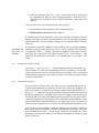
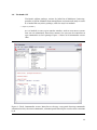
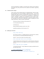
RStudio18 is an excellent cross-platform19 integrated development environment for R. A screenshot is shown in Figure 1. This environment includes the command line interface, a code editor, output graphs, history,
help, workspace contents, and package manager all in one atttractive interface. The typical use is: (1) open a script or start a new script; (2) change
the working directory to this script’s location; (3) write R code in the script;
(4) pass lines of code from the script to the command line interface and
evaluate the output; (5) examine any graphs and save for later use.
Figure 1: The RStudio screen
18
19
http://www.rstudio.org/
Windows, Mac OS/X, Linux
13
3.4
The Tinn-R code editor
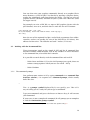
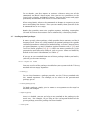
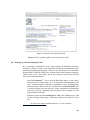
For Windows user, the Tinn-R code editor for Windows20 is recommended
for those who do not choose to use RStudio. This is tightly integrated with
the Windows R GUI, as shown in Figure 2. R code is syntax-highlighted and
there is extensive help within the editor to select the proper commands
and arguments. Commands can be sent directly from the editor to R, or
saved in a file and sourced.
Figure 2: The Tinn-R screen, with the R command line interface also visible
3.5
Writing and running scripts
After you have worked out an analysis by typing a sequence of commands,
you will probably want to re-run them on edited data, new data, subsets
etc. This is easy to do by means of scripts, which are simply lists of commands in a file, written exactly as you would type them at the command
20
http://www.sciviews.org/Tinn-R/
14
line interface. They are run with the source method. A useful feature
of scripts is that you can include comments (lines that begin with the #
character) to explain to yourself or others what the script is doing and
why.
Here’s a step-by-step description of how to create and run a simple script
which draws two random samples from a normal distribution and computes their correlation:21
1. Open a new document in a plain-text editor, i.e., one that does not
insert any formatting. Under MS-Windows you can use Notepad or
Wordpad; if you are using Tinn-R or RStudio open a new script.
2. Type in the following lines:
x <- rnorm(100, 180, 20)
y <- rnorm(100, 180, 20)
plot(x, y)
cor.test(x, y)
3. Save the file with the name test.R, in a convenient directory.
4. Start R (if it’s not already running)
5. In R, select menu command File | Source R code ...
6. In the file selection dialog, locate the file test.R that you just saved
(changing directories if necessary) and select it; R will run the script.
7. Examine the output.
You can source the file directly from the command line. Instead of steps
5 and 6 above, just type source("test.R") at the R command prompt
(assuming you’ve switched to the directory where you saved the script).
Appendix B contains an example of a more sophisticated script.
For serious work with R you should use a more powerful text editor. The
R for Windows, R for Mac OS X and JGR interfaces include built-in editors; another choice on Windows is WinEdt22 . And both RStudio (§3.3)
and Tinn_R (§3.4) have code editors. For the ultimate in flexibility and
power, try emacs23 with the ESS (Emacs Speaks Statistics) module24 ; learning emacs is not trivial but rather an investment in a lifetime of efficient
computing.
21
What is the expected value of this correlation cofficient?
http://www.winedt.com/
23
http://en.wikipedia.org/wiki/Emacs
24
http://stat.ethz.ch/ESS/
22
15
3.6
The Rcmdr GUI
The Rcmdr add-on package, written by John Fox of McMaster University,
provides a GUI for common data management and statistical analysis tasks.
It is loaded like any other package, with the require method:
> require("Rcmdr")
As it is loaded, it starts up in another window, with its own menu system.
You can run commands from these menus, but you can also continue to
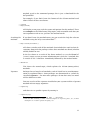
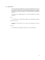
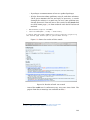
type commands at the R prompt. Figure 3 shows an R Commander screen
shot.
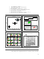
Figure 3: The R Commander screen: Menu bar at the top; a top panel showing commands
submitted to R by the menu commands; a bottom panel showing the results after execution
by R
16
To use Rcmdr, you first import or activate a dataset using one of the
commands on Rcmdr’s Data menu; then you can use procedures in the
Statistics, Graphs, and Models menus. You can also create and graph
probability distributions with the Distributions menu.
When using Rcmdr, observe the commands it formats in response to your
menu and dialog box choices. Then you can modify them yourself at the
R command line or in a script.
Rcmdr also provides some nice graphics options, including scatterplots
(2D and 3D) where observations can be coloured by a classifying factor.
3.7
Loading optional packages
R starts up with a base package, which provides basic statistics and the R
language itself. There are a large number of optional packages for specific
statistical procedures which can be loaded during a session. Some of these
are quite common, e.g. MASS (“Modern Applied Statistics with S” [57]) and
lattice (Trellis graphics [50], §5.2). Others are more specialised, e.g. for
geostatistics and time-series analysis, such as gstat. Some are loaded by
default in the base R distribution (see Table 4).
If you try to run a method from one of these packages before you load it,
you will get the error message
Error: object not found
You can see a list of the packages installed on your system with the library
method with an empty argument:
> library()
To see what functions a package provides, use the library method with
the named argument. For example, to see what’s in the geostatistical
package gstat:
> library(help=gstat)
To load a package, simply give its name as an argument to the require
method, for example:
> require(gstat)
Once it is loaded, you can get help on any method in the package in the
usual way. For example, to get help on the variogram method of the
gstat package, once this package has been loaded:
> ?variogram
17
3.8
Sample datasets
R comes with many example datasets (part of the default datasets package) and most add-in packages also include example datasets. Some of
the datasets are classics in a particular application field; an example is
the iris dataset used extensively by R A Fisher to illustrate multivariate
methods.
To see the list of installed datasets, use the data method with an empty
argument:
> data()
To see the datasets in a single add-in package, use the package= argument:
> data(package="gstat")
To load one of the datasets, use its name as the argument to the data
method:
> data(iris)
The dataframe representing this dataset is now in the workspace.
18
4
The S language
R is a dialect of the S language, which has a syntax similar to ALGOL-like
programming languages such as C, Pascal, and Java. However, S is objectoriented, and makes vector and matrix operations particularly easy; these
make it a modern and attractive user and programming environment. In
this section we build up from simple to complex commands, and break
down their anatomy. A full description of the language is given in the R
Language Definition [38]25 and a comprehensive introduction is given in
the Introduction to R [36].26 This section reviews the most outstanding
features of S.
All the functions, packages and datasets mentioned in this section (as well
as the rest of this note) are indexed (§C) for quick reference.
4.1
Command-line calculator and mathematical operators
The simplest way to use R is as an interactive calculator. For example, to
compute the number of radians in one Babylonian degree of a circle:
> 2*pi/360
[1] 0.0174533
As this example shows, S has a few built-in constants, among them pi for
the mathematical constant π . The Euler constant e is not built-in, it must
be calculated with the exp function as exp(1).
If the assignment operator (explained in the next section) is not present,
the expression is evaluated and its value is displayed on the console. S has
the usual arithmetic operators +, -, *, /, ^ and some less-common ones
like %% (modulus) and %/% (integer division). Expressions are evaluated in
accordance with the usual operator precedence; parentheses may be used
to change the precedence or make it explicit:
> 3 / 2^2 + 2 * pi
[1] 7.03319
> ((3 / 2)^2 + 2) * pi
[1] 13.3518
Spaces may be used freely and do not alter the meaning of any S expression.
Common mathematical functions are provided as functions (see §4.3), including log, log10 and log2 functions to compute logarithms; exp for exponentiation; sqrt to extract square roots; abs for absolute value; round,
ceiling, floor and trunc for rounding and related operations; trigonometric functions such as sin, and inverse trigonometric functions such as
25
26
In RGui, menu command Help | Manuals | R Language Manual
In RGui, menu command Help | Manuals | R Introduction
19
asin.
> log(10); log10(10); log2(10)
[1] 2.3026
[1] 1
[1] 3.3219
> round(log(10))
[1] 2
> sqrt(5)
[1] 2.2361
sin(45 * (pi/180))
[1] 0.7071
> (asin(1)/pi)*180
[1] 90
4.2
Creating new objects: the assignment operator
New objects in the workspace are created with the assignment operator <-,
which may also be written as =:
> mu <- 180
> mu = 180
The symbol on the left side is given the value of the expression on the right
side, creating a new object (or redefining an existing one), here named
mu, in the workspace and assigning it the value of the expression, here
the scalar value 180, which is stored as a one-element vector. The twocharacter symbol <- must be written as two adjacent characters with no
spaces..
Now that mu is defined, it may be printed at the console as an expression:
> print(mu)
[1] 180
> mu
[1] 180
and it may be used in an expression:
> mu/pi
[1] 57.2958
More complex objects may be created:
> s <- seq(10)
> s
[1] 1 2 3 4
5
6
7
8
9 10
This creates a new object named s in the workspace and assigns it the vector (1 2 ...10). (The syntax of seq(10) is explained in the next section.)
Multiple assignments are allowed in the same expression:
20
> (mu <- theta <- pi/2)
[1] 1.5708
The final value of the expression, in this case the value of mu, is printed,
because the parentheses force the expression to be evaluated as a unit.
Removing objects from the workspace You can remove objects when
they are no longer needed with the rm function:
> rm(s)
> s
Error: Object "s" not found
4.3
Methods and their arguments
In the command s <- seq(10), seq is an example of an S method, often
called a function by analogy with mathematical functions, which has the
form:
method.name ( arguments )
Some functions do not need arguments, e.g. to list the objects in the
workspace use the ls function with an empty argument list:
> ls()
Note that the empty argument list, i.e. nothing between the ( and ) is still
needed, otherwise the computer code for the function itself is printed.
Optional arguments
be named like this:
Most functions have optional arguments, which may
> s <- seq(from=20, to=0, by=-2)
> s
[1] 20 18 16 14 12 10 8 6 4 2
0
Named arguments have the form name = value.
Arguments of many functions can also be positional, that is, their meaning
depends on their position in the argument list. The previous command
could be written:
> s <- seq(20, 0, by=-2); s
[1] 20 18 16 14 12 10 8 6
4
2
0
because the seq function expects its first un-named argument to be the
starting point of the vector and its second to be the end.
21
The command separator This example shows the use of the ; command
separator. This allows several commands to be written on one line. In this
case the first command computes the sequence and stores it in an object,
and the second displays this object. This effect can also be achieved by
enclosing the entire expression in parentheses, because then S prints the
value of the expression, which in this case is the new object:
> (s <- seq(from=20, to=0, by=-2))
[1] 20 18 16 14 12 10 8 6 4 2 0
Named arguments give more flexibility; this could have been written with
names:
> (s <- seq(to=0, from=20, by=-2))
[1] 20 18 16 14 12 10 8 6 4 2 0
but if the arguments are specified only by position the starting value must
be before the ending value.
For each function, the list of arguments, both positional and named, and
their meaning is given in the on-line help:
> ? seq
Any element or group of elements in a vector can be accessed by using
subscripts, very much like in mathematical notation, with the [ ] (select
array elements) operator:
> samp[1]
[1] -1.239197
> samp[1:3]
[1] -1.23919739 0.03765046
> samp[c(1,10)]
[1] -1.239197 9.599777
2.24047546
The notation 1:3, using the : sequence operator, produces the sequence
from 1 to 3.
The catenate function The notation c(1, 10) is an example of the very
useful c or catenate (“make a chain”) function, which makes a list out of
its arguments, in this case the two integers representing the indices of the
first and last elements in the vector.
4.4
Vectorized operations and re-cycling
A very powerful feature of S is that most operations work on vectors or
matrices with the same syntax as they work on scalars, so there is rarely
any need for explicit looping commands (which are provided, xe.g. for).
22
These are called vectorized operations. As an example of vectorized operations, consider simulating a noisy random process:
> (sample <- seq(1, 10) + rnorm(10))
[1] -0.1878978 1.6700122 2.2756831
[5] 5.8902614 7.1992164 9.1854318
[9] 8.7372579 8.7256403
4.1454326
7.5154372
This adds a random noise (using the rnorm function) with mean 0 and
standard deviation 1 (the default) to each of the 10 numbers 1..10. Note
that both vectors have the same length (10), so they are added elementwise: the first to the first, the second to the second and so forth
If one vector is shorter than the other, its elements are re-cycled as needed:
> (samp <- seq(1,
[1] -1.23919739
[5] 4.59977712
[9] 9.89287818
10) + rnorm(5))
0.03765046 2.24047546
3.76080261 5.03765046
9.59977712
4.89287818
7.24047546
This perturbs the first five numbers in the sequence the same as the second five.
A simple example of re-cycling is the computation of sample variance directly from the definition, rather than with the var function:
> (sample <- seq(1:8))
[1] 1 2 3 4 5 6 7 8
> (sample - mean(sample))
[1] -3.5 -2.5 -1.5 -0.5 0.5 1.5 2.5 3.5
> (sample - mean(sample))^2
[1] 12.25 6.25 2.25 0.25 0.25 2.25 6.25 12.25
> sum((sample - mean(sample))^2)
[1] 42
> sum((sample - mean(sample))^2)/(length(sample)-1)
[1] 6
> var(sample)
[1] 6
In the expression sample - mean(sample), the mean mean(sample) (a
scalar) is being subtracted from sample (a vector). The scalar is a oneelement vector; it is shorter than the eight-element sample vector, so it
is re-cycled: the same mean value is subtracted from each element of the
sample vector in turn; the result is a vector of the same length as the
sample. Then this entire vector is squared with the ^ operator; this also is
applied element-wise.
The sum and length functions are examples of functions that summarise
a vector and reduce it to a scalar.
Other functions transform one vector into another. Useful examples are
sort, which sorts the vector, and rank, which returns a vector with the
rank (order) of each element of the original vector:
23
> data(trees)
> trees$Volume
[1] 10.3 10.3 10.2 16.4 18.8 19.7 15.6 18.2 22.6 19.9
[11] 24.2 21.0 21.4 21.3 19.1 22.2 33.8 27.4 25.7 24.9 34.5
[22] 31.7 36.3 38.3 42.6 55.4 55.7 58.3 51.5 51.0 77.0
> sort(trees$Volume)
[1] 10.2 10.3 10.3 15.6 16.4 18.2 18.8 19.1 19.7 19.9
[11] 21.0 21.3 21.4 22.2 22.6 24.2 24.9 25.7 27.4 31.7 33.8
[22] 34.5 36.3 38.3 42.6 51.0 51.5 55.4 55.7 58.3 77.0
> rank(trees$Volume)
[1] 2.5 2.5 1.0 5.0 7.0 9.0 4.0 6.0 15.0 10.0
[11] 16.0 11.0 13.0 12.0 8.0 14.0 21.0 19.0 18.0 17.0 22.0
[22] 20.0 23.0 24.0 25.0 28.0 29.0 30.0 27.0 26.0 31.0
Note how rank averages tied ranks by default; this can be changed by the
optional ties.method argument.
This example also illustrates the $ operator for extracting fields from
dataframes; see §4.7.
4.5
Vector and list data structures
Many S functions create complicated data structures, whose structure must
be known in order to use the results in further operations. For example,
the sort function sorts a vector; when called with the optional index=TRUE
argument it also returns the ordering index vector:
> ss <- sort(samp, index=TRUE)
> str(ss)
List of 2
$ x : num [1:10] -1.2392 0.0377 2.2405
$ ix: int [1:10] 1 2 3 6 5 4 7 8 10 9
3.7608 ...
This example shows the very important str function, which displays the
S structure of an object.
Lists In this case the object is a list, which in S is an arbitrary collection of
other objects. Here the list consists of two objects: a ten-element vector of
sorted values ss$x and a ten-element vector of the indices ss$ix, which
are the positions in the original list where the corresponding sorted value
was found. We can display just one element of the list if we want:
> ss$ix
[1] 1
2
3
6
5
4
7
8 10
9
This shows the syntax for accessing named components of a data frame
or list using the $ operator: object $ component, where the $ indicates
that the component (or field) is to be found within the named object.
We can combine this with the vector indexing operation:
24
> ss$ix[length(ss$ix)]
[1] 9
So the largest value in the sample sequence is found in the ninth position.
This example shows how expressions may contain other expressions, and S
evaluates them from the inside-out, just like in mathematics. In this case:
• The innermost expression is ss$ix, which is the vector of indices in
object ss;
• The next enclosing expression is length(...); the length function
returns the length of its argument, which is the vector ss$ix (the
innermost expression);
• The next enclosing expression is ss$ix[ ...], which converts the
result of the expression length(ss$ix) to a subscript and extracts
that element from the vector ss$ix.
The result is the array position of the maximum element. We could go one
step further to get the actual value of this maximum, which is in the vector
ss$x:
> samp[ss$ix[length(ss$ix)]]
[1] 9.599777
but of course we could have gotten this result much more simply with the
max function as max(ss$x) or even max(samp).
4.6
Arrays and matrices
An array is simply a vector with an associated dimension attribute, to give
its shape. Vectors in the mathematical sense are one-dimensional arrays
in S; matrices are two-dimensional arrays; higher dimensions are possible.
For example, consider the sample confusion matrix of Congalton et al. [6],
also used as an example by Skidmore [53] and Rossiter [43]:27
Mapped
Class
A
B
C
D
Reference Class
A
B
C D
35 14 11
1
4 11
3
0
12
9 38
4
2
5 12
2
This can be entered as a list in row-major order:
> cm <- c(35,14,11,1,4,11,3,0,12,9,38,4,2,5,12,2)
> cm
27
This matrix is also used as an example in §6.1
25
[1] 35 14 11
> dim(cm)
NULL
1
4 11
3
0 12
9 38
4
2
5 12 2
Initially, the list has no dimensions; these may be added with the dim
function:
> dim(cm) <- c(4, 4)
> cm
[,1] [,2] [,3] [,4]
[1,]
35
4
12
2
[2,]
14
11
9
5
[3,]
11
3
38
12
[4,]
1
0
4
2
> dim(cm)
[1] 4 4
> attributes(cm)
$dim
[1] 4 4
> attr(cm, "dim")
[1] 4 4
The attributes function shows any object’s attributes; in this case the
object only has one, its dimension; this can also be read with the attr or
dim function.
Note that the list was converted to a matrix in column-major order, following the usual mathematical convention that a matrix is made up of column
vectors. The t (transpose) function must be used to specify row-major order:
> cm <- t(cm)
> cm
[,1] [,2] [,3] [,4]
[1,]
35
14
11
1
[2,]
4
11
3
0
[3,]
12
9
38
4
[4,]
2
5
12
2
A new matrix can also be created with the matrix function, which in its
simplest form fills a matrix of the specified dimensions (rows, columns)
with the value of its first argument:
> (m <- matrix(0, 5, 3))
[,1] [,2] [,3]
[1,]
0
0
0
[2,]
0
0
0
[3,]
0
0
0
[4,]
0
0
0
[5,]
0
0
0
This value may also be a vector:
> (m <- matrix(1:15, 5, 3, byrow=T))
[,1] [,2] [,3]
26
[1,]
[2,]
[3,]
[4,]
[5,]
1
4
7
10
13
2
5
8
11
14
3
6
9
12
15
> (m <- matrix(1:5, 5, 3))
[,1] [,2] [,3]
[1,]
1
1
1
[2,]
2
2
2
[3,]
3
3
3
[4,]
4
4
4
[5,]
5
5
5
In this last example the shorter vector 1:5 is re-cycled as many times as
needed to match the dimensions of the matrix; in effect it fills each column
with the same sequence.
A matrix element’s rows and column are given by the row and col functions, which are also vectorized and so can be applied to an entire matrix:
> col(m)
[,1] [,2] [,3]
[1,]
1
2
3
[2,]
1
2
3
[3,]
1
2
3
[4,]
1
2
3
[5,]
1
2
3
The diag function applied to an existing matrix extracts its diagonal as a
vector:
> (d <- diag(cm))
[1] 35 11 38 2
The diag function applied to a vector creates a square matrix with the
vector on the diagonal:
(d <- diag(seq(1:4)))
[,1] [,2] [,3] [,4]
[1,]
1
0
0
0
[2,]
0
2
0
0
[3,]
0
0
3
0
[4,]
0
0
0
4
And finally diag with a scalar argument creates an indentity matrix of the
specified size:
> (d <- diag(3))
[,1] [,2] [,3]
[1,]
1
0
0
[2,]
0
1
0
[3,]
0
0
1
Arithmetic operators such as * operate element-wise on matrices as on
27
any vector; if matrix multiplication is desired the %*% operator must be
used:
> cm*cm
[,1] [,2] [,3] [,4]
[1,] 1225 196 121
1
[2,]
16 121
9
0
[3,] 144
81 1444
16
[4,]
4
25 144
4
> cm%*%cm
[,1] [,2] [,3] [,4]
[1,] 1415 748 857
81
[2,] 220 204 191
16
[3,] 920 629 1651 172
[4,] 238 201 517
54
> cm%*%c(1,2,3,4)
[,1]
[1,] 100
[2,]
35
[3,] 160
[4,]
56
As the last example shows, %*% also multiplies matrices and vectors.
Matrix
inversion
A matrix can be inverted with the solve function, usually with little accuracy loss; in the following example the round function is used to show
that we recover an identity matrix:
> solve(cm)
[,1]
[,2]
[,3]
[,4]
[1,] 0.034811530 -0.03680710 -0.004545455 -0.008314856
[2,] -0.007095344 0.09667406 -0.018181818 0.039911308
[3,] -0.020399113 0.02793792 0.072727273 -0.135254989
[4,] 0.105321508 -0.37250554 -0.386363636 1.220066519
> solve(cm)%*%cm
[,1]
[,2]
[,3]
[,4]
[1,] 1.000000e+00 -4.683753e-17 -7.632783e-17 -1.387779e-17
[2,] -1.110223e-16 1.000000e+00 -2.220446e-16 -1.387779e-17
[3,] 1.665335e-16 1.110223e-16 1.000000e+00 5.551115e-17
[4,] -8.881784e-16 -1.332268e-15 -1.776357e-15 1.000000e+00
> round(solve(cm)%*%cm, 10)
[,1] [,2] [,3] [,4]
[1,]
1
0
0
0
[2,]
0
1
0
0
[3,]
0
0
1
0
[4,]
0
0
0
1
Solving
linear
equations
The same solve function applied to a matrix A and column vector b solves
the linear equation b = Ax for x:
> b <- c(1, 2, 3, 4)
> (x <- solve(cm, b))
[1] -0.08569845 0.29135255 -0.28736142
> cm %*% x
[,1]
[1,]
1
[2,]
2
3.08148559
28
[3,]
[4,]
Applying
functions
to matrix
margins
3
4
The apply function applies a function to the margins of a matrix, i.e. the
rows (1) or columns (2). For example, to compute the row and column
sums of the confusion matrix, use apply with the sum function as the
function to be applied:
> (rsum <- apply(cm, 1, sum))
[1] 61 18 63 21
> (csum <- apply(cm, 2, sum))
[1] 53 39 64 7
These can be used, along with the diag function, to compute the producer’s and user’s classification accuracies, since diag(cm) gives the correctlyclassified observations:
> (pa <[1] 0.66
> (ua <[1] 0.57
round(diag(cm)/csum, 2))
0.28 0.59 0.29
round(diag(cm)/rsum, 2))
0.61 0.60 0.10
The apply function has several variants: lapply and sapply to apply
a user-written or built-in function to each element of a list, tapply to
apply a function to groups of values given by some combination of factor
levels, and by, a simplified version of this. For example, here is how to
standardize a matrix “by hand”, i.e., subtract the mean of each column
and divide by the standard deviation of each column:
> apply(cm, 2,
[,1]
[1,] 1.381930
[2,] -0.087464
[3,] -0.297377
[4,] -0.997089
function(x) sapply(x, function(i) (i-mean(x))/sd(x)))
[,2]
[,3]
[,4]
-0.10742 -0.24678 -0.689
1.39642 -0.44420 -0.053
-0.32225 1.46421 1.431
-0.96676 -0.77323 -0.689
The outer apply applies a function to the second margin (i.e., columns).
The function is defined with the function command.
The structure is clearer if braces are used (optional here because each
function only has one command) and the command is written on several
lines to show the matching braces and parentheses:
> apply(cm, 2, function(x)
+
{
+
sapply(x, function(i)
+
{ (i-mean(x))/sd(x)
+
} # end function
+
) # end sapply
+
} # end function
+
) # end apply
This particular result could have been better achieved with the scale
29
“scale a matrix” function, which in addition to scaling a matrix columnwise (with or without centring, with or without scaling) returns attributes
showing the central values (means) and scaling values (standard deviations) used:
> scale(cm)
[,1]
[,2]
[,3]
[,4]
[1,] 1.381930 -0.10742 -0.24678 -0.689
[2,] -0.087464 1.39642 -0.44420 -0.053
[3,] -0.297377 -0.32225 1.46421 1.431
[4,] -0.997089 -0.96676 -0.77323 -0.689
attr(,"scaled:center")
[1] 15.25 4.50 15.75 5.25
attr(,"scaled:scale")
[1] 14.2916 4.6547 15.1959 4.7170
Other
matrix
functions
4.7
There are also functions to compute the determinant (det), eigenvalues
and eigenvectors (eigen), the singular value decomposition (svd), the QR
decomposition (qr), and the Choleski factorization (chol); these use longstanding numerical codes from LINPACK, LAPACK, and EISPACK.
Data frames
The fundamental S data structure for statistical modelling is the data
frame. This can be thought of as a matrix where the rows are cases,
called observations by S (whether or not they were field observations), and
the columns are the variables. In standard database terminology, these
are records and fields, respectively. Rows are generally accessed by the
row number (although they can have names), and columns by the variable name (although they can also be accessed by number). A data frame
can also be considerd a list whose members are the fields; these can be
accessed with the [[ ]] (list access) operator.
Sample data R comes with many example datasets (§3.8) organized as
data frames; let’s load one (trees) and examine its structure and several
ways to access its components:
> ?trees
> data(trees)
> str(trees)
`data.frame':
$ Girth : num
$ Height: num
$ Volume: num
31 obs. of 3 variables:
8.3 8.6 8.8 10.5 10.7 10.8 11 ...
70 65 63 72 81 83 66 75 80 75 ...
10.3 10.3 10.2 16.4 18.8 19.7 ...
The help text tells us that this data set contains measurements of the girth
(diameter in inches28 , measured at 4.5 ft29 height), height (feet) and timber
28
29
1 inch = 2.54 cm
1 ft = 30.48 cm
30
volume (cubic feet30 ) in 31 felled black cherry trees. The data frame has
31 observations (rows, cases, records) each of which has three variables
(columns, attributes, fields). Their names can be retrieved or changed by
the names function. For example, to name the fields Var.1, Var.2 etc. we
could use the paste function to build the names into a list and then assign
this list to the names attribute of the data frame:
> (saved.names <- names(trees))
[1] "Girth" "Height" "Volume"
> (names(trees) <- paste("Var", 1:dim(trees)[2], sep="."))
[1] "Var.1" "Var.2" "Var.3''
> names(trees)[1] <- "Perimeter"
> names(trees)
[1] "Perimeter" "V.2"
"V.3"
> (names(trees) <- saved.names)
[1] "Girth" "Height" "Volume"
> rm(saved.names)
Note in the paste function how the shorter vector "Var" was re-cycled to
match the longer vector 1:dim(trees)[2]. This was just an example of
how to name fields; at the end we restore the original names, which we
had saved in a variable which, since we no longer need it, we remove from
the workspace with the rm function.
The data frame can accessed various ways:
>
# most common: by field name
> trees$Height
[1] 70 65 63 72 81 83 66 75 80 75 79 76 76 69
[15] 75 74 85 86 71 64 78 80 74 72 77 81 82 80
[29] 80 80 87
>
# the result is a vector, can select elements of it
> trees$Height[1:5]
[1] 70 65 63 72 81
>
# but this is also a list element
> trees[[2]]
[1] 70 65 63 72 81 83 66 75 80 75 79 76 76 69
[15] 75 74 85 86 71 64 78 80 74 72 77 81 82 80
[ 29] 80 80 87
> trees[[2]][1:5]
[1] 70 65 63 72 81
>
# as a matrix, first by row....
> trees[1,]
Girth Height Volume
1
8.3
70
10.3
>
# ... then by column
> trees[,2]
> trees[[2]]
[1] 70 65 63 72 81 83 66 75 80 75 79 76 76 69
[15] 75 74 85 86 71 64 78 80 74 72 77 81 82 80
[ 29] 80 80 87
>
# get one element
> trees[1,2]
[1] 70
30
1 ft3 = 28.3168 dm3
31
> trees[1,"Height"]
[1] 70
> trees[1,]$Height
[1] 70
The forms like $Height use the $ operator to select a named field within
the frame. The forms like [1, 2] show that this is just a matrix with column names, leading to forms like trees[1,"Height"]. The forms like
trees[1,]$Height show that each row (observation, case) can be considered a list with named items. The forms like trees[[2]] show that the
data frame is also a list whose elements can be accessed with the [[ ]]
operator.
Attaching data frames to the search path To simplify access to named
columns of data frames, S provides an attach function that makes the
names visible in the outer namespace:
> attach(trees)
> Height[1:5]
[1] 70 65 63 72 81
Building a data frame S provides the data.frame function for creating
data frames from smaller objects, usually vectors. As a simple example,
suppose the number of trees in a plot has been measured at five plots in
each of two transects on a regular spacing. We enter the x-coördinate as
one list, the y-coördinate as another, and the number of trees in each plot
as the third:
>
>
>
>
x <- rep(seq(182,183, length=5), 2)*1000
y <- rep(c(381000, 310300), 5)
n.trees <- c(10, 12, 22, 4, 12, 15, 7, 18, 2, 16)
(ds <- data.frame(x, y, n.trees))
x
y n.trees
1 182000 381000
10
2 182250 310300
12
3 182500 381000
22
4 182750 310300
4
5 183000 381000
12
6 182000 310300
15
7 182250 381000
7
8 182500 310300
18
9 182750 381000
2
10 183000 310300
16
Note the use of the rep function to repeat a sequence. Also note that
an arithmetic expression (in this case * 1000) can be applied to an entire
vector (in this case rep(seq(182,183, length=5), 2)).
In practice, this data frame would probably be prepared outside R and
then imported, see §6.
32
Adding rows to a data frame The rbind (“row bind”) function is used to
add rows to a data frame, and to combine two data frames with the same
structure. For example, to add one more trees to the data frame:
> (ds <- rbind(ds, c(183500, 381000, 15)))
x
y n.trees
1 182000 381000
10
2 182250 310300
12
3 182500 381000
22
4 182750 310300
4
5 183000 381000
12
6 182000 310300
15
7 182250 381000
7
8 182500 310300
18
9 182750 381000
2
10 183000 310300
16
11 183500 381000
15
This can also be accomplished by directly assigning to the next row:
> ds[12,]
> ds
x
1 182000
2 182250
3 182500
4 182750
5 183000
6 182000
7 182250
8 182500
9 182750
10 183000
11 183500
12 183400
<- c(183400, 381200, 18)
y n.trees
381000
10
310300
12
381000
22
310300
4
381000
12
310300
15
381000
7
310300
18
381000
2
310300
16
381000
12
381200
18
Adding fields to a data frame A vector with the same number of rows as
an existing data frame may be added to it with the cbind (“column bind”)
function. For example, we could compute a height-to-girth ratio for the
trees (a measure of a tree’s shape) and add it as a new field to the data
frame; we illustrate this with the trees example dataset introduced in
§4.7:
> attach(trees)
> HG.Ratio <- Height/Girth; str(HG.Ratio)
num [1:31] 8.43 7.56 7.16 6.86 7.57 ...
> trees <- cbind(trees, HG.Ratio); str(trees)
`data.frame': 31 obs. of 4 variables:
$ Girth
: num 8.3 8.6 8.8 10.5 10.7 10.8 ...
$ Height : num 70 65 63 72 81 83 66 75 80 75 ...
$ Volume : num 10.3 10.3 10.2 16.4 18.8 19.7 ...
$ HG.Ratio: num 8.43 7.56 7.16 6.86 7.57 ..
> rm(HG.Ratio)
33
Note that this new field is not visible in an attached frame; the frame
must be detached (with the detach function) and re-attached:
> summary(HG.Ratio)
Error: Object "HG.Ratio" not found
> detach(trees); attach(trees)
> summary(HG.Ratio)
Min. 1st Qu. Median
Mean 3rd Qu.
4.22
4.70
6.00
5.99
6.84
Max.
8.43
Sorting a data frame This is most easily accomplished with the order
function, naming the field(s) on which to sort, and then using the returned
indices to extract rows of the data frame in sorted order:
> trees[order(trees$Height, trees$Girth),]
Girth Height Volume
3
8.8
63
10.2
20 13.8
64
24.9
2
8.6
65
10.3
...
4
10.5
72
16.4
24 16.0
72
38.3
16 12.9
74
22.2
23 14.5
74
36.3
...
18 13.3
86
27.4
31 20.6
87
77.0
Note that the trees are first sorted by height, then any ties in height are
sorted by girth.
4.8
Factors
Some variables are categorical: they can take only a defined set of values.
In S these are called factors and are of two types: unordered (nominal)
and ordered (ordinal). An example of the first is a soil type, of the second
soil structure grade, from “none” through “weak” to “strong” and “very
strong”; there is a natural order in the second case but not in the first.
Many analyses in R depend on factors being correctly identified; some
such as table (§4.15) only work with categorical variables.
Factors are defined with the factor and ordered functions. They may be
converted from existing character or numeric vectors with the as.factor
and as.ordered function; these are often used after data import if the
read.table or related functions could not correctly identify factors; see
§6.3 for an example. The levels of an existing factor are extracted with the
levels function.
For example, suppose we have given three tests to each of three students
and we want to rank the students. We might enter the data frame as follows (see also §6.1):
34
> student <- rep(1:3, 3)
> score <- c(9, 6.5, 8, 8, 7.5, 6, 9.5, 8, 7)
> tests <- data.frame(cbind(student, score))
> str(tests)
`data.frame': 9 obs. of 2 variables:
$ student: num 1 2 3 1 2 3 1 2 3
$ score : num 9 6.5 8 8 7.5 6 9.5 8 7
We have the data but the student is just listed by a number; the table
function won’t work and if we try to predict the score from the student
using the lm function (see §4.17) we get nonsense:
> lm(score ~ student, data=tests)
Coefficients:
(Intercept)
student
9.556
-0.917
The problem is that the student is considered as a continuous variable
when in fact it is a factor. We do much better if we make the appropriate
conversion:
> tests$student <- as.factor(tests$student)
> str(tests)
`data.frame': 9 obs. of 2 variables:
$ student: Factor w/ 3 levels "1","2","3": 1 2 3 1 2 3 1 2 3
$ score : num 9 6.5 8 8 7.5 6 9.5 8 7
> lm(score ~ student, data=tests)
Coefficients:
(Intercept)
student2
student3
8.83
-1.50
-1.83
This is a meaningful one-way linear model, showing the difference in mean
scores of students 2 and 3 from student 1 (the intercept).
Factor names can be any string; so to be more descriptive we could have
assigned names with the labels argument to the factor function:
> tests$student <- factor(tests$student, labels=c("Harley", "Doyle", "JD"))
> str(tests)
'data.frame': 9 obs. of 2 variables:
$ student: Factor w/ 3 levels "Harley","Doyle",..: 1 2 3 1 2 3 1 2 3
$ score : num 9 6.5 8 8 7.5 6 9.5 8 7
> table(tests)
score
student 6 6.5 7 7.5 8 9 9.5
Harley 0
0 0
0 1 1
1
Doyle 0
1 0
1 1 0
0
JD
1
0 1
0 1 0
0
An existing factor can be recoded with an additional call to factor and
different labels:
> tests$student <- factor(tests$student, labels=c("John", "Paul", "George"))
> str(tests)
`data.frame': 9 obs. of 2 variables:
35
$ student: Factor w/ 3 levels "John","Paul",..: 1 2 3 1 2 3 1 2 3
$ score : num 9 6.5 8 8 7.5 6 9.5 8 7
> table(tests)
score
student 6 6.5 7 7.5 8 9 9.5
John
0
0 0
0 1 1
1
Paul
0
1 0
1 1 0
0
George 1
0 1
0 1 0
0
The levels have the same internal numbers but different labels. This use
of factor with the optional labels argument does not change the order
of the factors, which will be presented in the original order. If for example
we want to present them alphabetically, we need to re-order the levels, extracting them with the levels function in the order we want (as indicated
by subscripts), and then setting these (in the new order) with the optional
levels argument to factor:
> tests$student <- factor(tests$student, levels=levels(tests$student)[c(3,1,2)])
> str(tests)
'data.frame': 9 obs. of 2 variables:
$ student: Factor w/ 3 levels "George","John",..: 2 3 1 2 3 1 2 3 1
$ score : num 9 6.5 8 8 7.5 6 9.5 8 7
> table(tests)
score
student 6 6.5 7 7.5 8 9 9.5
George 1
0 1
0 1 0
0
John
0
0 0
0 1 1
1
Paul
0
1 0
1 1 0
0
Now the three students are presented in alphabetic order, because the
underlying codes have been re-ordered. The car package contains a useful
recode function which also allows grouping of factors.
Factors require special care in statistical models; see §4.17.1.
4.9
Selecting subsets
We often need to examine subsets of our data, for example to perform a
separate analysis for several strata defined by some factor, or to exclude
outliers defined by some criterion.
Selecting known elements If we know the observation numbers, we simply name them as the first subscript, using the [ ] (select array elements)
operator:
> trees[1:3,]
Girth Height Volume
1
8.3
70
10.3
2
8.6
65
10.3
3
8.8
63
10.2
> trees[c(1, 3, 5),]
Girth Height Volume
36
1
8.3
70
10.3
3
8.8
63
10.2
5 10.7
81
18.8
> trees[seq(1, 31, by=10),]
Girth Height Volume
1
8.3
70
10.3
11 11.3
79
24.2
21 14.0
78
34.5
31 20.6
87
77.0
A negative subscript in this syntax excludes the named rows and includes
all the others:
> trees[-(1:27),]
Girth Height Volume
28 17.9
80
58.3
29 18.0
80
51.5
30 18.0
80
51.0
31 20.6
87
77.0
Selecting with a logical expression The simplest way to select subsets
is with a logical expression on the row subscript which gives the criterion.
For example, in the trees example dataset introduced in §4.7, there is
only one tree with volume greater than 58 cubic feet, and it is substantially
larger; we can see these in order with the sort function:
> attach(trees)
> sort(Volume)
[1]
10.2 10.3
[11] 19.9 21.0
[21] 27.4 31.7
[31] 55.4 55.7
10.3
21.3
33.8
58.3
15.6 16.4 18.2 18.8 19.1 19.7
21.4 22.2 22.6 24.2 24.9 25.7
34.5 36.3 38.3 42.6 51.0 51.5
77.0
To analyze the data without this “unusual” tree, we use a logical expression
to select rows (observations), here using the < (less than) logical comparaison operator, and then the [ ] (select array elements) operator to extract
the array elements that are selected:
> tr <- trees[Volume < 60,]
Note that there is no condition for the second subscript, so all columns
are selected.
To make a list of the observation numbers where a certain condition is
met, use the which function:
> which(trees$Volume > 60)
[1] 31
> trees[which(trees$Volume > 60),]
Girth Height Volume
31 20.6
87
77
37
Logical expressions may be combined with logical operators such as & (logical AND) and | (logical OR), and their truth sense inverted with ! (logical
NOT). For example, to select trees with volumes between 20 and 40 cubic
feet:
> tr <- trees[Volume >=20 & Volume <= 40,]
Note that &, like S arithmetical operators, is vectorized, i.e. it operates on
each pair of elements of the two logical vectors separately.
Parentheses should be used if you are unclear about operator precedence.
Since the logical comparaison operators (e.g. >=) have precedence over binary logical operators (e.g. &), the previous expression is equivalent to:
> tr <- trees[(Volume >=20) & (Volume <= 40),]
Another way to select elements is to make a subset, with the subset function:
> (tr.small <- subset(trees, Volume < 18))
Girth Height Volume
1
8.3
70
10.3
2
8.6
65
10.3
3
8.8
63
10.2
4 10.5
72
16.4
7 11.0
66
15.6
Selecting random elements of an array Random elements of a vector
can be selected with the sample function:
> trees[sort(sample(1:dim(trees)[1], 5)), ]
Girth Height Volume
13 11.4
76
21.4
18 13.3
86
27.4
22 14.2
80
31.7
23 14.5
74
36.3
26 17.3
81
55.4
Each call to sample will give a different result.
By default sampling is without replacement, so the same element can
not be selected more than once; for sampling with replacement use the
replace=T optional argument.
In this example, the command dim(trees) uses the dim function to give
the dimensions of the data frame (rows and columns); the first element of
this two-element list is the number of rows: dim(trees)[1].
Splitting on a factor Another common operation is to split a dataset into
several strata defined by some factor. For this, S provides the split func38
tion, which we illustrate with the iris dataset which has one factor, the
species of Iris:
> data(iris); str(iris)
`data.frame': 150 obs. of 5 variables:
$ Sepal.Length: num 5.1 4.9 4.7 4.6 5 5.4 4.6 5 4.4 4.9 ...
$ Sepal.Width : num 3.5 3 3.2 3.1 3.6 3.9 3.4 3.4 2.9 3.1 ...
$ Petal.Length: num 1.4 1.4 1.3 1.5 1.4 1.7 1.4 1.5 1.4 1.5 ...
$ Petal.Width : num 0.2 0.2 0.2 0.2 0.2 0.4 0.3 0.2 0.2 0.1 ...
$ Species
: Factor w/ 3 levels "setosa","versic..",..: 1 1 ...
> attach(iris)
> ir.s <- split(iris, Species); str(ir.s)
List of 3
$ setosa
:`data.frame': 50 obs. of 5 variables:
..$ Sepal.Length: num [1:50] 5.1 4.9 4.7 4.6 5 5.4 4.6 5 ...
..$ Sepal.Width : num [1:50] 3.5 3 3.2 3.1 3.6 3.9 3.4 3.4 ...
..$ Petal.Length: num [1:50] 1.4 1.4 1.3 1.5 1.4 1.7 1.4 ...
..$ Petal.Width : num [1:50] 0.2 0.2 0.2 0.2 0.2 0.4 0.3 ...
..$ Species
: Factor w/ 3 levels "setosa","versic..",..: 1 1 ...
$ versicolor:`data.frame': 50 obs. of 5 variables:
..$ Sepal.Length: num [1:50] 7 6.4 6.9 5.5 6.5 5.7 6.3 4.9 ...
..$ Sepal.Width : num [1:50] 3.2 3.2 3.1 2.3 2.8 2.8 3.3 2.4 ...
..$ Petal.Length: num [1:50] 4.7 4.5 4.9 4 4.6 4.5 4.7 3.3 ...
..$ Petal.Width : num [1:50] 1.4 1.5 1.5 1.3 1.5 1.3 1.6 1 ...
..$ Species
: Factor w/ 3 levels "setosa","versic..",..: 2 2 ...
$ virginica :`data.frame': 50 obs. of 5 variables:
..$ Sepal.Length: num [1:50] 6.3 5.8 7.1 6.3 6.5 7.6 4.9 7.3 ...
..$ Sepal.Width : num [1:50] 3.3 2.7 3 2.9 3 3 2.5 2.9 2.5 ...
..$ Petal.Length: num [1:50] 6 5.1 5.9 5.6 5.8 6.6 4.5 6.3 ...
..$ Petal.Width : num [1:50] 2.5 1.9 2.1 1.8 2.2 2.1 1.7 1.8 ...
..$ Species
: Factor w/ 3 levels "setosa","versic..",..: 3 3 ...
The split function builds a list of data frames named by the level of the
factor on which the original data frame was split. Here the original 150
observations have been split into three lists of 50, one for each species.
These can be accessed by name:
> summary(ir.s$setosa$Petal.Length)
Min. 1st Qu. Median
Mean 3rd Qu.
1.00
1.40
1.50
1.46
1.58
4.9.1
Max.
1.90
Simultaneous operations on subsets
We often want to apply some computation to all subsets of a data frame.
For example, to compute the mean petal length of the iris data set for
each species separately, we could first split the set as shown in the previous section (§4.9), compute each subset’s mean, and join them in one
vector. This can be accomplished in one step using the by function:
> by(Petal.Length, Species, mean)
INDICES: setosa
[1] 1.462
----------------------------------------------INDICES: versicolor
[1] 4.26
39
----------------------------------------------INDICES: virginica
[1] 5.552
In this example, we applied the mean function to the Petal.Length field
in the attached data frame, grouping the petal lengths by the Species
categorical factor.
A function can be applied to several fields at the same time, and the results
can be saved to the workspace:
> iris.m <- by(iris[,1:4], Species, mean)
> class(iris.m)
[1] "by"
> str(iris.m)
List of 3
$ setosa
: Named num [1:4] 5.006 3.428 1.462 0.246
..- attr(*, "names")= chr [1:4] "Sepal.Length" "Sepal.Width" ...
$ versicolor: Named num [1:4] 5.94 2.77 4.26 1.33
..- attr(*, "names")= chr [1:4] "Sepal.Length" "Sepal.Width" ...
$ virginica : Named num [1:4] 6.59 2.97 5.55 2.03
..- attr(*, "names")= chr [1:4] "Sepal.Length" "Sepal.Width" ...
- attr(*, "dim")= int 3
- attr(*, "dimnames")=List of 1
..$ Species: chr [1:3] "setosa" "versicolor" "virginica"
- attr(*, "call")= language by.data.frame(data = iris[, 1:4],
INDICES = Species, FUN = mean)
- attr(*, "class")= chr "by"
> iris.m$setosa
Sepal.Length Sepal.Width Petal.Length Petal.Width
5.006
3.428
1.462
0.246
> iris.m$setosa[3]
Petal.Length
1.462
> iris.m$setosa["Petal.Length"]
Petal.Length
1.462
As this example shows, the result is one list for each level of the grouping
factor (here, the Iris species). Each list is a vector with named elements
(the dimnames attribute).
4.10
Rearranging data
As explained above (§4.7), the data frame is the object class on which
most analysis is performed. Sometimes the same data must be arranged
different ways into data frames, depending on what we consider the observations and columns.
A typical re-arrangement is stacking and its inverse, unstacking. In stacking, several variables are combined into one, coded by the original variable
name; unstacking is the reverse.
For example, consider the data from a small plant growth experiment:
40
> data(PlantGrowth); str(PlantGrowth)
`data.frame': 30 obs. of 2 variables:
$ weight: num 4.17 5.58 5.18 6.11 4.5 4.61 5.17 4.53 ...
$ group : Factor w/ 3 levels "ctrl","trt1",..: 1 1 1 1 1 1 1
...
There were two treatments and one control, and the weights are given in
one column. If we want to find the maximum growth in the control group,
we could select just the controls and then find the maximum:
> max(PlantGrowth$weight[PlantGrowth$group == "ctrl"])
[1] 6.11
But we could also unstack this two-column frame into a frame with three
variables, one for each treatment, and then find the maximum of one (new)
column; for this we use the unstack function:
> pg <- unstack(PlantGrowth, weight ~ group; str(pg)
`data.frame': 10 obs. of 3 variables:
$ ctrl: num 4.17 5.58 5.18 6.11 4.5 4.61 5.17 4.53 5.33 5.14
$ trt1: num 4.81 4.17 4.41 3.59 5.87 3.83 6.03 4.89 4.32 4.69
$ trt2: num 6.31 5.12 5.54 5.5 5.37 5.29 4.92 6.15 5.8 5.26
> max(pg$ctrl)
[1] 6.11
The names of the groups in the unstacked frame become the names of
the variables in the stacked frame; the formula weight ~group told the
unstack function that group was the column with the new column names.
This process also works in reverse, when we have a frame with several
variables to make into one, we use the stack function:
> pg.stacked <- stack(pg); str(pg.stacked)
`data.frame': 30 obs. of 2 variables:
$ values: num 4.17 5.58 5.18 6.11 4.5 4.61 5.17 4.53 ...
$ ind
: Factor w/ 3 levels "ctrl","trt1",..: 1 1 1 1 1 1 ...
> names(pg.stacked) <- c("weight", "group"); str(pg.stacked)
`data.frame': 30 obs. of 2 variables:
$ weight: num 4.17 5.58 5.18 6.11 4.5 4.61 5.17 4.53 ...
$ group : Factor w/ 3 levels "ctrl","trt1",..: 1 1 1 1 1 1 ...
The stacked frame has two columns with default names value (for the
variables which were combined) and ind (for their names); these can be
changed with the names function.
A more general function for data re-shaping is reshape.
4.11
Random numbers and simulation
R includes functions to evaluate a cumulative distribution function (CDF),
the probability density function (PDF) and the quantiles, and to draw random samples, from a large number of distributions including the uniform
(R name unif), normal (R name norm), Student’s t (R name t), binomial (R
41
name binom), Poisson (R name pois), and many others; see Chapter 8 of
[36] for a complete list.
The names of the functions are built from two parts:
1. A prefix indicating the type of function: p for the CDF, d for the
density, q for the quantile, and r for random samples;
2. The R name of the distribution, as listed above, e.g. norm for the
normal distribution.
So the functions for the normal distribution are:
p
pnorm for the CDF;
d
dnorm for the density;
q
qnorm for the quantiles (inverse probability);
r
rnorm to draw random numbers.
For example, to find the proportion of people in a normally-distributed
population with mean height 170 cm and standard deviation 15 cm shorter
than 200 cm use pnorm:
> pnorm(200, 170, 15)
[1] 0.9772499
To plot the bell-shaped normal curve use dnorm:
> q <- seq(-3, 3, by=.05)
> plot(q, dnorm(q), type="l", xlab="z", ylab="Prob(z)")
To find which normal score corresponds to a list of critical Type I error
probabilities use qnorm:
> alpha <- c(0.1, 0.05, 0.01, 0.001)
> qnorm(1-alpha/2)
[1] 1.644854 1.959964 2.575829 3.290527
Finally, to simulate sampling ten individuals from a normally-distributed
population with mean height 170 cm and standard deviation 15 cm, with
a measurement precision of 1 cm, use rnorm draw the sample and then
round the results to the nearest integer:
> sort(round(rnorm(10, 170, 15)))
[1] 147 159 166 169 169 174 176 180 183 185
Each time this command is issued it will give different results, because the
sample is random:
42
> sort(round(rnorm(10, 170, 15)))
[1] 155 167 170 177 181 182 185 186 188 199
To start a simulation at the same point (e.g. for testing) use the set.seed
function:
> set.seed(61921)
> sort(round(rnorm(10, 170, 15)))
[1] 129 157 157 166 168 170 173 175 185 193
> set.seed(61921)
> sort(round(rnorm(10, 170, 15)))
[1] 129 157 157 166 168 170 173 175 185 193
Now the results are the same every time.
4.12
Character strings
R can work with character vectors, also known as strings. These are often
used in graphics as labels, titles, and explanatory text. A string is created
by the " quote operator:
> (label <- "A good graph")
[1] "A good graph"
Strings can be built from smaller pieces with the paste function; parts can
be extracted or replaced with the substring function; strings can be split
into pieces with the strsplit function:
> paste(label, ":", 15, "x", 20, "cm")
[1] "A nice graph : 15 x 20 cm"
> (labels <- paste("B", 1:8, sep=""))
[1] "B1" "B2" "B3" "B4" "B5" "B6"
> substring(label, 1, 4)
[1] "A go"
> substring(label, 3) <- "nice"; label
[1] "A nice graph"
> strsplit(label, " ")
[[1]]
[1] "A"
"nice" "graph"
> unlist(strsplit(label, " "))
[1] "A"
"nice" "graph"
> unlist(strsplit(label, " "))[3]
[1] "graph
"B7"
"B8"
Note the use of the unlist function to convert the list (of one element)
returned by strsplit into a vector.
Numbers or factors can be converted to strings with the as.character
function; however this conversion is performed automatically by many
functions, so an explicit conversion is rarely needed.
43
4.13
Objects and classes
S is an object-oriented computer language: everything in S (including variables, results of expressions, results of statistical models, and functions)
is an object, each with a class, which says what the object is and also controls the way in which it may be manipulated. The class of an object may
be inspected with the class function:
> class(lm)
[1] "function"
> class(letters)
[1] "character"
> class(seq(1:10))
[1] "integer"
> class(seq(1,10, by=.01))
[1] "numeric"
> class(diag(10))
[1] "matrix"
> class(iris)
[1] "data.frame"
> class(iris$Petal.Length)
[1] "numeric"
> class(iris$Species)
[1] "factor"
> class(iris$Petal.Length > 2)
[1] "logical"
> class(lm(iris$Petal.Width ~ iris$Petal.Length))
[1] "lm''
> class(hist(iris$Petal.Width))
[1] "histogram"
> class(table(iris$Species))
[1] "table"
The letters built-in constant in this example is a convenient way to get
the 26 lower-case Roman letters; for upper-case use LETTERS.
As the last three examples show, many S functions create their own classes.
These then can be used by generic functions such as summary to determine
appropriate behaviour:
> summary(iris$Petal.Length)
Min. 1st Qu. Median
Mean 3rd Qu.
1.00
1.60
4.35
3.76
5.10
Max.
6.90
> summary(iris$Species)
setosa versicolor virginica
50
50
50
> summary(lm(iris$Petal.Width ~ iris$Petal.Length))
Call:
lm(formula = iris$Petal.Width ~ iris$Petal.Length)
Residuals:
Min
1Q Median
-0.565 -0.124 -0.019
3Q
0.133
Max
0.643
44
Coefficients:
Estimate Std. Error t value Pr(>|t|)
(Intercept)
-0.36308
0.03976
-9.13 4.7e-16
iris$Petal.Length 0.41576
0.00958
43.39 < 2e-16
Residual standard error: 0.206 on 148 degrees of freedom
Multiple R-Squared: 0.927,Adjusted R-squared: 0.927
F-statistic: 1.88e+03 on 1 and 148 DF, p-value: <2e-16
> summary(table(iris$Species))
Number of cases in table: 150
Number of factors: 1
S has functions for testing if an object is in a specific class or mode, and
for converting modes or classes, as long as such a conversion makes sense.
These have the form is. (test) or as. (convert), followed by the class name.
For example:
> is.factor(iris$Petal.Width)
[1] FALSE
> is.factor(iris$Species)
[1] TRUE
> as.factor(iris$Petal.Width)
[1] 0.2 0.2 0.2 0.2 0.2 0.4 0.3 0.2 0.2 0.1 0.2 0.2 0.1 0.1
...
[145] 2.5 2.3 1.9 2
2.3 1.8
22 Levels: 0.1 0.2 0.3 0.4 0.5 0.6 1 1.1 1.2 1.3 1.4 ... 2.5
> as.numeric(iris$Species)
[1] 1 1 1 1 1 1 1 1 1 1 1 1 1 1 1 1 1 1 1 1 1 1 1 1 1 1 1
...
[149] 3 3
The is.factor and is.numeric class test functions return a logical value
(TRUE or FALSE) depending on the class their argument. The as.factor
class conversion function determined the unique values of petal length
(22) and then coded each observation; this is not too useful here; in practice you would use the cut function. The as.numeric conversion function
extracts the level number of the factor for each object; this can be useful
if we want to give a numeric argument derived from the factor
4.13.1
The S3 and S4 class systems
S has two class systems, referred to as S3 (old-style) and S4 (new-style).
Most R functions still use S3 classes, as presented in the previous section,
but most new and rewritten packages use the more powerful and modern
S4 classes. The difference between the two systems is readily apparent in
the output of both the class and str functions.
A good example of S4 classes is the class structure of the sp spatial statistics package [34]. First we look at an R object that is an old-style (S3) class.
Note the use of the require function instead of library; this ensures
that the library is loaded only once.
45
> require(sp)
> data(meuse)
> class(meuse)
[1] "data.frame"
> str(meuse)
`data.frame': 155 obs. of 14 variables:
$ x
: num 181072 181025 181165 181298 181307 ...
$ y
: num 333611 333558 333537 333484 333330 ...
$ cadmium: num 11.7 8.6 6.5 2.6 2.8 3 3.2 2.8 2.4 1.6 ...
...
$ dist.m : num 50 30 150 270 380 470 240 120 240 420 ...
The sample data meuse is imported as an S3 class, namely a data.frame.
Notice that the coördinates of each point are listed as fields. However, sp
has defined some S4 classes to make the spatial nature of the data explicit.
sp also provides a coordinates function to set the spatial coördinates
and thereby create explict spatial data.
> coordinates(meuse) <- ~ x + y
>
# alternate command format: coordinates(meuse) <- c("x", "y")
> class(meuse)
[1] "SpatialPointsDataFrame"
attr(,"package")
[1] "sp"
> str(meuse)
Formal class 'SpatialPointsDataFrame' [package "sp"] with 5 slots
..@ data
:Formal class 'AttributeList' [package "sp"] with 1 slots
.. .. ..@ att:List of 12
.. .. .. ..$ cadmium: num [1:155] 11.7 8.6 6.5 2.6 2.8 3 3.2 2.8 2.4 1.6 ...
...
.. .. .. ..$ dist.m : num [1:155] 50 30 150 270 380 470 240 120 240 420 ...
..@ coords.nrs : int [1:2] 1 2
..@ coords
: num [1:155, 1:2] 181072 181025 181165 181298 181307 ...
.. ..- attr(*, "dimnames")=List of 2
.. .. ..$ : NULL
.. .. ..$ : chr [1:2] "x" "y"
..@ bbox
: num [1:2, 1:2] 178605 329714 181390 333611
.. ..- attr(*, "dimnames")=List of 2
.. .. ..$ : chr [1:2] "x" "y"
.. .. ..$ : chr [1:2] "min" "max"
..@ proj4string:Formal class 'CRS' [package "sp"] with 1 slots
.. .. ..@ projargs: chr NA
The object meuse has been promoted to an S4 class SpatialPointsDataFrame,
which is shown as being a formal class defined by sp.
The class hierarchy may be examined with the getClass function:
> getClass("SpatialPointsDataFrame")
Slots:
Name:
Class:
data
data.frame
coords.nrs
numeric
coords
matrix
bbox proj4string
matrix
CRS
Extends:
46
Class "SpatialPoints", directly
Class "Spatial", by class "SpatialPoints", distance 2
Known Subclasses:
Class "SpatialPixelsDataFrame", directly, with explicit coerce
This shows that this class inherits from class SpatialPoints and in turn
can be extended as class SpatialPixelsDataFrame.
S4 classes have named slots, marked by the @ sign in the output of str and
also shown in the output of getClass; these can also be listed with the
slotNames function:
> slotNames(meuse)
[1] "data"
"coords.nrs"
"coords"
"bbox"
"proj4string"
The contents of these slots are explained in the help for the S4 class:
> ?"SpatialPointsDataFrame-class"
Each slot is either a primitive S object (e.g. slot bbox which is a matrix) or
another S4 class (e.g. slot data which is an object of class AttributeList
also defined by the sp package):
> class(meuse@bbox)
[1] "matrix"
> class(meuse@data)
[1] "AttributeList"
attr(,"package")
[1] "sp"
Slots may be accessed directly with the @ operator, just as fields in data
frames are accessed with the $ operator. For example, to extract the
bounding box (limiting coördinates) of this spatial data set:
> meuse@bbox
min
max
x 178605 181390
y 329714 333611
> meuse@bbox["x","min"]
[1] 178605
However, it is better practice to use access methods:
> bbox(meuse)
min
max
x 178605 181390
y 329714 333611
Each S4 class has a set of methods that apply to it; bbox is an example that
applies not only to objects of class SpatialPointsDataFrame, but to objects of the generalised class from which class SpatialPointsDataFrame
is specialised, namely class SpatialPoints and class Spatial.
47
To determine the methods that can apply to a class, review the help, using
the class?<class name> syntax:
> class?SpatialPointsDataFrame
> class?SpatialPoints
> class?Spatial
As this example shows, classes may be organised in an inheritance structure, so that the behaviour of a more generalised class is automatically
inherited by a more specialised class; these are said to extend the base
class.
For example class SpatialPointsDataFrame extends class SpatialPoints,
which in turn extends the base class Spatial. These have appropriate
slots and methods:
Spatial
Only has a bounding box (slot bbox and projection (slot proj4string);
no spatial objects as such;
SpatialPoints
Also has coördinates (slot coords) of each point; at this level of hierarchy there are also class SpatialLines and class SpatialPolygons;
SpatialPointsDataFrame
Also has attributes (slot data) for each point;
SpatialGridDataFrame Points are on a regular grid, inherited from class GridTopology
as well as class SpatialPointsDataFrame.
The real power of this approach is seen when generic methods are applied
to objects of the various classes; each class then specialises the generic
method appropriately. For example, the spplot plotting method gives a
different kind of plot for each class that inherits from class Spatial; we
can see this with the showMethods method:
> showMethods(spplot)
Function "spplot":
obj = "SpatialPixelsDataFrame"
obj = "SpatialGridDataFrame"
obj = "SpatialPolygonsDataFrame"
obj = "SpatialLinesDataFrame"
obj = "SpatialPointsDataFrame"
For more on the S4 class system, see Chambers [3, Ch. 7 & 8] and Venables
& Ripley [56, Ch. 5].
4.14
Descriptive statistics
Numeric vectors can be described by a set of functions with self-evident
names, e.g. min, max, median, mean, length:
> data(trees); attach(trees)
48
> min(Volume); max(Volume); median(Volume);
+ mean(Volume); length(Volume)
[1] 10.2
[1] 77
[1] 24.2
[1] 30.17097
[1] 31
Another descriptive function is quantile:
> quantile(Volume)
0% 25% 50% 75% 100%
10.2 19.4 24.2 37.3 77.0
> quantile(Volume, .1)
10%
15.6
> quantile(Volume, seq(0,1,by=.1))
0% 10% 20% 30% 40% 50% 60% 70% 80% 90% 100%
10.2 15.6 18.8 19.9 21.4 24.2 27.4 34.5 42.6 55.4 77.0
The summary function applied to data frames combines several of these
descriptive functions:
> summary(Volume)
Min. 1st Qu. Median
10.20
19.40
24.20
Mean 3rd Qu.
30.17
37.30
Max.
77.00
Some summary functions are vectorized and can be applied to an entire
data frame:
> mean(trees)
Girth
Height
Volume
13.24839 76.00000 30.17097
> summary(trees)
Girth
Height
Min.
: 8.30
Min.
:63
1st Qu.:11.05
1st Qu.:72
Median :12.90
Median :76
Mean
:13.25
Mean
:76
3rd Qu.:15.25
3rd Qu.:80
Max.
:20.60
Max.
:87
Volume
Min.
:10.20
1st Qu.:19.40
Median :24.20
Mean
:30.17
3rd Qu.:37.30
Max.
:77.00
Others are not, but can be applied to margins of a matrix or data frame
with the apply function:
> apply(trees, 2, median)
Girth Height Volume
12.9
76.0
24.2
The margin is specified in the second argument: 1 for rows, 2 for columns
(fields in the case of data frames).
49
Surprisingly, base R has no functions for skewness and kurtosis; these are
provided by the e1071 package written by TU Wien31 .
> require(e1071)
> skewness(trees$Volume)
[1] 1.0133
> kurtosis(trees$Volume)
[1] 0.24604
The kurtosis here is “excess” kurtosis, i.e., subtracting 3 from the kurtosis.
4.15
Classification tables
For data items that are classified by one or more factors, the table function counts the number of observations at each factor level or combination
of levels. We illustrate this with the meuse dataset included with the sp
package. This dataset includes four factors:
> require(sp); data(meuse); str(meuse)
`data.frame': 155 obs. of 14 variables:
...
$ ffreq : Factor w/ 3 levels "1","2","3": 1 1 1 1 1 1 1 1
$ soil
: Factor w/ 3 levels "1","2","3": 1 1 1 2 2 2 2 1
$ lime
: Factor w/ 2 levels "0","1": 2 2 2 1 1 1 1 1 1 1
$ landuse: Factor w/ 15 levels "Aa","Ab","Ag",..: 4 4 4 11
...
> attach(meuse)
> table(ffreq)
ffreq
1 2 3
84 48 23
> round(100*table(ffreq)/length(ffreq), 1)
ffreq
1
2
3
54.2 31.0 14.8
> table(ffreq, landuse)
landuse
ffreq Aa Ab Ag Ah Am B Bw DEN Fh Fw Ga SPO STA Tv W
1 0 8 5 19 6 3 3
0 1 5 3
0
0 0 30
2 1 0 0 14 11 0 1
1 0 4 0
1
2 1 12
3 1 0 0 6 5 0 2
0 0 1 0
0
0 0 8
1 1 ...
1 2 ...
...
4 11 ...
The last example is the cross-classification or contingency table showing
which land uses are associated with which flood frequency classes.
The χ 2 test for conditional independence may be performed with the chisq.test
function:
> chisq.test(ffreq, lime)
Pearson's Chi-squared test
data:
ffreq and lime
31
No, I don’t know what the name stands for, either!
50
X-squared = 26.81, df = 2, p-value = 1.508e-06
Both the χ 2 statistic and the probability that a value this large could occur
by chance in the null hypothesis of no association is true (the “p-value”)
are given; the second is from the χ 2 table with the appropriate degrees of
freedom (“df”). Here it is highly unlikely, meaning the flood frequency and
liming are not independent factors.
4.16
Sets
S has several functions for working with lists (including vectors) as sets, i.e.
a collection of elements; these include the is.element, union, intersect,
setdiff, setequal functions. The unique function removes duplicate elements from a list; the duplicated function returns the indices of the
duplicate elements in the original list.
The setdiff function can be used to select the complement of a defined
set. For example, in §4.9 we selected random elements of the trees example dataset. We repeat that here; suppose this is a subsample, perhaps
for calibration of some model. We select 2/3 of the trees for this set at
random, rounded down to the nearest integer with the floor function:
> dim(trees)[1]
[1] 31 3
> floor(dim(trees)[1]*2/3)
[1] 20
> (tr.calib <- trees[sort(sample(1:dim(trees)[1], floor(dim(trees)[1]*2/3))), ])
Girth Height Volume
2
8.6
65
10.3
4
10.5
72
16.4
...
30 18.0
80
51.0
If we now want to select the validation set, i.e. the remaining trees, we use
the setdiff function on the two sets of row names (extracted with the
rownames function:
> rownames(trees)
[1] "1" "2" "3" "4" "5" "6" "7" "8" "9" "10" "11" "12" "13" "14" "15"
[16] "16" "17" "18" "19" "20" "21" "22" "23" "24" "25" "26" "27" "28" "29" "30"
[31] "31"
> rownames(tr.calib)
[1] "2" "4" "5" "8" "10" "11" "12" "13" "14" "16" "18" "20" "21" "22" "23"
[16] "26" "27" "28" "29" "30"
> setdiff(rownames(trees), rownames(tr.calib))
[1] "1" "3" "6" "7" "9" "15" "17" "19" "24" "25" "31"
> (tr.valid <- trees[setdiff(rownames(trees), rownames(tr.calib)),])
Girth Height Volume
1
8.3
70
10.3
3
8.8
63
10.2
6
10.8
83
19.7
...
31 20.6
87
77.0
51
> dim(tr.calib)
[1] 20 3
> dim(tr.valid)
[1] 11 3
The dataframe has been split into mutually-exclusive frames for calibration (20 observations) and validation (11 observations).
4.17
Statistical models in S
Statistical models in S are specified in symbolic form with model formulae.
These formulae are arguments to many statistical functions, most notably
the lm (linear models) and glm (generalised linear models) functions, but
also in base graphics (§5.1) functions such as plot and boxplot and trellis
graphics (§5.2) functions such as levelplot.
The simplest form is where a (mathematically) dependent variable is (mathematically) explained by one (mathematically) independent variable; like all
model formulae this uses the ~ formula operator to separate the left (dependent) from the right (independent) sides of the expression:
> (model <- lm(trees$Volume ~ trees$Height))
Call:
lm(formula = trees$Volume ~ trees$Height)
Coefficients:
(Intercept) trees$Height
-87.12
1.54
This is to be read like a mathematical function, where the left-hand side is
the result (“dependent”) and the right-hand side is the expression (“independent”). In other words, a formula is read as:
• a response variable (left-hand side) . . .
• . . . is explained by (the ~ symbol) . . .
• . . . a formula including one or more predictor variables
In this example, the tree volume is to be explained as a linear function
of its height; this is just a first-order linear regression, with the best-fit
least-squares line y = −87.12 + 1.54x: for every foot increase in height,
the volume increases by 1.54 ft3; also, a zero-height tree would have a
negative volume32 .
If the data frame has been attached, this can be written more simply:
> attach(trees)
32
Nicely illustrating the risks of extrapolating outside the range of calibration; this data
set only has trees from 63 to 87 feet tall, so the fitted relation says nothing about
shorter trees
52
> model <- lm(Volume ~ Height)
but even if not, the variable names can be referred to a frame with the
data= named argument:
> model <- lm(Volume ~ Height, data=trees)
Additive effects More complicated models include additive effects, using
the + formula operator:
> model <- lm(Volume ~ Height + Girth, data=trees)
Note this is not an arithmetic addition, but rather a special use in the
model notation. Here the tree volume is explained by by both its height
and girth, considered as independent predictors.
Interactions The : formula operator is used to indicate interactions; usually these are used in addition to additive terms:
> model <- lm(Volume ~ Height + Girth + Height:Girth, data=trees)
Here the tree volume is explained by both its height and girth, as well as
their interaction, i.e. that the effect of girth is different at different heights.
The * formula operator is shorthand for all linear terms and interactions
of the named independent variables, so that the previous example could
have been more simply written as:
> model <- lm(Volume ~ Height * Girth, data=trees)
The ^ formula operator is used to indicate predictor crossing to the specified degree:
> model <- lm(Volume ~ (Height + Girth)^2, data=trees)
Here the ^2 expands to all interactions between the named predictors,
since there are only two; this is equivlent to Height + Girth + Height:Girth,
which in this two-predictor case is also the same as Height * Girth.
Removing terms Sometimes it is convenient to specify a model and then
remove a term from it with the - formula operator. As a somewhat artificial example, to model tree volume by only tree girth and its interaction
with height:
> model <- lm(Volume ~ Height*Girth - Height, data=trees)
This is equivalent to:
53
> model <- lm(Volume ~ Girth + Girth:Height, data=trees)
The - formula operator is often used to remove the intercept; see below.
Nested models The / operator is used to specify that the second-named
predictor is nested within the first-named predictor, i.e. levels of the nested
predictor are not independent factors. Nested models are often used in designed experiments such as split-plot designs or replicated measurements
within an experimental unit. This is also used for the analysis of covariance (ANCOVA), where the covariates are nested within the treatment; in
this case the intercept should be removed (see next ¶).
No intercept The intercept term (e.g. the mean) is implicit in model formulas. For regression through the origin, it must be explicitly removed
with the - formula operator, in this case the implied intercept, with the
expression -1. Or, the origin can be named explicitly with the + formula
operator, with the expression +0. For example, it’s certainly true that a
tree with no girth has no height, so if we want to force the regression of
height on girth to go through (0, 0):
> model <- lm(Height ~ Girth - 1, data=trees)
> model <- lm(Height ~ 0 + Girth, data=trees)
Note: Although this seems logical, in the range of timber trees, this may
give a poorer predictive relation than allowing a (physically impossible)
intercept and only predicting in the range of the calibration data.
Arithmetic operations in formulas Since the characters +, *, ^, and /
have special meaning in formulas, they must be “quoted” with the I operator if they are to interpreted as arithmetic operators. For example, to
model tree volume from the height-to-girth ratio:
> model <- lm(Volume ~ I(Height / Girth), data=trees)
To model volume as the square of girth:
> model <- lm(Volume ~ I(Girth^2), data=trees)
This is only needed if there is a danger of mis-interpretation; most functions can be used directly in formulas, e.g. the log function to compute
natural logarithms. For example, to fit a log-log regression of tree height
by width:
> model <- lm( log(Height) ~ log(Girth) )
For further description of model formulae, see the help topic:
> ?formula
54
The design matrix For full control of linear modelling, R offers the ability
to extract or build design matrices of linear models; this is discussed in
most regression texts, for example Christensen [4].
The design matrix of a model is extracted with the model.matrix function:
> model <- lm(Volume ~ Height + Girth, data=trees)
> (X <- model.matrix(model))
(Intercept) Height Girth
1
1
70
8.3
2
1
65
8.6
...
30
1
80 18.0
31
1
87 20.6
This matrix contains the values of the predictor variables for each observation. This provides a good check on your understanding of the model
structure. The matrix can be used to directly compute the least-squares
linear solution:
β = (X 0 X)−1 X 0 Y
using the t (matrix transpose) and solve (matrix inversion) function, and
the %*% (matrix multiplication) operator. For example, to directly compute the regression coefficients for the model of tree volume predicted by
height and girth in the trees dataset:
> Y <- trees$Volume
> ( beta <- solve( t(X) %*% X ) %*% t(X) %*% Y )
[,1]
(Intercept) -57.98766
Height
0.33925
Girth
4.70816
>
# check this is the same result as from lm()
> lm(trees$Volume ~ trees$Height + trees$Girth)
Coefficients:
(Intercept) trees$Height
trees$Girth
-57.988
0.339
4.708
The direct computation may be numerically unstable and is certainly slow;
lm uses more sophisticated numerical functions.
4.17.1
Models with categorical predictors
The lm and glm functions are also used for models with categorical predictors and for mixed models, as well as for models using only continuous
predictors. The categorical variables must be ordered or unordered S factors; this can be checked with the is.factor function or examined directly
with the str function.
55
Factors are included in the design matrix as contrasts which divide the
observations according to the classifying factors. This is quite a technical subject, treated thoroughly in standard linear modelling texts such as
those by Venables & Ripley [57], Fox [18], Christensen [4] and Draper &
Smith [14]. The practical importance of contrasts is mainly the interpretation of the results that is possible with a given contrast, and secondly in
the computational stability.
One of R’s environment options is the default contrast type for unordered
and ordered factors; these can be viewed and changed with the options
function. Contrasts for specific factors can be viewed and set with the
contrasts function, using the contr.helmert, contr.poly, contr.sum,
and contr.treatment functions to build contrast matrices.
> options("contrasts")
$contrasts
unordered
ordered
"contr.treatment"
"contr.poly"
Polynomial contrasts assume equal feature-space distance between levels
of the ordered predictor; this may not be justified and so you may want to
change the contrast type.
For example, the meuse soil pollution dataset includes a factor for flooding
frequency; this is an unordered factor but the three levels are naturally
ordered from least to most flooding. So we might want to change the data
type.
> data(meuse)
> str(meuse$ffreq)
Factor w/ 3 levels "1","2","3": 1 1 1 1 1 1 1 ...
> contrasts(meuse$ffreq)
2 3
1 0 0
2 1 0
3 0 1
> lm(log(meuse$lead) ~ meuse$ffreq))
Coefficients:
(Intercept)
ffreq2
ffreq3
5.106
-0.666
-0.626
> meuse$ffreq <- as.ordered(meuse$ffreq)
> str(meuse$ffreq)
Ord.factor w/ 3 levels "1"<"2"<"3": 1 1 1 1 1 1 1 1 1 1 ...
> contrasts(meuse$ffreq)
.L
.Q
1 -7.0711e-01 0.40825
2 -9.0738e-17 -0.81650
3 7.0711e-01 0.40825
> lm(log(meuse$lead) ~ meuse$ffreq))
Coefficients:
(Intercept) meuse$ffreq.L meuse$ffreq.Q
4.675
-0.443
0.288
The unordered factor has treatments contrasts (sometimes called “dummy
56
variables”) whereas the ordered factor has orthogonal polynomial contrasts. These result in different fitted coefficients.
4.17.2
Analysis of Variance (ANOVA)
The results of linear models can be expressed in the traditional language
of ANOVA as found in many textbooks with the aov function; this calls lm
and formats its results in a traditional ANOVA table:
> model <- aov(Volume ~ Height + Girth, data=trees)
> class(model)
[1] "aov" "lm"
> summary(model)
Df Sum Sq Mean Sq F value Pr(>F)
Height
1
2901
2901
193 4.5e-14
Girth
1
4783
4783
317 < 2e-16
Residuals
28
422
15
Two models on the same dataset may be compared with the anova function; this is one way to test if the more complicated model is significantly
better than the simpler one:
> model.1 <- aov(Volume ~ Height + Girth, data=trees)
> model.2 <- aov(Volume ~ Height * Girth, data=trees)
> anova(model.1, model.2)
Analysis of Variance Table
Model 1:
Model 2:
Res.Df
1
28
2
27
Volume ~ Height + Girth
Volume ~ Height * Girth
RSS Df Sum of Sq
F Pr(>F)
422
198 1
224 30.5 7.5e-06
In this case the interaction term of the more complicated model is highly
significant.
4.18
Model output
The result of a lm (linear models) function is a data structure with detailed
information about the model, how it was fitted, and its results. It can be
viewed directly with the str function, but it is better to access the model
with a set of extractor functions: coefficients to extract a list with the
model coefficients, fitted to extract a vector of the fitted values (what the
model predicts for each observation), residuals to extract a vector of the
residuals at each observation, and formula to extract the model formula:
> model <- lm(Volume ~ Height * Girth, data=trees)
> coefficients(model)
(Intercept)
Height
Girth Height:Girth
69.39632
-1.29708
-5.85585
0.13465
> fitted(model)
1
2
3
4
5 ...
57
8.2311 9.9974 10.8010 16.3186 18.3800 ...
> residuals(model)
1
2
3
4
5 ...
2.068855 0.302589 -0.600998 0.081368 0.420047 ...
> formula(model)
Volume ~ Height * Girth
The results are best reviewed with the summary generic function, which
for linear models is specialized into summary.lm:
> summary(model)
Call:
lm(formula = Volume ~ Height * Girth, data = trees)
Residuals:
Min
1Q Median
-6.582 -1.067 0.303
3Q
1.564
Max
4.665
Coefficients:
(Intercept)
Height
Girth
Height:Girth
Estimate Std. Error t value Pr(>|t|)
69.3963
23.8358
2.91 0.00713
-1.2971
0.3098
-4.19 0.00027
-5.8558
1.9213
-3.05 0.00511
0.1347
0.0244
5.52 7.5e-06
Residual standard error: 2.71 on 27 degrees of freedom
Multiple R-Squared: 0.976,Adjusted R-squared: 0.973
F-statistic: 359 on 3 and 27 DF, p-value: <2e-16
This provides the most important information about the model; for more
insight consult textbooks which explain linear modelling, e.g. Venables &
Ripley [57], Fox [18], Christensen [4] or Draper & Smith [14]:
• The model formula with which lm was called;
• A summary of the residuals; by definition the mean is zero so is not
reported;
• The model coefficients (first column);
• The standard error associated with each coefficient (second column);
these can be used to construct confidence intervals;
• The significance level of each coefficient (third column); this is the
probability that rejecting the null hypothesis for the listed coefficient
would be a mistake;
• The residual standard error, which is defined as the square root of
P
the estimated variance of the random error: σ 2 = (1/(n−p))∗ (ri 2 )
where ri is one of the n residuals and p is the number of coefficients.
• The coefficient of determination R 2 , both the unadjusted fraction of
variance explained by the model R 2 = 1 − (Residual SS/Total SS) and
58
the coefficient adjusted for the number of parameters in the model,
1 − [(n − 1)/(n − p) ∗ (1 − R 2 )].
The AIC (Akaike’s An Information Criterion) function is often used to compare models; the lower AIC is better:
> AIC(lm(Volume
[1] 155.47
> AIC(lm(Volume
[1] 176.91
> AIC(lm(Volume
[1] 181.64
> AIC(lm(Volume
[1] 264.53
~ Height * Girth))
~ Height + Girth))
~ Girth))
~ 1))
In this example the successively more complicated models have lower AIC,
i.e. provide more information.
4.18.1
Model diagnostics
The model summary (§4.18) shows the overall fit of the model and a summary of the residuals, but gives little insight into difficulties with the
model (e.g. non-linearity, heteroscedascity of the residuals). A graphical
presentation of some common diagnostic plots is given by the plot function applied to the model object (note that the generic plot function in
this case automatically calls the specific plot.lm function):
>
>
>
>
model <- lm(Volume ~ Height * Girth, data=trees)
par(mfrow=c(2,2)) # set up a 2x2 matrix for the 4 diagnostic graphs
plot(model)
par(mfrow=c(1,1)) # reset the graphics device to show just 1 graph
This shows four plots (Figure 4): (1) residuals vs. fitted; (2) normal QQ plot
of the residuals; (3) scale vs. location of residuals; (4) residuals vs. leverage.
The intepretation of these is explained in many regression textbooks. The
par function sets up a matrix of graphs in one figure; here there are four
diagnostic graphs produced by the default plot.lm function, so a 2x2 grid
is set up. See §5.4 for more information.
Many other diagnostics are available. There are several functions to directly access these from the model itself: dfbetas, dffits, covratio,
cooks.distance and hatvalues; methdods rstandard and rstudent
return the standardized and Studentized residuals, respectively. These
diagnostic measures are explained in regression texts [e.g. 14, 18]; many
of these were developed or expanded by Cook & Weisberg [8].
For example, to plot the “hat” values (leverage) for each point, with the
number of the most influential observations:
> h <- hatvalues(model)
> plot(h, type="h")
59
Normal Q−Q
2
6
Residuals vs Fitted
4
28 ●
1
●
●
●●●●
●
●
●
●
−2
●
−4
●
●
●
●
●
●
●
0
●
●
●●
●●●
●●●
●
●
●
●
●
●
●●
●
●
−1
●
●
Standardized residuals
2
●
●
0
●
●
●
●
●
●
Residuals
28 ●
●
●
●
●
●
●
●
16
●
●
−6
−2
● 16
●
18
−8
● 18
10
20
30
40
50
60
70
80
−2
−1
0
1
Fitted values
Theoretical Quantiles
Scale−Location
Residuals vs Leverage
2
1.5
2
● 18
● 28
1
● 26
28 ●
●
●
●
●
●
●
●
●
●
●
●
●
●
●●
●
●
●
●
●
●
●
0.5
●●
●
●
●
●
●
1
●
−2
●
●
●
●
●
●
●
●
0
●
−1
●
●
●
Standardized residuals
1.0
●
●
●
●
●
●
●
●
0.5
Standardized residuals
●
●
●
0.5
1
● 16
●●
●
Cook's●distance
−3
0.0
18
10
20
30
40
50
60
70
80
0.0
0.1
0.2
Fitted values
0.3
0.4
0.5
Leverage
Figure 4: Regression diagnostic plots
> text(h, ifelse(h > 3*mean(h), seq(1:length(h)),""), pos=2)
A direct way to access diagnostics is with the influence.measures function applied to the fitted model:
> infl <- influence.measures(model)
> str(infl)
List of 3
$ infmat: num [1:31, 1:8] 0.23213 0.06511 -0.15754 0.00173 -0.02461 ...
..- attr(*, "dimnames")=List of 2
.. ..$ : chr [1:31] "1" "2" "3" "4" ...
.. ..$ : chr [1:8] "dfb.1_" "dfb.Hght" "dfb.Grth" "dfb.Hg:G" ...
$ is.inf: logi [1:31, 1:8] FALSE FALSE FALSE FALSE FALSE FALSE FALSE FALSE ...
..- attr(*, "dimnames")=List of 2
.. ..$ : chr [1:31] "1" "2" "3" "4" ...
.. ..$ : chr [1:8] "dfb.1_" "dfb.Hght" "dfb.Grth" "dfb.Hg:G" ...
$ call : language lm(formula = Volume ~ Height * Girth, data = trees)
- attr(*, "class")= chr "infl"
60
The key field here is is.inf, which specifies which observations were especially influential in the fit, using eight different measures of influence,
which are listed as attributes of this field.
> attr(infl$infmat, "dimnames")[[2]]
[1] "dfb.1_"
"dfb.Hght" "dfb.Grth" "dfb.Hg:G" "dffit"
[7] "cook.d"
"hat"
"cov.r"
The most common use here is to list the observations for which any of the
influence measures were excessive:
> infl$is.inf[ which(apply(infl$is.inf, 1, any)) , ]
dfb.1_ dfb.Hght dfb.Grth dfb.Hg:G dffit cov.r cook.d
hat
2
FALSE
FALSE
FALSE
FALSE FALSE TRUE FALSE FALSE
3
FALSE
FALSE
FALSE
FALSE FALSE TRUE FALSE FALSE
18 FALSE
FALSE
FALSE
FALSE TRUE TRUE FALSE FALSE
20 FALSE
FALSE
FALSE
FALSE FALSE TRUE FALSE FALSE
31 FALSE
FALSE
FALSE
FALSE FALSE TRUE FALSE TRUE
This example illustrates the use of the which function to return the indices in a vector where a logical condition is true, and the any function
to perform a logical or on a set of logical vectors, in this case the eight
diagnostics. In this example, observation 31 has a high leverage, 18 a high
DFFITS value, and all five high COVRATIO.
Notice also the use of the apply function to apply the any “is any element
of the vector TRUE?” function to each row.
4.18.2
Model-based prediction
The fitted function only gives values for the observations; often we want
to predict at other values. For this the predict generic function is used;
in the case of linear models this specialises to the predict.lm function.
The first argument is the fitted model and the second is a data frame in
which to look for variables with which to predict; these must have the same
names as in the model formula. Both confidence and prediction intervals
may be requested, with a user-specified confidence level.
For example, to predict tree volumes for all combinations of heights (in
10 foot increments) and girths (in 5 inch radius increments)33 , along with
the 99% confidence intervals of this prediction:
> model <- lm(Volume ~ Height * Girth, data=trees)
> new.data <- data.frame(expand.grid(Height = seq(50, 100, by=10),
Girth = seq(5, 25, by=5)))
> pred <- predict(model, new.data, interval="prediction",
level=0.99)
>
# add the predictor values for easy interpretation
> pred <- cbind(new.data, pred)
> str(pred)
33
Some of these combinations would result in strange looking trees!
61
`data.frame': 30 obs. of 5 variables:
$ Height: num 50 60 70 80 90 100 50 60 70
$ Girth : num 5 5 5 5 5 5 10 10 10 10 ...
$ fit
: num
8.93
2.69 -3.55 -9.79
$ lwr
: num
-7.37 -9.37 -12.74 -18.89
$ upr
: num 25.222 14.743 5.639 -0.685
>
# fits for trees 50 feet tall
> pred[pred$Height==50,]
fit
lwr
upr Height Girth
1
8.9265 -7.3694 25.222
50
5
7 13.3109 3.0322 23.590
50
10
13 17.6952 5.7180 29.672
50
15
19 22.0796 2.6126 41.547
50
20
25 26.4639 -2.0348 54.963
50
25
4.19
80 ...
-16.03 ...
-27.88 ...
-4.167 ...
Advanced statistical modelling
The lm function is the workhorse of modelling in S, because of the importance of linear models and its versatility. However, R has many other
modelling functions, including:
• lm implements weighted least squares if the weights are specified as
an optional argument;
• loess for local fitting;
• glm for generalised linear models;
• rlm and lqs (in the MASS package) for robust fitting of linear models;
• lm.ridge (also in the MASS package) for ridge regression;
• nls for non-linear least squares fitting;
• step for stepwise regression; this is a dangerous procedure when
applied blindly; step can select the “best” model, based on AIC, using forward or backward selection and a user-specified stopping and
starting points;
• The pls package [27] implements partial least squares regression
(PLSR) and principal components regression (PCR); these are often
used in spectroscopy and chemometrics;
• The boot package provides bootstrapping functions;
• Principal components of multivariate matrices are computed by the
prcomp function; the results can be visualised with the biplot and
screeplot functions.
There are many other modelling functions; see §10.3 for some ideas on
how to find the one you want. The advanced text of Venables & Ripley [57]
62
has chapters on many sophisticated functions, all with theory, references,
and S code. Many of these functions are implemented in the MASS package.
4.20
Missing values
A common problem in a statistical dataset is that not all variables are
recorded for all records. R uses a special missing value value for all data
types, represented as NA, which stands for ‘not available’. Within R, it may
be assigned to a variable.
For example, suppose the volume of the first tree in the trees dataset is
unknown:
> trees$Volume[1] <- NA
> str(trees)
`data.frame': 31 obs. of 3 variables:
$ Girth : num 8.3 8.6 8.8 10.5 10.7 10.8 11 11 ...
$ Height: num 70 65 63 72 81 83 66 75 80 75 ...
$ Volume: num NA 10.3 10.2 16.4 18.8 19.7 15.6 ...
> summary(trees$Volume)
Min. 1st Qu. Median
Mean 3rd Qu.
Max.
NA's
10.2
19.8
24.5
30.8
37.8
77.0
1.0
As the example shows, some functions (like summary) can deal with NA’s,
but others can’t. For example, if we try to compute the Pearson’s correlation between tree volume and girth, using the cor function, with the
missing value included:
> cor(trees$Volume, trees$Girth)
Error in cor(trees$Volume, trees$Girth) :
missing observations in cov/cor
This message is explained in the help for cov, where several options are
given for dealing with missing values within the function, the most common of which is to include a case in the computation only if no variables
are missing:
> cor(trees$Volume, trees$Girth, use="complete.obs")
[1] 0.967397
To find out which cases have any missing value, S provides the complete.cases
function:
> complete.cases(trees)
[1] FALSE TRUE TRUE TRUE TRUE TRUE TRUE TRUE TRUE TRUE TRUE TRUE TRUE
[14] TRUE TRUE TRUE TRUE TRUE TRUE TRUE TRUE TRUE TRUE TRUE TRUE TRUE
[27] TRUE TRUE TRUE TRUE TRUE
This shows that the first case (record) is not complete.
The na.omit function removes cases with a missing value in any variable:
63
> trees.complete <- na.omit(trees)
> str(trees.complete)
`data.frame': 30 obs. of 3 variables:
$ Girth : num 8.6 8.8 10.5 10.7 10.8 11 11 ...
$ Height: num 65 63 72 81 83 66 75 80 75 79 ...
$ Volume: num 10.3 10.2 16.4 18.8 19.7 15.6 ...
The first observation, with the missing volume, was removed.
4.21
Control structures and looping
S is a powerful programming language with Algol-like syntax34 and control
structures.
Single statements may be grouped between the braces { and }, separated
either by new lines or the command separator ;. The value of the { and }
expression is the value of its last statement.
The if ...else control structure allows conditional execution. These can
be nested, i.e. the statement for either the if or else can itself contain a
if ...else control structure.
The for, while, and repeat functions allow looping. Note however that
because of R’s many vectorized functions looping is much less common in
R than in non-vectorized languages such as C.
For example, to convert the sample confusion matrix from counts to proportions, you might be tempted to try this:
> cmp <- cm
> for (i in 1:length(cm)) cmp[i] <- cm[i]/sum(cm)
> cmp
[,1]
[,2]
[,3]
[,4]
[1,] 0.21472393 0.08588957 0.06748466 0.006134969
[2,] 0.02453988 0.06748466 0.01840491 0.000000000
[3,] 0.07361963 0.05521472 0.23312883 0.024539877
[4,] 0.01226994 0.03067485 0.07361963 0.012269939
But you can get the same result with a vectorized operation:
> cmp <- cm/sum(cm)
See Chapter 9 of [36] for more details.
An example of both the for and if ...else control structures is the
following code to find the closest sample point to a given point. This also
illustrates the data.frame function to create a new data frame, and the
runif function to draw random numbers, by default in the range 0 . . . 1.
34
also used in C and its derivatives such as C++ and Java; of Algol it has been aptly said
that it was a great improvement over its successors.
64
Note also the use of the ifelse function to select one of two alternatives,
in this case the colour to plot, based on some truth condition.
We also plot the sample points and target point, showing the nearest point
and shift. This uses the plot, points, text and arrows base graphics
functions. The result is shown in Figure 5.
> # simulate ten sample points
> n.pts <- 10
> sample.pts <- data.frame(x = runif(n.pts), y = runif(n.pts))
> # simulate the given point
> new.pt <data.frame(x = runif(1), y = runif(1))
> print(paste("Target point: x=", round(new.pt$x,4), ", y=", round(new.pt$y,4)))
[1] "Target point: x= 0.0756 , y= 0.8697"
> # the distance to the nearest point can't be further on a 1x1 grid
> min.dist <- sqrt(2); close.pt <- NULL
> for (pt in 1:n.pts)
+ d <- sqrt((sample.pts[pt,"x"] - new.pt$x)^2 + (sample.pts[pt,"y"] - new.pt$y)^2);
+ if (d < min.dist)
+
min.dist <- d;
+
closest.pt <- pt;
+
print(paste("Point ",pt," is closer: d=", round(d,4)))
+
else
+ print(paste("Point ",pt,"is not closer"))
[1] "Point 1 is closer: d= 0.4066"
[1] "Point 2 is not closer"
[1] "Point 3 is closer: d= 0.1478"
[1] "Point 4 is not closer"
[1] "Point 5 is not closer"
[1] "Point 6 is not closer"
[1] "Point 7 is not closer"
[1] "Point 8 is not closer"
[1] "Point 9 is not closer"
[1] "Point 10 is not closer"
> print(paste("Closest point: x=", round(sample.pts[closest.pt,"x"],4), ",
y=", round(sample.pts[closest.pt,"y"],4)))
[1] "Closest point: x= 0.2061 , y= 0.8003"
> plot(sample.pts, xlim=c(0,1), ylim=c(0,1), pch=20,
+
col=ifelse(row.names(sample.pts) == closest.pt, "red", "green"),
+
main="Finding the closest point")
> text(sample.pts, row.names(sample.pts), pos=3)
> points(new.pt, pch=20, col="blue", cex=1.2)
> text(new.pt, "target point", pos=3, col="blue")
> arrows(new.pt$x, new.pt$y, sample.pts[closest.pt,"x"],
+
sample.pts[closest.pt,"y"], length=0.05)
4.22
User-defined functions
An R user can use the function function to define functions with arguments, including optional arguments with default values. See the example
in §C and a good introduction in Chapter 10 of [36]. These then are objects
in the workspace which can be called.
For example, here’s a function to compute the harmonic mean of a vector;
65
1.0
Finding the closest point
10
2
8
target point
0.8
3
0.6
6
5
y
1
4
0.2
0.4
9
0.0
7
0.0
0.2
0.4
0.6
0.8
1.0
x
Figure 5: Finding the closest point
this is defined as
v̄h =
Y
vi
1/n
i=1...n
where n is the length of the vector v, but is more reliably computed by
taking logarithms, dividing by the length, and exponentiating:
> hm <- function(v) exp(sum(log(v))/length(v))
> hm(1:99)
[1] 37.6231
> mean(1:99)
[1] 50
As it stands, this function does not check its arguments; it only makes
sense for a vector of positive numbers:
> hm(c(-1, -2, 1, 2))
[1] NaN
Warning message:
NaNs produced in: log(x)
To correct this behaviour we write a multi-line function with a conditional
statement and the return function to leave the function:
> hm <- function(v) {
if (!is.numeric(v)) {
print("Argument must be numeric"); return(NULL)
}
else if (any(v <= 0)) {
66
print("All elements must be positive"); return(NULL)
}
else return(exp(sum(log(v))/length(v)))
}
> class(hm)
[1] "function"
> hm
function(v) {
...
}
> hm(letters)
[1] "Argument must be numeric"
NULL
> hm(c(-1, -2, 1, 2))
[1] "All elements must be positive"
NULL
> hm(1:99)
[1] 37.6231
Note the use of the any function to check if any elements of the argument
vector are not positive. Also note how simply typing the function name
lists the function object (this is shorthand for the print function); to call
the function you must supply the argument list.
Note also the use of the if ...else control structure for conditional execution; these can be nested, i.e. the statement for either the if or else
can itself contain a if ...else control structure.
4.23
Computing on the language
As explained in the R Language Definition:
“R belongs to a class of programming languages in which subroutines have the ability to modify or construct other subroutines and evaluate the result as an integral part of the language
itself.” [38, Ch. 6]
This may seem quite exotic, but it has some practical applications even
for the non-programmer R user, in addition to the deeper applications
explained in the Definition.
For example, consider the problem of summarising a set of variables that
are named B1, B2, . . . B25635 . To avoid writing m[1] <- mean(B1), m[2]
<- mean(B2) etc. we’d like to loop through the numbers and form the
variable name (with the B prefix and a number) and perform the operation.
We do this in three steps:
1. Build up a syntactically-correct string to be evaluated, using the paste
function;
2. Parse this into an R language object with the parse function;
35
Perhaps reflectances from a hyperspectral sensor
67
3. Evaluate it with the eval function.
>
# demonstrate how the string is built up
> paste("m[", b, "] <- mean(B", b, ")", sep="")
Error in paste("m[", b, "] <- mean(B", b, ")", sep = "") :
object "b" not found
>
# must define a value for b to see how this works
> b <- 4
> paste("m[", b, "] <- mean(B", b, ")", sep="")
[1] "m[4] <- mean(B4)"
>
# what does this look like as a parse language object?
> parse(text=paste("m[", b, "] <- mean(B", b, ")", sep=""))
expression(m[4] <- mean(B4))
>
# initialise the results vector
> m <- NULL
>
# evaluate this one expression
> eval(parse(text=paste("m[", b, "] <- mean(B", b, ")", sep="")))
Error in mean(B4) : object "B4" not found
>
# must define this variable to compute its mean
> B4 <- 0:100
> eval(parse(text=paste("m[", b, "] <- mean(B", b, ")", sep="")))
>
# result so far
> m
[1] NA NA NA 50
>
# apply to all 256 variables; need B1 .. B256 defined
> for (b in 1:256)
eval(
parse(
text =
paste("m[", b, "] <- mean(B", b, ")", sep="")
)
)
Note that the for expression in this example does not need to be written
on separate lines; it is so written here for clarity.
The result of the parse function is an expression; it is also possible to
create an R expression, ready to be evaluated with the eval function, with
the expression function. For example:
> tmp <- expression(2*pi/r)
> r <- 3
> eval(tmp)
[1] 2.0944
68
5
R graphics
R provides a rich environment for statistical visualisation [28]. There are
two graphics systems: the base system (in the graphics package, loaded
by default when R starts) and the trellis system (in the lattice package).
R graphics are highly customizable; see each method’s help page for details and (for base graphics) the help page for graphics parameters: ?par.
Except for casual use, it’s best to create a script (§3.5) with the graphics
commands; this can then be edited, and it also provides a way to produce
the exact same graph later.
Multiple graphs can be placed in the same window for display or printing;
see §5.4, and several graphics windows can be opened at the same time;
see §5.3.
To get a quick appreciation of R graphics, run the demostration programs:
> demo(graphics)
> demo(image)
> demo(lattice)
5.1
Base graphics
A technical introduction to base graphics is given in Chapter 12 of [36].
Here we give an example of building up a sophisticated plot step-by-step,
starting with the defaults and customizing.
The example is a scatter plot of petal length vs. width from the iris data
set. A default scatterplot of two variables is produced by the plot.default
method, which is automatically used by the generic plot command if two
equal-length vectors are given as arguments:
> data(iris)
> str(iris)
`data.frame': 150 obs. of 5 variables:
$ Sepal.Length: num 5.1 4.9 4.7 4.6 5 5.4 4.6 5 4.4 4.9 ...
$ Sepal.Width : num 3.5 3 3.2 3.1 3.6 3.9 3.4 3.4 2.9 3.1 ...
$ Petal.Length: num 1.4 1.4 1.3 1.5 1.4 1.7 1.4 1.5 1.4 1.5 ...
$ Petal.Width : num 0.2 0.2 0.2 0.2 0.2 0.4 0.3 0.2 0.2 0.1 ...
$ Species
: Factor w/ 3 levels "setosa","versicolor",..: 1 1 1 1 1 1 1 ...
> attach(iris)
> plot(Petal.Length, Petal.Width)
In this form, the x- and y-axes are given by the first and second arguments,
respectively. The same plot can be produced using a formula §4.17 showing the dependence, in which case the y-axis is given as the dependent
variable on the left-hand side of the formula:
> plot(Petal.Width ~ Petal.Length)
69
2.5
●
●
●●
●
●●●●
● ● ●
●
● ●
2.0
●●●● ●
●
●●●●
●
●● ●
●●
●
● ●
●
1.5
●
1.0
●● ● ●
●
●
●
●●● ●●●
● ●●●
●
●●●●
●●●●●
●● ● ●
●
●
●
●
● ●
●
●
●
●●
● ● ●
●●
●
0.5
Petal.Width
●
●
● ●●● ●
●●● ●
● ●●
●●●●
●●
●●
●● ●
●
1
●●
2
3
4
5
6
7
Petal.Length
Figure 6: Default scatterplot
This default plot is shown in Figure 6. It is informative but not so attractive. We can customize the plotting symbol (pch argument), its colour and
size (col and cex arguments), the axis labels (xlab and ylab arguments),
and graph title (main argument).
Plotting symbols can be specified either by a single character (e.g. "*" for
an asterisk) or an integer code for one of a set of graphics symbols. Figure
7 shows the symbols and their codes. Note that symbols 21–26 also have
a fill (background) colour, specified by the bg argument; the main colour
specified by the col argument specifies the border.
See §5.5 for details on how to specify colours.
We now produce a customized plot, showing the species:
> plot(Petal.Length, Petal.Width, pch=(21:23)[as.numeric(Species)], cex=1.2,
+
xlab="Petal length (cm)", ylab="Petal width (cm)",
+
main="Anderson Iris data",
+
col=c("slateblue", "firebrick", "darkolivegreen")[as.numeric(Species)]
+
)
It’s clear that the species are of different sizes (Setosa smallest, Versicolor
in the middle, Virginica largest) but that the ratio of petal length to width
is about the same in all three.
70
●
●
6
11
16
2
7
12
17
22
3
8
13
18
23
4
9
14
19
●
24
5
10
15
20 ●
25
1
●
●
21
●
Figure 7: Plotting symbols
Note the use of the as.numeric method to coerce the Species, which is a
factor, to the corresponding level number (here, 1, 2 and 3), and then the
use of this number to index a list of printing characters (pch argument)
and colours (col argument).
The plot generic method is an example of a high-level plotting method
which begins a new graph. Once the coördinate system is set up by plot,
several mid-level plotting methods are available to add elements to the
graph, such as lines, points, and text; Table 1 lists the principal methods;
see the help for each one for more details.
abline
arrows
axis
box
grid
legend
lines
mtext
points
polygon
rect
rug
segments
symbols
text
title
Add a Straight Line
Add Arrows
Add an Axis
Draw a framing Box
Add a Grid
Add Legends
Add Connected Line Segments
Write Text into the Margins
Add Points
Draw Polygons
Draw Rectangles
Add a Rug
Add Line Segments
Draw Symbols
Add Text
Plot Annotation
Table 1: Methods for adding to an existing base graphics plot
For example, to add horizontal and vertical lines at the mean and median
71
centroids, use the abline method:
>
>
>
>
abline(v=mean(Petal.Length), lty=2, col="red")
abline(h=mean(Petal.Width), lty=2, col="red")
abline(v=median(Petal.Length), lty=2, col="blue")
abline(h=median(Petal.Width), lty=2, col="blue")
The lty argument specifies the line type (style). These can be specified
as a code (0=blank, 1=solid, 2=dashed, 3=dotted, 4=dotdash, 5=longdash,
6=twodash) or as a descriptive name "blank", "solid", "dashed", "dotted",
"dotdash", "longdash", or "twodash").
To add light gray dotted grid lines at the axis ticks, use the grid method:
> grid()
To add the mean and median centroids as large filled diamonds, use the
points method:
> points(mean(Petal.Length), mean(Petal.Width),
+
cex=2, pch=23, col="black", bg="red")
> points(median(Petal.Length), median(Petal.Width),
+
cex=2, pch=23, col="black", bg="blue")
Titles and axis labels can be added with the title method, if they were
not already specified as arguments to the plot method:
> title(sub="Centroids: mean (green) and median (gray)")
Text can be added anywhere in the plot with the text method; the first two
arguments are the coördinates as shown on the axes, the third argument
is the text, and optional arguments specify the position of the text relative
to the coördinates, the colour, text size, and font:
> text(1, 2.4, "Three species of Iris", pos=4, col="navyblue")
A special kind of text is the legend, added with the legend method;
> legend(1, 2.4, levels(Species), pch=21:23, bty="n",
+
col=c("slateblue", "firebrick", "darkolivegreen"))
The abline method can also add lines computed from a model, for example the least-squares regression (using the lm method) and a robust
regression (using the lqs method of the MASS package):
> abline(lm(Petal.Width ~ Petal.Length), lty="longdash", col="red")
> require(MASS) # for lqs function
> abline(lqs(Petal.Width ~ Petal.Length), lty=2, col="blue")
This customized plot is shown in Figure 8.
72
2.5
Anderson Iris data
1.5
1.0
Petal width (cm)
2.0
Three species of Iris
● setosa
versicolor
virginica
0.5
●
●
● ●●● ●
●●● ●
● ●●
●●●●
●●
●●
●● ●
●
1
●●
2
3
4
5
6
7
Petal length (cm)
Centroids: mean (green) and median (gray)
Figure 8: Custom scatterplot
5.1.1
Mathematical notation in base graphics
To include mathematical notation in one of the graphics functions that
draw text, for example text, axis or title, there is a special syntax explained in the help for the plotmath function. The trick is to turn the argument into an R expression by using the expression function; in this case
the text functions interpret the argument as a mathematical expression
and the output will be formatted according to TEX-like rules. It is possible
to produce many mathematical symbols, sub- or superscripts, fractions,
operators, greek letters etc.; run demo(plotmath) to see examples.
The expression function turns its argument into an R expression, ready to be evaluated with the eval function; more on this
in §4.23.
Figure 9 shows an example of a graph with superscripts, e.g., “R 2 ”, and
math. notation, e.g. Greek letters such as β and a summation, produced
with the following code. Note the use of the substitute function to place
a numeric value (computed on-the-fly from a linear model result) into a
text string, along with math. symbols. Note also the alignment of the text
73
with the pos “position” argument to the text function.
> plot(single$SW ~single$SA, pch=as.numeric(single$spp),
xlab=expression(paste("Stem area, ", plain(cm)^2)),
ylab=expression(paste("Sapwood area, ", plain(cm)^2)),
xlim=c(0,150), ylim=c(0,90))
> abline(0,coefficients(m.all.sw.sa.spp.i.st)[1])
> title(main="Sapwood area vs. stem area, smaller trees")
> for (i in 2:9) {
abline(0,coefficients(m.all.sw.sa.spp.i.st)[1]
+coefficients(m.all.sw.sa.spp.i.st)[i],lty=i-1)
}
> legend(x=0,y=90, legend=spp, pch=c(2:length(spp),1), lty=c(2:length(spp),1))
> text(150,0,"S formula: lm(SW ~ SA/spp - 1)",pos=2)
> text(150,6,substitute(plain(R)^2 == x,
list(x=round(summary(m.all.sw.sa.spp.i.st)$adj.r.squared,3))), pos=2)
> text(150,12,expression(paste(plain(Model),
~~ y == beta[1]*s + sum(beta[2]*x[k], k==1, n)
+ epsilon)),
pos=2)
60
●
●
●
●
●
●
●
●
40
●
Ae
Af
Al
Baf
Bal
Dc
Ln
Op
Ts
●●
●
●
●
● ●
●● ●
20
Sapwood area, cm2
80
Sapwood area vs. stem area, smaller trees
n
Model y = β1s + ∑ β2xk + ε
●●
●
●
k=1
0
R2 = 0.982
S formula: lm(SW ~ SA/spp − 1)
0
50
100
150
Stem area, cm2
Figure 9: Scatterplot with math symbols, legend and model lines
74
5.1.2
Returning results from graphics methods
Many high-level graphics methods return results, which may be assigned
to an S object or used directly in an expression. For example, the hist
method returns the break and mid points, counts and densities:
> data(trees)
> h <- hist(trees$Volume)
> str(h)
List of 7
$ breaks
: num [1:8] 10 20 30 40 50 60 70 80
$ counts
: int [1:7] 10 9 5 1 5 0 1
$ intensities: num [1:7] 0.03226 0.02903 0.01613 0.00323 0.01613 ...
$ density
: num [1:7] 0.03226 0.02903 0.01613 0.00323 0.01613 ...
$ mids
: num [1:7] 15 25 35 45 55 65 75
$ xname
: chr "trees$Volume"
$ equidist
: logi TRUE
- attr(*, "class")= chr "histogram"
> (hist(trees$Volume))$mids
[1] 15 25 35 45 55 65 75
5.1.3
Types of base graphics plots
Table 2 lists the principal plot types; see the help for each one for more
details.
assocplot
barplot
boxplot
contour
coplot
dotchart
filled.contour
fourfoldplot
hist
image
matplot
mosaicplot
pairs
persp
plot
stars
stem
stripchart
sunflowerplot
Association Plots
Bar Plots
Box Plots
Contour Plots
Conditioning Plots
Cleveland Dot Plots
Level (Contour) Plots
Fourfold Plots
Histograms
Display a Colour Image
Plot Columns of Matrices
Mosaic Plots
Scatterplot Matrices
Perspective (3D) Plots
Generic X-Y Plotting
Star (Spider/Radar) Plots
Stem-and-Leaf Plots
1-D Scatter Plots
Sunflower Scatter Plots
Table 2: Base graphics plot types
Figure 10 shows examples of a boxplot, a conditioning plot, a pairwise
scatterplot, and a star plot, all applied to the Anderson iris dataset.
> boxplot(Petal.Length ~ Species, horizontal=T,
75
+
col="lightblue", boxwex=.5,
+
xlab="Petal length (cm)", ylab="Species",
+
main="Grouped box plot")
> coplot(Petal.Width ~ Petal.Length | Species,
+
col=as.numeric(Species), pch=as.numeric(Species))
> pairs(iris[,1:4], col=as.numeric(Species),
+
main="Pairwise scatterplot")
> stars(iris[,1:4], key.loc=c(2,35), mar=c(2, 2, 10, 2),
+
main="Star plot of individuals", frame=T)
Given : Species
Grouped box plot
virginica
virginica
versicolor
setosa
2
3
4
5
6
7
1.5
setosa
2.0
2.5
0.5
1.0
●
Petal.Width
Species
versicolor
2.0
2.5
1
0.5
1.0
1.5
●
1
2
3
4
5
6
7
●
●
● ●●● ●
●●● ●
● ●●
●●●●
●●
●●
●● ●
●
●●
1
2
3
4
5
6
7
Petal length (cm)
Petal.Length
Pairwise scatterplot
●
●●
●●
●●●
●
●●
●●●●●
●●●●●
●●
●● ●
●●
● ●●
●
●●
●
●
●
●
●
●
●
●
● ●
● ●●
●●
●
●●● ●
● ● ●●● ●
● ●●
●●
●
●
● ●● ●
●
●● ●●● ●
● ●●
● ● ●
●●
●●●
● ●● ●●●
●●●● ●●
●●
●
●● ●●●●● ●
●
●●● ●●●●● ●
● ●
●
● ● ● ●●
● ●● ●
●
● ●
●●●
●
●
●
●
●
●
●
●
● ●
Sepal.Width
●
●
●
●
●●
●
●●
●●● ●● ●●●
● ●●● ●●
●
●●●●●●●●●● ● ●●● ●
● ●●●●●
●
●
●● ●●●●●● ● ● ●
●●●
●●●
● ● ●
●
●
●
●● ● ●●
●
● ●●
●
● ●
● ● ●
2.5
2.0
1.5
●
●
1.0
●
●●
●
● ● ●●
●
● ●
●●●
● ●●●●
●
●
●
●
●●●
●● ●
●
●
●
● ●●
● ●
●●●
●●
●●●
●●
●● ●● ●
●●
● ● ●
●●●
●
●●●●
●
●● ●
●●●●
●
●
●
●
●●
●
●
●
●●●
●
●●● ●
●
●
●●
●
● ●
●
●● ●●●● ● ●
●
●●● ●
●●●
●●●● ●
● ●● ●
●●
● ●● ●
●
●
●
● ●
●
●
●
●●● ●
● ●
● ●● ●
● ● ●
●●
●●●●●●
●
●
●
●●
●●●●●
●●●●●●●
● ● ●●●●
●●● ●
●●
●●● ●●
●
●
●
7.5
● ●●
● ●
●●●● ●●●
●
●●
●
●●●●●
●
●●●●
●●
●●●
●
●●● ●●●● ●
● ●
●● ●
●
● ●●●●●●
● ●●●●
●
● ●●●●●●●
●●●● ●
●
●●
●●● ●●
●
●
●
●
●
●●●
●
●●
●
●●●●●●●●●● ● ●
●●
●
●
●
●
●
●●●●●
●●●●
●●●●
●●
●●
●●●●
● ●●
1
2
3
7.5
Star plot of individuals
6.5
Sepal.Width
●
●
Petal.Length
Sepal.Length
Petal.Width
1
2
3
4
5
6
7
8
9
10
11
12
13
14
15
16
17
18
19
20
21
22
23
24
25
26
27
28
29
30
31
32
33
34
35
36
37
38
39
40
41
42
43
44
45
46
47
48
49
50
51
52
53
54
55
56
57
58
59
60
61
62
63
64
65
66
67
68
69
70
71
72
73
74
75
76
77
78
79
80
81
82
83
84
85
86
87
88
89
90
91
92
93
94
95
96
97
98
99
100
101
102
103
104
105
106
107
108
109
110
111
112
113
114
115
116
117
118
119
120
121
122
123
124
125
126
127
128
129
130
131
132
133
134
135
136
137
138
139
140
141
142
143
144
145
146
147
148
149
150
●●
●
●
●●
● ●
●
●●
●
● ●●
●●●●●●● ●●●●
●●●
●
●●●●
●●●●● ●
● ●●● ● ●●
● ● ●
●
● ● ● ●●●●
●●
●
●
●
●
● ●
●●●
●●●
●●
●●
●●
●
●
●●●
●●
●
●
●
●
●
●
●
●
●
6.5
Petal.Length
●
● ●
5.5
●
●
●
●●
●●
●●
●●
●
●●
●●
●●
●
●●●●● ●●
● ●
●●●●
●
●
●
●
●
●
●
●
●●●
● ●
● ●
●● ● ●
●
● ●
●● ●
●●
●
●
●
●
●
●
●●● ●
●
●
●
●●●●
●●
●
●
●
●
●
● ●
●
●●●
●●
● ●
●●
●●●
●
●●
●
●●
● ●
●
●●●
●●●
●● ●
●
●
●
●
●
2.5
●
●
●
●
●● ● ●
●● ● ●●
●
● ●●●
●●●●
●●●●●●● ●
●
●● ●
4.5
●
●
●
●
●
● ●
● ● ●
●●●
●●●
●●
●
●●●
●●
●●●
● ●
●
●●●●
●
●●
●
●
● ●
●
●
●
● ●
●●
●
●●
●
●
●●
●●●●●●●
●
2.0
●
●
●
●●●
● ●
●●
●●
●
●●●
●
●
●
●●
●●●
●
●
●
●●
0.5
●
●●
●
●
●
● ●
●
●
● ●
●●● ●●
● ●●
● ●●
● ●
● ● ●
●●● ●
● ●
● ● ●
●● ●●
●
●
●●
●●● ●●● ●
●
●●●● ●●●●●●●
●
●
●
●●
●●●
●
●●
● ●
● ●
● ●●
●●
●
●
●●
●
1.5
●
● ●●
●
●
●
● ●
●
●
●
●
● ●
●
● ●
●● ●●
● ●●●
●●
●
● ● ●
● ●
●● ●●●
● ●● ●●
●●
● ●
●
●
●●●
●
●
●● ●
●
●
● ●
●
●
● ●●
●
● ● ●
●
●●●●
●
●
●
●
●
●
●
●
●
●
● ●
●●●●
●
● ●
●●●●
●●●●●
●●
●●●●
●●
●●●●
●
●
2.0
2.5
3.0
3.5
4.0
●
●
●●
●
● ●
●
●●
●●●●
●●● ●
●●
●●●
●
●●
●
●
●
1.0
5.5
●
●●
●
●
4.5
0.5
●
●
●
●
●●●
●
●
●● ● ●
●
● ●
● ● ●● ●●●
●●
● ●● ● ●
●●
●●●
● ●●●● ● ●
●● ● ●
● ●●●
●
● ● ●●●
● ●●
●●●
●
● ●● ● ●
● ●●● ● ●
●●● ●
●
●
●
●●
●
●
4
5
6
Petal.Width
7
●
●
●
●●
● ● ●
●
●● ●
●●
● ● ●
●●● ●●
● ● ●●●
●●
●
●●
●
● ●●●
●
● ●●
●
● ●
●●●
●
●● ●●●
●
● ●●●●
●●●●
●
●
●
●
● ●
●
●
●●
●
●
●●● ●●
●
● ●●●●●
●●
●●
●
●●
●
●
●● ● ●
●
●● ●
●
6
●
4.0
●
●
●
●
5
Sepal.Length
3.5
●
●
●
4
●
●
3
●
3.0
2
2.5
1
2.0
7
Figure 10: Some interesting base graphics plots
Some packages have implemented their own variations of these and other
76
plots, for example scatterplot and scatterplot.matrix in the car
package and truehist in the MASS package.
5.1.4
Interacting with base graphics plots
If the output graphics device is a screen, e.g. as initialised with the windows
method, it is possible to query the graph with the identify method for
scatterplots. This reads the position of the graphics pointer when the left
mouse button is pressed, and searches the coördinates given as its for the
closest point in the plot. If this point is close enough to the pointer, its
index is added to a list to be returned, once the right mouse button is
pressed.
The coördinate pairs for identify is normally the same as the scatterplot:
> plot(Petal.Length, Petal.Width)
> (p <- identify(Petal.Length, Petal.Width))
[1] 44 65 99
> iris[p,]
Sepal.Length Sepal.Width Petal.Length Petal.Width
Species
44
5.0
3.5
1.6
0.6
setosa
65
5.6
2.9
3.6
1.3 versicolor
99
5.1
2.5
3.0
1.1 versicolor
This is quite useful for identifying unusual points in the plot.
5.2
Trellis graphics
The Trellis graphics system is a framework for data visualization developed at Bell Labs (where S originated) based on the ideas in Cleveland [5].
It was implemented in S-PLUS and then in R with the lattice package;
its design and basic use are well-explained by its author Sarkar [50] in the
R Newsletter. It is harder to learn than R base graphics, but can produce
higher-quality graphics, especially for multivariate visualisation when the
relationship between variables changes with some grouping factor; this is
called conditioning the graph on the factor. It uses formulae similar to
the statistical formulae introduced in §4.17 to specify the variables to be
plotted and their relation in the plot. Customization of Trellis graphics
parameters (for example, default background and symbol colours) is explained in §5.2.6.
5.2.1
Univariate plots
As a simple example, consider the iris dataset. To produce a kernel
density plot (a sophisticated histogram) on the whole dataset, use the
densityplot method:
> densityplot(~ Petal.Length, data=iris)
77
The ~ operator here has no left-hand side, since there is no dependent
variable in the plot; it is univariate. The petal length is the independent
variable, and we get one plot; this is shown shown on the left side of Figure
11.
All species
Split by species
2
setosa
4
6
versicolor
virginica
0.25
2.5
0.20
0.15
Density
Density
2.0
0.10
1.5
1.0
0.05
0.5
0.00
●●●●●●●● ●
0
2
● ● ●●●●●●●●●●●●●●●●●●●●●●●●●●● ●● ●● ●
4
6
0.0
8
●
●
●●
●
●
●●
●
●
●●
●
●●
2
●●●●
●
●
●●
●
●
●
●
●
●
●
●
●
●
●
●
4
6
Petal.Length
●●
●
●
●
●
●
●
●
●
●●
●
●
●●
●●●
●
●
●●●
●●
2
4
6
Petal.Length
Figure 11: Trellis density plots, without and with a conditioning factor
To add conditioning, we use the | operator, which can be read as “conditioned on” the variable(s) named on its right side:
> densityplot(~ Petal.Length | Species, data=iris)
Here there is one panel per species; this is shown shown on the right side
of Figure 11. We can clearly see that the multi-modal distribution of the
entire data set is due to the different distributions for each species.
5.2.2
Bivariate plots
The workhorse here is the xyplot method, now with a dependent (y-axis)
and independent (x-axis) variable; this can also be conditioned on one or
more grouping factors:
> xyplot(Petal.Width ~ Petal.Length, data=iris,
+
groups=Species, auto.key=T)
> xyplot(Petal.Width ~ Petal.Length | Species, data=iris,
+
groups=Species)
78
These are shown in Figure 12. Note the use of the groups argument to
specify a different graphic treatment (in this case colour) for each species,
and the auto.key argument to get a simple key to the colours used for
each species.
All species
setosa
versicolor
virginica
Split by species
●
1
●
2
3
4
5
6
7
●
setosa
versicolor
virginica
2.5
2.5
●
●
●●●●
●
●
●●●●
●●
●
●
1.5
●
●
●
●
●
●
●
●●
●
●
●
●
●●●
●●●
●●●
●
●
●
●
●
●
1.5
●
●●●
●●●
●
●
●●●●●
●
●●●●
●
●●●●●●
●
●●
●●● ●●
0.5
●
●
●
●●●● ●
1.0
●●
●
●●
●●●●
● ●●●●●●●
●
●
0.5
●
● ●●●●
●
●
●●● ●●●● ●
●● ●
●
●
●●
●●●
●●
●
●●●●
●
●●●●●●●
●●
1.0
●
2.0
●
●
●
●
●
●●●●●
●
●
●
●
●●
●
Petal.Width
●
Petal.Width
●
●
●●●●
●●
●
●●●● ●●●
●
2.0
● ●●
●
●●
●
●●●
●●
●●
●
●●●●
●
● ●●
●●
0.0
0.0
1
2
3
4
Petal.Length
5
6
7
1
2
3
4
5
6
7
1
2
3
4
5
6
7
Petal.Length
Figure 12: Trellis scatter plots, without and with a conditioning factor
5.2.3
Triivariate plots
The most useful plots here are the levelplot and contourplot methods for 2D plotting of one response variable on two continuous dependent variables (for example, elevation vs. two coördinates), the wireframe
method for a 3D version of this, and the cloud method for a 3D scatterplot of three variables. All can be conditioned on a factor. Figure 13 shows
some examples, produced by the following code:
>
+
+
+
>
>
+
+
+
+
>
+
+
>
pl1 <- cloud(Sepal.Length ~ Petal.Length * Petal.Width,
groups=Species,
data=iris, pch=20, main="Anderson Iris data, all species",
screen=list(z=30, x=-60))
data(volcano)
pl2 <- wireframe(volcano,
shade = TRUE, aspect = c(61/87, 0.4),
light.source = c(10, 0, 10), zoom=1.1, box=F,
scales=list(draw=F), xlab="", ylab="", zlab="",
main="Wireframe plot, Maunga Whau Volcano, Auckland")
pl3 <- levelplot(volcano,
col.regions=gray(0:16/16),
main="Levelplot, Maunga Whau Volcano, Auckland")
pl4 <- contourplot(volcano, at=seq(floor(min(volcano)/10)*10,
79
+
+
+
+
+
>
>
>
>
>
ceiling(max(volcano)/10)*10, by=10),
main="Contourplot, Maunga Whau Volcano, Auckland",
sub="contour interval 10 m",
region=T,
col.regions=terrain.colors(100))
print(pl1, split=c(1,1,2,2), more=T)
print(pl2, split=c(2,1,2,2), more=T)
print(pl3, split=c(1,2,2,2), more=T)
print(pl4, split=c(2,2,2,2), more=F)
rm(pl1, pl2, pl3, pl4)
Anderson Iris data, all species
Wireframe plot, Maunga Whau Volcano, Auckland
●
●
●
●
●
●
●
●
●
●
●
●
●
● ●
●
● ●
●
●
●
● ●
●
●● ●
●
●
●
●
●● ● ●
● ●●
●
●
●●
●
●
●● ●
●
●● ● ●
●
● ●●
●
●● ●
●●●
● ●●● ●● ●
●
●●
Sepal.Length
●
●
●
Petal.Width
● ●
●● ●
●●
●●● ●
●
●
●
●
●●
●
●●
●
● ●
●
●
● ●
●●
● ● ● ●●
● ●
●
●●
●●
●
●
● ●●
●●
●
● ●
●● ● ●
●
●●
●
● ●
● ●●
●
●●
●
Petal.Length
Levelplot, Maunga Whau Volcano, Auckland
Contourplot, Maunga Whau Volcano, Auckland
200
60
200
60
110
180
0
50
180
10
50
120
130
140
160
180
30
140
190
40
160
column
160
150
170
150
160 180
30
170
110
140
20
20
120
0
11
100
11
0
10
10
100
120
0
20
40
60
80
20
40
100
10
column
40
60
80
row
row
contour interval 10 m
Figure 13: Trellis trivariate plots
80
Note that the volcano data set is just a matrix of elevations:
> str(volcano)
num [1:87, 1:61] 100 101 102 103 104 105 105 106 107 108 ...
The levelplot method converts this into one response variable (the z
values) and two predictors, i.e. the row and column of the matrix. (the x
and y values).
This example shows that high-level lattice methods do not themselves
draw a graph; they return an object of class trellis which can be printed
with the print method. R’s default behaviour when working interactively
(at the console) is to print the results of any expression except an assignment, so the casual user doesn’t see this behaviour. It is however quite
useful to place multiple graphs on the same page as illustrated here and
explained in more detail in §5.4.
5.2.4
Panel functions
A Trellis plot must be constructed in one go, unlike in the base graphics
package, where elements can be added later. Each additional element beyond the default is specified by a so-called panel function. For example,
suppose we want to add a least-squares regression line as well as regression lines for each species to the scatterplot of petal width and length:
> xyplot(Petal.Width ~ Petal.Length, data=iris,
+
col=c("darkgreen", "navyblue", "firebrick")
+
[as.numeric(iris$Species)], pch=20,
+
xlab="Petal length", ylab="Petal width",
+
main="Anderson Iris data",
+
panel = function(x, y, ...) {
+
panel.fill(col="antiquewhite3")
+
panel.xyplot(x, y, ...);
+
panel.abline(lm(y ~ x), col="black");
+
for (lvl in 1:length(levels(Species))) {
+
panel.abline(lm(y ~ x,
+
subset=(Species==levels(Species)[lvl])),
+
col=c("darkgreen", "navyblue", "firebrick")[lvl],
+
lty=2)
+
}
+
})
This plot is shown in Figure 14.
The panel argument is used whenever we want to control the appearance of the panel beyond the default plot. Here it is a function, which
takes as arguments the dummy variables x and y, which represent the
two variables of the x-y plot. The ... argument to the panel passes
through all the extra arguments specified previously, e.g. data=iris.
Within the un-named panel function, several pre-defined panel functions
are called to add graphic elements. These all have names beginning with
panel.. First we use panel.fill to change the main plot background,
81
Anderson Iris data
2.5
●
●
●●
●
●●●●
●
●
●
●●●●
2.0
●
●
●
●
●●●●
●●
●●
●
1.5
●
●
●
●
●
●
●
●●
●
●
●
●
●
●●●
●●●
●●●
●
●
●●●●●●●
●●
●
1.0
●
●
●
●
Petal width
●
●
●
●
●
●●
●
●
●
●●
●
0.5
●
●
●●●
●●●
●
●●●●●●
●
●
●
●
●●
0.0
1
2
3
4
5
6
7
Petal length
Figure 14: Trellis scatter plot with some added elements
then panel.xyplot to draw the points; note that this must be called explicitly if there is a panel function. Then we add the regression lines with
panel.abline. Note the use of the for loop to add one line for each
species.
See ?panel.functions and the explanation of the panel parameter in
?xyplot for details.
5.2.5
Types of Trellis graphics plots
Table 3 lists the principal plot types; see the help for each one for more
details.
5.2.6
Adjusting Trellis graphics parameters
The Trellis graphics environment as implemented in the lattice package
sets reasonable defaults for its graphics parameters, based on the output
device (screen, PDF file . . . ). Changing these requires three steps: (1) retrieve the parameters into a data structure in memory; (2) modify them;
82
Univariate
assocplot
barchart
bwplot
densityplot
dotplot
histogram
qqmath
stripplot
Bivariate
qq
xyplot
Trivariate
levelplot
contourplot
cloud
wireframe
Hypervariate
splom
parallel
Miscellaneous
rfs
tmd
Association Plots
bar plots
box and whisker plots
kernel density plots
dot plots
histograms
quantile plots against mathematical distributions
1-dimensional scatterplot
q-q plot for comparing two distributions
scatter plots
level plots
contour plots
3-D scatter plots
3-D surfaces
scatterplot matrix
parallel coördinate plots
residual and fitted value plot
Tukey Mean-Difference plot
Table 3: Trellis graphics plot types
(3) write the modified parameters back as permanent options.
Parameters are retrieved with the trellis.par.get method and set with
the trellis.par.set method. In the following example we change the
‘superposition’ symbol which is used in the xyplot method to show groups
of points, as in the example just above.
The current settings are shown graphically by the show.settings method.
> show.settings()
> options <- trellis.par.get()
> names(options)
[1] "grid.pars"
"fontsize"
[4] "clip"
"add.line"
[7] "plot.polygon"
"box.dot"
[10] "box.umbrella"
"dot.line"
[13] "plot.line"
"plot.symbol"
[16] "strip.background" "strip.shingle"
[19] "superpose.line"
"superpose.symbol"
[22] "regions"
"shade.colors"
[25] "axis.text"
"axis.components"
[28] "layout.widths"
"box.3d"
[31] "par.ylab.text"
"par.zlab.text"
"background"
"add.text"
"box.rectangle"
"dot.symbol"
"reference.line"
"strip.border"
"superpose.polygon"
"axis.line"
"layout.heights"
"par.xlab.text"
"par.main.text"
83
[34] "par.sub.text"
> options$superpose.symbol
$alpha
[1] 1 1 1 1 1 1 1
$cex
[1] 0.8 0.8 0.8 0.8 0.8 0.8 0.8
$col
[1] "#0080ff"
"#ff00ff"
"darkgreen" "#ff0000"
"orange"
[6] "#00ff00"
"brown"
$font
[1] 1 1 1 1 1 1 1
$pch
[1] 1 1 1 1 1 1 1
$fill
[1] "transparent" "transparent" "transparent" "transparent"
[5] "transparent" "transparent" "transparent"
> options$superpose.symbol$pch
[1] 1 1 1 1 1 1 1
> options$superpose.symbol$pch <- 20
> options$superpose.symbol$col <- c("blue","green","red","magenta",
+ "cyan","black","grey")
> options$superpose.symbol$cex <- 1.4
> trellis.par.set("superpose.symbol", options$superpose.symbol)
> xyplot(Sepal.Width ~ Sepal.Length, group=Species, iris)
There are a large number of options, each with sub-options. For example,
the superposition symbol has a character code (pch), a vector of colours
(col), a vector of fonts (font), and a character expansion fraction (cex).
These can all be set and then written back as shown. Subsequent graphs
use the changed parameters.
Colour options are often specified with colour ramps; see §5.5 for details.
5.3
Multiple graphics windows
To open several graphics windows at the same time, use the windows
method. R opens the first graphics window automatically in response to
the first graphics method such as plot or hist; in the following example
we assume no such commands have yet been given.
> dev.list()
NULL
> windows()
> dev.list()
windows
2
> dev.cur()
windows
2
At this point, there is only one window and it is, of course, the current
graphics device, i.e. number 2 (for some reason, 1 is not used). The results
of any plotting commands will be displayed in this window.
84
Now we open another window; it becomes the current window:
> windows()
> dev.list()
windows windows
2
3
> dev.cur()
windows
3
At this point, any plot commands will go to the most recently-opened window, i.e. number 3.
5.3.1
Switching between windows
The dev.set method specifies which graphics device to use for the next
graphics output. For example, to compare scatterplots of tree volume vs.
two possible predictors (height and girth) in adjacent windows:
>
>
>
>
5.4
dev.set(2)
plot(Height, Volume)
dev.set(3)
plot(Girth, Volume)
Multiple graphs in the same window
This depends on the graphics system: base or trellis (§5.2), as implemented
in the lattice R package. You can determine which system is used by a
given graphics command at the top of its help page. For example:
> ?boxplot
shows the page title as boxplot (graphics) indicating that it’s in the
base graphics package, whereas
> ?xyplot
shows the page title as xyplot (lattice) indicating that it’s a trellis plot.
5.4.1
Base graphics
The parameters of the active graphics device are set with the par method.
One of these parameters is the number of rows and columns of indivual
plots in the device. By default this is (1, 1), i.e. one plot per device. You
can set up a matrix of any size with the par(mfrow= ...) or par(mfcol=
...) commands. The difference is the order in which figures will be
drawn, either row- or column-wise.
For example, to set up a two-by-two matrix of four histograms, and fill
them from left-to-right, top-to-bottom:
85
>
>
>
>
>
>
5.4.2
# the `par' method refers to the active device
par(mfrow=c(2, 2))
hist(rnorm(100)); hist(rbinom(100, 20, .5))
hist(rpois(100, 1)); hist(runif(100))
par(mfrow=c(1,1))
# next plot will fill the window
Trellis graphics
A trellis (§5.2) graphics window can also be split, but in this case the
print method of the lattice package must be used on an object of class
trellis (which might be built in the same command), using the split
= optional argument to specify the position (x and y) within a matrix of
plots. For all but the last plot on a page the more=T argument must be
specified.
Repeating the previous example:
>
>
>
>
print(histogram(rnorm(100)), split=c(1,1,2,2), more=T);
print(histogram(rbinom(100, 20, .5)), split=c(2,1,2,2), more=T);
print(histogram(rpois(100, 1)), split=c(1,2,2,2), more=T);
print(histogram(runif(100)), split=c(2,2,2,2), more=F)
A more elegant way to do this is to create plots with any lattice method,
including levelplot, xyplot, and histogram, but instead of displaying
them directly, saving them (using the assignment operator <-) as trellis
objects (this is the object type created by lattice graphics methods), and
then print them with lattice’s print method. The advantage is that the
same plot can be printed in a group of several plots, alone, or on different
devices, without having to be recomputed.
For example:
>
>
>
>
>
>
>
>
>
h1 <- histogram(rnorm(100), col="lightblue");
h2 <- histogram(rbinom(100, 20, .5), col="snow3");
h3 <- histogram(rpois(100, 1), col="springgreen1");
h4 <- histogram(runif(100), col="red4");
print(h1, split=c(1,1,2,2), more=T);
print(h2, split=c(2,1,2,2), more=T);
print(h3, split=c(1,2,2,2), more=T);
print(h4, split=c(2,2,2,2), more=F);
rm(h1, h2, h3, h4)
If you are printing to a file, more=F will end the page. The next call to the
print method will start a new page. This is useful to produce a multi-page
PDF file.
5.5
Colours
Both base (§5.1) and Trellis (§5.2) graphics have many places where colours
can be specified, often with the col (foreground colour) or bg (background
86
colour) optional arguments to graphics methods such as plot.
Colours may be specified either by name, by code (colour specification),
or by their numeric position in the active colour palette. There are a large
number of named colours, but only eight of these in the default palette.
To get a list of possible colour names use the colours method; to see the
numeric colours in the active palette use the palette method:
> colours()
[1] "white"
[4] "antiquewhite1"
...
[655] "yellow3"
> colours()[655]
[1] "yellow3"
> palette()
[1] "black"
"red"
[7] "yellow" "gray"
> palette()[4]
[1] "blue"
"aliceblue"
"antiquewhite2"
"antiquewhite"
"antiquewhite3"
"yellow4"
"yellowgreen"
"green3"
"blue"
"cyan"
"magenta"
The named colours can be visualised as a bar graph (Figure 15):
> tmp <- seq(1:length(colors()))
> plot(tmp, rep(1, length(tmp)), type="h", lwd=2,
col=colors()[tmp], ylim=c(0,1), xlab="Colour number")
0
100
200
300
400
500
600
Colour number
Figure 15: Available colours
Then an individual colour number can be identified interactively by leftclicking on the vertical colour bar at the midpoint; right-click anywhere in
the graph when done:
> abline(h=0.5, lwd=3) # to aim at
> selected <- identify(tmp, rep(0.5, length(tmp)))
> selected
# colour number
87
> colors()[selected]
# colour name
The Red, Green, Blue of any colour can be examined with the col2rgb
method:
> col2rgb("yellow3")
[,1]
red
205
green 205
blue
0
Single colours can be created with the rgb method, specifying Red, Green
and Blue contributions each in the range 0 . . . 1 (completely absent . . . saturated):
> rgb(0.25 0.5, 0)
[1] "#408000"
There are several built-in colour ramps (sequences of colours that give
a pleasing visual impression); these are returned by the heat.colors,
terrain.colors, topo.colors, and cm.colors methods; another palette
is provided by the bpy.colors method of the sp package.36 These all return a vector of colours from defined endpoints, according to the number
of levels requested:
> terrain.colors(5)
[1] "#00A600" "#E6E600" "#EAB64E" "#EEB99F" "#F2F2F2"
> terrain.colors(10)
[1] "#00A600" "#2DB600" "#63C600" "#A0D600" "#E6E600" "#E8C32E"
[7] "#EBB25E" "#EDB48E" "#F0C9C0" "#F2F2F2"
> terrain.colors(10)[1]
[1] "#00A600"
The hexidecimal codes here represent Red, Green, and Blue; from 00 (no
colour) to FF (full colour); thus there are 2563 = 16 777 216 possible
colours.
Grey scales use the slightly different gray method; its argument is a vector
of values between 0 . . . 1 giving the gray level:
> gray(seq(0, 1, by=.125))
[1] "#000000" "#202020" "#404040" "#606060" "#808080" "#9F9F9F"
[7] "#BFBFBF" "#DFDFDF" "#FFFFFF"
> gray(0:8 / 8)
[1] "#000000" "#202020" "#404040" "#606060" "#808080" "#9F9F9F"
[7] "#BFBFBF" "#DFDFDF" "#FFFFFF"
> gray(c(0, .2, .3, 1))
[1] "#000000" "#333333" "#4D4D4D" "#FFFFFF"
> col2rgb(gray(0.4))
[,1]
red
102
green 102
blue
102
36
Note the American spelling of ‘colour’.
88
Custom colour ramps can be produced with the hsv and rainbow methods; see their help for details.
All of these ramps can be indexed to get individual colours. They are
most useful, however, when these colours are linked to data values. For
example, to plot soil sample points in the meuse soil pollution data set,
with the points coloured in order of their rank (from least to most polluted
by cadmium):
library(sp)
data(meuse)
attach(meuse)
xyplot(y ~ x , data=meuse, asp="iso", pch=20,cex=2,
col=topo.colors(length(cadmium))[rank(cadmium)])
This plot is shown in Figure 16. Note the use of the asp argument to
xyplot to specify the aspect (ratio of axes), in this case proportional to
the two scales (“isometric”).
Soil samples, Meuse; colour ramp by Cd value
●
● ●
333000
332000
y
>
>
>
>
331000
330000
●
● ● ● ●
●
● ● ●●
● ●●
●●
●
●
● ●
●● ● ●
● ●
●
●●●
●
●
●●
●
●
●
● ● ●
●
●
● ●● ● ●
● ● ●
● ●●
● ●●
●
● ●
● ●
●
●● ●
●
●● ●
● ●
●
●● ●
●
●
●●
●
●
●● ●
●
●
●
●
●
●●
● ● ●
●
● ●
●
●●
●
●● ●
●●
●●
● ● ●
●● ● ● ●
●
● ●● ●
●
●
● ● ●
●
●
●
●
●
●
● ●
●● ● ●
●
●
●
●●
● ● ●
● ● ●
●
●
● ●
178500
179000
179500
180000
180500
181000
181500
x
Figure 16: Example of a colour ramp
The key methods here are topo.colors to return a range of colours from
dark blue through light pink, length to find the number of points and
from this set the length of the colour ramp, and rank to return the rank of
89
each sample, based on its cadmium content: the lowest pollution is rank 1,
and so on to the most polluted with rank equal to the number of samples.
Then the correct colour for each sample is extracted from the vector with
the [ ] (subscript) operator.
90
6
Preparing your own data for R
R comes with many interesting example datasets (§3.8), but of course you
are most interested in your own data. There are many ways to prepare this
for R; a comprehensive guide is given in the online R Data Import/Export
manual37 , also provided as a PDF file [37].
6.1
Preparing data directly in R
A small dataset may be entered directly in R in several ways. Here we
illustrate this with the winning times from the 100 m footrace in the modern Olympic games [55], which we will assemble into a data frame, with
the cases being each year and the fields being the year number, the men’s
winning time, and the women’s winning time.
One method is to assign a vector directly to a variable. In the case of regular data, this can be easily accomplished with the seq or rep functions.
For irregular data, the c function must be used to create a list.
>
>
+
+
+
yr <- seq(1900,2004,4) # produces 1900, 1904, 1908, ... 2004
men <- c(11, 11, 10.8, 10.8, NA, 10.8, 10.6, 10.8, 10.3,
10.3, NA, NA,
10.3, 10.4, 10.5, 10.2, 10, 9.95, 10.14, 10.06,
10.25, 9.99, 9.92, 9.96, 9.84, 9.87, 9.85)
Note the + continuation prompt from R; as long as the list was not completed (not enough ) to match the open (), R could determine that the
expression was not complete, and prompted for more input.
Also note the use of the special NA value to indicate a missing value; no
Olympic games were held in 1916, 1940 or 1944, so there is no time for
those years.
Vectors can also be entered with the scan function. This waits for you to
type at the console, until a blank line is entered. It shows the number of
the next data item as a continuation prompt:
> women <- scan()
1: NA NA NA NA NA NA NA
8: 12.2 11.9 11.5 NA NA
13: 11.9 11.5 11.5 11 11.4 11.08 11.07 11.08 11.06 10.97
23: 10.54 10.82 10.94 10.75 10.93
28:
When the 28 was displayed, the user pressed the “Enter” key, and R realised the list was complete.
The three vectors are then gathered a data frame, and the local copies are
discarded. By default the fields in the frame are named from the local
37
In RGui, select menu command Help | Manuals | R Data Import/Export
91
variables, but new names can be given with the fieldname = variable
syntax. For example:
> oly.100 <- data.frame(year=yr, men, women)
> str(oly.100)
`data.frame': 27 obs. of 3 variables:
$ year : num 1900 1904 1908 1912 1916 ...
$ men : num 11 11 10.8 10.8 NA 10.8 10.6 10.8 10.3 10.3 ...
$ women: num NA NA NA NA NA NA NA 12.2 11.9 11.5 ...
> rm(yr, men, women)
To enter a matrix, first enter the data with the scan function or as a list
with the c function, and then place it in matrix form with the matrix (“create a matrix”) function. We illustrate this with the sample confusion matrix of Congalton et al. [6], also used as an example by Skidmore [53] and
Rossiter [43].38 This example also illustrates the rownames and colnames
functions to assign (or read) the row and column names of a matrix.
> cm <- scan()
1 : 35 14 11 1 4 11 3 0 12 9 38 4 2 5 12 2
17:
> cm <- matrix(cm, 4, 4, byrow=T)
> cm
[,1] [,2] [,3] [,4]
[1,]
35
14
11
1
[2,]
4
11
3
0
[3,]
12
9
38
4
[4,]
2
5
12
2
> colnames(cm) <- c ("A", "B", "C", "D")
> rownames(cm) <- LETTERS[1:4]
> cm
A B C D
A 35 14 11 1
B 4 11 3 0
C 12 9 38 4
D 2 5 12 2
> cm[1, ]
A B C D
35 14 11 1
> cm["A", "C"]
[1] 11
Note the use of the byrow optional argument to the matrix function, to
indicate that we entered the data by row, also the use of the rownames and
colnames functions to label the matrix with upper-case letters supplied
conveniently by the LETTERS built-in constant.
6.2
A GUI data editor
The fix function provides a simple graphical data editor for data frames.
It can be used to correct data entry mistakes or to build new data frames.
38
This matrix is also used as an example in §4.6
92
For example, to edit the sample trees dataset:
> data(trees)
> fix(trees)
This opens the data editor window (Figure 17). Warning!: any changes
made to the frame will be stored in the object. You can change data values,
add rows, add columns (new variables), change column names, and (if you
give the optional edit.row.names=T argument) change row names.
Figure 17: R graphical data editor
To edit a new data frame, you must first create it as a null data frame using
the as.data.frame function, and then call the fix function:
> myNewFrame <- as.data.frame(NULL)
> fix(myNewFrame)
6.3
Importing data from a CSV file
The Comma-Separated Values or “CSV” file is a common interchange format which can be prepared in many ways. For example, a CSV file can be
created directly as a text file, using Notepad or some other plain-text editor. However, it is common to have data already in a spreadsheet such as
Excel. In this case the procedure is as follows:
1. Prepare the data as an Excel spreadsheet with named columns;
2. Export from Excel to a (CSV) file, using Excel’s File | Save As ...
menu item;
3. Import into R with the read.csv function;
4. Adjust data types in R if necessary.
93
We illustrate this with a simplified version of the meuse dataset from the
gstat and sp packages, which has been prepared to illustrate some issues
with import.
Here is a small CSV file written by Excel and viewed in a plain text editor
such as Notepad:
x,y,cadmium,elev,dist,om,ffreq,soil,lime,landuse
181072,333611,11.7,7.909,0.00135803,13.6,1,1,1,Ah
181025,333558,8.6,6.983,0.0122243,14,1,1,1,Ah
181165,333537,6.5,7.8,0.103029,13,1,1,1,Ah
181298,333484,2.6,7.655,0.190094,8,1,2,0,Ga
181307,333330,2.8,7.48,0.27709,8.7,1,2,0,Ah
181390,333260,3,7.791,0.364067,7.8,1,2,0,Ga
Note that:
• There is one line per observation (record);
• Each record consists of the same number of fields, which are separated by commas;
• The first line has the same number of fields as the others but consists
of the field names.
Suppose this file is named example.csv. To read into R, we first change
to the directory where the file is stored and then read into an R object with
the read.csv function39 .
> ds <- read.csv("example.csv")
> str(ds)
`data.frame': 6 obs. of 10 variables:
$ x
: int 181072 181025 181165 181298 ...
$ y
: int 333611 333558 333537 333484 ...
$ cadmium: num 11.7 8.6 6.5 2.6 2.8 3
$ elev
: num 7.91 6.98 7.80 7.66 7.48 ...
$ dist
: num 0.00136 0.01222 0.10303 0.19009 ...
$ om
: num 13.6 14 13 8 8.7 7.8
$ ffreq : int 1 1 1 1 1 1
$ soil
: int 1 1 1 2 2 2
$ lime
: int 1 1 1 0 0 0
$ landuse: Factor w/ 2 levels "Ah","Ga": 1 1 1 2 1 2
R could determine that landuse is a factor (categorical variable), because
it was non-numeric. It could also determine the variable names from the
first row. The other factors were not recognized, and in fact they have
different R data types, which we now assign, using the as.* functions to
change data types:
> ds$soil <- as.factor(ds$soil)
> ds$ffreq <- as.ordered(ds$ffreq)
39
read.csv is a specialised wrapper to the very general read.table function which can
deal with tables in many other formats
94
> ds$lime <- as.logical(ds$lime)
> str(ds)
`data.frame': 6 obs. of 10 variables:
$ x
: int 181072 181025 181165 181298 ...
$ y
: int 333611 333558 333537 333484 ...
$ cadmium: num 11.7 8.6 6.5 2.6 2.8 3
$ elev
: num 7.91 6.98 7.80 7.66 7.48 ...
$ dist
: num 0.00136 0.01222 0.10303 0.19009 ...
$ om
: num 13.6 14 13 8 8.7 7.8
$ ffreq : Ord.factor w/ 3 levels "1"<"2"<"3": 1 ...
$ soil
: Factor w/ 3 levels "1","2","3": 1 1 1 ...
$ lime
: logi
TRUE TRUE TRUE FALSE FALSE FALSE
$ landuse: Factor w/ 2 levels "Ah","Ga": 1 1 1 2 1 2
Using the correct data type is important for many modelling methods; here
we inform R that lime was either applied (logical TRUE, associated by R
with the number 1) or not (logical FALSE, associated by R with the number
0); that there are three soil types arbitrarily named “1”, “2” and “3”40 (not
in any order); and that there are three flood frequency classes named “1”,
“2” and “3”, and these are in this order, from most to least flooded (n.b.
we know this from the data documentation, not from anything we can see
in the CSV file).
Missing values Missing values are expressed in CSV files by the two letters NA (without quotes). For example:
x,y,cadmium,elev,dist,om,ffreq,soil,lime,landuse
181072,333611,NA,7.909,0.00135803,NA,1,1,1,Ah
181025,333558,8.6,6.983,0.0122243,14,1,1,1,Ah
In the first record neither the cadmium concentration nor organic matter
proportion are known; these will be imported as missing values, symbolized in R by NA.
Matrices A matrix can also be prepared as a CSV file (perhaps exported
from Excel) and imported into R with the read.csv function. The matrix
can also be prepared with row and column labels,
For example here is the CSV file for a small confusion matrix, as prepared
in a text editor; the first row has the column names (reference classes) and
each of the other rows begins with the row name (mapped class); there is
no entry for the very first column of the first row:
,"A","B","C","D"
"A",35,14,11,1
"B",4,11,3,0
"C",12,9,38,4
"D",2,5,12,2
Suppose this file is named cm.csv; it can be read in as follows; note that
40
These are not the numbers 1, 2, and 3.
95
we inform R that the row names are in the first column, and convert the
default class (data frame) to a matrix with the as.matrix function. The
attributes function shows the correct data type and attributes, here the
dimension names for the rows and columns.
> cm <- as.matrix(read.csv("cm.csv", row.names=1))
> cm
A B C D
A 35 14 11 1
B 4 11 3 0
C 12 9 38 4
D 2 5 12 2
> class(cm)
[1] "matrix"
> attributes(cm)
$dim
[1] 4 4
$dimnames
$dimnames[[1]]
[1] "A" "B" "C" "D"
$dimnames[[2]]
[1] "A" "B" "C" "D"
6.4
Importing images
Some data, such as satellite imagery, is naturally organized as a matrix
of data values on a regular grid. Many export formats write a header of
several lines, giving information on the file contents, followed by the data
values as one long vector or else with each row of the imagery as a row in
the text file. An example is the ESRI asciigrid format.
Here is a small example of a 12 by 12 image, stored as ASCII text file
image.grd. We display it within R with the file.show function:
> file.show("image.grd")
NCOLS 12
NROWS 12
XLLCORNER 180000
YLLCORNER 331000
CELLSIZE 40
NODATA_VALUE -9999
141 148 159 166 176 186 192
143 153 160 170 177 188 198
147 154 164 172 182 189 199
151 159 166 176 183 193 201
153 163 170 177 188 195 205
153 164 175 182 189 199 206
153 164 176 186 193 201 211
157 164 176 188 198 205 212
159 169 176 188 199 209 217
159 170 180 188 199 211 221
163 170 182 192 199 211 221
166 175 182 193 204 209 211
195
204
209
211
212
217
218
222
224
228
222
211
201
206
215
221
222
224
228
230
234
232
222
211
206
212
218
227
232
234
235
240
241
234
222
211
211
218
224
230
238
244
245
247
245
234
222
211
215
222
230
235
241
250
256
256
245
234
223
214
96
This format is documented by ESRI; there are six header lines with selfexplanatory names, followed by one row per image row.
This specific format can be read directly into a spatial object with the
read.asciigrid function of the sp package; however here we show how
to read it using basic R commands.
The scan function, which we used above (§6.1) to read from the keyboard,
can also be used to read from text files, if the first argument is the optional
file. Lines can be skipped with the optional skip argument; and the number of lines to read can be specified with the optional nlines argument.
The value to take as the missing values (NA in R) is specified with the optional na.strings argument. The separator between values is by default
white space; that can be changed with the optional sep argument. Finally,
scan expects to read double-precision numbers; this can be changed with
the optional what argument.
In this example, we first read in the dimensions of the image. The header
lines have both character strings (e.g. NCOLS) and numbers (e.g. 12); we
read them into a character vector and then extract the number with the
as.numeric function. Note that we read the second line by specifying
skip=1 and then nlines=1:
> ncol <- scan(file="image.grd", nlines=1, what="character")
> ncol
[1] "NCOLS" "12"
> ncol <- as.numeric(ncol[2])
> ncol
[1] 12
> (nrow <- as.numeric(scan(file="image.grd", skip=1, nlines=1, what="character")[2]))
[1] 12
Now we read the image data into a matrix, as one vector:
> img <- scan(file="image.grd", skip=6, na.strings="-9999")
Read 144 items
> summary(img)
Min. 1st Qu. Median
Mean 3rd Qu.
Max.
141
176
202
200
222
256
> class(img)
[1] "numeric"
Although this small image has no missing values, in general we may expect
them, so we need to specify the format of the missing values.
Finally, we specify the dimensions and format of the image, thereby promoting it to a matrix, with the matrix function. By default R interprets a
matrix in column-major order (each column is a vector); but the image is
stored by convention in row-major order; therefore we specify the optional
byrow=T argument.
> img <- matrix(img, nrow, ncol, byrow=T)
97
> class(img)
[1] "matrix"
> str(img)
num [1:12, 1:12] 141 143 147 151 153 153 153 157 159 159 ...
98
7
Exporting from R
Data frames are easily exported from R. For all the possibilities, see the R
Data Import/Export manual. Here we explain the most common operation:
exporting a data frame to a CSV file. This format can be read into Excel,
ILWIS, and many other programs.
A common reason for exporting is that you have computed some result in
R which you want to use in another program. For example, suppose you’ve
computed a kriging interpolation with the krige function of the gstat
package:
> # load sp library to support spatial classes
> # load gstat for variograms and kriging
> library(sp); library(gstat)
> # load sample data and interpolation grid
> data(meuse); data(meuse.grid)
> # convert these to spatial objects
> coordinates(meuse) <- ~ x + y; coordinates(meuse.grid) <- ~ x + y
> # krige using a known variogram model
> kxy <- krige(log(lead)~x+y, locations=meuse,
+
newdata=meuse.grid, maxdist=800,
+
model=vgm(0.34, "Sph", 1140, 0.08))
[using universal kriging]
> str(as.data.frame(kxy))
`data.frame':
3103 obs. of 4 variables:
$ x
: num 181180 181140 181180 181220 181100 ...
$ y
: num 333740 333700 333700 333700 333660 ...
$ var1.pred: num 5.72 5.68 5.61 5.54 5.67 ...
$ var1.var : num 0.293 0.225 0.239 0.257 0.173 ...
Note the use of the coordinates function to promote the meuse
and meuse.grid data frames to objects of class SpatialPointsDataFrame
as required by the krige function, and the as.data.frame
function to extract the data frame from the kriged object as
required by the write.table function.
To export this data frame we use the write.table function, specifying
that a comma separate the fields by using the optional sep="," argument:
> write.table(round(as.data.frame(kxy), 4), file="KrigeResult.csv",
+
sep=",", quote=T, row.names=F,
+
col.names=c("E", "N", "LPb", "LPb.var"))
In this example the precision of the output was limited with the round
function, and named the fields with the col.names= optional argument to
write.table. We also specified that no row names be written, with the
optionaol row.names=F argument, and that any strings be quoted with the
optional quote=T argument.
Here are the first few lines of the file KrigeResult.csv viewed in a plaintext editor such as Notepad:
99
"E","N","LPb","LPb.var"
181180,333740,5.7214,0.2932
181140,333700, 5.6772,0.2254
181180,333700, 5.6064,0.2391
100
8
Reproducible data analysis
Since R is a programming language, it can be used to write scripts (§3.5)
which can then be run at any time to reproduce the analysis. This is
especially useful if the data changes, or to apply the same analysis to a
different dataset. It also allows the exact same figure to be produced.
A step further is to integrate the R analysis into a text document. Rather
than cutting and pasting, a better approach is to prepare the text document with LATEX [23, 22]41 and incorporate executable R code into the
document. This ingenious approach is known generically as “Weaving” or
“literate programming” [21], and has been implemented for R as “Sweave”
[24, 25].
Note: A similar approach is taken by the more recent knitr package42 .
This approach has three steps: (1) preparing the source NoWeb document;
(2) compiling this with Sweave into a LATEX source file; (3) compiling the
LATEX source into a PDF document. Following is a brief introduction; for an
extended discussion see Rossiter [47].
8.1
The NoWeb document
This is plain-text file with extension .Rnw (“R NoWeb”). It contains two
kinds of commands:
1. LATEXcommands, as in a standard LATEX document;
2. R commands, to be executed.
The R commands are placed in code chunks, delimited with the special
symbols «»= to begin a chunk, and @ to end one.
Here is a minimal example, suppose this is in a text file named example.Rnw:
\documentclass{article}
\usepackage[pdftex,final]{graphicx}
\usepackage{Sweave}
\begin{document}
\title{Sweaving for reproducible data analysis}
\author{A Nonymous}
\date{14-November-2010}
\maketitle
Here is a simple example of R and Sweave:
<<>>=
data(trees)
str(trees)
summary(lm(Volume ~ Height*Girth, data=trees))$adj.r.squared
41
42
http://www.latex-project.org/
http://yihui.name/knitr/
101
@
\end{document}
The LATEX commands begin with \, e.g., \documentclass. The R code is
written as if at the R console, but between the <<>>= (beginning a code
chunk) and the @ (ending it), e.g., data(trees). Everything else is text,
e.g., Here is a simple example.
This is processed in R with the Sweave function, which takes as its argument the name of the NoWeb file:
> Sweave("example.Rnw")
The result is a LATEX input file, with the standard file extension .tex and the
same first part of the name, where the NoWeb chunks have been evaluated.
and formatted as both input and output. In this example the file is named
example.tex.
8.2
The LATEX document
This is now just a standard LATEX input file. R code has been formatted in a
special Schunk LATEX enviroment, provided by the LATEX Sweave package, as
specificed in the \usepackage{Sweave} declaration in the preamble. In
this example we have the following file:
\documentclass{article}
\usepackage[pdftex,final]{graphicx}
\usepackage{Sweave}
\begin{document}
\title{Sweaving for reproducible data analysis}
\author{A Nonymous}
\date{14-November-2010}
\maketitle
Here is a simple example of R and Sweave:
\begin{Schunk}
\begin{Sinput}
R> data(trees)
R> str(trees)
\end{Sinput}
\begin{Soutput}
'data.frame': 31 obs. of 3 variables:
$ Girth : num 8.3 8.6 8.8 10.5 10.7 10.8 11 11 11.1 11.2 ...
$ Height: num 70 65 63 72 81 83 66 75 80 75 ...
$ Volume: num 10.3 10.3 10.2 16.4 18.8 19.7 15.6 18.2 22.6 19.9 ...
\end{Soutput}
\begin{Sinput}
R> summary(lm(Volume ~ Height * Girth, data = trees))$adj.r.squared
\end{Sinput}
\begin{Soutput}
[1] 0.97285
\end{Soutput}
\end{Schunk}
\end{document}
102
Note how the input code has been parsed and placed in the special Sinput
LATEX environment, e.g.:
\begin{Sinput}
> summary(lm(Volume ~ Height * Girth, data = trees))$adj.r.squared
\end{Sinput}
The code was executed by R, and the code that would produce output on
the console was added to the document, again in a special LATEX environment, Soutput.
\begin{Soutput}
[1] 0.97285
\end{Soutput}
There is no cut-and-paste here! The code was executed by R and produced
the output. “What you asked for, you got.” The LATEX environments are
defined in the Sweave LATEX package; this was specified in the preamble.
8.3
The PDF document
The LATEX document produced by Sweave is then processed as any LATEX
document, usually to to produce a PDF. Figure 18 shows the output from
this example.
Sweaving for reproducible data analysis
A Nonymous
14-November-2010
Here is a simple example of R and Sweave:
R> data(trees)
R> str(trees)
data.frame :
$ Girth : num
$ Height: num
$ Volume: num
31 obs. of 3 variables:
8.3 8.6 8.8 10.5 10.7 10.8 11 11 11.1 11.2 ...
70 65 63 72 81 83 66 75 80 75 ...
10.3 10.3 10.2 16.4 18.8 19.7 15.6 18.2 22.6 19.9 ...
R> summary(lm(Volume ~ Height * Girth, data = trees))$adj.r.squared
[1] 0.97285
Figure 18: Example PDF produced by Sweave and LATEX
Notice how the R input is formatted differently from the R output.
103
8.4
Graphics in Sweave
Since R produces graphs, Sweave can also produce them and incorporate
them into documents. See Rossiter [47], Leisch [24, 25] and the Sweave
web site43 for many examples.
43
http://www.stat.uni-muenchen.de/~leisch/Sweave/
104
9
Learning R
The present document explains the basics of using R (§3), the S language
(§4), R graphics (§5), and the on-line help system (§3.2.2). There are many
other resources for learning and applying R; this section explains the most
useful.
9.1
Task views
Many applications are covered in on-line Task Views44 . These are a
summary by a task maintainer of the facilities in R to accomplish certain tasks. For example, Roger Bivand maintains a task view “Analysis of
Spatial Data”45 which discusses how to represent spatial data in R, how to
read and write it, how to analyze point patterns, and geostatistical analysis. Another useful task view is “Multivariate Statistics”46 maintained by
Paul Hewson.
The contributed documentation at CRAN47 has many introductions and
reference cards for specific kinds of analysis, for example regression analysis48 and time-series analysis49 .
9.2
R tutorials and introductions
From the R console, you can follow the introductory course “An Introduction to R” as follows.
1. Select menu command Help | Html help; a web page will appear
in your web browser.
2. In this web page, select the link “An Introduction to R”; another web
page will appear.
You will probably want to start with the section “Appendix A: A sample
session” (scroll down the web page to find this in the table of contents).
This will give you some familiarity with the style of R sessions and more
importantly some instant feedback on what actually happens. Don’t worry
if you don’t understand everything; this is just to give you a feel for how
R works and what it can do. For individual commands, it is always best to
look at its help topic.
Translations
The introductory tutorial or similar has been translated to many languages,
including Chinese, Croatian, Farsi, French, German, Hungarian, Italian,
44
http://cran.r-project.org/web/views/index.html
http://cran.r-project.org/web/views/Spatial.html
46
http://cran.r-project.org/web/views/Multivariate.html
47
http://cran.r-project.org/other-docs.html
48
http://cran.r-project.org/doc/contrib/Ricci-refcard-regression.pdf
49
http://cran.r-project.org/doc/contrib/Ricci-refcard-ts.pdf
45
105
Japanese, Spanish, Polish, Portuguese and Vietnamese; these can be accessed by following the “CRAN” link on the R Project home page50 , and
then “Contributed documentation” and “other languages”.
A good introduction to R concepts is the 100-page “R for Beginners” by
Emmanuel Paradis of the University of Montpellier (F) [30]. This is also
availble in his native French [32] and in a Spanish translation [31]; Correa
& González [9]. is a Spanish-language introduction to R graphics. Dalgaard
[11] is a clearly-written introductory statistics textbook, using R in all examples. Another useful introduction is “simpleR” by John Verzani of the
City University of New York [58], also available as a set of web pages (§9.5).
This shows how to use R for the usual univariate and bivariate statistics
and tests, linear regression, and ANOVA. It has since been updated as a
commercial textbook [59].
-‡
9.3
- ýí
[ 52
‡öïå(QÙ
R ‡c
51
~0
_
*
Rí
-‡º
Textbooks using R
e-books in the
ITC library
Crawley [10] is a good introduction to many kinds of analysis using R, with
emphasis on statistical modelling.
Other books
in the
ITC library
The introductory text of Dalgaard [11] was mentioned above. Venables &
Ripley [57] present a wide variety of up-to-date statistical methods (including spatial statistics) with algorithms coded in S, for both R and S-PLUS.
There are a variety of other texts using S or S-PLUS, which are mostly applicable to R. Fox [19] explains how to use R for regression analysis, including advanced techniques; this is a companion to his text [18]. A more
mathematically-sophisticated approach, but with a heavy emphasis on R
techniques, is the free text by Faraway [15], which was expanded into two
commercial texts [16, 17].
UseR! series
Springer publishes the UseR! series53 with 39 titles54 , which includes practical texts, with many examples of R code; among the topics are time series
[26], data prepration [54], spatial data analysis [2], Bayesian data anlysis
[1], Lattice graphics [51], dynamic visualization [7], wavelet analysis [29],
and non-linear regression [41].
It is increasingly common for sophisticated statistics texts to use R to
illustrate their concepts; an example is the geostatistics text of Diggle &
Ribeiro Jr. [13], which uses the authors’ geoR package [39]. So theory and
practice go hand-in-hand.
50
http://www.r-project.org/
http://www.biosino.org/R/R-doc/
52
http://rbbs.biosino.org/Rbbs/forums/list.page
53
http://www.springer.com/series/6991?detailsPage=titles
54
as of 13-August-2012
51
106
The text of Shumway & Stoffer [52] on time-series analysis uses R code for
illustration; they also provide an on-line tutorial at the book’s supporting
website55 .
9.4
Technical notes using R
I have written several technical notes on statistical topics, using R to compute and graph; these are all available as PDF files on-line56 . If you work
through these and use them as starting points for your own analysis, you
will have a good basis in R. One note [48] is designed as a tutorial on R
and the S language. Another [46] is designed to show as many R techniques as possible: exploratory data analysis, univariate statistics, bivariate correlation and regression, multivariate analysis including PCA, and
some geostatistics. Others are more specialised:
• land cover change with logistic regression [49];
• assessing map accuracy [43];
• co-kriging [45];
• fitting rational functions to time series [44];
• optimal partitioning of soil transects [42].
9.5
Web Pages to learn R
• http://www.rseek.org/
The “RSeek” website is a unified portal to R discussion lists, books,
FAQ, R Journal, user-contributed documentation, etc.
Figure 19 shows the results of an RSeek search.
• http://www.maths.bath.ac.uk/~jjf23/book/
“Practical Regression and Anova in R” by Julian Faraway (University
of Bath, UK); this has been updated into two commerical textbooks:
[16, 17]
• http://rgm2.lab.nig.ac.jp/RGM2/
“R Graphical Manual”, a huge collection of graphs produced with R,
all with source code
• http://addictedtor.free.fr/graphiques/
55
56
http://www.stat.pitt.edu/stoffer/tsa2/index.html
http://www.itc.nl/personal/rossiter/pubs/list.html#pubs_m_R
107
Figure 19: Results of an RSeek search
“Addicted to R” graphics gallery, also with source code
9.6
Keeping up with developments in R
R is a dynamic environment, with a large number of dedicated scientists
working to make it both a rich statistical computing environment and a
modern programming language. Almost every day brings new and modified packages added to CRAN. New versions of the R base appear regularly,
about twice a year. This means the R user needs to invest some time to
keep up with developments:
• Read the R Journal57 . This is issued about four times a year, and is
announced on R home page. It is an attractive PDF document with
news, announcements, tutorials, programmer’s tips, bibliographies
and much more. Prior to 2009 it was known as the R Newsletter; this
is archived along with the Journal. Many important developments
in R were and are explained, and illustrated with examples, in the
Journal and Newsletter.
• Subscribe to one or more mailing lists: follow the “Mailing Lists” link
on the R Project home page. The most relevant for most ITC users
are:
– R-announce: major announcements, e.g. new versions
57
http://journal.r-project.org/
108
– R-packages: announcements of new or updated packages
– R-help: discussion about problems using R, and their solutions.
The R gurus monitor this list and reply as necessary. A search
through the archives is a good way to see if your problem was
already discussed. You can access this search via the Search link
on the R home page58 , or from within R with the RSiteSearch
method:
>
+
RSiteSearch("logistic and ROC",
restrict="Rhelp02a", sortby = "date:late")
A search query has been submitted to http://search.r-project.org
The results page should open in your browser shortly
Figure 20 shows the results of this search.
Figure 20: Results of an R site search
• Attend the useR! user’s conference every two years since 2004. The
papers from these meetings are available on-line59 .
58
59
links to http://finzi.psych.upenn.edu/search.html
http://www.r-project.org/conferences.html
109
10
10.1
Frequently-asked questions
Help! I got an error, what did I do wrong?
1. Read the error message carefully. Often it says exactly what is
wrong. For example:
> x <- rnorm(100)
> summary(X)
Error in summary(X) : Object "X" not found
This means exactly what it says: there is no object named X in the
workspace nor in attached data frames, so R could not find it when
it tried to execute the summary method. In this case the solution is
clear: the variable is a lower-case x, not an upper-case X:
> summary(x)
Min. 1st Qu. Median
Mean 3rd Qu.
Max.
-2.750 -0.561 -0.070 -0.014
0.745
2.350
2. If the command involves an external file, make sure your R session
is in the right directory, or else use the full path name. For example,
the read.csv method requires a file name:
> dlv <- read.csv("dlv.csv")
Error in file(file, "r") : unable to open connection
In addition: Warning message:
cannot open file 'dlv.csv'
The “unable to open connection” message means that the file could
not be found.
Check the current working directory with the getwd method, and see
if the file is there with the list.files method (or, you could look
for the file in Windows Explorer):
> getwd()
[1] "/Users/rossiter/ds/DavisGeostats"
> list.files(pattern="dlv.csv")
character(0)
In fact this file is in another directory. One way is to give the full
path name; note the use of the front slash / as in Unix; R interprets
this correctly for MS-Windows:
> dlv <- read.csv("/Users/rossiter/ds/DLV/dlv.csv")
> dim(dlv)
[1] 88 33
Another way is to change the working directory with the setwd method:
> setwd("/Users/rossiter/ds/DLV")
110
> getwd()
[1] "/Users/rossiter/ds/DLV"
> dlv <- read.csv("dlv.csv")
> dim(dlv)
[1] 88 33
3. A common problem is the attempt to use a method that is in an
unloaded package:
For example, suppose we try to run a resistant regression with the
lqs method:
> lqs(lead ~ om, data=meuse)
Error: couldn't find function "lqs"
This error has two possible causes: either there is no such method
anywhere (for example, if it had been misspelled lqr), or the method
is available in an unloaded package.
To find out if the method is available in any package, search for the
topic with the help.search method:
> help.search("lqs")
In this case, the list of matches to the search term "lqs" shows two,
both associated with package MASS.
Once the required package is loaded, the method is available:
> library(MASS)
> lqs(lead ~ om, data=meuse)
Coefficients:
(Intercept)
om
-19.9
15.4
Scale estimates 46.9 45.9
4. If the command which produced the error is compound, break it
down into small pieces, beginning with the innermost command and
then working outwards.
5. Review the documentation for the command; it may explain situations in which an error will be produced. For example, if we try
to compute the non-parametric correlation between lead and organic
matter in the Meuse data set, we get an error:
> library(gstat); data(meuse)
> cor(meuse$lead, meuse$om, method="spearman")
Error in cor(lead, om) : missing observations in cov/cor
> ?cor
The help for cor says: “If use is "all.obs", then the presence of
missing observations will produce an error”; in the usage section it
111
shows that use = "all.obs" is the default; so we must have some
missing values. We can check for these with the is.na method:
> sum(is.na(lead)); sum(is.na(om))
[1] 0
[1] 2
There are two missing values of organic matter (but none of lead).
Then we must decide how to deal with them; one way is to compute
the correlation without the missing cases:
> cor(lead, om, method="spearman", use="complete")
[1] 0.59759
10.2
Why didn’t my command(s) do what I expected?
Because R does what you said, not what you meant! Some ideas to make
the two match:
1. Review the on-line documentation for the command to see what the
command actually does. Pay especial attention to the arguments and
any defaults. All methods have examples; experiment with these to
make sure you understand what the method really does.
2. Look for the same commands in a tutorial or text and follow the
examples.
3. Break down the command into smaller parts; make sure each part
does what you think.
4. Experiment with test data or “toy” examples to understand how the
command really works.
5. Look at the data structures with str and class: sometimes it has a
different structure than you thought.
6. Look at your data with summary, head, or print. Maybe your data is
not what you thought.
7. A common problem occurs when a variable defined in the workspace,
also called a local variable, has the same name as a field in a data
frame. The local variable is found by R when it looks for the name,
and masks the field name.
> data(trees); str(trees)
`data.frame': 31 obs. of 3 variables:
$ Girth : num 8.3 8.6 8.8 10.5 10.7 10.8 11 11 11.1 ...
$ Height: num 70 65 63 72 81 83 66 75 80 75 ...
$ Volume: num 10.3 10.3 10.2 16.4 18.8 19.7 15.6 18.2 ...
> (Volume <- sample(1:31))
[1] 6 7 3 21 22 1 24 9 11 14 19 13 20 8 5 30 29 31
112
[19] 18 10 23 15 12 27 16
> attach(trees)
> cor(Volume, Girth)
[1] 0.30725
2 26 17 28 4 25
This is not the expected value; it is very low, and we know that a
tree’s volume should be fairly well correlated with its girth. What is
wrong? Listing the workspace gives a clue:
> ls()
[1] "Volume" "trees"
The name Volume occurs twice: once as a local variable, visible with
ls(), and once as a field name, visible with str(trees). Even though
the trees frame is attached, the Volume field is masked by the Volume
local variable, which in this case is just a random permutation of the
integers from 1 to 31, so the cor method gives an incorrect result.
One way around this problem is to name the field explicitly within its
frame using $, e.g. trees$Volume:
> cor(trees$Volume, Girth)
[1] 0.96712
Another way is to delete the workspace variable with rm(); this makes
the field name in the attached frame visible:
> rm(Volume)
> cor(Volume, Girth)
[1] 0.96712
Another way is to use names for local variables that do not conflict
with field names in the attached data frames.
10.3
How do I find the method to do what I want?
R has a very rich set of methods, and there are often several ways to accomplish the same thing, especially with contributed packages.
1. Look at the help pages for methods you do know; they often list
related methods. For example, the help page for the linear models
method (?lm) gives related methods for prediction, summary, regression diagnostics, analysis of variance, and generalised linear models,
with hyperlinks (in the HTML help) to directly access their help.
2. Search for keywords. For example help.search("sequence") lists
methods to generate sequences, vectors of sequences, and sequences
of dates for time-series analysis.
113
3. Look at the Task Views60 . These are a summary of the facilities in R
to accomplish certain tasks (multivariate methods, spatial statistics
. . . ), including the names of the applicable packages and methods.
4. Review the tutorials (§9.2); they cover many common methods.
5. The contributed documentation at CRAN61 has many introductions
and reference cards for specific kinds of analysis, for example the
brief reference cards by Vito Ricci for regression analysis62 and timeseries analysis63 .
6. Many textbooks use R to illustrate their discussion (§9.3), e.g., [11,
19, 57, 15, 13]; you can adapt their examples to your needs.
7. If you don’t find what you’re looking for, perhaps the method is in
a contributed package which has not yet been installed on your
system. You can search for it on CRAN (the R archive)64 .
For example, the von Mises distribution is the circular analogue of the
normal distribution [12, p. 322]. On R with the default installation,
a search for this term with the help.search method will give no
results:
> help.search("von Mises")
No help files found with alias or concept or title
matching 'von Mises'
However, you can search the R archive for the term “Von Mises” with
the RSiteSearch method:
>
>
RSiteSearch("von Mises")
RSiteSearch("von Mises", restrict="functions")
The second form restricts the search to just functions; by default
documentation and the R-help mailing list archives are also searched.
This opens the search page http://search.r-project.org/ in a browser.
In this case, several matches are shown, including two packages. A
review of their contents shows that the circular package for circular statistics is the more complete, so it should be installed on your
system (§A.1).
Once the new package is installed, its contents are available to be
searched, and this time the term “von Mises” is found. Several methods in the circular package are relevant:
60
http://cran.r-project.org/web/views/index.html
http://cran.r-project.org/other-docs.html
62
http://cran.r-project.org/doc/contrib/Ricci-refcard-regression.pdf
63
http://cran.r-project.org/doc/contrib/Ricci-refcard-ts.pdf
64
http://cran.r-project.org/
61
114
> help.search("von Mises")
dmixedvonmises(circular)
Mixture of von Mises Distributions
mle.vonmises(circular)
von Mises Maximum Likelihood Estimates
mle.vonmises.bootstrap.ci(circular)
Bootstrap Confidence Intervals
pp.plot(circular)
von Mises Probability-Probability Plot
dvonmises(circular)
von Mises Density Function
You can get help on any of these by loading the package and viewing
the help:
> library(circular)
> ?dvonmises
10.4
Memory problems
Information on memory usage is returned by the object.size method for
individual objects, and the gc (“garbage collection”) method for the whole
workspace:
> object.size(meuse)
[1] 23344
> gc()
used (Mb) gc trigger (Mb) max used (Mb)
Ncells 486087 13.0
818163 21.9
818163 21.9
Vcells 326301 2.5
905753 7.0
905753 7.0
If you work with large objects, such as images, you may well exceed R’s
default memory limits:
> tmp <- matrix(1, 10000, 100000)
Error in matrix matrix(1, 10000, 1e+05)
: cannot allocate vector of length 1000000000
There are other, similar, messages you may see. This topic is discussed in
the help page for memory limits:
> help("Memory-limits")
MS-Windows limits the total memory that can be allocated to R; this can
be reviewed with the memory.size method (on Windows only); with the
optional max=TRUE argument it shows the maximum vector than can be
allocated; the memory.limit method (on Windows only) shows the total
memory that can be allocated for all objects:
> # running on MS-Windows
> memory.size(max=T)
[1] 917176320
> memory.limit()
[1] 1038856192
115
This is about 874 Mb for one object and almost 1 Gb total.
Memory can be increased up to about 2 Gb under Windows and indefinitely
under better-designed operating systems; see the help:
> ?Memory
The easiest way to increase memory in Windows is by adding a commandline option to the Target field of a desktop shortcut or Start menu item.
For example:
"C:\Program File\R\R-2.5.1\bin\Rgui.exe" --LANGUAGE=de --max-mem-size=2Gb
(Just for fun we specify a German-language GUI with the LANGUAGE flag.)
After re-starting R from the shortcut:
> memory.limit()
[1] 21474835648
If you are doing serious image processing, MS-Windows is unlikely to be
a satisfactory platform. Fortunately, almost all your R code will run unchanged in R running under an OS that does not limit memory, such as
some variety of Unix.
10.5
What version of R am I running?
The R.version system variable contains this information; if you want to
report a possible program error it is always necessary to specify this:
> R.version
platform
arch
os
system
status
major
minor
year
month
day
svn rev
language
version.string
x86_64-apple-darwin9.8.0
x86_64
darwin9.8.0
x86_64, darwin9.8.0
2
15.0
2012
03
30
58871
R
R version 2.15.0 (2012-03-30)
To determine the version of an installed package (whether loaded or not),
use the help method with the optional package= argument:
> help(package="sp")
Information on package 'sp'
116
Description:
Package:
Version:
Date:
Title:
Author:
...
Depends:
Suggests:
Imports:
...
Index:
CRS-class
DMS-class
...
zerodist
sp
0.9-98
2012-03-26
classes and methods for spatial data
Edzer Pebesma <[email protected]>,
Roger Bivand <[email protected]>
R (>= 2.10.0), methods, graphics
lattice, RColorBrewer, rgdal, rgeos (>= 0.1-8)
utils, lattice, grid
Class "CRS" of coordinate reference system
arguments
Class "DMS" for degree, minute, decimal second
values
find point pairs with equal spatial coordinates
To find all packages loaded at a given time, use the sessionInfo command:
> sessionInfo()
R version 2.15.0 (2012-03-30)
Platform: x86_64-apple-darwin9.8.0/x86_64 (64-bit)
locale:
[1] C
attached base packages:
[1] stats
graphics grDevices utils
[7] base
datasets
methods
other attached packages:
[1] gstat_1.0-10
spacetime_0.6-2 xts_0.8-6
[4] zoo_1.7-7
sp_0.9-98
loaded via a namespace (and not attached):
[1] grid_2.15.0
lattice_0.20-6 tcltk_2.15.0
10.6
tools_2.15.0
What statistical procedure should I use?
This of course depends on your application field, your research questions,
and your dataset. You should always refer to textbooks and research papers. R is a computer program to carry out your computations, not a
statistical wizard to design them.
Within R, each help page gives references to textbooks or articles which
you should consult if you are unsure about the theory behind the method
or its options. For example:
> help("glm")
117
glm
package:stats
R Documentation
Fitting Generalized Linear Models
Description:
'glm' is used to fit generalized linear models, specified by
giving a symbolic description of the linear predictor and a
description of the error distribution.
...
References:
Dobson, A. J. (1990) An Introduction to Generalized Linear
Models. London: Chapman and Hall.
Hastie, T. J. and Pregibon, D. (1992) Generalized linear models.
Chapter 6 of Statistical Models in S eds J. M. Chambers and T.
J. Hastie, Wadsworth & Brooks/Cole.
McCullagh P. and Nelder, J. A. (1989) Generalized Linear Models.
London: Chapman and Hall.
Venables, W. N. and Ripley, B. D. (2002) Modern Applied
Statistics with S. New York: Springer.
You can also look up technical terms in your favourite statistics textbook.
One of R’s strongest points is that you are not limited to “textbook” or
“routine” methods; you can use the most modern techniques that you see
referenced in papers, usually with contributed packages. As a last resort,
you can program a procedure yourself.
118
A
Obtaining your own copy of R
You may want your own copy of R for your portable computer, your home
computer, or your organisation’s computer or network. This is free and
legal; not only that, it is encouraged!
Within ITC, R, RStudio and Tinn-R can be installed via the Software Manager. The latter two should be installed after installing R itself.
From anywhere in the world, everything R is found via the R Project Home
Page65 , which has links to:
• Download R and additional packages from CRAN (The Comprehensive R ArchiveNetwork)66 ; the first time you attempt to download you
will be asked to select a mirror, i.e. one of the many servers that host
the R distribution;
• Installation instructions;
• Manuals;
• Frequently Asked Questions (FAQ);
• The R Journal, including innovative statistical applications, clever
uses of R, and R programming.
Installing R for Windows To install R on Windows, download the setup
program from CRAN by following the links for “Windows”, then the “base”
package, then selecting the setup program, the exact name depending on
the version). Download the file (about 32 Mb) and run it; this will install R
and its base packages.
This link will redirect to the current Windows binary release:
http://mirrors.dotsrc.org/cran/bin/windows/base/release.htm.
Note for Windows system managers: the “R Windows FAQ” in
the same directory as the setup program has extensive information on administering R for Windows.
The setup installs the base R system and some of the most common libraries (Table 4).
65
66
http://www.r-project.org/
http://cran.r-project.org/
119
base
chron
class
cluster
datasets
foreign
graphics
grDevices
grid
KernSmooth
lattice
MASS
methods
mle
multcomp
mvtnorm
nlme
nnet
rgl
rpart
SparseM
spatial
splines
stats
stepfun
survival
utils
The R Base Package
Chronological objects which can handle dates and times
Functions for classification
Functions for clustering
The R Datasets Package
Read data stored by Minitab, S, SAS, SPSS, Stata, . . .
The R Graphics Package
The R graphics devices;s upport for colours and fonts
The Grid Graphics Package
Functions for kernel smoothing
Lattice Graphics
Main Library of Venables and Ripley’s MASS
Formal Methods and Classes
Maximum likelihood estimation
Multiple Tests and Simultaneous Confidence Intervals
Multivariate Normal and T Distribution
Linear and nonlinear mixed effects models
Feed-forward neural networks
3D visualization device system (OpenGL)
Recursive partitioning
Sparse Linear Algebra
Functions for Kriging and point pattern analysis
Regression Spline Functions and Classes
The R Stats Package (includes classical tests, exploratory
data anlysis, smoothing and local methods for regression, multivariate analysis, non-linear least squares, time
series analysis)
Step Functions, including Empirical Distributions
Survival analysis, including penalised likelihood.
R Utilities
Table 4: Packages in the base R distribution for Windows; libraries loaded
when R starts are shown in boldface.
120
It also installs six manuals in both PDF and HTML format: (1) An Introduction to R; (2) R Installation and Administration; (3) R Language Definition;
(4) Reference Index; (5) R Data Import/Export; (6) Writing R Extensions.
Other operating systems For Mac OS/X or other Unix-based system, follow the appropriate links from the CRAN home page and read the installation instructions. The GUI for the Mac OS/X version has a code editor,
data editor, data browser, and native Quartz graphics.
Cross-platform RStudio is explained in §3.3.
The JGR project at the University of Augsburg (D)67 has developed a Javabased GUI which runs on any platform with industry-standard Java Runtime Engine, including Mac OS X and most Windows systems. This includes
the iplots interactive graphics package.
A.1
Installing new packages
The ITC network installation includes the optional packages requested
by ITC users. If you need to install packages on your own copy of R,
use the Packages | Install Package(s) from CRAN ... menu item
while connected to the Internet. You need administrator privledges on
your system; if you can install the base program, you can install packages.
A brief description and full documentation of the available packages is
available from the CRAN home page; click on the link for “Packages”.
If you need a new package on the ITC network, contact the person who
maintains the R distribution68 .
A.2
Customizing your installation
Many aspects of R’s interactive behaviour can be changed to suit your preferences. For example, you can set up your own copy of R to load libraries
at startup, and you can also change many default options. You do this
by creating a file named .Rprofile either in your home directory, or in
a working directory from which you will start R, or both. The second of
these is used if it exists, otherwise the master copy in the home directory.
To see the current options setings, use the options function without any
arguments; it’s easier to review these by viewing its structure. Individual
settings can then be viewed by their field name.
> str(options())
List of 45
67
68
http://www.rosuda.org/
As of the date of these notes, their author
121
$ prompt
$ continue
...
$ htmlhelp
> options()$digits
[1] 5
: chr "> "
: chr "+ "
: logi TRUE
Here is an example .Rprofile which sets some options and loads some
libraries that will always be used in a project:
options(show.signif.stars = FALSE);
options(html.help=TRUE);
options(digits = 5);
options(prompt = "R> "); options(continue = "R+ ");
options(timeout = 20);
library(gstat); library(lattice);
# optional: function to run at startup
.First <- function() {
print("Welcome to R, you've made a wise choice") };
# optional: function to run at shutdown
.Last <- function() { graphics.off(); print("Get a life!") }
A.3
R in different human languages
R’s menus and messages have been translated to several common languages; the codes of these are listed as folders under folder share/locale
in the R installation.
MS-Windows If your system is set up to work in a non-English language
(e.g. Spanish, code es), R GUI will automatically display its menus, and R
its messages, in that language.
If you’d like R to work in a different language than your overall system,
the simplest method is to:
1. Create a desktop shortcut to R Gui (probably created during installation);
2. Open its properties;
3. In the the Target field, add the environment variable LANGUAGE and
the code for the language you want; for example to force English:
LANGUAGE=en. Note the format: upper-case variable name, language
name exactly as in the list of available languages, no quotes; the
whole thing after the program name.
See the R for Windows FAQ Questions 2.2 and 2.15 for more details; this
FAQ is available via the Help menu in RGui.
122
Mac OS/X The R for Mac OS X FAQ69 explains that R detects the language
settings from the Language & Text section of the System Preferences, and
presents translated messages and GUI if they are available in the selected
language. The Formats information for numbers is also used.
This can be over-ridden on a system-wide basis (not per-session). by setting the force.LANG defaults setting. For example, to force the US English
text on a system running another language, open the Terminal (i.e., a shell)
and enter this command:
defaults write org.R-project.R force.LANG en_US.UTF-8
Other languages and encodings can be specified with the International Organization for Standardization (ISO) standard for the identification of languages (ISO 639-1 or -2)70 and locales (ISO 3166-1).
B
An example script
This is an example of a moderately complicated script, which gives both a
numerical and a visual impression of the variability of small random samples. The output is shown in Figure 21 on the following page. If you want
to experiment with the script, cut-and-paste it into a text editor (for example, Tinn-R or the built-in editor of RStudio or R console), modify it as you
like (for example, change the sample size n or the number of replications),
save it as a command file, and run it with the source function as explained
in §3.5.
You prepare this with a plain-text editor as a text file, for example plot4.R71
and then “source” it into R, which executes the commands immediately.
> source("plot4.R")
If you want to change the plotting parameters, you have to change the
script and re-source it. The next section offers a better solution.
A note on R style It is good practice to make all parameters into variables at the beginning of the script, so they can be easily adjusted. If you
find yourself repeating the same number in many expressions, it probably
should be converted to a variable. Examples here are the sample size and
parameters of the normal distribution. You could write:
v <- rnorm(30, 180, 20)
hist(v, breaks = seq(800, 280, by=(20/3)))
points(x, dnorm(x, 180, 20)*(30*(20/3)))
69
http://cran.r-project.org/bin/macosx/RMacOSX-FAQ.html
http://www.loc.gov/standards/iso639-2/php/English_list.php
71
The .R file extension is customary for R scripts.
70
123
but it is more elegant to write:
n <- 30; mu <- 180; sd <- 20; bin.width <- sd/3
v <- rnorm(n, mu, sd)
hist(v, breaks = seq(mu-5*sd, mu+5*sd, by=bin.width))
points(x, dnorm(x, mu, sd)*(n*bin.width))
### visualise the variability of small random samples
# sample size
n <- 30
# number of plot rows, columns
rows <- 2; cols <- 2; reps <- rows*cols
# parameters of the normal distribution
mu <- 180; sd <- 20
# set up graphic display
par(mfrow=c(rows, cols))
# number of s.d.'s for histogram display
sdd <- 3.5
# compute bin width from s.d and
# the number of bars for each
bin.width=sd/3
# scale x-axis
x.min <- mu-(sdd*sd); x.max <- mu+(sdd*sd)
# scale y-axis
y.max <- n*0.5*bin.width/sd
# compute and display each graph
for (i in 1:reps) {
v <- rnorm(n, mu, sd)
hist(v, xlim=c(x.min,x.max), ylim=c(0, y.max),
breaks = seq(mu-5*sd, mu+5*sd, by=bin.width),
main="", xlab=paste("Sample",i)) ;
x <- seq(x.min, x.max, length=120)
# true normal distribution
points(x,dnorm(x, mu, sd)*(n*bin.width),
type="l", col="blue", lty=1, lwd=1.8)
# distribution estimated from sample
points(x,dnorm(x, mean(v), sd(v))*(n*bin.width),
type="l", col="red", lty=2, lwd=1.8)
# print sample params.
# and Pr(Type I error)
text(x.min, 0.9*y.max, paste("mean:", round(mean(v),2)),pos=4)
text(x.min, 0.8*y.max, paste("sdev:", round(sd(v),2)),pos=4)
text(x.min, 0.7*y.max,
paste("Pr(t):", round((t.test(v, mu=mu))$p.value,2)),pos=4)
}
# clean up
par(mfrow=c(1,1))
rm(n, rows, cols, reps, mu, sd, v, i, sdd, bin.width, x.min, x.max, y.max, x)
124
mu = 180 , sigma = 20
mean: 177
mean: 184.31
sdev: 16.45
sdev: 17.63
6
6
mu = 180 , sigma = 20
120
140
160
180
200
220
240
120
160
180
200
220
Sample 2
mu = 180 , sigma = 20
mu = 180 , sigma = 20
mean: 180.66
mean: 181.4
sdev: 19.98
sdev: 19.47
240
0
2
4
0
2
4
Pr(t): 0.7
Frequency
Pr(t): 0.86
Frequency
140
Sample 1
6
6
4
0
0
2
4
Frequency
Pr(t): 0.19
2
Frequency
Pr(t): 0.33
120
140
160
180
Sample 3
200
220
240
120
140
160
180
200
220
240
Sample 4
Figure 21: A visualisation of the variability of small random samples. Each sample of 30
has been divided into ten histogram bins on [130 . . . 230]. The blue (solid) normal curves
all have µ = 180 and σ = 20; the red (dashed) normal curves are estimated from each
sample. Note the bias (left or right of the blue curves) and variances (narrower or wider
than the blue curves).
125
C
An example function
A more powerful approach than writing and sourcing a script is to write a
function which is loaded into the workspace with the source function and
then run as if it were a built-in R function. The main advantage is that you
can make the function adaptable with a set of arguments (parameters that
can be sent to the function), so you don’t have to edit the script.
Here we have converted the script of Appendix B into a function, with
only one required argument (the sample size) and six optional arguments
which control aspects of the display, for example the number of samples
to compare on one plot.
You prepare this with a plain-text editor in the same way as a script, for
example creating a file named plot_normals.R and then read it into R
with the source function. This is a script; as it is executed it defines the
function. Once the function is defined in the workspace (which you can
verify with the ls function), you run it just like a built-in R function.
> source("plot_normals.R")
> ls()
plot.normals
> plot.normals(60)
> plot.normals(60, mu=100, sd=15)
> plot.normals(60, rows=3, cols=3, mu=100, sd=15)
126
### function to visualise the variability of small random samples
## required arguments:
##
n : sample size
## arguments with reasonable defaults:
##
rows,cols : dimensions of display
##
mu, sd : mean, s.d. of normal distribution to sample
##
bsd : histogram bins to represent each s.d.
##
sdd : +/- number of s.d. to display
plot.normals <- function(n, rows=2, cols=2, mu=0, sd=1,
bsd = 2, sdd=3.5) {
# set up graphic display
par(mfrow=c(rows, cols))
# number of random samples
reps <- rows*cols
# histogram bin width
bin.width=sd/bsd
# scale x-axis
x.min <- mu-(sdd*sd); x.max <- mu+(sdd*sd)
# scale y-axis; max. dnorm(1,0)=0.3989
# adjust to sample and bin sizes
# and normalize by s.d.
# and leave room for higher bars
y.max <- n*0.5*bin.width/sd
# compute and display each graph
for (i in 1:reps) {
v <- rnorm(n, mu, sd)
hist(v, xlim=c(x.min,x.max), ylim=c(0,y.max),
breaks = seq(mu-5*sd, mu+5*sd, by=bin.width),
main=paste("mu =", mu, ", sigma =", sd),
xlab=paste("Sample",i), col="lightblue", border="gray",
freq=TRUE)
x <- seq(x.min,x.max,length=120)
# true normal distribution
points(x,dnorm(x, mu, sd)*(n*bin.width),
type="l", col="blue", lty=1, lwd=1.8)
# normal dist. estimated from sample
points(x,dnorm(x, mean(v), sd(v))*(n*bin.width),
type="l", col="red", lty=2, lwd=1.8)
# print sample params.
# and Pr(Type I error)
text(x.min, 0.9*y.max, paste("mean:", round(mean(v),2)),pos=4)
text(x.min, 0.8*y.max, paste("sdev:", round(sd(v),2)),pos=4)
text(x.min, 0.7*y.max,
paste("Pr(t):", round((t.test(v, mu=mu))$p.value,2)),pos=4)
}
# clean up
par(mfrow=c(1,1))
}
127
References
[1] Albert, J. 2007.
Springer 106
Bayesian computation with R.
Use R! New York:
[2] Bivand, R. S.; Pebesma, E. J.; & Gómez-Rubio, V. 2008. Applied Spatial
Data Analysis with R. UseR! Springer
URL http://www.asdar-book.org/ 106
[3] Chambers, J. M. 1998. Programming with Data. New York: Springer.
ISBN 0-387-98503-4
URL http://cm.bell-labs.com/cm/ms/departments/sia/Sbook/
48
[4] Christensen, R. 1996. Plane answers to complex questions: the theory
of linear models. New York: Springer, 2nd edition 55, 56, 58
[5] Cleveland, W. S. 1993. Visualizing data. Murray Hill, N.J.: AT&T Bell
Laboratories; Hobart Press 77
[6] Congalton, R. G.; Oderwald, R. G.; & Mead, R. A. 1983. Assessing
landsat classification accuracy using discrete multivariate-analysis statistical techniques. Photogrammetric Engineering & Remote Sensing
49(12):1671–1678 25, 92
[7] Cook, D.; Swayne, D. F.; & Buja, A. 2007. Interactive and Dynamic
Graphics for Data Analysis : with R and GGobi. Use R! New York:
Springer Verlag 106
[8] Cook, R. & Weisberg, S. 1982. Residuals and influence in regression.
New York: Chapman and Hall 59
[9] Correa, J. C. & González, N. 2002. Gráficos Estadísticos con R. Medellín, Colombia: Universidad Nacional de Colombia, Sede Medellín, Posgrado en Estadística 106
[10] Crawley, M. J. 2007. The R book. Chichester: Wiley & Sons
URL
http://www.dawsonera.com/depp/reader/protected/
external/AbstractView/S9780470515068 106
[11] Dalgaard, P. 2002. Introductory Statistics with R. Springer Verlag 106,
114
[12] Davis, J. C. 2002. Statistics and data analysis in geology. New York:
John Wiley & Sons, 3rd edition 114
[13] Diggle, P. J. & Ribeiro Jr., P. J. 2007. Model-based geostatistics. Springer
106, 114
[14] Draper, N. & Smith, H. 1981. Applied regression analysis. New York:
John Wiley, 2nd edition 56, 58, 59
[15] Faraway, J. J. 2002. Practical Regression and Anova using R. Department of Mathematical Sciences, University of Bath (UK): self-published
(web)
URL http://www.maths.bath.ac.uk/~jjf23/book/ 106, 114
128
[16] Faraway, J. J. 2005. Linear models with R. Boca Raton: Chapman &
Hall/CRC 106, 107
[17] Faraway, J. J. 2006. Extending the linear model with R : generalized linear, mixed effects and nonparametric regression models. Boca Raton:
Chapman & Hall/CRC 106, 107
[18] Fox, J. 1997. Applied regression, linear models, and related methods.
Newbury Park: Sage 56, 58, 59, 106
[19] Fox, J. 2002. An R and S-PLUS Companion to Applied Regression. Newbury Park: Sage 106, 114
[20] Ihaka, R. & Gentleman, R. 1996. R: A language for data analysis and
graphics. Journal of Computational and Graphical Statistics 5(3):299–
314 1
[21] Knuth, D. E. 1992. Literate programming. CSLI lecture notes 27. Stanford, CA: Center for the Study of Language and Information 101
[22] Kopka, H. & Daly, P. W. 2004. Guide to LATEX. Boston: Addison-Wesley,
4th edition 101
[23] Lamport, L. 1994. LATEX: a document preparation system : user’s guide
and reference manual. Reading, MA: Addison-Wesley, 2nd edition 101
[24] Leisch, F. 2002. Sweave, part I: Mixing R and LATEX. R News 2(3):28–31
URL http://CRAN.R-project.org/doc/Rnews/ 101, 104
[25] Leisch, F. 2006. Sweave User’s Manual. Vienna (A): TU Wein, 2.7.1
edition
URL http://www.stat.uni-muenchen.de/~leisch/Sweave/ 101,
104
[26] Metcalfe, A. V. & Cowpertwait, P. S. 2009. Introductory Time Series
with R. Use R! Springer. DOI: 10.1007/978-0-387-88698-5 106
[27] Mevik, B.-H. 2006. The pls package. R News 6(3):12–17 62
[28] Murrell, P. 2005. R Graphics. Boca Raton, FL: Chapman & Hall/CRC.
ISBN 1-584-88486-X 69
[29] Nason, G. P. 2008. Wavelet methods in statistics with R. Use R! New
York ; London: Springer 106
[30] Paradis, E. 2002. R for Beginners. Montpellier (F): University of Montpellier
URL http://cran.r-project.org/doc/contrib/rdebuts_en.pdf
106
[31] Paradis, E. 2002. R para Principiantes. Montpellier (F): University of
Montpellier
URL http://cran.r-project.org/doc/contrib/rdebuts_es.pdf
106
[32] Paradis, E. 2002. R pour les débutants. Montpellier (F): University of
Montpellier
129
URL http://cran.r-project.org/doc/contrib/rdebuts_fr.pdf
106
[33] Pebesma, E. J. 2004. Multivariable geostatistics in S: the gstat package.
Computers & Geosciences 30(7):683–691 2, 6
[34] Pebesma, E. J. & Bivand, R. S. 2005. Classes and methods for spatial
data in R. R News 5(2):9–13
URL http://CRAN.R-project.org/doc/Rnews/ 45
[35] Pebesma, E. J. & Wesseling, C. G. 1998. Gstat: a program for geostatistical modelling, prediction and simulation. Computers & Geosciences
24(1):17–31
URL http://www.gstat.org/ 6
[36] R Development Core Team. 2012. An Introduction to R. Vienna: The
R Foundation for Statistical Computing, 2.15.0 (2012-03-30) edition
URL http://cran.r-project.org/doc/manuals/R-intro.pdf 19,
42, 64, 65, 69
[37] R Development Core Team. 2012. R Data Import/Export. Vienna: The
R Foundation for Statistical Computing, 2.15.0 (2012-03-30) edition
URL http://cran.r-project.org/doc/manuals/R-data.pdf 91
[38] R Development Core Team. 2012. R Language Definition. Vienna:
The R Foundation for Statistical Computing, 2.15.0 (2012-03-30) draft
edition
URL http://cran.r-project.org/doc/manuals/R-lang.pdf 19,
67
[39] Ribeiro, Jr., P. J. & Diggle, P. J. 2001. geoR: A package for geostatistical
analysis. R News 1(2):14–18
URL http://CRAN.R-project.org/doc/Rnews/ 2, 106
[40] Ripley, B. D. 1981. Spatial statistics. New York: John Wiley and Sons 2
[41] Ritz, C. & Streibig, J. C. 2008. Nonlinear regression with R. Use R! New
York: Springer
URL http://CRAN-R-project.org/package=nlrwr 106
[42] Rossiter, D. G. 2004. Technical Note: Optimal partitioning of soil
transects with R. Enschede (NL): (unpublished, online)
URL
http://www.itc.nl/personal/rossiter/teach/R/R_
OptPart.pdf 107
[43] Rossiter, D. G. 2004. Technical Note: Statistical methods for accuracy
assesment of classified thematic maps. Enschede (NL): International
Institute for Geo-information Science & Earth Observation (ITC)
URL http://www.itc.nl/personal/rossiter/teach/R/R_ac.pdf
25, 92, 107
[44] Rossiter, D. G. 2005. Technical Note: Fitting rational functions to time
series in R. Enschede (NL): International Institute for Geo-information
Science & Earth Observation (ITC)
130
URL
http://www.itc.nl/personal/rossiter/teach/R/R_rat.
pdf 107
[45] Rossiter, D. G. 2007. Technical Note: Co-kriging with the gstat package of the R environment for statistical computing. Enschede (NL):
International Institute for Geo-information Science & Earth Observation (ITC), 2.1 edition
URL http://www.itc.nl/personal/rossiter/teach/R/R_ck.pdf
107
[46] Rossiter, D. G. 2010. Technical Note: An example of data analysis
using the R environment for statistical computing. Enschede (NL): International Institute for Geo-information Science & Earth Observation
(ITC), 1.2 edition
URL
http://www.itc.nl/personal/rossiter/teach/R/R_
corregr.pdf 107
[47] Rossiter, D. G. 2012. Technical Note: Literate Data Analysis. International Institute for Geo-information Science & Earth Observation (ITC),
1.3 edition, 29 pp.
URL http://www.itc.nl/personal/rossiter/teach/R/LDA.pdf
101, 104
[48] Rossiter, D. G. 2012. Tutorial: Using the R Environment for Statistical
Computing: An example with the Mercer & Hall wheat yield dataset.
Enschede (NL): International Institute for Geo-information Science &
Earth Observation (ITC), 2.51 edition
URL
http://www.itc.nl/personal/rossiter/teach/R/R_mhw.
pdf 1, 107
[49] Rossiter, D. G. & Loza, A. 2012. Technical Note: Analyzing land
cover change with R. Enschede (NL): International Institute for
Geo-information Science & Earth Observation (ITC), 2.32 edition, 67
pp.
URL
http://www.itc.nl/personal/rossiter/teach/R/R_LCC.
pdf 107
[50] Sarkar, D. 2002. Lattice. R News 2(2):19–23
URL http://CRAN.R-project.org/doc/Rnews/ 17, 77
[51] Sarkar, D. 2008. Lattice : multivariate data visualization with R. Use
R! New York: Springer
URL http://lmdvr.r-forge.r-project.org/ 106
[52] Shumway, R. H. & Stoffer, D. S. 2006. Time Series Analysis and Its
Applications, with R examples. Springer Texts in Statistics. Springer,
2nd edition
URL http://www.stat.pitt.edu/stoffer/tsa2/index.html 107
[53] Skidmore, A. K. 1999. Accuracy assessment of spatial information. In
Stein, A.; Meer, F. v. d.; & Gorte, B. G. F. (eds.), Spatial statistics for
remote sensing, pp. 197–209. Dordrecht: Kluwer Academic 25, 92
131
[54] Spector, P. 2008. Data manipulation with R. Use R! New York: Springer
106
[55] Tatem, A. J.; Guerra, C. A.; Atkinson, P. M.; & Hay, S. I. 2004. Momentous sprint at the 2156 Olympics? Women sprinters are closing the gap
on men and may one day overtake them. Nature 431:525 91
[56] Venables, W. N. & Ripley, B. D. 2000. S Programming. Springer. ISBN
0-387-98966-8 48
[57] Venables, W. N. & Ripley, B. D. 2002. Modern applied statistics with S.
New York: Springer-Verlag, 4th edition
URL http://www.stats.ox.ac.uk/pub/MASS4/ 17, 56, 58, 62, 106,
114
[58] Verzani, J. 2002. simpleR : Using R for Introductory Statistics, volume
2003. New York: CUNY, 0.4 edition
URL
http://www.math.csi.cuny.edu/Statistics/R/simpleR/
index.html 106
[59] Verzani, J. 2004. Using R for Introductory Statistics. Chapman &
Hall/CRC Press
URL http://www.math.csi.cuny.edu/UsingR 106
132
Index of R concepts
! operator, 38
* formula operator, 53
* operator, 19, 27
+ formula operator, 53, 54
+ operator, 19
- formula operator, 53, 54
- operator, 19
/ formula operator, 54
/ operator, 19
: formula operator, 53
: operator, 22
;, 64
< operator, 37
<- operator, 20
= operator, 20
>= operator, 38
?, 11, 12
?Devices, 10
@ operator, 47
[[ ]] operator, 30, 32
[ ] operator, 22, 36, 37, 90
%*% operator, 28, 55
%/% operator, 19
%% operator, 19
& operator, 38
^ formula operator, 53
^ operator, 19, 23
~ formula operator, 52, 78
| formula operator, 78
| operator, 38
$ operator, 24, 32, 47
" operator, 43
{, 64
}, 64
abline, 71, 72
abs, 19
AIC, 59
anova, 57
any, 61, 67
aov, 57
apply, 29, 49, 61
arrows, 65, 71
as.*, 94
as.character, 43
as.data.frame, 93, 99
as.factor, 34, 45
as.matrix, 96
as.numeric, 45, 71, 97
as.ordered, 34
asin, 20
asp trellis graphics argument, 89
assocplot, 75, 83
attach, 32
attr, 26
AttributeList (package:sp) class, 47
attributes, 26, 96
auto.key trellis graphics argument, 79
axis, 71, 73
barchart (package:lattice), 83
barplot, 75
bbox (package:sp), 47
bg graphics argument, 70, 86
biplot, 62
boot package, 62
box, 71
boxplot, 52, 75
bpy.colors (package:sp), 88
bwplot (package:lattice), 83
by, 29, 39
c, 22, 91, 92
car package, 36, 77
cbind, 33
ceiling, 19
cex graphics argument, 70
chisq.test, 50
chol, 30
circular package, 2, 114
class, 44, 45
cloud (package:lattice), 79, 83
cm.colors, 88
coefficients, 57
col, 27
col graphics argument, 70, 86
col2rgb, 88
colnames, 92
colours, 87
complete.cases, 63
contour, 75
contourplot (package:lattice), 79, 83
contr.helmert, 56
contr.poly, 56
133
contr.sum, 56
contr.treatment, 56
contrasts, 56
cooks.distance, 59
coordinates (package:sp), 46, 99
coplot, 75
cor, 63, 111, 113
cov, 63
covratio, 59
cut, 45
data, 18
data.frame, 32, 64
datasets package, 18
densityplot (package:lattice), 77, 83
det, 30
detach, 34
dev.off, 10
dev.set, 85
dfbetas, 59
dffits, 59
diag, 27, 29
dim, 26, 38
dnorm, 42
dotchart, 75
dotplot (package:lattice), 83
duplicated, 51
dvonmises (package:circular), 114
e1071 package, 50
eigen, 30
eval, 68, 73
exp, 19
expression, 68, 73
factor, 34–36
file.show, 96
filled.contour, 75
fitted, 57, 61
fix, 92, 93
floor, 19, 51
for, 22, 64, 82
formula, 57
fourfoldplot, 75
function, 29, 65
gc, 115
geoR package, 2, 106
getClass, 46, 47
getwd, 110
glm, 52, 55, 62
graphics package, 69
gray, 88
grid, 71, 72
GridTopology (package:sp) class, 48
groups trellis graphics argument, 79
gstat package, 2, 6, 17, 94, 99
hatvalues, 59
heat.colors, 88
help, 12, 116
help.search, 12, 111, 114
hist, 75, 84
histogram (package:lattice), 83, 86
hsv, 89
I, 54
identify, 77
if ...else, 64, 67
ifelse, 65
image, 75
influence.measures, 60
intersect, 51
iplots package, 121
iris dataset, 18, 39, 69, 75, 77
is.element, 51
is.factor, 45, 55
is.na, 112
is.numeric, 45
krige (package:gstat), 99
lapply, 29
lattice package, 5, 17, 69, 77, 81, 82, 85,
86
legend, 71, 72
length, 23, 25, 48, 89
LETTERS constant, 44, 92
letters constant, 44
levelplot (package:lattice), 52, 79,
83, 86
levelplot, 81
levels, 34, 36
library, 17, 45
lines, 71
list.files, 110
lm, 35, 52, 55, 57, 58, 62, 72
lm.ridge (package:mass), 62
loess, 62
log, 19, 54
134
log10, 19
log2, 19
lqs (package:mass), 62, 111
lqs, 72
ls, 21
lty graphics argument, 72
main graphics argument, 70
MASS package, 17, 62, 63, 72, 77, 111
matplot, 75
matrix, 26, 92, 97
max, 25, 48
mean, 48
median, 48
memory.limit, 115
memory.size, 115
meuse dataset, 46, 50, 56, 89, 94, 99
meuse.grid dataset, 99
min, 48
mle.vonmises (package:circular), 114
model.matrix, 55
mosaicplot, 75
mtext, 71
na.omit, 63
names, 31, 41
nlme package, 2
nls, 62
nnet package, 2
object.size, 115
options, 56, 121
order, 34
ordered, 34
pairs, 75
palette, 87
panel trellis graphics argument, 81
panel.abline (package:lattice), 82
panel.fill (package:lattice), 81
panel.xyplot (package:lattice), 82
par, 59, 85
parallel (package:lattice), 83
parse, 67, 68
paste, 31, 43, 67
pch graphics argument, 70
pdf, 10
persp, 75
pi constant, 19
plot, 4, 52, 59, 65, 69, 71, 72, 75, 84, 87
plot.default, 69
plot.lm, 59
plotmath, 73
pls package, 62
pnorm, 42
points, 65, 71, 72
polygon, 71
prcomp, 62
predict, 61
predict.lm, 61
print (package:lattice), 86
print, 67, 81
q, 8
qnorm, 42
qq (package:lattice), 83
qqmath (package:lattice), 83
qr, 30
quantile, 49
R.version, 116
rainbow, 89
randomForest package, 2
rank, 23, 24, 89
rbind, 33
rbinom, 11
Rcmdr package, 16
read.asciigrid (package:sp), 97
read.csv, 93–95, 110
read.table, 34, 94
recode, 36
rect, 71
rep, 32, 91
repeat, 64
require, 16, 17, 45
reshape, 41
residuals, 57
return, 66
rfs (package:lattice), 83
rgb, 88
rgdal package, 2
rlm (package:mass), 62
rm, 21, 31
rnorm, 23, 42
round, 19, 28, 42, 99
row, 27
rownames, 51, 92
rpart package, 2
RSiteSearch, 109, 114
135
rstandard, 59
rstudent, 59
rug, 71
runif, 64
sample, 38
sapply, 29
scale, 29
scan, 91, 92, 97
scatterplot (package:car), 77
scatterplot.matrix (package:car), 77
screeplot, 62
segments, 71
seq, 21, 91
sessionInfo, 117
set.seed, 43
setdiff, 51
setequal, 51
setwd, 110
show.settings (package:lattice), 83
showMethods, 48
sin, 19
slotNames, 47
solve, 28, 55
sort, 23, 24, 37
source, 123, 126
sp package, 2, 45–47, 50, 88, 94, 97
Spatial (package:sp) class, 47, 48
spatial package, 2
SpatialLines (package:sp) class, 48
SpatialPixelsDataFrame (package:sp)
class, 47
SpatialPoints (package:sp) class, 47,
48
SpatialPointsDataFrame (package:sp)
class, 46–48, 99
SpatialPolygons (package:sp) class, 48
spatstat package, 2
splines package, 2
split, 38, 39
splom (package:lattice), 83
spplot (package:sp), 48
sqrt, 19
stack, 41
stars, 75
stem, 75
step, 62
str, 24, 45, 47, 55, 57
stripchart, 75
stripplot (package:lattice), 83
strsplit, 43
subset, 38
substitute, 73
substring, 43
sum, 23, 29
summary, 4, 11, 44, 49, 58, 63, 110
summary.lm, 58
sunflowerplot, 75
svd, 30
Sweave, 102
symbols, 71
t, 4, 26, 55
table, 34, 35, 50
tapply, 29
terrain.colors, 88
text, 65, 71–74
title, 71–73
tmd (package:lattice), 83
topo.colors, 88, 89
trees dataset, 30, 33, 37, 51, 55, 63, 93
trellis.par.get (package:lattice), 83
trellis.par.set (package:lattice), 83
truehist (package:mass), 77
trunc, 19
union, 51
unique, 51
unlist, 43
unstack, 41
var, 23
variogram (package:gstat), 17
vegan package, 2, 6
vignette, 12
volcano dataset, 81
wavelet package, 2
which, 37, 61
while, 64
windows, 77, 84
wireframe (package:lattice), 79, 83
write.table, 99
xlab graphics argument, 70
xyplot (package:lattice), 78, 83, 86,
89
ylab graphics argument, 70
136