Download FEA Newsletter October 2001 - Free of Papers from LS

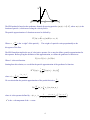
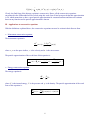
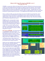
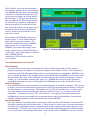
)($,QIRUPDWLRQ,QWHUQDWLRQDO1HZV
)RU7KH
:RUOGZLGH(QJLQHHULQJ&RPPXQLW\
$QQLYHUVDU\,VVXH
2FWREHU
VW
)($,QIRUPDWLRQ,QF
ZZZIHDLQIRUPDWLRQFRP
1
)HDWXUHG$UWLFOHV
FEA Information
International News:
Managing Editor
Trent Eggleston
Feature Editor
Marsha Victory
Technical Writer
David Benson
Art Director
Wayne Mindle
The contents of FEA
Information International
News is deemed to be
accurate and complete.
However, FEA Information
Company doesn’t guarantee
or warrant accuracy or
completeness of the
material contained in this
publication.
All trademarks are the
property of their respective
owners.
FEA Information
International News is
published for FEA
Information Inc..
© 2001 FEA Information
Inc. International News. All
rights reserved. Not to be
reproduced in hardcopy or
electronic format without
permission of FEA
Information Inc..
Pg
Featured Articles
03
Smoothed Particle Hydronamics – Part I of II
Jean Luc Lacome, LSTC
07
Editing LS-DYNA Input Files using Oasys PRIMER Version 8.1
12
History & Future of Computing – FAQ Part 3 of 3
Paul Bemis, ANSYS
14
Contact Modeling in LS-DYNA part 3 of 4
Suri Bala, LSTC
17
Eta/FEMB27-PC
Armando Esteves, ETA
19
FEA Information Inc. World Wide Participant Introduction:
The Japan Research Institute, Limited
20
Courses & Events
21
Web Site Summary
22
Monthly Product Showcase
DO NOT OPEN e-mail from:
feainformation.com
FEA Information Inc. ONLY uses
[email protected]
[email protected]
2
Smoothed Particle Hydrodynamics – Part I of II
© Copyright, Dr. Jean Luc Lacome 2001
INTRODUCTION
Smoothed Particle Hydrodynamics (SPH) is an N-body integration scheme developed by Lucy, Gingold and
Monaghan (1977). The method was developed to avoid the limitations of mesh tangling encountered in
extreme deformation problems by the conventional finite element method. The uniqueness of SPH is the
absence of background grids. Therefore, partial differential equations, such as conservation laws, are
transformed into integral equations. The kernel estimate then provides approximation functions to estimate
field variables at discrete points. This paper is devoted to the presentation of this method. The first part will
introduce the foundational theories of this method. In part II, we will present the development of this new
feature in LS-DYNA and the coupling method for SPH and the finite element method.
I - Definitions
The particle approximation of a function is:
Π h f ( x) = ∫ f ( y )W ( x − y, h)dy
Where W is the kernel function.
The Kernel function W is defined as:
W (x, h) =
1
θ ( x)
h( x ) d
Where d is the number of spatial dimensions and h is called smoothing length which varies in time and in
space, and x is the location of the particle.
Usually, W (x, h) is a centrally peaked function. The common smoothing kernel θ used by the SPH community
is the cubic B-spline.
1− 3 u + 3 u
 2 4
θ(u)=C× 1 (2−u)
4
0

for
0/u / ≤1
for 1≤ /u / ≤2
else
Where C is a constant of normalization that depends on the number of spatial dimensions.
3
W
x
-4
-2
0
2
4
The SPH method is based on the quadrature formula for moving particles ((x i (t )) i ∈ {1..N } , where x i (t ) is the
location of particle i, which moves along the velocity field v.
The particle approximation of a function can now be defined by:
N
Π h f (x i ) = ∑ w j f (x i )W (x i − x j , h)
j =1
Where w j =
mj
is the “weight” of the particle j. The weight of a particle varies proportionally to the
ρj
divergence of the flow.
The SPH formalism implies the use of a derivative operator. So we need to define a particle approximation for
this operator. Before giving the definition of this approximation, we define the gradient of a function as:
∇f ( x) = ∇f ( x) − f ( x)∇1( x)
Where 1 is the unit function.
Starting from this relation, we can define the particle approximation of the gradient of a function:
N
Π h ∇f (x i ) = ∑
j =1
where Aij =
1
h
d +1
θ ’(
// xi − x j //
h
mj
ρj
[ f (x ) A
j
ij
− f (x i ) Aij
)
We can also define the particle approximation of the partial derivative
Πh (
∂
:
∂xα
N
∂f
)(
x
)
=
w j f (x j Aα (x i , x j )
∑
i
α
∂x
j =1
where A is the operator defined by : A( xi , x j ) =
α
]
h
d +1
 // xi − x j //
( xi − x j )
1
θ ’ 
( xi ,x j ) // xi − x j //  h( xi , x j )
A is the α -th component of the A vector.
4



II - Discrete form of conservative equations
We are looking for the solution of the equation:
Lv (φ ) + divF (x, t , φ ) = S
where φ ∈R d is the unknown, F β with β ∈ {1..d } represents the conservation law and Lv is the transport
operator defined by:
Lv :φ → Lv (φ ) =
•
∂φ d ∂ ( v lφ )
+∑
∂t l =1 ∂x l
The strong formulation approximation:
For the strong form solution, the equation is kept at its initial formulation. The discrete form of this equation
implies the definition of the operator of derivation D defined by:
D :φ → Dφ ( x) = ∇φ ( x) − φ ( x)∇1( x)
The particle approximation of this operator is:
N
Dhφ (x i ) = ∑ w j (φ (x j ) − φ (x i )) Aij
j =1
where Aij is defined previously.
Finally, the discrete form of the strong formulation is written:
d
( wiφ ( x i )) + wi Dh F ( x i ,t ,φ ) = wi S ( x i )
dt
However this discrete form is not conservative; therefore the strong formulation approximation is not
acceptable for the numerical computation. Thus, we are compelled to use the weak form.
•
The weak formulation approximation :
In the weak form formulation, the adjoint of the Lv operator is used:
L*v :φ → L*v (φ ) =
d
∂φ
∂φ
+ ∑ vl l
∂t l =1 ∂x
The discrete form of this operator corresponds to the discrete formulation of the adjoint of Dh, s :
N
Dh*,sφ (x i ) = ∑ w j (φ (x i ) Aij − φ (x j ) A ji )
j =1
A discrete adjoint operator for the partial derivative is also necessary, and is taken to be the α − th component of
the operator:
5
N
Dα*φ (x i ) = ∑ w jφ (x j ) Aα (x i , x j ) − w jφ (x i ) Aα (x j , x i )
j =1
Clearly, the final form of the discrete equation is conservative. Hence, all the conservative equations
encountered in the SPH method will be solved using this weak form. It has been proved that this approximation
is P0, which means that we have a good particle approximation for constant functions and that error estimate
between any function and its particle approximation is known.
III - Applications to conservative equations
With the definitions explained above, the conservative equations can now be written in their discrete form.
•
Momentum conservation equation :
The momentum equation is:
dv α
1 ∂ (σ αβ )
(x i (t )) =
(x i (t ))
dt
ρ i ∂xi
where α , β are the space indices, v is the velocity and σ is the stress tensor.
The particle approximation of the weak form of this equation is:
N
σ α ,β ( x j )
σ α ,β ( x i )
dv α
( xi ) = ∑ m j (
Aij −
A ji )
dt
ρ i2
ρ 2j
j =1
•
Energy conservation equation :
The energy equation is:
dE
P
= − ∇v
dt
ρ
where E is the internal energy, P is the pressure and ρ is the density. The particle approximation of the weak
form of this equation is:
P
dE
(x i ) = − i2
dt
ρi
N
∑ m (v ( x
j
j =1
6
j
) − v(x i )) Aij
Editing LS-DYNA Input Files using Oasys PRIMER Version 8.1
© Copyright Oasys, 2001
PRIMER is a pre-processor dedicated to editing LS-DYNA input files. While there are many pre-processors
available for mesh-building and general modeling, their support for non-linear input data is often incomplete:
specialist data such as load-curves, joints, complex material models and so on can be lost when an existing
analysis is taken back into them for modification, or when models are merged. In addition there are several
specialist functions peculiar to particular types of analysis, such as occupant positioning, which are not provided
satisfactorily by general-purpose pre-processors. Oasys PRIMER has been designed to solve these problems.
Primer is capable of reading, processing and writing out the entire LS-DYNA keyword input deck, with no
exceptions or omissions: no information is lost during processing. It will also read and write several other
common formats. Input decks may be visualized directly, and any number of input models may be merged
intelligently into a single output model; with the additional ability to translate, rotate, reflect and scale models,
parts or individual components in the process.
PRIMER provides several specialist occupant
modeling features. It will manipulate occupant
(dummy) models intelligently, providing easy
interactive positioning of whole models and their
constituent parts; it will fold airbags; it will fit
seatbelts. This positioning, folding and fitting
information is appended to the end of the output
deck, and can be reread back in directly for further
manipulation if required.
The Purpose of PRIMER: The standard approach
to using PRIMER is illustrated in Figure 1. A
general purpose pre-processor is used to create the
Finite Element mesh from CAD data. Primer
imports the mesh where all of the many LS-DYNA
specific features can be added. In addition to
editing these features, PRIMER aids the user by
visualizing them and providing detailed crossreferencing from feature to feature. Both by using
the edit menus and by using Find Attached.
Figure 1 The Purpose of PRIMER
Further data can be combined with the model from
other sources such as the Bill of Materials,
Materials Database and Spotweld file. The required
mass can be applied to the model using the Massing
function. Other models can be combined at this
point. One of the original reasons that PRIMER
was developed was to assist in merging Occupant
models, handling the issues related to positioning,
contact definition and seatbelt fitting. Finally, the
model can be checked, with over 1500 separate
checks carried out as well as new functions to check
contact penetration, mass scaling requirements.
PRIMER provides checks of material and section
properties using contour plotting.
Figure 2 Typical model modification process
7
While all this is very useful when preparing a
new model for analysis, there are more reasons
why PRIMER should be used when modifying
a model for second and subsequent runs. The
typical process to modify an existing model is
shown in Figure 2. Most pre-processors lose
data on reading the LS-DYNA model because
not all features are supported. Although it is
sometimes possible to re-stitch this lost data
back in after the model is written again (one of
the great benefits of the Keyword format of
course), mistakes can be made and a lot of
time can be wasted.
The procedure with PRIMER is improved, as
shown in Figure 3. Mesh modifications are
made in the pre-processor as before. The
model to be modified is read in by PRIMER
along with the new or modified mesh;
PRIMER’s powerful model merging is then
used to combine the two with full checking to
avoid clashes. Any further changes can then be
made in PRIMER before
writing the LS-DYNA model, ready for
a new analysis.
Figure 3 Model modification process with PRIMER
New Modelling Features in Version 8.1
Bill of Materials:
It can be difficult to ensure that a crash model is up to date with the latest product release; material
properties and gauge can change for existing parts, and parts can be added or deleted. This information is
summarized in the Bill of Materials (BOM) which is usually maintained as a spreadsheet. PRIMER is now
able to read this spreadsheet. By matching names between BOM and model PRIMER can be used to ensure
that the model is up to date. After reading the spreadsheet, the user must define the meaning of each data
column, e.g., Part ID number, material name, gauge, etc. PRIMER then checks the model against the
spreadsheet and reports any errors, including parts in the BOM that are not in the model and vice-versa.
Materials Database:
Once the BOM has been read, the materials for each matching part are renamed accordingly. This name can
be used to extract the required material properties and values from an existing material database, created by
the individual user or system manager. The database is in LS-DYNA Keyword format. As long as some
part of the model material name matches the database, a match will occur; e.g., a material name “CR4
Treatment C” will match one named “CR4” in the database. After applying, all matched materials are
highlighted; the user may then modify the selection and choose values from the database for unmatched
materials. Multiple databases can be created and selected within PRIMER.
Spotweld Definition:
One of the most time-consuming tasks in constructing a vehicle model is the definition of the thousands of
spotwelds connecting the body-in-white panels. Up until recently it was necessary for spotweld elements to
join nodes in the panel flanges directly, forcing the model to have carefully matched mesh densities on all
mating flanges. LS-DYNA, from Version 950, has offered mesh independent spotwelds with the potential
to save a great deal of time during mesh creation. Now with the release of PRIMER 8.1, the user can take
8
full advantage of mesh-independent
spotwelds as almost all of the hard work in
creating the required nodes, beams, materials
and tied contact surfaces has been eliminated.
Individual spotwelds can be quickly created
by the user. After defining which panels are
to be joined, the user only needs to select one
node and all the rest is automatic. A second
node is projected onto the mating flange and
a beam created between them; for a weld
through three or more layers, PRIMER will
create a chain of beams. The beam material
and section properties and the tied contact
interface required to stick the projected node
to the flange are all easily defined.
Figure 4 Reading a Spotweld file into PRIMER
Even more powerful, however, is the
ability to read a spotweld CAD file. This
file, which need only contain the x, y, z
coordinates of each weld, can be read from a
spreadsheet format. As with the BOM, the
user must define which column defines
which data. Including the panel part IDs for
the weld can also be useful as it can avoid
errors later. An example is shown in Figure
4. All possible spotwelds are created in the
model by pressing Apply once the file is
read and the columns are defined. A typical
result is shown in Figure 5.
Any spotwelds that cannot be made are
Figure 5 Spotwelds created automatically in PRIMER
reported to the user for individual editing.
Individual welds can be isolated and shown;
this may reveal that the wrong panels were
selected. Other reasons why the welds could
not be made can also be displayed. Most
often, these will relate to the maximum or
minimum length defined for a spotweld, the
minimum pitch, the angle to the panel or the
maximum number of panels that can be
joined with a single weld. Finally, Find
Connected and Find Unconnected functions
can be used to check that all relevant panels
have been successfully spotwelded.
Mass Assign:
Another new useful function for LS-DYNA
users is Mass Assign. Often parts in a model
are represented by approximate geometry, or a solid
body might just be represented by an exterior shell
Figure 6 Result of mapping forming data
element mesh. PRIMER offers the ability to smear
9
mass over these parts to obtain the required total mass and centre of gravity.
Effects of Forming:
An area gaining more and more interest is how the forming process affects the performance of the
manufactured component. Research has shown that strain hardening and thickness changes can have a
significant influence on the crash response of a vehicle, so functions have been added to PRIMER to help
users include these effects. Data from a separate forming simulation must be mapped onto the crash model;
but often the forming model will have a different mesh density and a different orientation. PRIMER tackles
this by defining an orientation based on three nodes in each model and then mapping the thickness and
plastic strain data from the forming model to the crash model. A typical result is shown in Figure 6.
Advanced Checking Functions:
PRIMER has always had the capability to check and clean up a model before saving it for analysis. For the
Version 8.1 release, even more checks have been added and a number of these now have an Autofix option.
Beyond these, several new functions have also been added to visually inspect the model and ensure that the
analysis runs “right the first time”.
Find Attached is one of the new visual
checking capabilities. This feature allows
the user to build the model entity by entity,
to ensure that the connections are intended.
PRIMER’s ability to visualize all LS-DYNA
features gives it a unique capability to
visualize the model construction.
Contact Penetration checking is another
new addition. Once a contact surface has
been defined a check can be made; PRIMER
reports the number of penetrating nodes as
well as any shells which actually cross each
other. The maximum penetration is stated
and contour plots of the depth of penetration
are available as shown in Figure 7. When
the number of penetrations is high,
individual nodes can be selected for
checking. At present the options to fix
penetrations within PRIMER are limited,
although null beam elements can be created
to help find the problem areas in a meshing
pre-processor.
Figure 7 Contour plot of contact penetration
The new contouring capability allows a number of other model characteristics to be checked in PRIMER
8.1. Values that can currently be displayed include shell thickness, material properties such as yield stress,
and element timestep and percentage added mass for mass scaling requirements (if a minimum timestep is
defined). Vector plots are also now possible. For example, initial velocity can be plotted to check that all
entities have the required velocity value (and direction) and any errors due to *PART_INERTIA definitions
can be corrected.
10
Improvements to General Functionality:
A new header bar has been added to the top of the graphics window giving rapid access to commonly used
functions, such as the draw commands (hidden line, shaded image, etc.) and the blanking menu. Some of
the new features, such as vector plots of velocity or contour plots of timestep or mass scaling, can also be
accessed from here. In addition, new options have been added to modify the appearance of the graphics
display and a bitmap output option has been added.
More options for handling the *INCLUDE keyword have been added in the latest release. More often,
modellers are using *INCLUDE to assemble large models from a library of smaller sub-models – this
provides a flexible way to manage a complex family of vehicle crash models. PRIMER now offers the
option not to read included models when the main model is imported, and offers three alternative ways of
handling the included models when writing the main file.
Finally, a new HTML help facility has been added for with all the details of the original online PDF manual but
with powerful search and jump functions; this is in addition to the text help menus in the previous version.
There is now a MANUAL button on every help window which links directly to the relevant page of the HTML
manual. Here you will find detailed explanation with diagrams and screen captures to demonstrate the use of
the function of interest. Full search and navigation functions allow the user to quickly find related information.
11
Part 3 of 3 – FAQ on Web Based Distributed Simulation
© Copyright Paul Bemis, 2001
ANSYS, Inc.
Web Based Distributed Simulation
ANSYS has been a pioneer in the area of delivering complete engineering solution systems for over 30
years. Over the past ten years, these solutions have focused primarily on the Engineering Workstation
and Personal Computer model of computing due to their outstanding cost effectivity and market
demand. However, the trend towards highly complex “real world” engineering simulation often exceeds
the capacity of these personal systems. As web based computing becomes more popular and cost
effective, the opportunity to use remote computational servers to augment the desktop systems becomes
practical. The ANSYS e-Sim strategy is focused on delivering engineering simulation solutions that can
be deployed on web based infrastructures for optimal cost effectivity and efficiency in product design
environments. The primary benefit of this strategy is by creating ANSYS products that are “web
enabled” the deployment of these solutions can be done on LANS, WANS, Intranets, Extranets, or the
worldwide web. Furthermore, they can be deployed either within one company, or across the supply
chain that services a company.
The following FAQ covers Security, Support and Performance.
Security
Generally, how secure is the e-cae.com infrastructure?
All communications between the users system and e-cae.com utilize state of the art Secure Socket Layer
SSL technology. Communication is encrypted and secure. User names and passwords are randomly
generated and unique. All operations are continuously monitored for possible misuse. The technology used
on e-cae.com provides the highest level of security in the market today. For those users who require
excellent security, private VPN or leased lines can be provided, as well as dedicated computational
systems. The hosting provider for e-cae.com is Genuity Inc (www.genuity.com) and a tour of the Genuity
facility can be arranged for customers who desire to see the security infrastructure “first hand”.
What kinds of security does e-cae.com use to protect customers data?
All customer data is protected using a scheme of unique user and password ID. Advanced security features
are used extensively throughout the site and data within e-cae.com is protected using unique naming
conventions. Under this method there is no ability for one customer to view another customers data, unless
explicitly permitted.
How can I be sure the e-cae.com solution will work with my current corporate firewall?
Provided the customer can “see” the internet, e-cae.com will be operative. There is no incremental work
required from the customers IT organization. The e-cae.com solution will use either port 80 or 443
depending whether the customer is operating in “secure” SSL or utilizing an “open” connection.
What precautions are in place to prevent an attack of the e-cae.com site?
Continuous traffic monitoring is in place on a 7x24x365 basis providing the highest degree of pro-active
protection available today. Procedures used leverage state of the art technologies and methods to provide
extensive security capability.
Will e-cae.com provide a virtual private network (VPN)?
Yes, please ask ANSYS Inc reseller or partner for pricing. VPN’s are available for an added level of
security in most geographies worldwide.
12
Support
How does the support model work?
Support for ANSYS users is provided in the same model as today. ANSYS customers typically purchase
through an ANSYS Support Distributor in their local region. This same organization is responsible for the
support of the e-cae.com offerings.
Does e-cae.com supply clear reports with detailed application access and usage statistics?
Yes, the reporting capabilities of e-cae.com are quite extensive. Users can access reports online that include
parameters such as number of file transfers, number of CPU hours, number of logins, and other data of
interest. Customer site administrators have more reporting features including the above statistics for
multiple users and/or multiple sites within the customers company.
How does e-cae.com manage the ANSYS version or release migration?
Yes, e-cae.com completely manages application migration for the customer. This includes the rapid “same
day” introduction of new ANSYS releases and patches, as well as the operation of older versions of
ANSYS for users requiring revision compatibility with installed base application revisions.
What happens when a job that has been submitted hangs, or crashes?
ANSYS has developed a customer support process that will determine the reason for the problem, and
appropriate resolution. In cases where it is determined to be an issue with the ANSYS program, a
proportionate amount of CPU time will be credited to the customer account.
Performance
How fast is e-CAE.com compared to my local computer?
The answer to this will largely depend on the configuration of the local computer, as well as the size and
type of simulation being run. However, in test comparisons between the e-CAE.com service and a local
PC operating at 800Mhz, the e-CAE.com server is delivering solutions nearly 3x faster for static analysis
in the range of 100K DOF using one CPU. Additionally, when operating ANSYS in parallel mode on eCAE.com, the time to solution will decline proportionately as processors are applied to the solution.
For pricing and further information contact: Paul Bemis, [[email protected]] the author of this series
article and the manager of The ANSYS, Inc. e-CAE.com ASP Program that provides:
•
A mechanism for running ANSYS simulations and/or LS-DYNA simulations on large parallel
compute servers, at a remote data center site using the internet.
• A system that has been developed to allow engineers the ability to run remote simulations with
specific controls on job execution parameters.
• A solution that uses “state of the art” security and systems infrastructure technology from providers
including Sun, Hewlett Packard, Silicon Graphics, Cisco, and others.
• A service that is ideal for engineers and companies requiring occasional “surge” capacity for time
critical simulations, or periodic simulations of large models.
Key e-CAE.com seccurity features:
• HTTP or HTTPS (Secure) access
• Strict account & file controls.
• Full data communication encryption.
• Secure Socket Layer (SSL).
• Continuous monitoring on all operations.
13
Contact Modeling in LS-DYNA
© Copyright LSTC – Suri Bala, 2001
Part 3 - Modeling Guidelines For Full Vehicle Contact
Upcoming issue Part 4:
Airbag Contact, Edge-to-Edge Contact, and Rigid Body Contact
7.0
Modeling Guidelines For Full Vehicle Contact
Crash analysis involving a full vehicle incorporates contact interactions between all free surfaces. This
is quite expensive since 20-30 percent of the total calculation CPU time is used by the contact treatment. One
of the challenging aspects of contact modeling in crash analysis is the handling of interactions between
structural metallic parts and non-structural components typically made from foam and plastic. This is especially
important when occupants are included in the model. Another challenge is handling contact at corners or edges
of geometrically complex parts. Guidelines should be followed to achieve stability in contact as well as
reasonable contact behavior. Some of the modeling practices based on experience are discussed below.
7.1
Global or Local Contact
Historically, many individual contact definitions were used for the treatment of contact. The
development and implementation of a robust single surface type of contact has changed the way engineers
model the contact today. From the standpoints of simplicity in preprocessing, numerical robustness, and
computational efficiency, it is now usually advantageous to forsake the use of numerous contact definitions in
favor of ONE single-surface-type contact that includes all parts which may interact during the crash event. We
often casually refer to this single contact approach as a global contact approach.
This, however, does not mean that one should always avoid local contact definitions. Frequently, there
exist certain areas of the vehicle that require special contact considerations where the global contact definition is
observed to fail. In such instances the user is encouraged to define local contact interfaces with non-default
parameters that would best suit the contact condition.
7.2
AUTOMATIC_SINGLE_SURFACE or AUTOMATIC_GENERAL
Though both contact algorithms belong to the single surface contact type, several key parameters
distinguish these two contact types. Table 7.1 highlights the important differences.
PENMAX
AUTOMATIC_SINGLE
SURFACE
0.4
BSORT frequency
Every 100 cycles
Every 10 cycles
SEARCH DEPTH
2
3
Shell Exterior Edge Treatment
No
Yes
Beam to Beam Contact
No
Yes
Parameters
Table 7.1
AUTOMATIC_GENERAL
100
Difference Between AUTOMATIC_SINGLE_SURFACE (13) and
AUTOMATIC_GENERAL (26)
14
Of the two single surface contact types listed in Table 7.1, *AUTOMATIC_GENERAL is
computationally more expensive owing to its additional capabilities and its more frequent and thorough contact
search.
The AUTOMATIC_SINGLE_SURFACE contact option is recommended for global contact. To treat
special contact conditions where shell edge-to-edge or beam-to-beam contact is anticipated, the additional use
of the AUTOMATIC_GENERAL contact in localized regions is recommended. AUTOMATIC_GENERAL
contact should be used sparingly and only where conditions dictate its use. One advantage of the
AUTOMATIC_SINGLE_SURFACE contact starting with LS-DYNA version 950d is in its more rigorous
treatment of interior sharp corners within the finite element mesh and in the handling of triangular contact
segments; consequently, the AUTOMATIC_SINGLE_SURFACE contact is usually superior for parts meshed
from triangular and tetrahedron elements. In future version of LS-DYNA, the AUTOMATIC_GENERAL
option will also include these improvements.
7.3
Standard Penalty-Based or Soft Constraint Stiffness Method
When several parts of dissimilar mesh sizes and/or dissimilar material properties are included into one
global slave set for AUTOMATIC_SINGLE_SURFACE, the soft constraint stiffness method (SOFT =1) is
recommended. The soft constraint method seeks to maximize contact stiffness while also maintaining stable
contact behavior. The interacting nodal masses and the global time step are used in formulating the contact
stiffness. The segment-based contact method, invoked by setting SOFT=2, calculates contact stiffness much
like the soft constraint method but otherwise is quite different. Segment-based contact can often be quite
effective where other methods fail at treating contact at sharp corners of parts.
In contrast to a soft constraint approach, the standard penalty-based contact stiffness (SOFT=0) is based
on material elastic constants and element dimensions. In foam and plastic materials, the contact stiffness given
by the two methods can differ by one or more orders of magnitude. The primary disadvantage of choosing the
soft constraint method is its dependence on the global time step. Occasionally, the global time step must be
scaled down using the TSSFAC parameter in *CONTROL_TIMESTEP to avoid numerical instabilities in the
contact behavior. This results in an increased run time for the entire simulation. As an alternative to reducing
the global time step the soft constraint scale factor, SOFSCL, in the *CONTACT definition can be reduced
from the default value of 0.1 to 0.04-0.07.
If the standard penalty-based approach in used in a global contact definition, the soft constraint approach
can be used locally to handle dissimilar materials in contact. The following are examples where contact
behavior may benefit from use of the soft constraint method:
• Airbag to Steering Wheel
• Airbag to Occupant
• Front Tire to SIL
• Spare tire to neighboring components
• Foam to structural components
Using a combination of both contact stiffness methods may promote good contact behavior without having to
reduce the global time step.
7.4
Definition of Slave Set
There are several ways to define the slave set for the global contact definition. These include: all parts
(this is the default), a set of included parts, a set of excluded parts, or a set of segments. The default, which
includes all parts, can sometimes result in obvious instabilities at the beginning of a simulation unless great care
is taken in setting up the model to avoid such things as initial penetrations and nonphysical intersections of
parts. The option to ignore penetrations on the *CONTROL_ CONTACT keyword (set IGNORE equal to 1) is
recommended if care is not taken to eliminate initial penetrations. Many models run perfectly with just one
15
interface definition; others, however, will not run until changes are made to the input, usually by excluding parts
or by modifying the finite element mesh to more accurately reflect the physical model.
To reiterate, the following methods can be used for defining the global contact definition:
• All parts (default)
• Included parts by *SET_PART
• Excluded parts by *SET_PART. Non-Excluded parts will be considered for contact
• Segments by *SET_SEGMENT
In addition to the above slave sets, a three-dimensional box, defined using *DEFINE_BOX, may be
used to restrict the contact to the parts or segments that lie within the box at the start of the calculation. This will
reduce the extent of the contact definition leading to a reduction in contact-associated cpu time.
7.5
Friction
When using one global contact that includes several components of the vehicle, a uniform friction
coefficient (possibly zero) may be acceptable for initial analyses. However, the use of *PART_CONTACT
keyword to specify friction coefficients on a part-by-part basis is recommended when friction is expected to
play a significant role. Friction coefficients specified in *PART_CONTACT will override friction coefficients
specifed elsewhere if and only if FS in *CONTACT is set to –1.0. Please note that the dynamic friction
coefficient FD will have no effect unless a nonzero decay coefficient DC is provided.
7.6
Contact Thickness
To reduce the number of initial penetrations, the contact thickness can changed from the default element
thickness by using the global SST and MST parameters in *CONTACT. The OPTT parameter in
*PART_CONTACT can be used to override SST and MST on a part-by-part basis. The user is cautioned
against setting the contact thickness to an extremely small value as this practice will often cause contact failure.
In fact, for treating contact of very thin shells, e.g., less than 1 mm, it may be necessary to increase the contact
thickness to prevent contact failure.
If a contact surface is comprised of tapered shell elements, then a uniform contact thickness should
always be specified. The contact assumes that the segment thickness is constant, which can result in thickness
discontinuities between adjacent segments. As a node moves between segments of differing thickness, the
interface force will either suddenly drop or increase as a result of the discontinuous change in the penetration
distance. This can result in negative contact interface energies.
16
eta/FEMB27-PC
Finite Element Model Builder, version 27 for PC © Copyright, 2001
Armando Esteves, ETA
eta/FEMB27-PC is the newly released version of ETA’s pre-/post-processor for LS-DYNA for personal computers
using Windows 98/NT4/2000. More than a regular upgrade, eta/FEMB27-PC was redesigned from the ground up
based on the Unix version of eta/FEMB which is 100% compatible with LS-DYNA.
Complete LS-DYNA Interface: The major goal in the development of eta/FEMB27-PC was to fully support LSDYNA in a non-text-editing environment. To reach this goal, the following requirements were defined:
• support all LS-DYNA cards and keywords (graphical and numerical);
• set default values as in the LS-DYNA User’s Manual and input validation check;
• total graphical interface;
• remain user-friendly and intuitive;
• maintain efficiency and high performance;
• remain the most cost-effective solution available to users.
During development of eta/FEMB27 for unix workstations, ETA designed an “LS-DYNA Template” which allows
our developers to easily keep pace with the evolution of LS-DYNA and the release of new keyword commands. A
simple addition to our text-based template enables almost immediate compatibility with new or enhanced features
of LS-DYNA. In eta/FEMB-PC Version 26, LS-DYNA capabilities were hardcoded into the software, making it
difficult to keep up with solver development. To respond effectively to user needs, it was essential to port the
LS-DYNA Template to eta/FEMB-PC. This was the primary motivation for a completely new interface. With the
advent of the LS-DYNA template, we can also provide the default values as defined in the User’s Manual and
perform an input validation check according to the expected value range and numerical format.
The introduction of the LS-DYNA Template generates a graphical entity named “LS-DYNA Data Table/Collector”
(Fig. 1).
Fig. 1: LS-DYNA Data Table/Collector
The LS-DYNA Data Collector is a graphical and intuitive version of the command descriptions in the LS-DYNA
User’s Manual. It graphically provides the keyword command, the number of cards associated with it, the variable
name on each card, a brief description, and a value field for data input and default value (if any). It provides the
user with an electronic version of the LS-DYNA User’s Manual embedded in the pre-processor interface. Sample
windows with the extensive list of Material Keywords (Fig. 2) and the available Contact Keyword selection (Fig. 3)
are shown on the next page.
Redesign of the eta/FEMB27-PC started by determining the best way to handle the large amount of data necessary
to build an LS-DYNA model. We borrowed from the UNIX version to design the new GUI. We feel that the new
design has made the GUI even more organized and intuitive. The fact that the new GUI resembles the UNIX
version allows for a smooth transition to the new PC version.
17
Fig. 2: Structural Material Keyword list
Fig. 3: 3D Contact Keyword List
Productivity is improved by easy command access through function keys and model handling is enhanced with
mouse and keyboard combinations. Model handling is also better due to the introduction of mouse drag zoom.
The menus are reorganized in a logical way (File / CAD / Model / Properties) and the tools icon menus are preemptive. The simple interface eliminates the steep learning curve normally associated with a full featured
program.
eta/FEMB27-PC has extensive CAD capabilities which cover the line and surface definition needs of most
power users. Also, more robust IGES and VDA input translators are now available. A powerful new feature is
the ability to generate curves (or, load curves) directly from a new graphic plot handler. Curves can be input or
inserted (read from a table) in various ways and are immediately associated with the loading case.
eta/FEMB27-PC contributes to model data discussion by providing direct export of model images to JPEG
format which can be easily inserted into documents, presentations or posted on the Internet. eta/FEMB27-PC
allows direct export of the LS-DYNA model to virtual reality VRML format, allowing anyone to manipulate the
3D model using an internet capable browser.
Eta/FEMB27-PC, Compete LS-DYNA Solution Package: Although “FEMB” has historically been
perceived as only a pre-processor, eta/FEMB27-PC is in reality a complete LS-DYNA solution package that
includes:
• FEMB, pre-processor;
• PostGL, post-processor (d3plot);
• eta/Graph, plot post-processor (ASCII and binary).
Cost-Effective Solution: ETA foresaw the current trend and began several years ago to make the transition
from Unix platforms to more cost-effective personal computers. Our goal has been to achieve the same features
and ease of use in eta/FEMB27-PC that have been the hallmark of our workstation version.
18
With our 1st anniversary issue of FEA Information News
we are pleased to Showcase one of our participating companies
The Japan Research Institute, Limited
www.jri.co.jp
(excerpt from the website: The Japan Research Institute, Limited)
Information technology (IT) is at the heart of a broad process that is radically transforming industry and
society not only in Japan but on a worldwide scale. To survive this age of rapid change requires sound
business management based on a clear vision of the future and well-thought-out strategies for information
utilization. Since its establishment, The Japan Research Institute, Limited (JRI) has kept pace with its clients
and their changing needs by basing our operations on the underlying principle of "creating new value for
clients." That is, by identifying problems hindering companies and offering concrete, practical proposals for
solving those problems, JRI generates new arenas of value for its clients to explore. At JRI, these efforts
toward comprehensive problem-solving are understood as "knowledge engineering," a concept which forms
the foundation of all our activities.
Offices
Head Office
Osaka Head Office
Branch Offices
Representative Office
Computer Centers
16 Ichiban-cho, Chiyoda-ku, Tokyo 102-0082, Japan
TEL: (81)(3)3288-4700
5-8 Shinmachi 1-chome, Nisi-ku, Osaka 550-0013
TEL: (81)(6)6534-5111
Sapporo, Nagoya, Fukuoka, New York, Singapore
Hong Kong
Tokyo, Higashi Nihon, Gokokuji, Yotsubashi, Kinyu-kyodo
Products for Engineering LS-DYNA
Nonlinear Dynamic Analysis of Structures
JOH/NIKE 2D/3D
An implicit Finite-Deformation Finite Element Code
JMAG-Works – JMAG Studio
Electromagnetic Analysis Software
JVISION
Pre-post Processor
JSTAMP-WORKS
A sheet metal forming simulation system
19
FEA Information Web Sites Monthly Summary
September articles are archived on the News Page at www.feainformation.com
Articles from September on FEA Information website
Sept. 03
Sept 10
Sept. 17
Sept 24
New Site
High Performance Computing Servers (www.hpcservers.com)
Software
PostGL 1.0 from Engineering Technology Associates
Software
OASYS T/HIS from OASYS, Ltd
Software
LMS Roadrunner from LMS Int’l
Hardware
hp 9000 unix servers from Hewlett-Packard
Software
EASI-SEAL® from EASi Engineering
Distributor
Engineering Research AB [ERAB] located in Sweden
Product
LifeBook notebook series from Fujitsu Ltd
Software
LS-POST free post processor from Livermore Software Technology Corp
Distributor
THEME Engineering, Inc. located in Korea
Software
MSC.Linux version August 2001 from MSC Software
Software
JOH/Nike 2D/3D from The Japan Research Institute
Distributor
Metal Forming Analysis Corp. [MFAC] located in Canada
I would like to take this opportunity to thank everyone for helping us publish a monthly publication for the past
year.
A special thanks to Desktop Engineering Magazine, a Helmers Publishing Inc. publication,
www.deskeng.com for allowing FEA Information News to reproduce their articles relating to FEA Information
Participants.
In coming issues we will have articles in reference to our engineering websites:
• High Performance Computing Servers: www.hpcservers.com - has information online and is
scheduled to be fully operational February 2002.
• Meshless Methods: www.meshlessmethods.com - will be operational February 2002
• Fluid-Structure Interaction: www.fluid-structureinteraction.com - has information online and is
scheduled to be fully operational February 2002
Future articles in the news will correlate with our numerous engineering applications websites such as:
• Heat Transfer Analysis – www.heattransferanalysis.com
• Implicit FEA – www.implicitfea.com
• Linux for PC – www.linuxforpc.com
Marsha Victory,
President, FEA Information Inc.
20
Courses and Events will be limited to 1 page
For further information contact event/course sponsor
Events/Conferences
2001
Oct 30-31
Japan Nov. 13-14
France April 22-24 May 19-21, 2002
USA LS-DYNA Users Conference, sponsored by Japanese Research Institute (JRI) - to be held
at the Sheraton Grande Tokyo Bay Hotel.
LMS 2001 Conference for Physical and Virtual Prototyping, to be held at Hotel New York,
Disneyland Paris, Paris, France. If you have any questions, contact Kirsten Cabergs, via email ([email protected]) or phone (+32-16-384-200). ANSYS Users Conference & Exhibition 2002 - Pittsburgh Hilton, Pittsburgh, PA. For
information visit: ANSYS, Inc. 7th International LS-DYNA User’s Conference at the Hyatt
Regency Hotel & Conference Center - Fairlane Town Center,
Dearborn, MI 48126
Hyatt Regency Hotel & Conference Center
Due to the amount of travel/classes/conferences being rescheduled
I have listed the websites of our FEA Information Participants
for you to visit for up to date information
Headquarters
USA
USA
UK
Japan
USA
USA
USA
USA
Japan
USA
Belgium
Sweden
USA
Korea
Korea
Australia
Canada
France
India
Russia
Company
Livermore Software Technology
Engineering Technology Associates
OASYS, Ltd
The Japan Research Institute, Ltd
ANSYS, Inc
Hewlett Packard
SGI
MSC Software
Fujitsu Ltd.
EASi Engineering
LMS, International
Engineering Research AB
DYNAMAX
THEME Engineering
Korean Simulation Technologies
Leading Engineering Analysis Providers
Metal Forming Analysis Corp.
Dynalis
GissEta
Strela – Russia
21
website
www.lstc.com
www.eta.com
www.arup.com /dyna
www.jri.co.jp
www.ansys.com
www.hp.com
www.sgi.com
www.mscsoftware.com
www.fujitsu.com
www.easiusa.com
www.lmsintl.com
www.erab.se
www.dynamax-inc.com
www.lsdyna.co.kr
www.kostech.co.kr
www.leapaust.com.au
www.mfac.com
www.dynalis.fr
www.gisseta.com
www.ls-dynarussia.com
)($,QIRUPDWLRQ6KRZFDVH
The Japan Research Institute Limited
www.jri.co.jp/pro-eng/jmag/e/jmg/index.html
JMAG-Studio
A magnetic field analysis program
This example shows how JMAG can be used for
the analysis of an eddy current brake for railcars
Product names referenced herein are trademarks of their respective owners
22