Download DYNAFORM 5.0

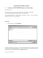
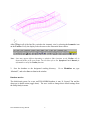
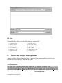
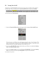
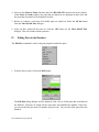
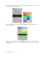
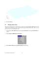
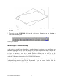
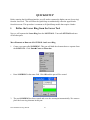
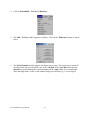
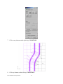
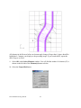
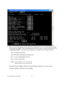
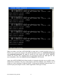
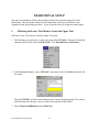
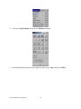
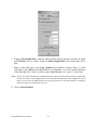
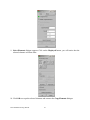
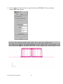
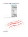
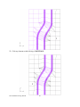
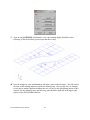
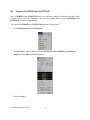
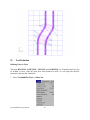
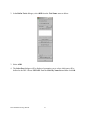
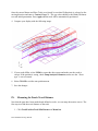
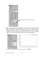
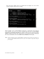
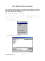
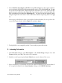
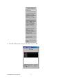
DYNAFORM 5.0
Training Manual
Version 5.0
Engineering Technology Associates, Inc.
1133 E. Maple Road, Suite 200
Troy, MI 48083
Tel: (248) 729-3010
Fax: (248) 729-3020
June 10, 2003
By: Jeanne He
TABLE OF CONTENTS
Introduction …………….……………………..Page 3
Database Manipulation….…………………….Page 4
Meshing………………….……………………Page 13
QuickSetup……………….…………………...Page 21
Traditional Setup………….…………………..Page 38
Post processing………………………………..Page 69
Conclusion……………….……………………Page 80
DYNAFORM Training Manual
2
INTRODUCTION
Welcome to the DYNAFORM 5.0 Training Manual. DYNAFORM5.0 is the unified version of
the DYNAFORM-PC and Unix platforms. This manual is meant to give the user a basic
understanding of finite element modeling for forming analysis, as well as displaying the forming
results. It is by no means an exhaustive study of the simulation techniques and capabilities of
DYNAFORM. For more detailed study of DYNAFORM, the user is urged to attend a
DYNAFORM training seminar.
This manual details a step-by-step sheet metal forming simulation process through traditional
finite element (FE) modeling and the newer QuickSetup interface process. Users should take the
time to learn both setup processes as each has inherent benefits and limitations.
The traditional setup procedure is extremely flexible and can be used to setup any forming
simulation. Because the QuickSetup makes certain assumptions as to the type of tooling
configuration selected it is not as flexible, however, it automates many of the procedures
required for traditional model setup such as travel curves.
The following table outlines the major differences between the QuickSetup and the traditional
DYNAFORM setup procedure.
QuickSetup
Traditional
Automated interface limits flexibility
Manual interface can duplicate any tooling
configuration; pads, multiple tools, etc
Requires more setup time
Manual definition of travel curves
Geometrical Offset
Reduces modeling setup time
Automated travel curves
Contact Offset
Note: This manual is intended for the application of all DYNAFORM platforms. Platform
interfaces may vary slightly due to different operating system requirements. This may cause
some minor visual discrepancies in the interface screen shots and your version of DYNAFORM
that should be ignored
DYNAFORM Training Manual
3
DATABASE MANIPULATION
I.
Creating an eta/DYNAFORM Database and Analysis Setup
Start Dynaform 5.0.
For workstation/ linux users, enter the command “df50” (default) from a UNIX shell.
For PC users, double click the Dynaform 5.0 Icon from the desktop.
After starting eta/Dynaform, a default database Untitled.df is created.
importing CAD files to the current database.
Users will begin by
Import files
1. From the menu bar, select FileÜ
Ü Import.
Change the file format to “Line Data”. Go to the training input files located in the CD provided
along with the DYNAFORM installation. Locate two line files: die.lin and blank.lin. Then,
import both files and select OK to dismiss the Import File window.
DYNAFORM Training Manual
4
After reading in all of the line files, switch to the isometric view by selecting the Isometric icon
on the Toolbar. Verify the display looks the same as the illustration shown above.
Note: Icons may appear different depending on platform. Other functions on the Toolbar will be
discussed further in the next section. You can also refer to the Dynaform User’s Manual for
information on all of the Toolbar functions
2. Save the database to the designated working directory.
“dftrain.df”, and select Save to dismiss the window.
Go to FileÜ
Ü Save as , type
Database metrics
The default unit system for a new eta/DYNAFORM database is mm, N, Second, Ton and the
draw type is double action (toggle draw). The user is able to change these default settings from
the Setup/Analysis menu.
DYNAFORM Training Manual
5
File Types
Dynaform has the ability to read the following types of input files:
8.
9.
10.
11.
12.
13.
14.
II.
Abaqus (*.inp)
Binary (*.bin)
LS-DYNA (*.dyn, *.mod)
F-crash (*.fcr)
NASTRAN (*.nas)
Pamcrash (*.pc)
Radioss (*.rad)
1.
2.
3.
4.
5.
6.
7.
Line Data (*.lin)
Iges (*.igs, *.iges)
VDA (*.vda)
DXF (*.dxf)
LS-Nike 3D (*.nik, *.mod)
DYNAIN File (*.din)
UG Part (*.prt)
Practice Some Auxiliary Menu Operations
After successfully reading in the needed files to begin the finite element modeling, practice to get
familiar with some of the basic functions and menus.
View Manipulation
View Manipulation
DYNAFORM Training Manual
6
The view manipulation area of the Toolbar is one of the most visited spots in eta/DYNAFORM.
These functions enable the user to change the orientation of the display area. Place the mouse
pointer over each icon to display the name and function of each icon. Also, take notice of the
Display Option window (shown below) at the bottom of the screen. This is another area
enabling the user to manipulate the display area.
The following steps will help you become more familiar with the functions found in the
Toolbar, and in the Display Option window.
1. Select Isometric from the Toolbar. This places the displayed geometry in an isometric
view, as shown earlier.
2. Rotate the geometry dynamically about the z-axis approximately 90° by using the Rotate
about Z-Axis function. The function is shown below:
3. Select Rear View (YZ Plane). The result is shown below:
4. Select Fill from the Toolbar, this makes the displayed geometry fill the screen.
5. Practice using the other viewing options before moving on.
DYNAFORM Training Manual
7
III.
Turning Parts On/Off
All geometry in eta/DYNAFORM is based on parts. Every entity, by default, will be created or
read into a part. The user should practice using the On/Off function, located in the Toolbar,
or in the Parts menu: Parts/Turn On.
1. Notice the Turn On/Off Part dialogue that appears after selecting the Part On/Off button.
Place the cursor over different icons and buttons to learn the name of each function. This
type of selection menu is common to the eta/DYNAFORM environment. It provides several
different functions for selecting which parts will be turned off or on.
2. Since the part BLANK.LIN contains only line data, you will have to use either the Select by
Line or the Select by Name function.
3. First, use the Select by Line icon to turn off the part, BLANK.LIN. Click on the Select by
Line icon, and select a line in the part, BLANK.LIN. The part will be turned off.
DYNAFORM Training Manual
8
4. Next, use the Select by Name function, and select BLANK.LIN from the list in the window.
In the Select by Name window, the parts that are turned on are displayed in their color and
the parts that are turned off are displayed in white.
5. Before we continue, verify that all available parts are turned on. Select the All On button
from the Turn On/Off Part dialogue.
6. After you have turned all the parts on, click the OK button on the Turn On/Off Part
dialogue. This will end the current operation.
IV.
Editing Parts in the Database
The Edit Part command is used to edit part properties and delete parts.
1. From the above menu, click on the Edit button.
The Edit Part dialog dialogue will be displayed, with a list of all the parts that are defined in
the database. The parts are listed with the part name and identification number. From here,
you can modify the part name, ID number and part color. You can also delete parts from the
database.
DYNAFORM Training Manual
9
2. Select the part DIE.S from the part list. Change its color by clicking on the Color button and
selecting a new color from the palette.
3. Select the part DIE.S from the part list. Change the Name by inputting LOWTOOL in the
field as shown below.
4. Once you have entered the new name (LOWTOOL) and selected a color, click on the
Modify button located at the bottom of the Edit Part dialogue as shown above to make the
changes.
DYNAFORM Training Manual
10
5. Click Close to end this operation.
6. Save your database.
V.
Current Part
All lines, surfaces, and elements which were created will automatically be placed into the current
part. When creating new lines, surfaces, or elements, always make sure the desired part is set as
current.
Note: When auto-meshing surfaces, the user does have the option of assigning the created mesh to the
parts that contain the individual surface data. In other words, you can keep the mesh in the
original parts, rather than have them all created in the current part. This will be dealt with later.
1. To change the current part, click on the Current Part dialogue in the Display Option
dialogue.
Or select PartsÜ
Ü Current on Menu bar
DYNAFORM Training Manual
11
2. The Current Part dialogue window will be displayed.
3. Similar to the Part On/Off window, this window allows you to select the current part in
different ways. Place the cursor over each icon to identify its function.
4. Set the part BLANK.LI as current by selecting the part name from the Select by Name list
that is displayed.
5. Practice setting the current part.
6. Turn off all of the parts except BLANK.LI, and set it as current.
DYNAFORM Training Manual
12
MESHING
Meshing from surface or line data is a very important step contributing to a successful
simulation. There are many methods of creating mesh, however in this exercise, the Blank
Generator and Surface Mesh will be used to generate meshes.
I.
Blank Meshing
Blank meshing is the most important mesh function since the accuracy of the forming results
depends heavily upon the quality of blank mesh. There is a special function for blank meshing.
1. Select ToolsÜ
Ü Blank Generator on Menu bar.
2. There are four lines in BLANK.LI so select the BOUNDARY LINE from the Select Option
dialogue.
3. The Select Line dialogue window is shown as below.
DYNAFORM Training Manual
13
There are 4 lines in the part. Select the lines, one-by-one by left clicking on them. This
Select Line dialogue window allows you to select the line(s) in different ways. Place the
cursor over each icon and button to identify its function.
4. Select OK after selecting all four lines.
5. Use the default variable (6.0) for the concerned tool radii. This number reflects the tightest
radii in the model. The smaller the radii the finer the blank mesh; a larger value will result in
coarser mesh.
6. After you have entered the variable, press OK. A Dynaform Question dialogue prompts
“Accept Mesh?”.
Press YES to accept the mesh.
If you have entered an incorrect value, click on the ReMesh button to correct the concerned tool
radii value and accept the mesh, or No to cancel it and repeat the above steps to re-mesh.
7. Compare your mesh with the following picture.
DYNAFORM Training Manual
14
8. Save the database.
II.
Meshing Surface Data
Most of the meshing done in eta/Dynaform is carried out using the Surface Mesh function. This
function will automatically create a mesh based on the provided surface data`. This is a very
quick and easy way of meshing the tools.
1. Turn off the part BLANK.LI and turn on the part LOWTOOL. Set the part LOWTOOL as
current.
2. Select PreprocessÜ
Ü Elements on Menu bar.
3. Select Surface Mesh from the Element menu as shown below.
DYNAFORM Training Manual
15
4. From the Select Surface dialogue, choose the Displayed Surf icon.
Notice all of the displayed surfaces will turn white. This verifies they have been selected.
This dialogue window allows you to select the surface(s) in different ways. Place the cursor
over each icon and button to identify its function.
5. In the displayed Surface Mesh dialogue window, default values will be used for all fields.
Click the in Original Part option, click off the Boundary Check option dialogue, and click
Apply.
DYNAFORM Training Manual
16
Note:
Chordal [deviation] controls the
number of elements, Angle
controls the feature line, and
Gap Tol. Controls whether two
adjacent surfaces are connected.
6. The mesh will be created and will be displayed in white. To accept the mesh, click the Yes
button when prompted, “Accept Mesh?” in the Surface Mesh dialogue. Check your mesh
with the mesh displayed below.
7. Press Exit on the Surface Mesh dialogue to exit the function.
DYNAFORM Training Manual
17
Now that we have all the parts meshed, you can turn off the surfaces and lines by turning off
Surfaces and Lines in the Display Option dialogue. This makes it easier to view the mesh. Save
the changes.
III.
Mesh Checking
Now that the mesh has been created, its quality is needed to be checked to verify that there aren’t
any defects that could cause problems later.
All the utilities used for checking the mesh are located under the Preprocessà
à Model Check on
the Menu bar.
Auto Plate Normal
1. Select Auto Plate Normal from the Model Check dialogue. A new dialogue will be
displayed.
2. The displayed dialogue prompts you to pick an element to check all the active parts or an
individual part for element normal consistency. Select an element on the part LOWTOOL.
3. An arrow will be displayed showing the normal direction of the selected element. A prompt
will ask “IS NORMAL DIRECTION ACCEPTABLE?”
Pressing YES will check all elements in the part and reorient as needed to the direction that
is displayed. Pressing NO will check all elements and reorient as needed to the opposite of
the direction that is displayed. In other words, press YES if you want the normal to point in
the direction of the displayed arrow, or NO if you want it to be the opposite. As long as the
normal direction of most elements in a part is consistent, program will accept that. If half of
the total element’s normal is pointing upper ward and other half pointing downward, program
will be confused how to constrain the blank through contact.
DYNAFORM Training Manual
18
4. Now that the LOWTOOL elements are consistent, check the rest of the parts in the database.
Turn off all the parts and turn each one on by itself. Check the normal direction and make
sure it is consistent.
5. Once all the normal directions are consistent, turn on all of the parts and save the changes.
Display Model Boundary
This function will check the mesh for any gaps or holes, and highlight them so you can manually
correct the problem.
1. Select Display Model Boundary from the Model Check dialogue window.
2. Minor gaps in the tool mesh are all right. Blank mesh should not contain any gaps unless the
blank is lanced or is designed with gaps. Select the isometric view and make sure that your
display looks like the one following.
3. Now, turn off all of the parts (Note: the boundary lines are still displayed). This allows you to
inspect any small gaps that might be hard to see when the mesh is displayed. The results are
shown in the following picture.
DYNAFORM Training Manual
19
4. Check for overlapping elements and minimum element size. Delete those elements if there
are any.
5. Turn only the part LOWTOOL back on and click on the Clear icon on the Toolbar to
remove the boundary lines.
6. Save your database.
QuickSetup vs. Traditional Setup
At this point, the model setup depending on whether the user is going to do a QuickSetup or a
tradtional setup begins to vary. Save the changes to your initial database and make a note of this
file name. We will use this file later in this training manual to perform a manual setup. Now use
the Save As function to save this as another duplicate database that we will use for the
QuickSetup portion of this manual. The new database name and directory path should be
displayed in the upper right portion of the DYNAFORM interface.
This manual will first detail the QuickSetup process, then the traditional setup. Skip to the
Traditional Setup portion (page 38) of this manual if you are already familiar with the
QuickSetup interface and analysis setup procedure.
DYNAFORM Training Manual
20
QUICKSETUP
Before entering the QuickSetup interface we will need to separate the binder run-out (lower ring)
from the lower tool. This will allow the QuickSetup to automatically offset the upper binder
from this run-out. This procedure is common to all QuickSetup models that require a binder.
I.
Define the Lower Ring from the Lower Tool
Now we will separate the Lower Ring from the LOWTOOL. Turn on LOWTOOL and turn
off all other parts.
Move Elements on Run-out of LOWTOOL into Lower Ring
1.
Create a new part called LOWRING. This part will hold the elements that we separate from
the LOWTOOL. Click PartsÜ
Ü Create on Menu bar.
2.
Enter LOWRING in the name field. Click OK and the part will be created.
3.
The part LOWRING has been created and set as the current part automatically. We can now
place the lower ring elements in this part.
DYNAFORM Training Manual
21
4.
Click on PartsÜ
Ü Add… To Part on Menu bar.
5.
The Add…To Part window appears as follows. Click on the Element(s) button as shown
below.
6.
The Select Elements window appears (as shown in next page). The easiest way to select all
elements of the ring is to switch the view to the YX plane on the Tool Bar, then select the
Spread icon, press and drag the left mouse button on the Angle Slider to set a small angle.
Since the Ring surface is flat, set the smallest angle you can select (e.g. 1 as one degree).
DYNAFORM Training Manual
22
7.
Click on any element on the right-ring of LOWTOOL.
8.
Click any element on the left-ring of LOWTOOL.
DYNAFORM Training Manual
23
All elements in the flat area before an element angle change of larger than 1 degree should be
highlighted. Compare your display to the preceding image. If your results differ, repeat the
above steps to re-select.
9.
Select OK on the Select Elements window. You will find the number of elements (67) is
shown on the left side of the Element(s) button as below.
10. Select the Unspecified button.
DYNAFORM Training Manual
24
11. The Select Part window shows up. Select LOWRING in the Select by Name list. At this
time, the Unspecified button will change to LOWRING.
12. Click Apply, all selected elements are moved into LOWRING.
13. Turn on only LOWRING with Isometric view, the resulting display should be as the
following. If the result differs, please repeat the above steps.
DYNAFORM Training Manual
25
14. Save the changes.
II.
QuickSetup interface:
1. Select the QuickSetup menu, QuickSetupÜDraw Die
2. As shown in the following QS menu, the undefined tools are highlighted in red. The user
needs to select the draw type and available tool first, for this application, the draw type is
“Single action” or Inverted draw. The available tool is the lower tool.
DYNAFORM Training Manual
26
3. Define the blank and tools by selecting the appropriate buttons.
III.
Define Tools
The parts LOWTOOL and LOWRING are meshed and can now be defined as the Binder and
Lower Tool, respectively.
To define the Binder:
1. Click on the Binder button, then select Add from the Define Binder window.
2. Select the part name from the part list: LOWRING.
DYNAFORM Training Manual
27
Repeat the same procedure to define the Lower Tool. Once both tools have been defined, the
color should change to green as shown in the following illustration.
DYNAFORM Training Manual
28
IV.
Defining the Blank Material
1. Select the Blank button, select “add”, then pick the blank part name.
2. For the blank, the user needs to define the material and thickness. For the blank thickness the
user can enter the number in the thickness field; in this case we will use the default, 1mm.
3. The blank material can be selected from the Material Library under the material definition
window.
The Material Library will be shown as in the image below. Select the mild steel “DQSK”
under material type 36 (note: material type 36 and 37 are recommended for most
simulations).
DYNAFORM Training Manual
29
4. Select OK to use the default material parameters (following image) for the DQSK material
model (note: ETA makes no guarantees as to the validity or accuracy of the generic material
models in the material library. Users should contact their material suppliers to determine
material parameters). To complete the material definition select OK from the material
dialogue and return to the QuickSetup interface. Save the changes.
DYNAFORM Training Manual
30
Before we move on, let’s go through the other functions in the QS interface:
•
•
•
•
•
•
•
•
Auto Assign will assign parts as tooling that follow the QuickSetup default naming
convention; for example, if the blank part name is named “BLANK”, once the auto
assign button is selected, the part “BLANK” will be defined as the model BLANK.
“DIE” and “BINDER” are the other tooling names recognized and automatically
assigned. Drawbeads are not recognized by the Auto Assign function.
Constraint allows the user to define SPC (single point constraint) for symmetric or
other boundary conditions.
Advanced allows the user to change default parameters related to QuickSetup.
Apply automatically offsets all defined toolling with its mating tool and defines the
travel curves.
Reset deletes all mating tools and travel curves “resetting” the database to the state it
was before the apply button was selected.
Preview allows the user to animate and check the tooling travel curves.
Submit job brings the user to the analysis menu.
Exit will allow the user to exit the QS menu.
DYNAFORM Training Manual
31
5. Now back to our exercise: Select Apply; the program will automatically create mating tools,
position the tools and generate the corresponding travel curves.
6. Select Preview to check the tooling motion.
7. Compare your display with the illustration shown on the following page.
DYNAFORM Training Manual
32
V.
Running the Analysis
Now that we have verified the tool motion is correct, we can define the final parameters and run
the analysis.
Select Submit Job to display the “Analysis” dialogue window shown on the following page.
1. Click on the Control Parameters button in the Analysis Parameters dialogue.
DYNAFORM Training Manual
33
2. As a new user, it is recommended that you use the default control parameters (for more
information on them, please refer to the LS-DYNA User’s Manual). Click OK.
Return to the Analysis dialogue again. By default, the Adaptive Mesh parameters will be
checked
on.
3. Select Adaptive Parameters . Adaptive mesh allows for more accurate results by remeshing the blank as needed. In other words, as the die deforms the blank, areas that
demand a finer mesh to capture the tooling geometry will divide to create finer and
smaller elements.
DYNAFORM Training Manual
34
3. In the ADAPTIVE CONTROL PARAMET. window, edit the LEVEL (MAXLVL) to be
3. This means that the mesh will split up to 2 times if needed. Higher levels of adaptivity will
result in better accuracy but require longer processing time. Since this is a simple part, level 3
will be fine. The default values will be used for the remaining parameters. Click OK.
4. To submit the job, select Full Run Dyna and click OK. The solver will now be running in
the background.
The solver is now running. You will notice that an estimated completion time is given. This time
is not accurate since we are using adaptive mesh and the model will re-mesh several times. Also,
the number and speed of CPU influence it. However, it does give you a general idea.
Proceed to page 68 for post-processing after the program is completed.
DYNAFORM Training Manual
35
5. Once the solver has given you the preliminary estimated time, you can refresh this estimate
by first pressing Ctrl-C. This will momentarily pause the solver which will prompt you to
“.enter sense switch:” Type the switch command you would like to use and press enter:
sw1 – Terminates the Solver
sw2 – Refreshes the Estimated Solving Time
sw3 – Creates a d3dump Restart File
sw4 – Creates a d3plot File
Note: These switches are case sensitive and
must be all lower case when entered.
Enter sw2 and press Enter. Notice the estimated time has changed. You can use these
switches at anytime while the solver is running.
DYNAFORM Training Manual
36
When you submit a job from eta/DYNAFORM, an input deck is created which the solver, LSDYNA, uses to process the analysis. The default input deck names are yourdatabasename.dyn
and yourdatabasename.mod. The .dyn file contains all of the control cards, and the .mod file
contains the geometry data. Advanced users are encouraged to study the .dyn input file. For
more information, refer to the LS-DYNA User’s Manual (LS-DYNA.pdf).
Again, the eta/DYNAFORM Quick Setup interface is designed to help the user to quickly setup a
standard draw simulation. The user is encouraged to learn the traditional, more flexible, way of
setting up a draw simulation (Traditional Setup). Following the traditional setup procedure is a
section on post processing the results, which is applicable to both types of setup.
DYNAFORM Training Manual
37
TRADITIONAL SETUP
Open the saved database file from the meshing section of this manual on page 20, before
QuickSetup. This file should contain the clean mesh data of the lower tool before it was
separated for the QuickSetup procedure. If you do not have this file, begin the manual again.
I.
Offsetting the Lower Tool Mesh to Create the Upper Tool
Offset the Lower Tool mesh to create the Upper Tool mesh.
1. The first thing you need to do is create a new part called UPTOOL. This part will hold the
elements that we offset from the LOWTOOL. Click PartsÜ
Ü Create on Menu bar.
2. In the New Part dialogue, enter “UPTOOL” in the name field. Click OK and the part will
be created.
The part UPTOOL has been created and set as the current part automatically. We can now
offset elements into this part. Turn on LOWTOOL and turn off BLANK.LI.
3. Select PreprocessÜ
Ü Elements on the Menu bar.
DYNAFORM Training Manual
38
4.
Select the Copy Elements icon from the Elements dialogue.
5. Click on the drop-down menu to the right side where it says Type, and select Offset.
DYNAFORM Training Manual
39
6. Toggle off In Original Part so that the offset elements will be put in the current part. Make
sure UPTOOL is set as current. Toggle off Delete Original Part, The original part will be
kept.
7. Enter 1 in the field where it says Copy Number as the number of copies. Enter 1.1 in the
field where it says Thick as the offset thickness. In Dynaform, we use the material thickness
of the blank plus 10%. Since we will be using a blank thickness of 1, enter 1.1 in the field.
Note: We use 10% of the thickness for simulation because when we do the post-processing, wrinkle data
can be lost if there is not enough space between the punch and die after it has completed its travel
path. If we use only the blank thickness as a gap, the punch will iron the blank flat, creating the
impression that no wrinkling has occurred.
8. Click on Select Element.
DYNAFORM Training Manual
40
9. Select Elements dialogue appears. Click on the Displayed button, you will notice that the
selected elements will turn white.
10. Click OK to accept the selected elements and return to the Copy Elements dialogue.
DYNAFORM Training Manual
41
11. Click on Apply, all offset elements are placed into the part UPTOOL. Check your display
using the Side View function.
DYNAFORM Training Manual
42
12. If your results differ, select Undo. Repeat the above steps to re-copy.
13. Turn off the part LOWTOOL so that only UPTOOL is displayed. Switch to the isometric
view. Compare your display to the display below.
14. Save the changes.
DYNAFORM Training Manual
43
II.
Create the Lower Ring
Now we will separate the Lower Ring from the LOWTOOL. Turn on LOWTOOL and turn
off all other parts.
Move Elements on Run-out of LOWTOOL into Lower Ring
15. Create a new part called LOWRING. This part will hold the elements that we separate from
the LOWTOOL. Click PartsÜ
Ü Create on Menu bar.
16.
Enter LOWRING in the name field. Click OK and the part will be created.
17. The part LOWRING has been created and set as the current part automatically. We can now
place the lower ring elements in this part.
18. Click on PartsÜ
Ü Add… To Part on Menu bar.
DYNAFORM Training Manual
44
19. The Add…To Part window appears as follows. Click on the Element(s) button as shown
below.
20. The Select Elements window appears (as shown in next page). The easiest way to select all
elements of the ring is to switch the view to the YX plane on the Tool Bar, then select the
Spread icon, press and drag the left mouse button on the Angle Slider to set a small angle.
Since the Ring surface is flat, set the smallest angle you can select (e.g. 1 as one degree).
21. Click on any element on the right-ring of LOWTOOL.
DYNAFORM Training Manual
45
22. Click any element on the left-ring of LOWTOOL.
DYNAFORM Training Manual
46
All elements in the flat area before an element angle change of larger than 1 degree should
be highlighted. Compare your display to the preceding image. If your results differ, repeat
the above steps to re-select.
23. Select OK on the Select Elements window. You will find the number of elements (67) is
shown on the left side of the Element(s) button as below.
24. Select the Unspecified button.
25. The Select Part window shows up. Select LOWRING in the Select by Name list. At this
time, the Unspecified button will change to LOWRING.
26. Click Apply, all selected elements are moved into LOWRING.
DYNAFORM Training Manual
47
27. Turn on only LOWRING with Isometric view, the resulting display should be as the
following. If the result differs, please repeat the above steps.
28. Save the changes to your initial database and make a note of this file name. We will use this
file later in this training manual to perform a manual setup. Now use the Save As function
to save this as another duplicate database that we will use for the QuickSetup portion of this
manual. The new database name and directory path should be displayed in the upper right
portion of the DYNAFORM interface.
DYNAFORM Training Manual
48
III.
Separate LOWRING and LOWTOOL
Now LOWRING and LOWTOOL have two different groups of elements but they share
common nodes along the boundaries. We need to separate them so that LOWRING and
LOWTOOL can move independently.
Let’s turn on LOWRING and LOWTOOL and turn off other parts.
1.
Click Parts/Separate on the Menu bar.
2.
The Select Part window appears. Select LOWTOOL and LOWRING in the Select by
Name list. Click OK to finish the function.
3.
Save the changes.
DYNAFORM Training Manual
49
IV.
Tool Definition
Defining Parts as Tools
The parts BLANK.LI, LOWTOOL, UPTOOL, and LOWRING are all meshed and can now
be defined as tools. After the parts have been defined as tools, we will setup the analysis
parameters and start the simulation.
1. Select ToolsÜ
Ü Define Tools on Menu bar.
DYNAFORM Training Manual
50
2. In the Define Tools dialogue, select DIE from the Tool Name menu as below.
3. Select ADD.
4. The Select Part dialogue will be displayed, prompting you to select which part will be
defined as the DIE. Choose UPTOOL from the Select by Name list and then click OK.
DYNAFORM Training Manual
51
5. Return to the Define Tools dialogue. You will find the UPTOOL is placed in the Include
Parts List.
6. Repeat the above steps to define the Punch (LOWTOOL) and Binder (LOWRING).
Remember to select the correct Tool Name in Step 2.
7. Once you have all of the tools defined, click OK on the bottom of Define Tools dialogue to
finish this step. Save the changes.
V.
Defining the Blank and Setting up Processing Parameters
Define the Blank
1. Select Tools/Define Blank on the Menu bar.
DYNAFORM Training Manual
52
2. Click on the Add button in the Define Blank dialogue.
3. The Select Parts dialogue is displayed. Select BLANK.LI from the Select by Name list.
4. Click OK. The BLANK.LI is added in the Include Part List as shown below.
Define the Blank Material
1. The Define Blank dialogue should still be opened, click on the button located right next to
“material:”
DYNAFORM Training Manual
53
2. Select Material Library. A list of materials will be shown as in the illustration below. In this
dialogue, select the mild steel “DQSK” under material type 36 (note: material type 36 and 37
are recommended for most simulations).
3.
Select OK to use the default material parameters (following image) for the DQSK material
model (note: ETA makes no guarantees as to the validity or accuracy of the generic material
DYNAFORM Training Manual
54
models in the material library. Users should contact their material suppliers to determine
material parameters).
VI.
Define Blank Property
1. The Define Blank dialogue should still be open, click on the button just right of where it says
Property: (This button will say None because the property has not been defined yet).
2. In the Property dialogue, enter a name for the material, For example put “blankpro” for
material property. (If there is a default property name exists, user can skip the typing). Be
DYNAFORM Training Manual
55
sure to select type BELYTSCHKO-TSAY(default) and select any color from Color dialogue.
Click New.
3. The BELYTSCHKO-TSAY Property card will be displayed. In this dialogue, you can edit
the thickness of the material. To edit a field, left click on the field and change the value in the
Current Value dialogue. Make sure UNIFORM THICKNESS is 1.000. Leave all other
fields at their default values and select OK.
4. DYNAFORM returns to the Property dialogue. Click OK.
5. Select OK to finish defining the Blank, Material and Property.
DYNAFORM Training Manual
56
VII. Tools Summary
1. Verify that all of the needed tools are defined by selecting the Tools Summary function in
the Tools menu.
2. After you have verified the tooling definition, click OK. Save the changes.
.
VIII. Auto Positioning the Tools
Now that all of the tools have been defined, we need to place them in the correct position by
doing the following:
1. Turn on all of the parts in the database and select the isometric view.
2. Click Tools/Position Tools/Auto Position on the Menu bar.
DYNAFORM Training Manual
57
3. The Auto Position Tools dialogue will be displayed. In this dialogue, define the Master and
Slave Tools. The Master Tool is the tool that will not move while you Auto Position; it
should be the Blank. Select BLANK in the Select Master Tool dialogue and then select the
remaining tools in the Select Slave Tools dialogue. (For the PC version, the user needs to
hold down the control key to select all three slave tools).
DYNAFORM Training Manual
58
Once the correct Master and Slave Tools are selected, be sure that Z (direction) is selected as the
moving direction and enter a Contact Gap of 1. The gap value should be the Blank Thickness
to avoid initial penetration. Press Apply and the tools will be automatically positioned.
4. Compare your display with the following image.
5. If your result differs, select UNDO to repeat the above steps and make sure the result is
correct. If the position is wrong, check Setup/Analysis Parameter, make sure the “ Draw
type” is set to inverted.
6. Select CLOSE to exit the auto position menu.
7. Save the changes.
IX.
Measuring the Punch Travel Distance
Now that the parts have been meshed and defined as tools, we can setup the motion curves. The
first step is to find the travel distance of the tools.
1. Click Tools/Position Tools/Min Distance on Menu bar.
DYNAFORM Training Manual
59
2. The Min. Distance dialogue will be displayed. Select Z (direction) as the direction to
measure in, then highlight the Punch, following by the Die. This will allow user to measure
the distance, in the Z-direction, between the Punch and the Die, and display it in the Distance
dialogue.
3. The total distance between the Punch and the Die is approximately 41.2. To find the Punch
travel distance, subtract the Blank thickness. We will obtain a Punch travel distance of
approximately 40.2. Take note of the number you calculated.
4. S elect OK located at the bottom of the Min. Distance dialogue, and end this step.
DYNAFORM Training Manual
60
The automatic distance measurement is reliable for flat binders. For more complicated binder
shapes, the user should measure the travel distance using the distance measurement tool between
nodes found under the Utilities menu.
X.
Define Punch Velocity Curve
1. Click ToolsÜ
Ü Define Tools on the Menu bar.
2. Select Die from the Tool Name list and then select the Define Load Curve button.
3. Click on Auto. Make sure the Z is selected as the Degrees-of-Freedom to define the moving
direction. Use the default curve type (Motion) (see the following illustration).
DYNAFORM Training Manual
61
Toggle the Z button on to free the Z direction
travel
4. Choose Velocity as the default Curve Type (see illustration below) and default Curve
Shape as Trapezoidal. Keep the beginning time of 0.000E+000. In the Velocity field, enter
8000 (this is in mm per second). For the Stroke Dist., use the value that we found after
measuring the Punch travel distance and subtracting the Blank thickness. The value should be
approximately 40.2. After entering the values, click Yes and a new Velocity vs. Distance
motion curve will be created and displayed (as shown in the following illustration).
5. Verify that the graph is identical to the graph as shown in previous page.
DYNAFORM Training Manual
62
6. Select Ok in the Curves dialogue to return to the Tool Load Curve dialogue. From here,
click Ok once more to return to the Define Tools dialogue. Do not close this dialogue, the
next step will start from here.
XI.
Defining the Binder (LOWRING) Force Curve
Now that the Punch travel curve has been created, we can create the force curve for the Lower
Ring.
1. From the Define Tools dialogue, select Binder from the Tool Name menu and select the
Define Load Curve button.
2. Select Curve Type (Force). Make sure to select Z to define the moving direction and then
click on Auto.
3. Enter 200000 (N) in the FORCE and close the window by clicking OK.
DYNAFORM Training Manual
63
4. The Lower Ring force curve will be displayed. Verify that it is identical to the curve shown
as below.
5. Select OK in the Curves dialogue to return to the Tool Load Curve dialogue. From here,
select OK once more to return to the Define Tools dialogue. Now, click OK in the Define
Tools dialogue; we are done defining the motion curves for the tools.
6. Select OK to finish defining Motion Curves.
7. Save the changes.
DYNAFORM Training Manual
64
XII. Preview Tool Animation
We have now completed all of the pre-processing outside of setting up the final simulation
parameters and submitting the job. Before we can do that however, we should verify that the
tools are moving correctly, based on the motion curve information we have assigned.
1. Click ToolsÜ
Ü Animate on Menu bar.
2. Click Play to animate the tooling using the default parameters.
Note:
Depending on the speed of the machine that is used to run eta/DYNAFORM , the animation
might move too quickly. If this is the case, enter a larger number of frames.
3. You can change the view while running the preview animation. Verify that the Punch is
moving in the Z-direction, and make sure it is moving the full distance into the Die. Since we
are using a force curve for the Binder, you will not see it move. Also, notice the Individual
Frames switch on the dialogue. After viewing the animation, click on the Stop button on the
Animate dialogue to exit the function.
4. Save the database.
DYNAFORM Training Manual
65
XIII. Running the Analysis
Now that we have verified that the tool motion is correct, we can define the final parameters and
run the analysis.
Running the Analysis with Adaptive Mesh
Adaptive mesh allows the user to obtain more accurate results by refining the blank mesh as
needed during the simulation. In other words, as the die deforms the blank, areas that demand a
finer mesh to capture the tooling geometry will divide to create finer and smaller elements.
6. Select AnalysisÜ
Ü Run LS-DYNA… from the Menu Bar.
7. Now, click the Control Parameters button in the Analysis Parameters dialogue.
DYNAFORM Training Manual
66
8.
As a new user, it is recommended to use the default control parameters (for more
information on them, please refer to the LS-DYNA User’s Manual).. Click OK.
9. There are two methods to run the job.
1. Select Full Run Dyna and press OK. The solver will now be running in the background.
2. For manual submission of the input deck:
a. Select LS-Dyna Input File and enter a file name (e.g. training) and press Ok.
b. Find the directory that includes your current example file (training.df), you will find
training.dyn and training.mod.All files generated by either Dynaform or LS-DYNA
will be placed in the directory in which the Dynaform database has been saved. This
includes all input decks and post processing files.
c. Enter ls960 in the terminal, then click enter to start the solver (ls-dyna960).
d. Input i=training.dyn, then return.
The solver is now running. You will notice that an estimated completion time is given. This time
is not accurate since we are using adaptive mesh and the model will re-mesh several times. Also,
it is influenced the speed and number of CPU of the machine. However, it does give you a
general idea.
10. Once the solver has given you the preliminary estimated time, you can refresh this estimate
by first pressing Ctrl-C. This will momentarily pause the solver and prompt you to “.enter
sense switch: ” Type the switch command you would like to use and press enter:
sw1 – Terminates the Solver
sw2 – Refreshes the Estimated Solving Time
sw3 – Creates a d3dump Restart File
sw4 – Creates a d3plot File
Note: These switches are case sensitive and
must be all lower case when entered.
DYNAFORM Training Manual
67
Enter sw2 and press Enter. Notice the estimated time has changed. You can use these
switches at anytime while the solver is running.
When you submit a job in eta/DYNAFORM, an input deck is automatically created which the
solver, LS-DYNA, uses to process the results. The default input deck names are your database
name.dyn and your database name.mod. The .dyn file contains all of the control cards, and the
.mod file contains the geometry data. Advanced users are encouraged to study the .dyn input
file. For more information, refer to the LS-DYNA User’s Manual (LS-DYNA.pdf).
Note: All files generated by either eta/DYNAFORM or LS-DYNA will be placed in the directory in
which the eta/DYNAFORM database has been saved. This includes all input decks and post
processing files.
DYNAFORM Training Manual
68
POST PROCESSING (with PostGL)
For PC users, PostGL reads and processes all the available data in the d3plot file. In addition to
the undeformed model data, the d3plot file also contains all result data generated by LS-DYNA
(stress, strain, time history data, deformation, etc.).
I. Reading the Results File into the Post Processor
Start the Dynaform-PC Post Processor, PostGL. The default path for PostGL is C:\Program
Files\Dynaform. In this directory, double click the executable file, PostGL.exe. PostGl can also
be accessed from the programs listing under the start menu under DYNAFORM.
1. From the File Menu, select Open.
The Open File dialogue will be displayed.
DYNAFORM Training Manual
69
2. Select LS-DYNA Post (d3plot) to PP file from the Files of Type list. This option will allow
you to read in the d3plot file and then automatically creates a file called PostGL.pp. The .pp
file can be read in much faster then the d3plot file, and allows you to save space, since the
.pp file is much smaller then the d3plot files. You will only need to read in the d3plot file
once. From then on, you can use the PostGL.pp file. The user also has the option of simply
using the d3plot files each time to look at the results without compressing them in the .pp
file.
After moving to the directory where you saved the Dynaform database, be sure you have the
correct file of type selected, pick the d3plot file, and press Open.
3. The d3plot file is now completely read in. You are ready to process the results.
II. Animating Deformation
1. In the Plot State dialogue, select Deformation. In the Frame Range dialogue select All
Frames and then press Play. The results will be animated.
2. Shade the results by pressing the Shade Model button near the bottom of the screen.
3. Since it is difficult to see the Blank with all of the other tools displayed, you can turn them all
off, except for the Blank. In the Control Options dialogue, select OFF/ON by Name .
DYNAFORM Training Manual
70
4. Turn off all of the parts except for the Blank and press Ok.
DYNAFORM Training Manual
71
5. You can also change the view with the view manipulation icons on the tool bar, just as we
did in the pre-processor.
View Manipulation
6. Try adjusting the frame rate by clicking the Frame Rate button in the Control Options
window. Sometimes it is necessary to reduce the frame rate if the animation moves too fast.
DYNAFORM Training Manual
72
7. You will be prompted to enter a new frame rate. Enter 5 and select Accept.
Notice the change in the speed of the animation. Adjust the frame rate until you find it
acceptable.
8. Another way to control the speed of the animation is to process the frames manually. To do
this, select either the Advance Frame or Reverse Frame button in the Control Options
Dialogue. Then move the mouse pointer into the display area and left-click. Notice the
frames will advance, or reverse, one at a time.
DYNAFORM Training Manual
73
9. When you are done viewing the animation, click on Stop in the Control Options dialogue.
DYNAFORM Training Manual
74
III. Animating Thickness and FLD
PostGL can also animate Thickness, FLD and various strain/stress. To do this, refer to the
following examples.
Thickness
1. Pick Thickness from the icon tool bar.
2. Select All Frames from the Frame Range menu.
3. Click Play and the animation will begin.
DYNAFORM Training Manual
75
FLD
1.
2.
3.
4.
Pick FLD from the icon tool bar.
Select All Frames from the Frame Range menu.
Select Middle from the Current Component list.
Click Play and the animation will begin.
DYNAFORM Training Manual
76
IV. Plotting Single Frames
Sometimes, it is more convenient to view single frames rather than the entire animation To do
this, select Single Frame from the Frame Range dialogue and then select, with your mouse, the
frame you would like to view. Refer to the example below in which the FLD plot of the 17th
frame would be displayed upon pressing Plot.
DYNAFORM Training Manual
77
V. Writing an AVI File
PostGL has a very useful tool that allows the user to automatically create an AVI movie via an
animation screen capture. This will be the last function covered in this training case.
1. Start a new animation using all available steps.
2. Once the animation is running, click on the Write AVI File icon, located on the Toolbar.
3. The Write File dialogue will be displayed. Enter a name to save the AVI file under (e.g.
traincase.avi), and click Save.
4. Enter a frame rate in the prompt dialogue. It is recommended to use the default. Click
Accept.
5. Enter a window size in the prompt dialogue. Depending on the resolution of your screen, you
may want to reduce the size of the AVI file by reducing the default height and width. Click
Accept.
DYNAFORM Training Manual
78
6. Select Build from the menu bar.
7. Select Microsoft Video 1 from the Compressor list and click Ok.
8.
PostGL will now take a screen capture of the animation and write the output.
More about DYNAFORM 5.0
Inside the DYNAFORM 5.0 installation directory, there is a file called .DyanformDefault, many
key default parameters are provided by this file. Advanced users can change these default
parameters accordingly.
For Unix/Linx users, the .DynaformDefault file is located under both the installation directory
and the user’s home directory. The .DynaformDefault file located under the installation
directory will take precedence over the one located in the user home directory.
DYNAFORM Training Manual
79
CONCLUSION
This concludes the training guide’s basic overview of eta/DYNAFORM 5.0. This manual is
meant to give the user a basic understanding of finite element modeling for forming analysis, as
well as displaying the forming results. It is by no means an exhaustive study of the simulation
techniques and capabilities of DYNAFORM. For more detailed study of DYNAFORM, the user
is urged to attend a DYNAFORM training seminar.
Please reference the DYNAFORM and the LS-DYNA User’s Manuals for detailed explanation
of individual functions and analysis settings.
DYNAFORM Training Manual
80