Download Open Access

Development and construction
of an automatic calibration unit for a
differential absorption LIDAR system.
Diploma Paper
by
Fabian Mellegard
Lund Reports on Atomic Physics, LRAP-264
Lund, October 2000
Abstract
Abstract
This diploma work is part of a larger project in the development of the LIDAR-system at the Department of
Physics at Lund Institute of Technology. The LIDAR-equipment, which is used for environmental
measurements, operates like an optical radar. Pulsed laser light is sent through the atmosphere and backscattered light carries information about the elements in the air. The purpose of this part of the project is to
automatize and improve the wavelength calibration for the laser. This will lead to more accurate results in
LIDAR measurements.
Today the calibration system has been constructed and the program and unit have been integrated to the main
LIDAR-system. The system is fully implemented.
2
Department of Atomic Physics, Lund Institute of Technology
Table of contents
Table of contents
ABSTRACT .................................................................................................................................................... 2
TABLE OF CONTENTS ............................................................................................................................... 3
1. INTRODUCTION ...................................................................................................................................... 6
1.1 PURPOSE ..................................................................................................................................................
1.2 LIMITATIONS ...........................................................................................................................................
1.3 RESULTS ..................................................................................................................................................
1.4 THE PROGRESS OF THE PROJECT: ..............................................................................................................
6
6
6
6
1.5 HISTORY AND BACKGROUND ................................................................................................................... 7
1.5.2 The LIDAR group ............................................................................................................................ 7
2. THEORY ..................................................................................................................................................... 8
2.1 THELIDAR TECHNIQUE ......................................................................................................................... 8
2.1.1 DIAL, a LIDAR technique ................................................................................................................ 8
2.2 THE PRINCIPLE OF CALIBRATION .............................................................................................................. 9
2.3 LABVIEW SOFTWARE ............................................................................................................................ 10
2.3.2 General description ........................................................................................................................ 11
2.3.3 The structure of a Lab VIEW program ............................................................................................ 11
2.3.3 Dataflow programming .................................................................................................................. 12
2.4 LASER THEORY ....................................................................................................................................... 12
2. 4.1 Traditional laser operation ............................................................................................................. 12
2.4.2 The OPO theory .............................................................................................................................. 13
3. GENERAL DESCRIPTION ..................................................................................................................... 14
3.1
3.2
3.2
3.3
THELIDARSYSTEM .............................................................................................................................. 14
SYSTEMCABINET .................................................................................................................................... 14
CALIBRATIONUNIT ................................................................................................................................. 15
LASER SYSTEM ....................................................................................................................................... 15
4. SYSTEM DESIGN .................................................................................................................................... 16
4.1 INTRODUCTION ....................................................................................................................................... 16
4.2 GENERAL ................................................................................................................................................ 16
4.2.1 Purpose ........................................................................................................................................... 16
4.2.2 Measuring conditions ..................................................................................................................... 16
4. 2. 3 Problems ......................................................................................................................................... 16
4.3 THE CALIBRATION UNIT .......................................................................................................................... 17
4.4 DETECTOR .............................................................................................................................................. 17
4.4.1 Useable detectors ............................................................................................................................ 17
4. 4. 2 The chosen detector ........................................................................................................................ 18
4.5
DIGITIZER TRIGGER DELAY ..................................................................................................................... 18
4.6 DETECTOR ELECTRONICS ........................................................................................................................ 19
4. 6.1 Basic design ................................................................................................................................ .... 19
4.6.2 Trimming the parameters ................................................................................................................ 19
4. 7 BEAM SPLITTER ...................................................................................................................................... 20
4.8 NEUTRAL DENSITY FILTERS .................................................................................................................... 20
4.9 STEPPER MOTOR ..................................................................................................................................... 21
4.10 STEPPER MOTOR ELECTRONICS ............................................................................................................. 21
4.11 POSITION DETECTOR ELECTRONICS ....................................................................................................... 21
4.12 POWER UNIT ......................................................................................................................................... 21
4.13 CONTROL UNIT ..................................................................................................................................... 21
4.14 SYSTEM COMPUTER .............................................................................................................................. 21
4.14.1 AT-M/0-161/0 PC-Card ............................................................................................................... 22
4.14.2 PC-TI0-10 PC-Card..................................................................................................................... 22
3
Department of Atomic Physics, Lund Institute of Technology
Table of contents
5 USER MANUAL .........................................................................................................................................23
5.1 INTRODUCTION ....................................................................................................................................... 23
5.2 CONFIGURATION PART ............................................................................................................................ 23
5.2.1 Current calibration settings ............................................................................................................ 23
5.2.2 Change in calibration unit .............................................................................................................. 24
5.2.3 Change calibration data ................................................................................................................. 26
6 PROGRAMMER'S GUIDE ....................................................................................................................... 27
6.1 INTRODUCTION ....................................................................................................................................... 27
6.2 BASIC CONCEPTS .................................................................................................................................... 27
6.2.1 Introduction .................................................................................................................................... 27
6.2.2 Basic design .................................................................................................................................... 27
6.2.2.1 Stopping the program ............................................................................................................................... 27
6.2.2.2 Input screens ............................................................................................................................................. 27
6.2.2.3 Synchronisation in the program ................................................................................................................ 28
6.2.2.4 The "Info" cluster ..................................................................................................................................... 28
6.2.2.5 The "File Types" cluster ........................................................................................................................... 29
6.2.2.6 The "Calib" cluster ................................................................................................................................... 29
6.2.2.7 The data structure ..................................................................................................................................... 29
6.2.2.8 Data storage .............................................................................................................................................. 29
6.2.2.9 Parameters in the program ........................................................................................................................ 30
6.3 CALIBRATION PROGRAM ........................................................................................................................ Jl
6.3.1 Basic concepts ................................................................................................................................ 31
6.3.2 Flow charts of main components .................................................................................................... 32
6.3.2.1 Main flow chart ........................................................................................................................................ 32
6.3.2.2 Current calibration settings ....................................................................................................................... 32
6.3.2.3 Configuration of the calibration unit ........................................................................................................ 32
6.3.2.4 Edit peak data for cell ............................................................................................................................... 34
6.3.2.5 Calibrating the laser .................................................................................................................................. 34
6.3.3 Changing the code .......................................................................................................................... 35
6.3.3.2 Adding calibration method ....................................................................................................................... 35
6.3.3.3 Adding/changing calibrating data ............................................................................................................. 35
6.3.4 Interacting with the OPO-laser system . .......................................................................................... 36
6.3.4.3 Changing wavelength on the laser ............................................................................................................ 36
7 EVALUATION ........................................................................................................................................... 37
7.1 INTRODUCTION ...................................................................................................................................... .37
7.2 EXPERIMENT .......................................................................................................................................... .37
7.3 RESULT ................................................................................................................................................... 38
7.3.1 Experiment 1 ................................................................................................................................... 38
7.3.2 Experiment 2 ................................................................................................................................... 39
7.4 DISCUSSION ........................................................................................................................................... .40
7.5 SUMMARY ............................................................................................................................................. .40
8 IMPROVEMENTS IN THE FUTURE ..................................................................................................... 41
8.1
8.2
8.3
8.4
8.5
INTRODUCTION ............................................................................................................... ....................... .41
THE DETECTORS .................................................................................................................................... .41
THE BEAM SPLITTER .............................................................................................................................. .41
THE BEAM ALIGNING OF THE CALIBRATION SYSTEM .............................................................................. .41
THE DETECTOR ELECTRONICS ......................................................................................... ....................... .41
8.6 THE NEUTRAL DENSITY FILTER .............................................................................................................. .41
8.7 THE PROGRAM ....................................................................................................................................... .41
9 ACKNOWLEDGEMENTS ....................................................................................................................... 42
10 REFERENCES ........................................................................................................................................ .43
11 GLOSSARY AND ACRONYMS ........................................................................................................... .44
4
Department of Atomic Physics, Lund Institute of Technology
Table of contents
12 APPENDIX ................................................................................................................................................45
APPENDIX 1 THE WIRING OF THE SYSTEM .................................................................................................... .45
I Glossary and acronyms ........................................................................................................................ 45
2 System overview .................................................................................................................................... 45
2.1 Connectors ......................................................................................................................................... 45
3 Calibration unit .................................................................................................................................. ..45
4 Power unit ............................................................................................................................................. 46
5 Control unit........................................................................................................................................... 47
6 System computer .................................................................................................................................. .48
APPENDIX 2 CABLING BETWEEN SYSTEM BLOCKS ....................................................................................... .50
APPENDIX 3 COMMUNICATION BETWEEN BLOCKS IN THE CALIBRATION SYSTEM ........................................ .51
APPENDIX 4 CALIBRATION UNIT WIRING ..................................................................................................... .52
APPENDIX 5 POWER UNIT WIRING ................................................................................................................ .53
APPENDIX 6 STEPPER MOTOR BOARDS ......................................................................................................... .54
APPENDIX 7 STEPPER MOTOR BOARD ........................................................................................................... 55
APPENDIX 8 CONTROL UNIT WIRING (MI0-16DL) ....................................................................................... 56
APPENDIX 9 CONTROL UNIT WIRING (DI0-24) ............................................................................................ .51
APPENDIX 10 POSITION DETECTOR ELECTRONICS ........................................................................................ .58
APPENDIX 11 DETECTOR ELECTRONICS ....................................................................................................... .59
APPENDIX 12 DIGITIZER TRIGGER DELAY ..................................................................................................... 60
APPENDIX 13 THE MOP0-730 LASER SYSTEM ............................................................................................. 61
APPENDIX 14 STEPPER MOTOR ..................................................................................................................... 62
APPENDIX 15 BIPOLAR STEPPER MOTOR DRIVE MODULE .............................................................................. 63
APPENDIX 16 PICTURES FROM THE LIDAR-BUS AND LAB ............................................................................ 65
APPENDIX 17 DETECTOR THAT IS USED IN THE CALIBRATION UNIT .............................................................. 67
APPENDIX 18 EXPERIMENT TO DETERMINE THE PERFORMANCE OF THE DETECTORS .................................... 68
Abstract .................................................................................................................................................... 68
Experiment ............................................................................................................................................... 68
Result ....................................................................................................................................................... 69
Discussion ................................................................................................................................................ 75
Summary .................................................................................................................................................. 75
APPENDIX 19 VI AND CLUSTER DESCRIPTION ............................................................................................... 77
5
Department of Atomic Physics, Lund Institute of Technology
1. Introduction
1. Introduction
1.1 Purpose
The purpose of this diploma work is to replace and
improve the calibration unit for the laser in a LIDARsystem. This work is a part of a larger work to improve
and automate the LIDAR system at the Department of
Atomic Physics at Lund Institute of Technology
Previously the laser was calibrated by hand, after which
measurements were performed. During the measurements the laser can drift, for instance due to temperature
changes. There where no way to know whether the laser
drifted during the measurements or not. The new
calibration system will make it possible to check the
calibration whenever desired.
The department has also replaced the old laser system
with a new OPO-system. This new system sets new
requirements on the calibration system. The unit must
perform in a wider wavelength span. For this reason
automatic change between optical components in the unit
is necessary. Another improvement is the possibility to
place up to seven cells in the unit. This will make it
possible to measure on more than one substance during a
LIDAR-experiment.
The work will result in:
• Improved and automatic wavelength calibration of the
laser.
• Improved calibration unit to contain seven cells.
• Improved calibration unit to function from 250 to
3500 nm.
• Improved uncertainty calibration in the measurement.
• Improved detector system for more reliable
calibration evaluations.
• Improved user interface.
To
•
•
•
•
•
•
•
•
•
achieve this it is needed to:
Design a new calibration unit.
Design the electronics for the detectors.
Design the electronics for the stepper motors.
Chose components allowing the unit to work in the
desired wavelength span.
Purchase the components for the calibration unit.
Program the automatic calibration of the laser.
Program the uncertainty calculations in measurements.
Program the user interface.
Integrate the system in the total LIDAR-system
1.2 Limitations
Some time into the project it became clear that it would
take too long time to make the system work in the whole
wavelength span. For this reason the unit is only equipped
to make measurements up to 11 OOnm. In other words
only one detector and beam splitter is installed.
Additional beam splitters and detectors have to be
mounted to make the unit to work up to 4800nm.
Furthermore no experiments have been done to calculate
the errors in the measurements. This has been left out for
future development.
1.3 Results
The calibration system has been constructed and the
program and unit have been integrated to the main
LIDAR-system. The system is fully implemented.
The task that was not completed in this project was a
fully implemented and tested calibration method.
However experiments have been performed that clearly
indicates that the unit can perform a calibration, see
section 7 Evaluation. But more study and development
are needed to achieve a fully automatic calibration
mechanism.
Further developments on the calibration system have
started to improve its performance. These will make the
unit work in the infrared region.
1.4 The progress of the project:
This project has been ongoing since September 1995.
During the period up till now many things have happened
that have changed the direction of the project.
When the project started in 1995 the purpose was to
develop a calibration unit as well as a program for the
existing system that operated with a Nd: YAG-pumped
dye laser. The laser was controlled by an external PC,
which was steered from the calibration system through a
serial port. The intention of the LIDAR-group was to
change this laser system to a new OPO-system (Optical
Parametric Oscillator). The unit should be prepared for
this. The unit was constructed as well as the electronics
and program.
In 1998 the OPO-lasers were ready to be installed. For
this project a decision had to be taken. Should it be
completed using the old system or be adjusted for the
new. The decision was to use the new system. This had
vital impact on the project. The whole program had to be
rewritten. The detector electronics had to be redesigned.
In summary, design, construct, and implement the new
calibration unit.
6
Department of Atomic Physics, Lund Institute of Technology
1. Introduction
1.5 History and background
LIDAR- (Light Detection And Ranging) measurements
have been performed since the 1930's. In those early days
searching light was used for measurements on aerosols in
the stratosphere.
When lasers where developed, they were found to be a
superior light source. In 1963 the ruby laser came into use
for LIDAR measurements, and in 1966 it was possible to
measure gas concentrations with differential absorption
LIDAR (DIAL).
Improvement of the LIDAR technique has continued
during the last 30 years along with development of
electronics, lasers and computers. In the end LIDAR
technique has become fast and cost-efficient.
The need for efficient monitoring of the atmosphere has
dramatically increased since it has become clear that man
has a profound impact on the global environment. The
LIDAR technique has became a very useful tool for
performing these environmental measurements.
1.5.2 The LIDAR group
The Department of Physics has had a LIDAR-group for
15 years. During this period of time the group has
developed the technical know-how and the existing
system. It has also generated a spin-off company in this
field.
The previous system was a Nd:YAG-pumped dye laser
which covers the wavelength region from the ultra violet
to the infra red. With this system it is possible to measure
substances like S02, 03, NO, N02, Cl2 and Hg. It is not
possible to measure volatile hydrocarbons (VOC). The
need to measure VOC is great in petrochemical and
chemical industry. In those industries there can be diffuse
discharge of VOC and normally only rough estimations
of these can be made. That is why the use of remote
analysing technique is very interesting in these areas.
The new laser system that has been installed contains one
OPO and two YAG-lasers. With these lasers a larger
wavelength interval can be covered. This will make
measurements on VOC possible. To make reliable
measurements it is necessary to calibrate the laser
precisely and to know the errors.
Another improvement done by the LIDAR-group is the
development of a user friendly and automatic system
using LabVIEW [ 1]
7
Department of Atomic Physics, Lund Institute of Technology
2. Theory
2. Theory
In DIAL, the differential absorption at close lying
2.1 The LIDAR technique
LIDAR, which is an acronym for Light Detection And
Ranging, is a measurement technique working a lot like a
common radar. The main difference is that a LIDAR
system uses light pulses instead of microwave pulses.
Pulsed laser radiation is transmitted into the atmosphere
and a photo multiplier tube (PMT) detects back-scattered
light. The distance to the molecules is determined by
measuring the time it takes for the light to travel from the
laser and back to the detector. The principle of LIDAR is
illustrated in Figure 1.
wavelengths of molecules is used. In practice this means
that two laser beams are sent into the atmosphere. One
with the wavelength of a absorption peak 0-on), and the
other of a close lying minima (A. 0 ff). See figure 3.
This method is useful for qualitative as well as for
quantitative range resolved measurements of molecules in
the air.
The principles of a DIAL measurement
A laser shoots alternately on a known absorption
wavelength "-on and on a nearby reference frequency
"-off• for the molecule measured (see figure 3 and
figu;e 4).
A.on
+
Detector (PMT)
Figure 1 The principle of lidar
c:
0
Different processes cause the back scattering. The main
ones are Rayleigh, Raman process and Mie scattering [2].
One example of LIDAR measurement is shown in figure
~
0
II)
.c
<C
2.
2.1.1 DIAL, a LIDAR technique
LIDAR is a common name for measuring methods where
light is transmitted and the back-scattered light is
detected. The technique used at the LIDAR-group is
called DIAL (Differential Absorption LIDAR)
0
100
200
Wavelength
Figure 3 a small segment of an absorption spectrum
of a molecule. The wavelengths ON and OFF the
peaks are displayed.
300
Distance d/m from laser
Figure 2 Particle monitoring with LIDAR technique. The
Mie scattering process is used to resolve the particle
concentration. [3}
Distance [R]
Figure 4 The mobile LIDAR-system measuring the outlet
from two factories.
8
Department of Atomic Physics, Lund Institute of Technology
2. Theory
The back-scattered light from both laser beams is
recorded over time. This time resolution will give the
distance in the measurement. See figure 5.
For the laser light that is not absorbed (Aoff) on its way
through the air the back scattered intensity will show a
simple l/R2 dependence (R is the distance).
The light that is absorbed will have the same l/R2dependency, where the molecule is not present. In the
plume (where the molecule is present) the light will be
absorbed and the back-scattered intensity will decrease.
The presence of an absorbing gas is best illustrated if the
two curves are divided by each other, as illustrated in the
figure 6. If this curve is differentiated the distance and
concentration of the gas is found, see figure 7.
Mathematically the ratio is found from the DIAL
equation [5]:
Where N(r) is the concentration, cr(A.on) is the absorption
cross section at A.on·
If the measurement is carried out in several directions in a
plane and the wind velocity is determined the total outlet
from the factories can be calculated.
2.2 The principle of calibration
The principle of calibration is simple. A cell is filled with
a gas with a known absorption spectrum. From this
vapour you take up an absorption spectrum. The
measured spectrum is compared to the known spectrum
for the gas. By comparing the two it is easy to determine
the wavelength inaccuracy of the laser. The normal case
is to try to find one absorption maximum for the gas. An
example would be to scan over the peak at Aon• in
figure 3. When the max value is found, the wavelength
displayed by the laser is compared to the known table
value.
Even if the principle is simple it is hard to accomplish.
There are lots of obstacles to overcome. The laser energy
is fluctuating, the detector characteristics are not linear,
and so on. The biggest problem is that it has to be done
automatically by a program, and not by a person. A
person knows what is needed to find in the spectra to be
able to calibrate; he knows when to ignore values that are
out of bound and so on. The program has to be made
robust so it always is able to calibrate. Since every
absorption spectra is unique a variety of calibration
algorithms are possible. The one developed in this project
is described in the programming documentation.
beam) and the other is directed straight to a detector
(reference beam). The measured energy of the pulses is
corrected for the detector characteristics. Then the
measured energy of the cell-beam is divided by the
energy of the reference beam. This gives a value
proportional to the absorption of the gas
Distance [R]
Figure 5 The measured back scattered intensity. [41
J
1.0
~
Ill
c
.!!
.5
.,.,a"
~
Ill
c
i
0
~
Distance [R]
Figure 6 The quotient between Aon and Aoff [41
Distance [R]
The principle of the calibration unit
Figure 7 The differentiated ratio from the curve in
The principle of the unit is shown in figure 21. A laser
beam is directed into the unit. The beam is split into two.
One of the beams passes through the known gas (cell
figure 6. From this curve you can read out the
distance and the concentration of the gas that was
measured. [ 41
9
Department of Atomic Physics, Lund Institute of Technology
2. Theory
2.3 LabVIEW software
LabVIEW is a modem graphical programming system for
data acquisition and control, data analysis, and
presentation.
The idea of such a programming tool came up when Jeff
Kodosky began to think of a new way of programming.
He focused on what the program user wanted to see on
the screen. The idea was that the screen should look like
an actual instrument. When he started to work for
National Instruments (USA) the idea was put to practice.
In April 1983 Lab VIEW was born.
In the beginning there were considerable problems with
the performance of the program, this due to the graphic
technology of the language. The computers of that time
did not have enough process power or memory to handle
graphics. The Macintosh computer platform was the only
one where Lab VIEW could perform properly. During the
1990's the PC-computers began to be powerful enough
and when Microsoft launched Windows 3.1 it was
possible to run LabVIEW on a PC (The development of
Lab VIEW is seen in figure 8).
Another big problem was the speed of the program. In
1986 when a new version of LabVIEW 1 was launched
the speed of the program was equivalent to BASIC. But
some applications could be up to 20 times slower. Today
these problems are overcome. The execution speed of the
program is determined by the C-compiler alone.
LabVIEW Product History
•1996 • LabVIEW 4
- Designed For You I
- Customizable Interface
•1994 • LabVIEW 3.x
- Lab VIEW for HP-UX
-Add-On Toolkits
Seplernber1992
LabVIEW for Windows
LabVIEWforSun
•1992 .. New operating systems
-Microsoft Windows, OpenWindows, X Windows
-Introduction on other platforms
•1990 • LabVIEW 2
- Four years of customer feedback
-Mature product
- Compiler to match industry needs
•1986 • LabVIEW 1
- Introduced innovative approach to programming
- Macintosh only possible platform
•1983 • LabVIEW 1
-Search for instrumentation software solution
-Virtual instrument concept
Figure 8 The Lab VIEW development milestones [6}
Top Level Front Panel
Sub VI
Front Panel
Icon I Connector
Bultelwor1hFller
c1~
Frequency
~110.00
IH
rr~
a~ '1ii3"
-
~E
Cui-Off
Frequency
..,,.,.. ~,~
0
hg_,ltclll
..~~
;l!iiiEI
!I-~
oo.oo-r
2500-,;,.. H
o.ooJ,
Filter Order
~13
. I
.:_,l!.
Controls
Graphs
Cl..t-Off
/ii-Y>t_l'
Frequenc_y ·.-=- ·"
Filter Order If. ~~t:[~
Generate high freq noise
by highpass lillerirg a
Icon
Front
uniform noise sequence.
Data Flow Wire
Front Panel Terminal
Figure 9 The different components in a Lab VIEW program
10
Department of Atomic Physics, Lund Institute of Technology
2. Theory
2.3.2 General description
LabVIEW is a graphical programming system for data
acquisition and control, data analysis, and presentation.
The whole idea of the language is to generate programs
that look and perform like all other instruments that are
found in a lab.
LabVIEW is designed for instrumentation and is
equipped with the tools needed for test and measurement
applications. In LabVIEW, you build programs called
virtual instruments (VIs) instead of text-based programs.
From the VIs it is possible to control plug-in-boards and
external equipment via serial communication, VXINME
or GPIB. Through these interfaces the program can
control all the instruments in a lab. It is easy to change
the set-up and the presentation of an experiment, see
figure 10.
LabVIEW
Acquisit2·on
Plug-in Data
Boards and Signal
Conditioning
GPiiiir ~
RS-2321nstruments
All the controls and indicators on the front panel are
found in the block diagram as controls and terminals see
figure 9.
The block diagram
The block diagram is the VI's source code. In this
window the actual programming is done.
In the block diagram all the components from the front
panel are found (controls and indicators.) Here you will
also find Sub VIs. The programming is done by binding
these components together by Data Flow Wires.
This creation of data flow between the objects is called
data flow programming. Se section 2.3.3.
Every object in the block diagram is the graphical
representation of the object's code. The actual code for
each object is written in C. This makes the performance
of the program fast and efficient.
The icon/connector
The icon/connector is the calling interface for a VI. The
icon is displayed in the block diagram of a calling VI.
The connector shows what input/output the VI has. See
figure 11.
I
Number Of point_s
=-ISianaJL:.:
~.QM
-··--Cell Offset
-: Ref Offset
Info 1n ~~._..............~"'iib.lnfo in out
Figure 10 The different ways LabVIEW controls
surrounding equipment [6]
2.3.3 The structure of a LabVIEW program
The components of a LabVIEW program are the VIs.
Each VI consists of two different windows a front panel
and a block diagram. These windows also have an
icon/connector. See figure 9.
The front panel
The front panel is the user interface in a LabVIEW
program. This is the "virtual instrument" that the users
will se while executing the program. On this panel all the
control components for user input are found (knobs,
buttons, switches ... ) Here are also the graphs and
indicators used for data presentation found.
The idea is to construct a program that looks like a real
instrument. For example, if a radio was to be constructed
the knob to change frequency can be put on the panel.
When the knob is turned a linear display can show the
current frequency. Just like an old radio receiver.
Get Detector Signal Offset. vi
Figure 11 A VI and its icon and the data flow wires
that is attached to the VI
Sub virtual instrument
When making a program you have to divide the code into
smaller parts. This is done to get a better overview of the
program. It is also done to recycle code that has once
been written or to use code that someone else has written
(in order not to invent the wheel again). In LabVIEW this
is achieved by using Sub VIs.
A Sub VI is actually a VI but it is called from another VI,
i.e. the caller VI has the Sub VI in its block diagram. All
110 communication to external instruments is done
through Sub VIs. In LabVIEW you can find hundreds of
VIs for data acquisition, data control and data analyses.
For more information about the VIs that can be found in
Lab VIEW please see the LabVIEW documentation [7].
A powerful feature of the program is that each VI can be
run by it self or be called from another VI and be used as
a Sub VI. This means that each VI can be changed, tested
and debugged by itself before put into a larger program.
11
Department of Atomic Physics, Lund Institute of Technology
2. Theory
2.3.3 Data flow programming
2.4 Laser theory
In LabVIEW each node (VI or object) starts operating
only when data is available at all of its inputs. When the
node finishes executing, it produces data for all of its
outputs. This data-driven method of execution is called
data flow.
In the LIDAR-system a tuneable laser is required to
perform the measurements. Historically, pumped dye
lasers have been used for the tuning. The problem with
them is that many different dyes are required. This since
one dye only has a limited tuning range. Another
disadvantage is that several dyes are toxic.
Data flow programming releases the developer from the
linear architecture of text based languages. The execution
order between different objects is determined by the data
flow between the objects. This makes it possible to create
multiple data paths and simultaneous operation. This is a
totally different programming method compared to the
sequential structure of a text-based language. This is also
a more realistic and logical programming method when
creating programs for a lab environment.
In the modem LIDAR-system an OPO-system is used as
laser source. The advantage is that it can tune over a large
range using doubling and mixing systems. The ranges the
system can be used within are specific for each OPOsystem. The OPO-system that is used in Lund can be
tuned between 220-690nm, 730-1800nm and 28004800nm, see figure 13
Even in a data flow program some tasks have to be
executed in a sequential order. This is achieved by having
one or several data flows that tie the sequence together
see figure 12.
Operation of the optical parametric oscillator (OPO) is
different from the traditional laser-system. Traditional
laser systems derive their gain from stimulated emission
generated by atomic transitions. The OPO derives its gain
from a non-linear frequency conversion process.
Tuning Curve for Lund OPO System
Frequency·Doubled OPO Signal+ Idler
,.,
~
Ji
I OPO Signal
J.,
r--->
OPO Idler
~-----,
OPO Idler Mixed with 1064 nm
1000
2000
3000
4000
(nm)
Figure 13 Tuning curve for Lund GPO-system [8]
Data Flow
Wire
SubVI
Figure 12 An example of data flow programming. The
sequence is determined by the two flows starting with
"Calib in" and "info in"
In the example the program starts with two parameters
"Calib in" and "Info in". The data flow from these two
parameters controls the main sequence. The "while loop"
and the VI "OK cancel Box" can execute independently
of each other, but the "case" can not start until the while
loop as well as the VI have finished their tasks.
2.4.1 Traditional laser operation
In a traditional laser, gain is derived from energy that is
stored in excites of an atomic or molecular transition. The
principle is shown in figure 14.
excitation state 1
/
CD
excitation state 2
--<J-l--(}-{J---<:r-0-
Ground state
Figure 14 The principle of laser.
Electrons are excited (pumped) from the ground state to
an upper state (excitation state 1). This can be achieved
with flash bulbs or with electrical discharge (1). From the
upper state the electron will recombine to a lower energy
level. When doing this, the electron can recombine either
to excitation state 2 or to the ground state (2). The
12
Department of Atomic Physics, Lund Institute of Technology
2. Theory
transition between excitation state 2 and the ground state
is a so-called forbidden transition. An electron m
excitation state 2 will therefore remain in this state.
If a photon passes, with the same energy as between state
2 and the ground state, the photon will make the electron
recombine to the ground state (3). This will result in two
coherent photons with the same energy (wavelength) i.e.
light has been amplified. [9]
A dye has an energy level band structure instead of
distinct energy levels, see figure 15. Due to this band
structure the laser light is tuneable. Electrons are pumped
from the ground state to the upper energy band. From this
higher level the electrons can recombine to any level in
the lower band. This gives a broad fluorescent signal. By
using a wavelength dispersive element the laser light can
be to any wavelength within this fluorescent band.
transition. Thus, there is no energy storage capability.
This transition has to follow the energy conversion law:
OlP = Ol, + Ol;, where OlP is the input frequency, Ol, is the
signal wave and ffi; is the idler wave. In terms of
wavelength the equation is 1/A-p = 1/A,s +1/A-i.
In theory an infinite number of signal and idler
wavelengths can exist to satisfy the energy conversion
law. Fixing the pump wavelength and rotating the crystal
derives the tuning of the OPO. The change of the angle
will cause the signal and idler output to vary. In figure 17
the tuning region is illustrated.
By placing the crystal in an appropriate resonant cavity,
Pump
Signal
2.4.2 The OPO theory
Idler
2000 nm Wavelength
The gain on an OPO system is derived from the non-
Input pulse
Figure 17 Signal out from an GPO-system. [10]
oscillation at the signal and/or idler wavelength can be
obtained.
C)
c:
·a
The output of an OPO is very similar to that of a laser.
The signal and the idler beam is have strong coherence,
are highly monochromatic, and have spectrum consisting
modes. [11]
E
:::J
D..
Figure 15 Principe of dye laser.
linear interaction between an intense optical wave and a
crystal having a large non-linear polarisation.
In principle this means that an incoming photon, from the
pump laser, is transformed into two photons in the
crystal, see figure 16.
The difference between this process and the laser process
is that it does not require a real atomic or molecular
~Variable
~
ro•
Pump Beam
355 nm
I 880 I ~ro,410·690nm(slgnal)
~ m1 730-2000nm
The theory of OPO has been known for 25 years but
commercial systems have not been available until recent
years. The problem has been the lack of suitable nonlinear materials. The crystals must fulfil the following
conditions:
• Phase matching conditions for the pump, idler and
signal laser beams over the entire tuning region.
• High damage threshold to sustain the high energy in
the pump pulses needed.
• Low absorption over the entire tuning region.
• No significant degradation over time.
• Possible to manufacture in large enough sizes to
reasonable cost.
One of the best-suited crystals forfeiting these criteria is
the BBO crystal.
(idler)
Figure 16 Principal operation of the OPO. [10}
13
Department of Atomic Physics, Lund Institute of Technology
3. General description
3. General description
3.1 The LIDAR system
The LIDAR system is mounted in a Volvo F61 0, see
figure 18 and figure 19. This makes the system easy to
place wherever the discharge may be.
A laser is used to produce pulses that are transmitted into
the atmosphere via a planar mirror in the telescope. The
same mirror is used for directing back-scattered light
down into a fixed telescope. In the focal plane of the
telescope there is a polished metal mirror with a small
hole, which defines the field-of-view of the telescope. In
order to suppress background light it is essential that the
telescope only observe regions where laser photons can
be back scattered. A photo multiplier tube detects the
light passing through the aperture. All the other light is
directed into a TV camera that produces a picture of the
target area, except for the laser beam region, which is
seen as a black spot. The detected LIDAR signal is
transferred to a transient digitizer and is read out to a
computer system. The computer system is mounted in
the system cabinet. One of the computers is used for
controlling the planar mirror, the laser wavelength, etc.
It also performs signal averaging and necessary
processing of the LIDAR signals.
3.2 System cabinet
Figure 18 The mobile LIDAR system. Mounted in a
Volvo F610 [12]
The system cabinet is the heart of the LIDAR-bus. In this
rack processing, control and power units are installed,
see figure 20. For detailed information se [I].
The Rack contains of:
• Security Unit
This unit controls the output from the laser. If a
security switch is activated then the unit will stop
the laser pulses. [1]
Security Unit
Controle Unit
~
Laser bench
.
.--,
System Computer
'
L-'
Evaluation Computer
Digitizer
Figure 19 Principal drawing on the LIDAR-bus.
[13}
Power Unit
Figure 20 The system cabinet.
14
Department of Atomic Physics, Lund Institute of Technology
3. General description
•
•
•
•
•
Control Unit
This unit handles the Input and Output between the
system computer and the units in the bus. See section
4.13
System Computer
This is the main computer in the system from which
the applications are run. This computer has plug-in
boards that are the interfaces towards the Control
Unit. These boards are AT-MI0-16, PC-TI0-10,
GPIB and network board [1]. For detailed
information on the interaction with the calibration
program see section 4.14.
Evaluation Computer
This computer is used for processing and presenting
data from a LIDAR-measurement [1].
Digitiser
The digitizer is responsible for capturing the signal
from the PMT during a LIDAR-measurement. It is
controlled through the GPIB-board in the system
computer [ 1].
PowerUnit
This unit powers and controls stepper motors,
choppers and other equipment in the bus [1]. For
information on the interaction with the Calibration
Unit, see section 4.12.
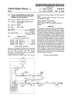
3.2 Calibration unit
The calibration unit illustrated in figure 21 performs the
wavelength calibration. A diffuse reflex from the laser is
transmitted into the unit where it is divided into two
parallel beams. One passes through a reference cell with
the gas that is to be measured and then to a detector (cell
detector). The other passes directly to a second detector
(reference detector). The output signals from the detectors
are sent to the system computer via the Control Unit in
the system cabinet. Looking at the quotient between the
pulses you can determine if the laser has drifted during a
measurement and it is possible to calculate the errors in
the measurement.
All interactions between the calibration program and the
unit are done through the Control Unit. All components in
the unit are powered from the Power Unit. For details see
appendix 1.
3.3 Laser system
When the project started the laser-system used in the
LIDAR-system was a tuneable dye laser pumped with a
Nd:YAG laser. This system was replaced with an GPOsystem, the MOP0-730 from Quanta ray. For details see
appendix 13.
Laser beam
Nd:YAG Laser
Optical component
that reflects the laser
beam
Calibration Unit
Detectors
Gas Cell
Mirror
Beamsplitter
Filter
Figure 21 Principal sketch on the calibration unit
15
Department of Atomic Physics, Lund Institute of Technology
4. System design
4. System design
4.1 Introduction
This section describes the components, electronics and
the communication in the calibration system. It also
describes how and why the parts have been designed or
selected.
4.2 General
To be able to choose components and design the
electronics one has to understand the purpose of the
measurement, what will be measured and what problems
arise when measuring.
4.2.1 Purpose
The purpose of the laser calibration system is to find the
deviation in frequency (wavelength) between the laser's
setting value and its real value.
This is achieved by comparing the spectrum of a known
and well-defined vapour in a gas cell with the results
from a measurement. I.e. measuring an absorption
spectrum in a region where the physical data is known for
the vapour.
When designing and selecting components for the
calibration system it is important to know what should be
achieved. At a first glance it may seem like it is the
energy of every pulse that is important to measure. But in
this case the absorption is relevant. Knowing the exact
energy of every pulse may give more information but it is
probably unnecessary to measure. Furthermore, it is not
the actual absorption (in exact figures) that is relevant. It
is finding the pattern of the absorption for the vapour.
4.2.2 Measuring conditions
The laser pulses that are measured contain typically some
10'3 Joule of energy. The length of the pulse is about 34ns and the laser repetition frequency is 20Hz (20 pulses
per second.) The wavelength range is between 250nm to
4800nm. The energy of the laser pulses fluctuates with
about 10%.
The pulses are transmitted into the calibration unit from a
reflection of the DIAL laser beam.
4.2.3 Problems
To be able to measure the exact appearance of the pulses
a fast detector is needed. To be able to hit the detector
when aligning the system, the active area must be at least
50mm2• These conditions contradict each other. The
bigger the detector becomes, the slower it gets.
The frequency range of operation is vast. It is a problem
to a find detector that is big enough and yet operates fast
enough in the whole range.
A fluctuating laser is a problem. If every laser pulse does
not have the same energy, it is not possible to know if a
change in measured energy is due to the laser or to a
change of absorption in the vapour.
Figure 22 Picture of the calibration unit in operation.
16
Department of Atomic Physics, Lund Institute of Technology
4. System design
The intensity of the pulse varies between different
experiments. The actual energy is dependent on how the
pulse was received (which reflection used) and how it is
transmitted to the calibration unit. The intensity can vary
several powers of ten.
Smooth operation of the unit is
Changing of the cells must be
with clips to which cells can be
be mounted with different sizes
so all kinds of cells can be used.
considered in the design.
simple. This is achieved
attached. These clips can
and at different distances
4.4 Detector
The laser pulse is extremely short. This makes it
extremely difficult to read the values directly from the
detectors with the computer AID-electronics.
The detector and its electronics are the most vital parts for
the calibration. These components determine the different
parameters needed in the program: maximal intensity,
minimum intensity and so on.
4.3 The calibration unit
Speed, size and operation-region are taken under
consideration when selecting detector.
All components that are chosen should manage the strain
in the lorry. Every thing has to be built robust. This can
be seen in figure 21 and figure 22.
In order to get the right amount of energy in the laser
pulses is must be possible to reduce the intensity. A
wheel with neutral density filters at the entry does this.
Splitting the beam into two beams reduces the problem of
a fluctuating laser. One beam is used as a reference.
When the energy of the pulses change it will change with
the same factor in both beams. By dividing the energy
value of the pulse travelling through the vapour by the
reference value the fluctuation is annihilated.
To come around the problem with the large frequency
interval a detector wheel is constructed. On this several
detectors can be installed.
The detector electronics must be constructed to measure
the value of the energy and then to hold the signal until
the computer program registers it.
Since everything will be controlled from a computer
program the unit also has to be completely automatic. For
this reason all components that need to be changeable are
mounted on wheels or cylinders that are controlled by
stepper motors.
To be able to measure on several gases during one
measurement a revolver wheel is constructed. In this
revolver up to 7 different cells can placed.
The parts in the calibration unit are constructed in blocks.
This is done to make it easy to rebuild or change the
components. The moving parts are mounted with the
stepper motor on a plate. This plate can easily be
removed from the unit for modification or replacement.
The modular construction also has the advantage that
parts not needed for the moment can be developed and
manufactured when needed.
4.4.1 Useable detectors
One detector that would serve the purpose is the SD29011-31-241 from Advanced Photonix Inc [14]. This diode
detector can measure between 300nm to llOOnm.
Other alternatives could be the S3590-05 or S3590-06
from Hamamatsu [15]. These detectors are fast and big
enough, 9x9mm. If the S3590-06 is chosen it could be
used between 190nm to 11 OOnm. One problem with this
detector is that it does not have any protection window.
This would make it sensitive to humidity and human
touch. To get around this problem a quarts window with
good quality could be mounted in front of the detector.
One detector that would work is the 2-Watt Broadband
Power/Energy Meter from Melles Griot [ 16]. This
detector can measure from 200nm to 20J..tm, i.e. more
than enough. It works with frequencies up to 60Hz. The
problem with this detector is that it can not be connected
directly to the computer. It comes with a control unit.
Another problem is that it needs rather high pulse energy.
High pulse energies can cause stimulated emission in the
gas cell that disturbs the measurement.
The detector from the old calibration unit is the S13371010BQ from HAMAMATSU, for detailed data see
appendix 17. This detector is too slow to measure the
actual pulse. When looking at the output from the
detector in an oscilloscope it is found that the length of
the pulse is some J..lS but it is know that the laser pulse is
some ns long. But since it is the absorption and not the
actual energy in the pulses that is of interest, it is possible
to use this detector. In an experiment that was performed
it was shown that the two detectors are linear towards
absorption.
17
Department of Atomic Physics, Lund Institute of Technology
4. System design
4.4.2 The chosen detector
The old detectors were chosen since they fourfold the
necessary conditions.
To be able to understand why this slow working detector
works one has to understand how a photodiode works.
Basic photodiode theory
A photodiode is a solid state device that converts light
into electric current. It normally consists of doped silicon
that forms a so called p-njunction, see figure 23.
SiO, (thermally grown)
AR Coating ~
..·.
.
P+
F
Front Contact
A~tive A;~~~,-
,Depl.:~ti91l8eglon
<. /
--·
i
'
p-n Junction Edge
n-Type Silicon
n+Back Diffusion ~------ ·--"
Back Metalization
the minority carriers to reach the region before they are
recombined.
How the old detector works
The old detector does not measure the actual laser pulse.
The fast pulse injects electrons and holes into the
depletion region. These charged carriers drift towards the
depletion region. If the carriers reach the region before
they recombine the charge can be measured. This process
in the detector is much slower than the actual laser pulse
but if the number of carriers that is measured is
proportional to the energy in the laser pulse, there is no
problem using these detectors.
4.5 Digitizer trigger delay
The laser triggers the synchronisation of the system. The
laser sends out a trigger pulse, see figure 24. This pulse is
transmitted to the control unit where a new pulse is
generated by the digitizer trigger delay, see appendix 12.
This new trigger pulse is then used to synchronise the
electronics.
Figure 23 Basic configuration ofa photodiode [ 17]
v
15
The n-type region is created when impurities, i.e. other
atoms, with extra electrons are defused into the silicon.
These atoms are called donors since they "give" away
their extra electron. The p-type silicon is created in the
same way but the silicon is doped with acceptors, or
holes. These atoms accept electrons.
When the two regions are in contact the electrons in the
n-doped region and the holes in the p-doped region feel a
lower potential on the opposite side of the edge. This
potential difference makes the electrons and holes flow
across the p-n junction. This charge movement
establishes an electric field that works against the
movement. After some time equilibrium is established
and a depletion region has been created between the two
regions.
When photons fall on the device, they are absorbed and
electron-hole pairs are created. The electron hole pairs
drift apart, and when the minority carriers reach the
junction edge, they are swept across by the electric field.
If the two sides are electrically connected, an external
current flows through the connection. The photodiode
behaves as a current source when illuminated.
If the created minority carriers of that region recombine
before reaching the junction field, the carriers are lost and
no external current flows. An external voltage is applied
to the photo diode to increase the sensibility. This will
increase the depletion region i.e. make it more likely for
10
Trigger pulse from the laser
To the controle unit
5
ms
2
v
3
4
Trigger pulse from the controle unit
To the controle detector electronics
Signal from the detector
J.lS
Figure 24 The trigger pulses
18
Department of Atomic Physics, Lund Institute of Technology
4. System design
4.6 Detector electronics
The detector electronics will amplify the signal from the
detectors, integrate the signal and hold the value until the
computer reads it. All this has to be done in
synchronisation with the laser.
Details about the detector electronic are found in
appendix 11.
4.6.1 Basic design
In the lorry the voltage is 12V. This voltage is
transformed on the circuit board to 5V that is used as
input by the components, see appendix 11.
The pulse from the detector has to be amplified. A
preamplifier does this, see figure 25.
The signal from the preamplifier is then integrated with a
standard integrator, see figure 26.
After the integrator the signal is again amplified by a
follower, see figure 27.
The mechanism to hold the signal until the computer can
read it is constructed by using the fact that there is a large
difference in energy between the laser pulse and the
background. The signal from the detector is almost zero
when there is no laser intensity.
The integrator will accumulate the signal from the time
when the trigger is received until the value can be read by
the computer, but since there is no output after the laser
pulse the circuit will "hold" the signal even though it is
integrated.
To reset the integrator a short circuit is put over the
integrating capacitor. This short-circuit is kept until the
low flank of the trigger signal is received, see figure 24.
The detector pulse is then integrated until the capacitor is
short-circuit again, see figure 28.
Short-circuit
pulse
74121
Trigger In
Figure 28 Short-circuit part.
Amplification= (R1 +R2)/R2
When the low flank is received in the trigger in, the
short-circuit is released and the capacitor can
integrate the signal.
The integration time= 0, 7*RC
Figure 25 Preamplifier.
4.6.2 Trimming the parameters
c
Output = -1/(RC)
Trimming the circuit parameters is done on the integrator
circuit. If one part is badly adjusted other parts can not
correct this error.
The dynamics in the system must be as big as possible at
the same time as no part should be saturated.
.fu dt
Figure 26 Integrator.
To be able to determine the values of the resistors and
capacitors an experiment was conducted on the detectors
with electronics, see appendix 18. This experiment
showed problems with offset and badly balanced
electronics. This is illustrated in figure 29. If the detector
electronics are not balanced the output value can increase
or decrease over time. It takes some time until the
computer reads out the value. During this time the value
can change, see figure 29. This will lead to errors in the
measurements.
Output= Rl/R2
Figure 27 Follower.
19
Department of Atomic Physics, Lund Institute of Technology
4. System design
...
3
1
2
/
..
...
(
.
flow of clean air. If this was to be used then it had to be
enclosed .
,:
... .. . . .
...
)
A decision was taken that it would take too long to make
a changeable beam splitter device. Therefore only the
original beam splitter was installed.
4.8 Neutral density filters
\
J.LS
Figure 29 Problem with offset.
4. 7 Beam splitter
The beam splitter divides the light from the laser to the
detectors. This is done in order to use one detector as
reference. In this way compensations for the fluctuations
in the laser energy can be made.
The demands on the beam splitter are
• A 50150 distribution, but if slightly more of the
intensity travels through the gas cell it would be good
since the gas will absorb some light.
• Operate in the entire specified wavelength region with
the same splitting ration.
A problem when splitting laser beams is that the laserlight is polarised. Beam splitters often split the light
differently in the p- and s-plane. The pulses that will be
used are derived from a reflection from some optical
component in the beam path of the OPO-system. Which
component used depends on the experiment the OPOsystem is used for, i.e. the direction of the polarisation
will change between experiments. For this reason the
beam splitter must have the same division in both
directions.
To be able to cover the whole range a number of beamsplitters need to be installed. A normal beam splitter from
manufacturers has its operation region within a couple of
hundred nanometers. The problem is to get a reasonable
number of beam splitters.
The problem can be solved with the pellice beam splitter
nr 03 BPL 001 /04 from Melles Griot [16]. This beam
splitter has a 40/40 splitting between 400 to 1060nm.
Above this region normal quartz can operate, and below
the original beam splitter works fine. In other words three
beam splitters would cover the whole region.
The filter wheel is used to adjust the intensity of the laser
light. The problem is that the laser produces light that is
much to strong for the unit. Even a reflection from the
laser beam has to high intensity. The unit must therefore
be able to reduce the intensity of the light several powers
often.
During the experiment described in appendix 18 the
optical density of each different filter was found. The
filter wheel has 10 positions. This allows a maximum
decrease of intensity down to 4% (9 positions are used for
filters and one is blocked to protect the unit). The result is
shown in Table 1. Due to economical reasons old filters
are used. The filter set-up used is described in table 2
Position
0
1
2
3
4
5
6
7
8
9
Transmittance[%]
0
4
6
8
10
20
40
60
80
100
RoundedOD
Blocked
1,4
1,2
1,1
1,0
0,7
0,4
0,2
0,1
0,0
Table 1 The best choice of filters
experiment in appendix 18.
Position
0
1
2
3
4
5
6
7
8
9
according to
Optical Density
Blocked
Blocked
3,0
2,0
1,0
0,7
0,4
0,2
0,1
0,0
Table 2 The optical density of the filters that are used in
the unit.
The problem with this beam splitter is that it is sensitive.
It may not be touched and only be cleaned with a gentle
20
Department of Atomic Physics, Lund Institute of Technology
4. System design
4.9 Stepper motor
The chosen stepper motor is the two phase KP56LM2502 from ELFA [18]. This motor can operate as a
unipolar as well as a bipolar motor. The bipolar
configuration is chosen, see appendix 14.
4.10 Stepper motor electronics
To power and control the operation of the stepper motor
the GS-D200S driver from ELF A is used [ 19], see
appendix 15. To be able to configure and use the module
it is mounted on a circuit card as shown in appendix 7
The configuration is as follows (for pin description see
appendix 15)
• Pin 4 (Half/Full) is connected to earth.
This means that the full step mode is selected. Half
step mode makes the drive module step the motor
with half steps i.e. the double number of steps is
needed for the motor to make one revolution. The
stepper motor has 200 steps/revolution. That is
enough for the components in the calibration unit.
• Pin 9 OosET) is connected to Pin 1 (GND 1) via a
300Q resistor.
This is done to lower the current to the stepper motor
in order to prevent over heating. The resistance can
be calculated from R=I/(3.03-1.43xi)kQ where I is
the current. The operation of the motor does not need
high hold torque. Because of this the lowest currency
(=0.5A) is chosen. This gives a resistance of0.22kQ.
The resistance is set to R=300Q which gives a
current 1=0.64A. This is below the suggested value
when driving the motor m bipolar mode.
See appendix 14.
• Pin 1, 4, 6, 7, 9, 12, 13, 14, 15, 16, 17 and 18 are
connected to cable connectors.
• Pin 2, 3, 5, 8, 10 and 11 are not used.
The four stepper motor-boards are mounted in the powerunit. Here cables are connected from the cable connector
on the circuit card to other cable connectors in the unit.
See appendix 6. This is done for easier handling.
The wheels in the unit are added with a peg or a hole that
will block or let the light pass when the start position is
found.
4.12 Power unit
The power unit consists of several components to control
and power the different parts of the LIDAR-system see
figure 30. It is connected to the control unit as well as to
the calibration unit. For additional information about the
components in the unit see [1].
For the calibration system the unit has been fitted with:
• Stepper motor board (motor 5 to 8) to steer the motors
in the calibration unit.
• Connector to the control unit for cables related to the
calibration system.
• Connector to the calibration unit.
• Additional power supply to the stepper motors.
4.13 Control unit
From the control unit the different components of the
LIDAR-system are controlled. In this unit there are
connection boards for wiring to the AT-MI0-16 and the
PC-TI0-10 in the system computer. See figure 31. For
additional information about the components in the unit
see [1].
For the calibration system the unit had to be added with:
• Connector to the power unit for the cables related to
the calibration system.
• BNC connectors from the detectors in the calibration
unit.
4.14 System computer
A PC is used to run the calibration system. This computer
is equipped with several PC-cards to be able to send and
acquire data form the LIDAR-system. The PC-cards used
to communicate with the calibration system are the PCMI0-16 and the PC-TI0-1 0 from National Instruments
[7].
4.11 Position detector electronics
Finding the exact position of the components is extremely
important. If the positions are not known, it would not be
possible to select detector, gas cell or neutral density filter
i.e. it would be impossible to use the unit.
The position detector is used to find the locations of the
components. The circuit drawing is found in appendix 10.
The operation is simple. If the light from the diode hits
the detector there will be +5V on the OUT and OV on
"inverse OUT". If the detector light is blocked the
opposite will occur, OV on OUT and +5V on "inverse
OUT"
21
Department of Atomic Physics, Lund Institute of Technology
4. System design
4.14.1 AT-MI0-161/0 PC-Card
4.14.2 PC-TI0-10 PC-Card
The MI0-161/0 PC-card consists of 12-bits ADC with 16
analogue inputs, two 12-bits DAC's with voltage output
and eight lines of TTL compatible digital 1/0 interface.
This card is used to acquire the analogue signals from the
calibration system i.e. the signal from the detectors.
The PC-TI0-10 PC-card is a timing and digital 1/0
interface. It consists of sixteen TTL compatible digital
1/0 lines, ten counters and has two edge-sensitive
interrupt inputs with programmable edge selection. This
card is used for the TTL input and out to the calibration
system.
The PC-card is connected to the control unit with a flatcable. The cable is connected to a 50-pins connector
board. For details of the wiring see appendix 1 The
Wiring of the system.
0
s.sTW lAS"R
""""' """"'
[][OJ
-D -rn~~~Y~@
';"'0
0
The PC-card is connected to a 50-pin connector board in
the control unit. For details of the wiring see appendix 1
The Wiring of the system.
0
0
0
@®~
Of •
@
R:Ma0
CUT.lin
""""'50
[]
0
0
RortPcnel
OJratflrl'Pilia-
,-----
IL
I! !
~J J
j
~c
~
H91V<fuge
R:Ma-S.Wy
~
~
an
~~~~
'--
I
'-----
I
D..el celay
Olnnector l3csti
D024VO
JI~~ 00! 00
.~
j-
_;re
~I
R=layos
I
II~ I
O;taia-
FC-11010
Sgra R=lay
DD~ ~D_[J
-
M0161/0
®
®
®
(!)
J4..5J5J7
RB-Pcnel
CK:l.,J\O(J1)
t
CXJ.M:N® ® ® ®
GR::A...K>(J1)
~
GJ9
J:lD
J19 J18J11 J10
FOIIffi'J2l
~
®.e
[]0241/0(J12)
S'ISTEM(J4)0 J1
MQ.16110(J13)
~
l.ASER(J3)
FC110-10(J14)
J16
~
\l\hjili1
J15
®..6
®..6
[OJ
~
,<>rge
"""""'
[)J
'
""""l.nt
Figure 30 Overview of the control nit
Figure 31 Overview of the power unit.
22
Department of Atomic Physics, Lund Institute of Technology
5. User manual
5 User manual
5.1 Introduction
This manual describes the calibration program from a
user perspective.
peak data for the cell is displayed. The selected cell will
be the one used if a calibration is started.
Current cell selection box
This box shows the cell that is currently ready for
calibration. With this control it is possible to change the
cell that the calibration shall be performed for, see
figure 33.
The calibration program consists of two parts,
configuration and calibration. The calibration part is
called from other programs in the LIDAR system. The
actual calibration is done automatically even though the
calibration properties are retrieved from the configuration
part.
If the cell is changed the new cell will be rotated to the
calibration position in the unit and the default data for the
new cell will be displayed.
The only user interactions in the calibration part are
dialogue boxes displayed when errors or problems in the
calibration are detected. For this reason only the
configuration part is described in this manual.
"Change" button
This button is used when the configuration in the
calibration unit is to be changed. When pressed the
Change in calibration unit front panel will be displayed.
For a description of the calibration part and for technical
details please refer to the 6 Programmer's Guide.
5.2 Configuration part
In the configuration part of the program, the calibration
unit is set-up, the cells with vapour are defined and the
calibration method is defined. The settings from this part
are used when the actual calibration is performed.
J
. ·. ··•··· 'J.
~--~~~------~~~~~.~.~·~
·Current Cell:
Wavelength on:
The configuration of the unit is done from three main
windows:
•
Current calibration settings. Used to show the
current settings of the calibration unit. From this
module the data to the calibration part is passed on.
From this panel it is possible to display the "Change
in calibration unit" front panel.
•
Change in calibration unit. This front panel is used
to configure the calibration unit i.e. change the cells
in the unit. From this panel it is possible to display
the "change calibration data" front panel.
• Change calibration data. This module is used to
configure the calibration data for a cell.
In the calibration system many cells can be configured.
For each of these cells many calibration regions can be
defined i.e. data used when calibrating with that cell.
These regions are called Peak or Peak Data. For each cell
one peak is defined as the default peak. The data for this
default peak are used by the system when calibrating
using the cell. This means that if non-default peak (data)
shall be used for calibration then this peak has to be
changed to the default peak for the cell.
5.2.1 Current calibration settings
This module displays the current settings m the
calibration unit, see figure 32.
·wavelength off:
J
Figure 32 Front panel of the Current calibration
setting.
J
Current Cell: ·
Wavelength on:
Wavelength pff:
Calibration mode:
Detector:
Bearn splitter:
J
Figure 33 Front panel when changing the cell.
From this screen it is possible to select one cell. When a
cell is selected the name of the cell along with the default
23
Department of Atomic Physics, Lund Institute of Technology
5. User manual
5.2.2 Change in calibration unit
This module makes it possible to change the cells in the
calibration unit, se figure 34.
Calibration Cell selection box
Displays all the calibration cells that are defined in the
system.
This button is used if a defined cell shall be erased from
the system. To delete the cell, highlight it in the
Calibration Cell selection box and then press the "Delete
data" button. A warning message box, in which the action
has to be confirmed, is displayed before the cell is
removed.
Cell in Revolver selection box
Displays all the cells that are present in the calibration
unit.
Calibration Peak selection box
Displays all calibration peaks for the cell that
highlighted in the Cell in Revolver selection box.
,.)
IS
"Change Data" button
This button is used if the calibration data for a defined
cell is to be changed. To change the data the cell has to be
highlighted in the Calibration Cell selection box. When
the button is pressed the program will open the front
panel for the Change Calibration Data.
"New Data" button
This button is used when a new calibration cell shall be
added to the system. When pressed a dialogue box is
displayed, in which the new name of the cell shall be
typed, see figure 35. After the name is entered the
program will open the front panel for the Change
Calibration Data, see below.
"Delete" button
Figure 35 Front panel of "New Spiece Name. vi".
This VI is used when a new cell shall be added to the
system.
J
Cell in Revolver
Calibration Cell
II
N02
502
HG nr 1
HG nr 2
.. <- Remove <-
.. ->Change->
J
J
t·J02
·u
448, ZOO
HG nr 1
Defult
Change Data
New Data
J
Delete
J
J
J
Re.set UNIT
J
Figure 34 The front panel for Change in calibration unit. The configuration of the calibration unit is executed from
this VI.
24
Department of Atomic Physics, Lund Institute of Technology
5. User manual
"Remove" button
This button is used when a cell shall be removed from the
calibration unit.
The program checks if there is a cell present in the unit. If
not, a warning message is displayed.
The revolver will then be moved to make it possible to
remove the cell. A dialogue box is displayed, see
figure 36, in which the action shall be confirmed.
Confirm when }lou have
removed the cell
at position: 0
,. OK.
j
i
Cancel
J
Figure 36 Confirmation dialogue box.
"Change" button
This button is used when a cell shall be added to the unit.
The cell is highlighted in the Calibration Cell selection
box. The position where the cell shall be inserted in the
unit has to be highlighted in the Cell in Revolver
selection box.
It is possible to change a cell even if the position is
occupied. It is not possible to have the same cell in two
positions in the unit at the same time.
When the action is performed the program checks if the
cell is present in the unit. A warning message is displayed
if the cell has already been added. Then the revolver is
positioned so it is possible to add/change the cell. A
dialogue box is displayed in which the action shall be
confirmed, see figure 36.
"Default" button
This button changes the default peak for the cell
highlighted in the Cell in Revolver selection box. The
peak that becomes default is the one that is highlighted in
the Calibration Peak selection box.
"Reset UNIT" button
This button shall be used when the set-up in the program
does not correspond to the actual configuration in the
unit. This action will NOT reset the cells and data
defined in the system.
"OK" button
Saves all data and exits the panel. The program will
returns to the Current calibration settings front panel.
25
Department of Atomic Physics, Lund Institute of Technology
5. User manual
5.2.3 Change calibration data
This module makes it possible to change the data for a
cell, see figure 37. All data needed for the calibration is
configured in the display. The data that is used for
calibration depends on the calibration mode used. The
data for a highlighted calibration peak is displayed in the
left field.
"Calibration Data" box
In this box the calibration values for a specific region are
changed and edited.
"Calibration Peak" selection box
Displays all the calibration peaks for the cell.
"Add Data" button
When this button is pressed the data that has been entered
in the Calibration Data box is checked. If the data is
correct (within thresholds) it is added to the cell.
"Copy" button
When pressed the data for the highlighted peak is copied
to the edit field.
"Default" button
Changes the default peak to the highlighted. The default
peak is displayed with two stars in front of the data.
"Delete Data" button
Deletes the peak that is highlighted in Calibration Peak
selection box. If the peak is the default one, then default
setting will change to the peak that is first in the list.
"OK" button
Exits the panel and returns to Change in calibration unit
front panel.
"Change Data" button
When pressed the data in the edit field is checked. If the
data is correct the data for the highlighted peak is
changed.
CellNt~me: .,._N_D_2_ _ _ _ _ _ ___,
Calibration Peak
J
Calibration Data
Wt~velengtfl On:
<
·,:::
,·'
Wt~velengtfl Off"
~1448.1 0000
~1447.50000
Wav On
· nrav Off.
447,500;
44~r.zoo
[nmj
[nmj
[nmj
[nmj
[nm/sttfp]
fll
~eS:ri'x~d.
447,000
. Stt~/1 OFSct~n:
~1448.50000
·End OFSct~n:
31447.70000
· Step lntewt~fL·
310.05000
.. DilL Absorption.: ~lo.ooooo
Ct~h"brt~lion Mode: ·~~lc::al::ib=ra=tio=n=1=-~~
.) ""''*_A...d_d_D_at_a_·_...)
,_Change Data
JJ
,_
.,_
,_
Copy
Default
Delete Data
J
J
Figure 37 Front panel of "New Spiece Data. vi". In this VI the data for a calibrating cell can be changed
26
Department of Atomic Physics, Lund Institute of Technology
6. Programmer's guide
6 Programmer's guide
6.1 Introduction
This guide describes the concepts of the calibration
program. It is intended for programmers and persons who
want to change or add functionality to the program.
The guide has three sections. The first section (6.2)
describes the basic concepts and the main parts of the
program. The second (6.3) describes the program in
further detail and how to add functionality. The third
section is an overview of the Virtual Instruments (VIs)
and the main data clusters in the program. This section is
found in appendix 19 VI and Cluster description.
6.2 Basic concepts
This section describes the basic design pattern of the
program. It also gives an overview of the calibration
program.
6.2.1 Introduction
The calibration program consists of two parts. One part
handles the configuration of the unit and sets the current
data that are necessary to calibrate. The second part
handles the calibration. These two parts are separated
although the calibration part uses the data set by the
configuration part.
Since the calibration program is one part of the total
LIDAR-system developed by the LIDAR-group, there are
some basic rules that must be followed.
6.2.2 Basic design
In this section the basics of the program are explained.
These things are:
• Stopping of the program. There must be a way to stop
the program at any given time.
• Screens for input of data.
• How to control the sequence of execution.
• How data is passed to the different modules.
• The main data clusters in the program.
• Storage of data from the calibration program.
• Parameters in the program.
6.2.2.1 Stopping the program
To be able to stop the program at any time two global
Boolean have been implemented. These are "Change
activity" and "Run". If the system has to change activity
the "Change activity" variable is set to TRUE. All
modules in the LIDAR system shall then stop to make the
action possible. In the same way the "Run" variable is
set to FALSE when the system shall be shut down.
These two variables are never set in the calibration
program, but they are checked to determine if the
program shall continue execution or not. Two VIs are
implemented to perform the check. These are
"ContinueExecErrorCheck" and
"ContinueExecNoErrorCheck". The difference between
these is that the first one also checks if there are any
errors in the Info cluster. For further information, see
appendix 19. The first thing done when a VI is called is to
check if every thing is OK. This is done as in figure 38.
In "For" and "While" loops the ContinueExecNoErrorCheck is used, see figure 39.
6.2.2.2 Input screens
The performance of the input screen is achieved as seen
in figure 40.
First the VI checks if it shall execute or not. Then the VI
is initialised. After this two loops are started. The lower
loop is responsible for collecting the user input, i.e. which
buttons are pressed on the front panel. The upper is
responsible for performing the tasks related to the button
pushed.
An occurrence object achieves the synchronisation of the
loops. The upper loop enters the default case where it
waits for occurrence from the lower loop. Every 200ms
the lower loop checks if any button is pressed. If a button
has been pressed the variable execution frame is set to
the case number that shall be executed by the upper loop,
and the occurrence is generated. After this the lower loop
waits for the occurrence from the upper loop. The upper
loop performs its tasks and when ready it returns to the
default case. Here it generates the occurrence, so the
IActivities are performed here
Figure 38 Before executing the code the status is
with ContinueExecErrorCheck.
m
!Standard while loopl
con t
r.::=:J
EXEC?··~
No Err
Figure 39 for every loop the status is checked with
ContinueExecNoErrorCheck.
27
Department of Atomic Physics, Lund Institute of Technology
6. Programmer's guide
True
0. Default
~:=:;=::_-W~-fill-...m
Waits here until a button is pressed.
Then reads Execution frame and goes
to the frame with that number.
Figure 40 Standard code for an input screen.
lower loop can start again, and then it once more waits for
the lower loop.
6.2.2.3 Synchronisation in the program.
The execution sequence in the program is achieved by the
data flow of three clusters. These are:
• The "Info" cluster.
• The "File Types" cluster.
• The "Calib" cluster.
These clusters carry the data within the system. The
"Info" and "File Types" cluster are general clusters
containing data of the total LIDAR-system while the
"Calib" cluster is used only in the calibration program.
6.2.2.4 The "Info" cluster
In the calibration program all the VIs have the "Info"
cluster as input. This cluster is the main object for the
synchronisation. If an error occurs the error number is
saved in this object. See figure 41.
This cluster carries all the current settings and data of the
calibration program. That is the current position of the
revolver, position of the detector etc. It also carries the
data used by the calibration part to make the calibration.
The different parameters are explained in 6.2.2. 7 The
data structure.
Speed(Hll
·.
I ~.;._lo.,.,..........._,_...;....,.....J
Current Rev Posl
Peak DataL
~lo
..
lo
I
·
Current Detector Posl
lo
I
. ·
Current SplitterPosj
lo I
·
Current Filter Posl·
lo I
·
Calib Cell Rev Posj
lo
I
Calib Delector Posl
lo
I..
lo
I
Calib Splitter Posj
Test Model
D
.·
.\\fav~l~ngthDNl
0,00000· . :
W~v~~~~gth oi=FI
§goqoo_..
:>.·
StartOfScanP ··
o.oooocC ; •:_ ·
o,ooooo''
Ste~· .· .
EndOfScanL
0,00000 .
.Diff Abst_·
.Q,OOOOE~O·•····
·Calib S~Jector[
0·
Figure 41 The parameters used by the calibration
program in the Info cluster.
28
Department of Atomic Physics, Lund Institute of Technology
6. Programmer's guide
6.2.2.5 The "File Types" cluster
This cluster contains the data needed when making file
transactions. See figure 42. This cluster is only passed on
to VIs that need to save or retrieve data from the
calibration file. More information about saving the
calibration data is found in section 6.2.2.8 Data storage.
It is important to see the cells, detectors and beam
splitters as physical objects. Each cell that is defined in
the system shall have a physical cell. For this cell many
different calibration regions (peaks) can be defined.
The different parameters are explained in 6.2.2.7 The
data structure.
Parameters used by the calibration program
Calib Data File Path
The file path to the calibration data file. The path
includes the file name.
Cell
The data format that is saved to the file. The
information is in the same format as for the
Calib cluster, see 6.2.2. 7 The data structure.
Cel/Refnum
A position reference used by LabVIEW when
reading and writing to the file.
6.2.2.6 The "Calib" cluster
6.2.2.7 The data structure
The structure of the data in the program is shown in
figure 44. In this figure the dependency between the
clusters is shown. For detailed information about the
different elements in the clusters see appendix 19 VI and
Cluster description.
6.2.2.8 Data storage
Three things are important when designing data storage:
1. The configuration should not be lost when the
program is terminated
2. Dynamic data shall be easy to change.
3. All dynamic data are retrieved at a restart.
It contains all the data that is necessary to configure the
calibration unit, i.e. the data for every cell of vapour, the
calibration peaks for the cell, the detector and splitter
settings. See figure 43.
When looking at these three criteria it is found that the
dynamic data are the cell data with all the peaks (the
calibration data) together with which cells are present in
the revolver. When restarting the program these data need
to be retrieved.
The position of a cell in the revolver is stored in the
File Type:s inl
Calib Data File Pathl
'
CeiiRefliuml
Info File Pathl
Measurement Specification File Pathl
I . . . :. '_ __;_,_.~I '
-
I
··9ll!J
Peaks For Celli
Pos in Revolver!
~
Defult datal
~
Last Datal
~··
Po:s in Revolver!
~
·Defult datal
~
Last Datal
~
~~ i)
.
. -
l.
~~-~ .....·~·.....~...............:,;,,.,;.:.-....'..,;.l
Measurement Info Refnuml
:: ·: .
'Measurement Info
II Soeciesl.
Figure 42 The parameters used by the calibration unit in the File Types cluster.
29
Department of Atomic Physics, Lund Institute of Technology
6. Programmer's guide
"Cell" cluster in the array of "Cells" in the "Calib"
cluster, see figure 44. This "Cell" cluster is saved to disk.
The data for the detectors and beam splitters are static
data i.e. the data does not change often. For this reason
the data are not stored on disk, but are instead hard coded
in the initialising section of the program.
6.2.2.9 Parameters in the program
To be able to run the program some parameters have to
be defined. For detailed information on the parameters
that can be set see appendix 19 VI and Cluster
description.
The configuration of the parameters has to be done for:
•
Initialising of the unit.
Configured in VI: /nit Calibration Unit
•
Checking calibration data.
Configured in VI: Check Peak Data
•
Finding motor position 0.
Configured in VI: Find Motor Pos 0
•
Moving a motor.
Configured in VI: Rotate Selected Motor To
•
Changing cell in the revolver.
Configuration in VI: Change In Revolver
•
Finding neutral density filter.
•
Configured in VI: Select Demp Automaticaly 2
Calibrating
Configured in VIs:
Calibration Method 0
Calibration Method 1
Calibration Method 2
•
Indexing of the motors.
The addressing of motors in the program is done by
an index. This index is NOT the same as the motor
number in the calibration unit. The difference has
evolved since there are more motors in the LIDARsystem. The numbering of the motors in the program
is found in table 3 below.
Index
0
1
2
3
Motor
5
6
7
8
Description
The detector motor.
The revolver motor.
The filter motor.
The beam splitter motor. This
motor is not implemented in the
calibration unit.
Table 3 The numbering of the motors in the
program.
Calib in
Last Celli
~
Last Delector!
~
Calib cluster-
Last Splitterl
~
n~
!.·'; !. '~,:,:.:-~_i_i.t.:.J~.~-~.i.~-~.:-~.:~:~ 1
'=·,!,:
...
n:
1! i
~ !!
...................:::·::::··::·....·.. :·::::.. ::::::.: ............ ::·:·:·:-:-_1__ :
Last Cell
Last Detector
Last Splitter
Splitters (Array)
Name
Wavelength ON
Wavelength OFF
Detectors (Array)
Name
Wavelength ON
Wavelength OFF
Cells (Array)
Name
Pos in Revolver
Defult data
Last Data
Peaks For Cell (Array)
File Types cluste
Wavelength ON
Wavelength OFF
Start Of Scan
End Of Scan
Step
Diff Abs
Calib Selector
Current Rev Pos
Current Detector Pos
Current Splitter Pos
Current Filter Pos
Calib Cell Rev Pos
Calib Detector Pos
Calib Splitter Pos
Test Mode
Figure 43 The Calib cluster
Figure 44 The three clusters and the elements that is
defined for the calibration program.
30
Department of Atomic Physics, Lund Institute of Technology
6. Programmer's guide
6.3 Calibration program
This section describes concepts of the program, i.e. where
different data can be found and the logic behind.
•
•
The main components of the program are described with
a flow chart. For detailed information of the program
please see the code.
•
•
6.3.1 Basic concepts
The basic concepts of the calibration unit and program
are as follows:
• Revolver for 7 cells.
• Neutral density filter wheel with 10 positions.
• Detector wheel with 2 positions.
• The unit is prepared for adding a variable beam
splitter component. All indexing in the program
starts with zero. This means that the first position of
the neutral density filters, cell positions, detector
•
•
•
A(s:)
~y
Beginning and end point of the program sequence.
Prosess I Action
A process or action performed by the program.
•
•
•
•
positions, and so on is 0.
The program can be configured with data for many
cells.
For every cell that is defined there shall exist a real
cell.
For each cell many different calibration wavelengths
can be defined.
For each of the wavelength a specific calibration
method can be selected.
No detector shall be placed at position zero. In other
words the first real detector is found at position 1.
This is done to protect the detectors. The program
will always set the detectors at position 0 (blocked)
except when collecting data during a calibration.
The filter wheel will always move towards a darker
filter except when trying to find the optimal filter
during calibration. The program starts with the
darkest filter.
Detector 1 is the measuring detector i.e. the detector
that collects the signal from the laser beam that
passes through the calibration cell.
Detector 2 is the reference detector.
The current positions of the detector wheel, the
revolver wheel, the filter wheel and the beam splitter
are always stored in the Info cluster.
One cell at a time can be selected for calibration. The
data needed to calibrate is stored in the Info cluster.
All data configured in the program is stored in a
configuration file. This file includes information
about which cells that are present in the unit.
Manual operation that can be performed by the user. A
typical example can be when the user presses a key.
~
Message or screen that is displayed.
Predefined
process
Calibrate The
Laser
Process containing several actions. An example is
another main VI.
~
Decision. Typically an if statement.
Case 1
Case2
Case sequence.
Figure 45 The components used in the flow chart.
Figure 46 Main sequence of the calibration program.
31
Department of Atomic Physics, Lund Institute of Technology
6. Programmer's guide
6.3.2 Flow charts of main components
This section describes the main program.
The flow chart objects that are used are mainly standard
objects. The objects used are displayed in figure 45.
6.3.2.1 Main flow chart
The main components of the program are displayed in
figure 46. The figure shows the two parts of the
calibration program, the configuration part and the
calibration part. The main LIDAR program shall, during
normal operation, call the configuration part.
The calibration part is also called from the main
application. This can be done whenever it is necessary.
Since this part is a separate component other interfaces
can be constructed to use it.
6.3.2.2 Current calibration settings
This VI is the entry point to the configuration section of
the calibration program. The VIs front panel is the user
interface for selecting which cell shall be used when
calibrating the laser. See picture 47.
The name of the VI is: Cell Selection.
This VI shall be called with a regular interval from the
main program.
The first time the VI is called a parameter shall be set so
the program knows it shall initialise the calibration unit.
This parameter can be set every time a recalibration is
wanted.
When calling the VI the program checks if it shall
initialise the unit or not. When initialising the unit the
program will set all motors in the unit to their starting
positions. Then the saved data is fetched from a
configuration file. The front panel screen is updated, and
then the VI returns to the main program.
If the VI is called without the initialising parameter set it
will check if anything has changed from the "previous
visit". The things that can have changed are:
• The change button has been pressed. The VI will
then call the VI for configuration of the calibration
unit, see section 6.3.2.3.
• A new cell for calibration might have been selected.
In both cases the display will be updated and the
configuration data will be stored in the Info cluster.
6.3.2.3 Configuration of the calibration unit
This is the user interface for configuring the calibration
unit. From this screen cells can be added and removed
and calibration data can be changed. See picture 48.
Configuration Of
The Unit VI
Initialisation of the
VI
Print of data to
screen
8
Figure 47 Flow chart for Current Calibration Settings
32
Department of Atomic Physics, Lund Institute of Technology
6. Programmer's guide
The name of the VI is: Configuration Of the Unit. This
VI is called from Cell Selection, see section 6.3.2.2.
When called, the front panel of the VI is displayed. This
screen will be open until the OK button is pressed or until
an error occurs.
When changing in the unit, the current positions of the
motors are always stored in the Info cluster.
All the cell data that are changed or added is stored in the
Calib Cluster. This is done instantly when the change is
made. The screen is also updated when changes are made.
In this way the screen and the Calib cluster are always
mirrors of each other. Because of this relation, the index
of the highlighted field is used directly when operations
Figure 48 Flowchart for the configuration of the unit.
33
Department of Atomic Physics, Lund Institute of Technology
6. Programmer's guide
are carried out on the cluster.
Example: If the peak data for an existing cell shall be
changed the user will first highlight the cell on the screen
and then press the button to change the data. Since the
screen and cluster are "reflected images" of each other,
the program now know that the index of the highlighted
field on the screen is the same as the index for that cell in
the array "cells" in the Calib cluster. When exiting the
Configuration Of the Unit, the data of the Calib cluster
are stored to the calibration file.
6.3.2.4 Edit peak data for cell
This is the user interface changing the peak data for one
cell, See picture 49.
The name of the VI is: "Edit Peak Data For Cell". The
VI is called from "Configuration Of the Unit", see
section 6.3.2.3.
The VI is called with an index parameter. This index is
the position of the cell in the array "cells" in the "Calib"
cluster. All operations will be performed on this cell only.
6.3.2.5 Calibrating the laser
This VI is the entry point to the calibration section of the
calibration program. The VI is called from the main
application and has no direct interaction with the
configuration part of the calibration program. But when
the VI is called the calibration parameters in the "Info"
cluster must be set. It is in this VI all the different
calibration methods are called, see figure 50.
To move the OPO-laser to a specific wavelength the
program uses components developed by Fredrik Nordin
[20]. The calibration program calls these VIs with the
wavelength the laser shall move to.
The name of the VI is: Calibrate The Laser.
Input parameter: "Info" cluster. The calibration
parameters must be set in the cluster, when called.
Output parameters:
I. "OK out". Tells if the calibration was successful or
not.
Print of data to
screen
Display Error
message
Add Data
pressed
Add the new data
Change Data
pressed
Copy Data
pressed
Change the default
peak
Copy Peak data
to screen
Make Default
pressed
Delete pressed
Remove the peak
data
OK pressed
Figure 49 Flow chart for the VI Edit Peak Data For Cell.
34
Department of Atomic Physics, Lund Institute of Technology
6. Programmer's guide
2.
"Offset" in nm. The offset found on the wavelength
scale for the laser.
The VI then performs the steps found in the experiment to
determine the performance of the detectors, see
Appendix 18.
These steps are:
1. Let the filter wheel start with as high optical density
as possible, i.e. as dark as possible.
2. Let the laser go to the minimum absorption around
the region were the calibration shall be made.
3. Select lower optical density filters (with the filter
wheel) until one of the detectors have an output
larger than the minimum output limit from the
detectors. Use this detector to find the maximum
energy in the pulse.
4. Select the filter with the lowest optical density but
for which the output is below the maximum output
from the detector. Now there is as much dynamics as
possible in the system.
5. Check that the second detector is within the
operational region (between upper and lower output
limit).
6. Record the offset from the two detectors.
7. Perform the scan.
6.3.3 Changing the code
This section describes what steps that has to be taken
when changing in the calibration program. Only the most
common changes that can be performed are described.
6.3.3.2 Adding calibration method
When a new calibration method is to be included the
following steps shall be performed:
1. The name of the calibration method has to be added to
the "Calib Selector". See appendix 19 for more info.
2. A new VI for the calibration method has to be created.
The VI should preferably be named "Calibration
Method X" were X is a number. The VI must have
two outputs:
• Boolean that indicates if the calibration went
OK.
• DBL (float) with the offset from the laser.
3. A new case has to be added in the VI "Calibrate The
Laser". In this case the new calibration method shall
be called.
Additional steps the procedure performs are:
8. Check the output from the detectors once more. This
is to determine that none of them have passed the
output limits.
9. Move the filter wheel to the OFF position.
10. Move the detector to OFF position.
Finding neutral density filter
To find the correct neutral density filter the VI "Select
Demp automatically" is used.
The calibration methods
The recording of offset and the performing of the scan is
done by the calibration method used.
Select Demp
Automatically VI
Each calibration method can have different ways to find
the offset of the laser. They can also include additional
user interfaces. For example showing the output from the
detectors in a graph and saving recorded data to file.
Further additional configuration parameters can be set.
For detailed information please see the code.
The outputs from all calibration methods must be:
1. BOOLEAN, telling if the calibration was successful
or not.
2. The offset in nm.
Calibration
Method 0
Calibration
Method 1
.
....•
Figure 50 The Calibration part
35
Department of Atomic Physics, Lund Institute of Technology
6. Programmer's guide
6.3.3.3 Adding/changing calibrating data
If more or different data has to be added to make a
calibration the following changes have to be made:
1. The "Cluster of Peak Data" has to be updated with
the new parameters.
2. The VI "Edit Peak Data For Cell" has to be updated
to make the user able to change the parameter.
3. The VI "Check Peak Data" has to be updated to
check the reasonableness of the new parameter.
If the parameter is to be displayed, the following have to
be made:
1. The VI "Get All Peaks From Cell" have to be
changed for the new parameter. The front panels of
the VIs "Configuration Of The Unit" and "Edit
Peak Data For Cell" have to be updated with the
new parameter.
2. The front panel of the VI "Cell Selection" has to be
updated.
6.3.4 Interacting with the OPO-laser system.
The interaction with the OPO-laser is done through a
LabVIEW interface.
6.3.4.3 Changing wavelength on the laser
When the calibration program wants to change the
wavelength form the laser it simply sends the value of the
new wavelength to the OPO-laser interface. The control
of the execution will be returned to the calibration
program when the new wavelength is adjusted in the
laser.
The only thing that must be taken into consideration
when using the OPO-laser interface is that it operates
faster when moving the laser towards shorter wavelength.
This behaviour appears since the laser can be tuned in
two ways. If the wavelength shall be moved a short
distance (<1.2nm) a piezo-electrical crystal is used. If the
wavelength has to be changed over a larger distance the
OPO crystal must be rotated. Rotating the crystal takes
considerable longer time to perform, but the piezoelectrical crystal can only change the beam towards lower
wavelength.
In other words: the best way of using the OPO-laser
interface is by scanning the laser from a higher to lower
wavelength.
All the configuration and interacting needed to control the
laser is performed within this interface. This means that
the calibration program does not know what laser system
it is using [20].
36
Department of Atomic Physics, Lund Institute of Technology
7. Evaluation
7 Evaluation
To be able to know the error in the wavelength scale of
the OPO-system and to find out if it is possible for the
calibration system to find this error, a wavemeter is used
to find the correct wavelength. The wavemeter shows that
the wavelength from the OPO-system has an offset of
about 0,22nm.
7.1 Introduction
The performance of the calibration system experiments is
performed is studied in two experiments. The purpose of
the experiment is to find out if it is possible to use the
system for calibration purposes. The experiments are not
performed to validate any calibration method. The
valuation of the calibration system is performed by hand.
Two experiments are performed. In the first experiment a
fast scan is made over the absorption structure. This is
done to verify if the system can find the structure when
scanning fast. This is necessary when making rough
calibration. It is also performed to see if the system can
operate with a fluctuating laser power. The second
experiment is done to determine if it is possible to find
the error in the wavelength scale of the OPO-system.
7.2 Experiment
The test set-up that is used for the experiments is shown
in figure 51.
To validate the system, absorption spectra of N02 are
recorded. These spectra are then compared with table
values for N02, see diagram 1. The vacuum wavelength,
in the diagram, has to be adjusted to the air wavelength.
This is done according to the following equation:
~A.=(n-l)A-.ir· By using a wavelength correction curve it
was found that the vacuum wavelength has to be adjusted
with 0,125nm at 450nm [23].
Detectors
Cell containing NO 2
Mirror
Filter
Figure 51 Test set-up for the experiments
N02 absorption cross section
lnst. Environmental Physics, Univ. of Bremen (no2_293h.dat)
9,00E-19
8,00E-19
,.----..,.---...,---..,---..,---..,----r-----.----,----,---~
'
'
_____ L _____ L -
____ L
_____ L
-
-
-
-
-
I
___ L
____
-
-
-
-
L
-
___
-
r-
-
-
-
L
-
-
r-
-
-
-
_
-
L
-
-
-
-
-
'
?,OOE-19
- - - - - r - - - - - r - - - - -
~-
-
- - -
~-
- - - - -
I.§
N6,00E·19
~
0
5,00E-19
4,00E-19
'
......,,...,,,1-<11-r-?- - - - - r- - - -
-
-
'r-
-
-
-
-
r
'
-
-
-
'
-
-
'
4 50
3,00E·19 -L...~~~~~-+----+-~--+-~--+-~~-+--~-+-~~-=--~~~:----'~~450,5
445,5
446
446,5
447
447,5
448
448,5
449
449,5
Vacuum wavelength (nm)
Diagram 1 Measured crosssectionfor N02 in vacum [24}
37
Department of Atomic Physics, Lund Institute of Technology
7. Evaluation
7.3 Result
7.3.1 Experiment 1
For each measuring point the mean value of 5 laser pulses
is recorded.
Number of measuring points: 50
Scan region: 447,000 nm to 449,450 nm
The result from the experiment is found in diagram 2 and
diagram 3
In this experiment a fast scan is performed over the N0 2
structure. This is performed to evaluate if the system can
detect the structure even if the laser fluctuates.
Experiment 1
3,5
~
0
2,5
i
2
,
j
1
=1,5
0
0,5
- - - - - - - - - - -
447
~
- - - - - - - - - - -
447,5
l
- - - -
- - -
- -
- -
448
L - - -
- - - -
448,5
- - -
- !
-
-
-
-
449
______ _
449,5
Wovolongth [nm]
Diagram 2 Data from experiment I
Comparison between table value and measured absorption
-Table value
-)IE-
446,5
447
447,5
446
446,5
449
449,5
Cell/Ref Adjusted
450
Wavelength [nm)
Diagram 3 Comparison between the table value and the measured absorption for N0 2• The scale for
the two has been adjusted to be able to see the structure easier. The table value is adjusted to air
wavelength.
38
Department of Atomic Physics, Lund Institute of Technology
7. Evaluation
7.3.2 Experiment 2
In this experiment a scan is performed over the N0 2
structure. This is done to see if it is possible to use the
system to find and (in theory) correct the wavelength
scale in the OPO-system. From the first experiment it is
found that the laser energy fluctuated with about 90%. In
order to get more accurate measurements the reference
detector is used as a gate. If the energy in a laser pulse is
outside a window of ±25% of a mean value for the
reference detector then this value is discarded and a new
value is recorded.
For each measuring point the mean value of 5 laser pulses
was recorded.
Number of measuring points: 256
Scan region: 447,300 nm to 448,320 nm
The result from the experiment is found in diagram 4 and
diagram 5
Experiment 2
4,5
4
~ 3,5
...
~
~
"C
E
,g
-.e:I
3
2,5
2
1,5
:I
0
0,5
0
+----------,-----------.----------,----------.----------,-~
447,3
447,5
447,7
447,9
448,1
448,3
Wavelength [nm]
Diagram 4 Data from experiment 2
Comparison between table value and measured absorption
Cell/Ref Adjusted
-Table value
447,3
447,5
447,7
447,9
448,1
448,3
448,5
448.7
Wavelength [nm]
Diagram 5 Comparison between the table value and the measured absorption for N02 • The scale for
the two has been adjusted to be able to see the structure easier. The table value is adjusted to air
wavelength.
39
Department of Atomic Physics, Lund Institute of Technology
7. Evaluation
7.4 Discussion
7.5 Summary
Looking at the result from the first experiment it can be
seen that it is possible to se the rough outline of the N02
structure, see diagram 3. This even though the laser
energy is fluctuating with about 90%. It is also possible to
see that the wavelength scale of the GPO-system has an
error with about 0,2nm.
From these experiments it has been fond that:
•
The calibration system can find the N0 2 structure
even when the laser fluctuates with about 90%.
•
It is possible to find the N0 2 structure when making
a fast scan. The GPO-system can have a wavelength
error with up to lnm. A fast scan is necessary when
making a rough calibration to be able to find out
where to start the fine adjustment.
•
It is possible to find the error in the wavelength scale
ofthe GPO-system.
Further studies have to be done how to record the
•
data.
•
Further studies have to be performed on calibration
methods.
One possible calibration method could be to
make a fast scan to find a flank of the N0 2
structure like in experiment 1. Then to make
a more accurate measurement around a
defined structure.
Another method could be to record the
entire structure and then make a convolution
with the known table value
In the second experiment it is clearly seen that the unit
can record the N0 2 structure. If the wavelength scale
from the experiment is adjusted to fit the table value it is
found that the GPO-system has an error of about
0,225nm, see diagram 6. This value is of the same
magnitude as the result from the wavemeter. However
this does not give the precession of the calibration
system. It only displays the fact that the calibration
system can be used to find the error.
In the curve from experiment one value seems to be
completely wrong (value at ~448,15nm). This indicates
that further studies and experiments have to be made on
the program.
Comparison between table value and measured absorption
Cell/Ref Adjusled
-Table value
447.2
447.4
447.6
447.8
448
448.2
448,4
448.6
448,8
Wavelength [nm]
Diagram 6 Measured absorption is matched against the table value for N02. The table value is
adjusted to air wavelength.
40
Department of Atomic Physics, Lund Institute of Technology
8. Improvements in the future
8 Improvements in the future
8.1 Introduction
During development of the calibration system some
inconveniences and problems with the unit has been
found. Some of these issues have been considered to fall
outside the scope of this work. This chapter describes
issues that can be improved for the future.
8.2 The detectors
The detectors used in the system are to slow to record the
actual shape of the laser pulses. In appendix 18 tests are
made to find the characteristics of the detectors. The
result is that there seems to be a linear response from the
detectors. Despite this, it could be a good thing to
investigate if other detectors could improve the
calibration system.
8.3 The beam splitter
The beam splitter used in the system does not operate
over the total tuning region of the GPO-system. The
calibration unit can be upgraded with a module that can
change the beam splitter. The unit and the program are
already prepared for this.
8.4 The beam aligning of the calibration
system
One problem that was found during testing of the unit is
that it is rather difficult to align the calibration system.
The active area on the two detectors and the holes that the
beam travels through are small. This together with the
fact that the laser beam is normally received from a
reflection from any optical component, which causes the
direction and distance to vary sincerely, leads to
unnecessary time to align the system.
To improve this the following could be done.
1. Two diode lasers could be mounted on the detector
wheel. The beams from these lasers can be used to
align the system from the opposite direction. The
beams could be used to set up pinholes that would
then be used for the aligning.
2. Mount two static pinholes. These pinholes shall be
fixed once and for all once the system has been
aligned.
3. Widen the hole that is used to pass through the
optical table. Widening this hole would make the
alignment easier.
4. Use an optical fibre to direct the laser beam into the
unit. This would make it extremely easy to get the
beam into the unit. A problem would be that different
fibres are needed for different wavelength intervals.
8.5 The detector electronics
During testing of the calibration unit it has been found
that the electronics drift. This causes problem when
measuring with the unit. The detector electronics should
be changed to include a real sample and hold circuit. The
design of today is only an integrator circuit.
It has been found that the detector electronics is badly
mounted. It is difficult to adjust and measure on the
circuit boards. An easy way to avoid this problem would
be to mount the electronics on the inside of the hatch.
Placing the electronics there would also make it easy to
mount electronics for coming detectors.
8.6 The neutral density filter
More filters are needed to adjust the laser input over a
wider range. It has been found that 10 filters are not
enough.
One other improvement would be the ability to adjust the
two laser beams individually. This would make the unit
more sensitive
8. 7 The program
Today configuration components for the unit are spread
out over the entire system. It would be better if all the
configuration data were fond at one single place. This
would help to adjust the calibration program in the future.
It should be possible to change the default wavelength
and the calibration method for the wavelength directly
from the Cell Selection VI. This would make the
handling easier when operating the calibration unit. Now
the operator has to enter the configuration window to
change the default wavelength (the one that will be used
for calibration). To change the calibration method, the
configuration window for the cell must be entered.
It would be good to develop an interface in which it could
be possible to define a calibration program. This would
be if the LIDAR system should make measurements
involving several substances.
The calibration part of the program can be developed
further. Today only a simple calibration is done with the
program. Analyses of what outputs the calibration system
could produce should be done. From these results further
development could be done.
41
Department of Atomic Physics, Lund Institute of Technology
9. Acknowledgements
9 Acknowledgements
I would like to thank
my supervisor Dr. Hans Edner for all the support and help
in this work.
Petter Weibring and Mats Andersson for their extensive
help and support throughout many hard and long
moments in the LIDAR-bus as well as in the lab.
Professor Sune Svanberg whose enthusiastic lectures
caught my interest for this inspiring subject.
Camilla Hillden and Martin Kurdve for their help and
encouragement during the writing of this report.
Bertil Hermansson and Ake Bergqvist for the electronic
design and the computer support.
Goran Wemer for his work when manufacturing the
calibration unit.
42
Department of Atomic Physics, Lund Institute of Technology
10. References
10 References
1.
2.
3.
4.
5.
6.
7.
8.
9.
10.
11.
12.
13.
14.
15.
16.
17.
18.
19.
20.
21.
22.
23.
24.
25.
26.
Mats Andersson and Petter Weibring, A User Friendly LIDAR System Based on LabVIEW,
Lund Reports on Atomic Physics LRAP-201 (Lund Institute of Technology, September 1996)
Sune Svanberg, Atomic and Molecular Spectroscopy, page 322-329 (Springer-Verlag 1992)
Mie scattering page 60-61, Raman scattering page 58-59, fluorescence page 47
Figure modified from Sune Svanberg, Atomic and Molecular Spectroscopy, page 325 (SpringerVerlag 1992)
Figure modified from Sune Svanberg, Atomic and Molecular Spectroscopy, page 326 (SpringerVerlag 1992)
Sune Svanberg, Atomic and Molecular Spectroscopy, page 326, (Springer-Verlag 1992)
Figure from National Instruments. Web address http;//www.national.com or www.natinst.com
LabVIEW documentation from National Instruments. Web address http;//www.national.com or
www.natinst.com
Figure from Petter Weibring at the department of Atomic Physics, Lund institute of Technology
Sune Svanberg, Atomic and Molecular Spectroscopy, page 212 (Springer-Verlag 1992)
Figure modified from manual for the MOP0-730 system from Quanta ray.
Steven E Harris, Tunable Optical Parametric Oscillators, Proceedings ofthe IEEE, Volume 57,
No. 12, December 1969.
Picture form LIDAR-measurements in Almaden in Spain
Figure modified from Lund Reports on Atomic Physics LRAP-201 Lund, September 1996 [1]
Advanced Photonix Inc. Web address: http://www.advancedphotonix.com/
Hamamatsu. Web address: http://www.hamamatsu.com/ or http://www.hpk.co.jp/hp2e/main.html
Melles Griot. Web address: http://www.mellesgriot.com
Figure from Advanced Photonix Inc. Web address: http://www.advancedphotonix.com/
ELFA Stepper motor KP56LM2-502. Web address: http://www.elfa.se
ELFA Stepper motor module GS-D200S from SGS-THOMSON MICROELECTRONICS.
ELFA article number 54-503-33. Web address: http://www.elfa.se
Fredrik Nordin, Development of a fast wavelength tuning system for OPO-based lidar measurements,
Lund Reports on Atomic Physics LRAP-243 (Lund Institute of Technology, Lund April1999).
Quanta Ray, manual for the MOP0-730 system, page 9.
Hamamatsu
product
cataloug.
Web
address:
http://www.hamamatsu.com/
or
http://www .hpk.co.jp/hp2e/main.html
Sune Svanberg, Atomic and Molecular Spectroscopy, page 128 (Springer-Verlag 1992)
LEROY, P. RIGAUD and E. HICKS, Visible absorption cross-section ofN02 at 298K and 235K by
B. Annales Geophysicae, 1997, SA, (4), 247-250
D. J. Brassington, Sulfur dioxide absorption cross-section measurements from 290 nm to 317 nm,
Appl. Optics 20, 3744-3779 (1981)
N. Takeuchi, H. Shimizu, and M. Okuda, Detectivity estimation of the DAS LIDAR for N02, Appl.
Optics 17, 2734-2738 (1978)
43
Department of Atomic Physics, Lund Institute of Technology
II. Glossary and acronyms
11 Glossary and acronyms
AID
ADC
BBO
DAC
DIAL
GPIB
IIO
IEEE
LIDAR
OD
OPO
PC
PMT
SubVI
TTL
VI
VME
voc
vxi
Analogue I Digital
AID converter
Beta Barium Borate
DlA converter
Differential Absorption LIDAR
General Purpose Interface Bus
Input I Output
Institute of Electrical and Electronics Engineers
Light Detection And Ranging
Optical Density
Optical Parametric Oscillator
Personal Computer
Photo Multiplier Tube
A VI that is found in another VIs block diagram.
Transistor-Transistor Logic
Virtual Instruments
Versa Module Eurocard or IEEE 1014
Volatile Hydrocarbons
VME Extension for Instrumentation
44
Department of Atomic Physics, Lund Institute of Technology
Appendix 1 The wiring of the system
12 Appendix
Appendix 1 The wiring of the system
This section describes all the wiring needed to run the
calibration system. First the system overview is described
and after that each of the main components. These are the
calibration unit, the power unit, the control unit and the
system computer. For further description of the LIDARsystem see [ 1].
3 Calibration unit
The connectors in the calibration unit are shown in figure
52 and are described in table 5.
1 Glossary and acronyms
GRD
NA
PD
Ground
Not Applicable.
Positioning Detector
0
J1
®
J2
0
J3
[000]
0
J4
0
2 System overview
The main components of the LIDAR system are:
•
The control unit
• The system computer
• Evaluation computer
• Digitizer
• Power unit
Laser unit
• Wind unit
•
Receiver unit
•
Calibration unit
See appendix 2 Cabling between system blocks.
•
For the calibration system the components needed to be
wired are:
•
The calibration unit
•
The power unit
•
The control unit
•
The system computer
See appendix 3 communication between blocks in the
calibration system.
2.1 Connectors
The connector used is of the type MIL-C-26482 from the
manufacturer FCI!Souriau, see table 4
Placed
Product nr
0
FOi\er Uit (J5)
Calibration unit
Cable
Cable
Power unit
MS3112E-18-32P
MS3116F-18-32S
MS3116F-18-32P
MS3112E-18-32S
ELFA prod. nr
[18]
44-540-88
44-542-11
44-542-03
44-540-96
Power unit
Cable
Cabel
Control unit
MS3112E-16-26P
MS3116F-16-26S
MS3116F-16-26P
MS3112E-16-26S
44-540-62
44-541-95
44-541-87
44-540-70
Table 4 The connectors used for the calibration system.
Figure 52 The back plane of the calibration unit.
Connector
J1
J2
J3
J4
Descr~tion
Note
Laser tri_gg_er_Qlus in
Detector 1 s!gg_al out
Detector 2 s!g_nal out
To_!)_Ower unit
Table 5 Description of the connectors on the calibration
unit.
The cables
connection
remove the
description
wiring.
from the connectors are connected to three
boards. This is done to make it easy too
different components in the unit. For detailed
see table 6 and appendix 4 Calibration unit
Connector
MS3112E-1832P
connection
board
Description
K
1
2
3
4
5
6
7
8
9
10
11
12
13
14
15
16
17
18
19
20
Motor 1 A
Motor 1 B
Motor 1 C
Motor 1 D
Motor2A
Motor2 B
Motor2 C
Motor2 D
Motor 3 A
Motor 3 B
Motor 3 C
Motor 3D
Motor4A
Motor4 B
Motor4 C
Motor4 D
PD 1 GRD
PD 1 Signal
PD 1 +5V
L
a
b
G
H
J
z
f
g
h
j
E
F
X
y
M
N
c
NA
45
Department of Atomic Physics, Lund Institute of Technology
Appendix 1 The wiring of the system
M
p
21
22
23
24
25
26
27
28
29
30
31
32
33
34
35
NA
NA
NA
NA
d
NA
M
D
w
NA
M
c
v
NA
R
u
e
A
B
s
T
PD 2 GRD
PD 2 Signal
PD 2+5V
J13
PD 3 GRD
PD 3 Signal
PD 3 +5V
PD4GRD
PD 4 Signal
PD4+5V
Detector GND
Detector -5V
Detector +5V
Shielded GRD
Table 6 The wiring between the connector and the
connection boards in the calibration unit.
4 Power unit
The connectors in the power unit are shown in figure 53
and described in table 7The connectors used by the
calibration system are J12, used for communication to the
control unit, and J13, used to connect to the calibration
unit.
0
0
0
K2J Rc· I
0
0
J4..6J5J7
GO.NJ(J1)
J11
J12
Qrtrd~t
~
g
R(J12)
g
PO/\ER(J3)
~(..9)
~O·ca~cr(J10)
g
Calitration
Lht(J13)
1-brizortal
M:tcrs(J11)
Note
A detailed description of what the pins are connected to
on the connectors is shown in table 8 and table 9.
The wiring in the power unit is described in appendix 5
Power unit wiring. The stepper motor driver modules are
placed in this unit. The wiring from these modules are
shown in appendix 6 and appendix 7.
Connector
MS3112E-16-26P
A
B
c
D
E
F
G
H
1
K
L
M
N
p
R
Description
Shielded GRD
PD 4 Signal
PD 3 Signal
Motor4 A
Motor4 B
Motor 2 A
Motor 2 B
Motor 2 C
Motor 1 A
Motor 1 B
PDGND
PD 1 Signal
PD 2 Signal
Detector GND
s
T
u
v
w
X
z
a
b
c
d
e
f
_g_
[1]
[1]
[1]
[1]
Table 7 Description of the connector on the back plane of
the power unit.
y
Figure 53 The back plane of the power unit. The
connectors used by the calibration system are Jl2 and
Jl3.
Connector Description
Ground
J1
12
No use
J3
Power
14
Detector signal input
15
Detector current
Detector signal output
16
J7
No use
18
To control unit
19
To receiver unit
To vertical motor
JlO
To horizontal motor
To control unit,
calibration cable
To calibration unit
h
j
Detector -5V
PD4+5V
PD 3 +5V
Motor4 C
Motor4 D
Motor 2 D
Motor 1 C
Motor 1 D
PD 1 +5V
PD 2 +5V
Detector +5V
Motor 3 A
Motor 3 B
Motor 3 C
Motor 3D
Table 8 The pin usage of the connector Jl3 to the
calibration unit.
[1]
[1]
[1]
46
Department of Atomic Physics, Lund Institute of Technology
Appendix 1 The wiring of the system
Connector
MS3112E-18-32S
A
B
Description
Shielded GRD
c
D
E
F
G
H
J
K
L
M
N
PD 4 Signal
Motor 1 Step
Motor 1 Dir
Motor 2 Step
Motor 2 Dir
Motor 3 Step
Motor 3 Dir
PD 1 Signal
p
R
s
T
u
v
w
z
PD 3 Signal
MotorGND
Motor 4 Step
Motor4Dir
PD 2 Signal
a
b
c
PDGND
X
y
R2 output
[1]
Laser trigger
Wavelength on/off
Detector current
[1]
Digitizer trigger
no
[!l
Calibration trigg_er
Jl1
[1]
Jl2
DI0-24 1/0
PC TI0-10
J13
MI0-16 1/0
J14
An_gle sensor
J15
Jl]
To_p__ower unit
J16
[1]
J17
To wind unit
[li
Calibration detector 2
J18
input
J19
Calibration detector 1
itli'Ut
J20
To power unit,
calibration cable
Table 10 Description of the connectors on the back plane
of the control unit.
J6
J7
J8
J9
To the system computer, connection boards are used to
connect to flat cables. The pins of the connector on the
back plane are connected to the system computer through
these connection boards.
Table 9 The pin usage of the connector Jl2 to the control
unit.
Between the control unit and the calibration unit are two
BNC cables. These cables are used to receive signals
from the detectors. These cables are connected to the
MI0-16DL board, see table 13.
5 Control unit
A pin description of the cable to the to the power unit is
shown in table 11.
The control unit communicates with all other components
in the calibration system, the power unit, the calibration
unit and the system computer.
A description of the DI0-24 1/0 connection board is
shown in table 12
The back plane with all the connectors is shown in
figure 54 and a description is found in table 10.
The wiring of the control unit is shown in appendix 8 and
appendix 9.
CO'vM:N0 0 0 0
Jk,
w
0
J9
0
J8
J19 J18J11 J10
CR:LN)(J1)
lfl:l1l
u
IWI
u
SYSlB\11 (J4) 0 Jl
lfl:l1l
u
PO/\ffi(J2)
I.AlXR(J3)
e J8
0J5
[]~
IIO(J12)
M0.16110(J13)
PC110-10(J14)
Figure 54 The back plane of the control unit.
Connector
J1
J2
J3
J4
J5
Description
Ground
Power
Laser
System
PMT-HV
Note
fl]
[1]
[1]
47
Department of Atomic Physics, Lund Institute of Technology
Appendix 1 The wiring of the system
Connector
MS3112E-1832P
A
B
c
D
E
F
G
H
J
K
L
M
N
p
R
s
T
u
v
w
X
y
z
a
b
c
connection
board
Description
1
2
3
4
5
6
7
8
9
10
11
12
13
14
15
16
17
18
19
20
21
22
23
24
25
26
Shielded GRD
B3
B2
Bl
BO
A7
A6
A5
A4
A3
A2
Al
AO
+5V
Nr
To device
1 to 23
25
27
29
31
33
35
37
39
41
43
45
47
49
N/A
Opto 4 signal
Opto 3 signal
Opto 2 signal
Opto 1 signal
cw/ccw motor 8
Step motor 8
cw/ccw motor 7
Step motor 7
cw/ccw motor 6
Step motor 6
cw/ccw motor 5
Step motor 5
To device
Connector
Detector 1 (Cell)
Detector 2 (Ref)
BNC (J19)
BNC (Jl~
Table 13 Connector used by the calibration system on the
M10-16DL connector board
PD 4 Signal
Motor 1 Step
Motor 1 Dir
Motor 2 Step
Motor 2 Dir
Motor 3 Step
Motor 3 Dir
PD 1 Signal
PD 3 Signal
MotorGND
Motor4 Step
Motor 4 Dir
PD 2 Signal
PDGND
Table 11 The pin usage of the connector J20 to the power
unit.
DI0-24
(J12)
Mio-16DL Nr
(J14)
ACH4
11
ACH5
13
Connector
E
v
z
M
y
X
L
K
J
6 System computer
The system computer is used to control and acquire data
from the calibration system. To perform this the computer
is equipped with two PC-cards, the AT-MI0-16 and the
PC.TI0-10 from National Instruments [7]. These cards
are connected with a flat cable to the control unit. The pin
description of these cards are found in table 14 and
table 15.
Signal name
AIGND
ACHO
ACHl
ACH2
ACH3
ACH4
ACH5
ACH6
ACH7
AISENSE
DAClOUT
AOGND
ADIOO
ADIOl
ADI02
ADI03
DIGGND
+5V
EXTSTROBE*
STOPTRIG
SOURCEl
OUTl
GATE2
SOURCES
OUT5
Pin
1
3
5
7
9
11
13
15
17
19
21
23
25
27
29
31
33
35
37
39
41
43
45
47
49
Pin
2
4
6
8
10
12
14
16
18
20
22
24
26
28
30
32
34
36
38
40
42
44
46
48
50
Signal name
AIGND
ACH8
ACH9
ACHlO
ACH11
ACH12
ACH13
ACH14
ACH15
DACOOUT
EXTREF
DIGGND
BDIOO
BDIOl
BD102
BDI03
+5V
SCANCLK
STARTRIG*
EXTCONV*
GATEl
SOURCE2
OUT2
GATE5
FOUT
Table 14 Pin assignments for the AT-M10-16 1/0
connector [7].
H
G
F
Table 12 Connectors used by the calibration system on
the D10-24 1/0 connector board
48
Department of Atomic Physics, Lund Institute of Technology
Appendix 1 The wiring of the system
Signal name
SOURCE I
OUTI
GATE2
SOURCE3
OUT3
GATE4
GATES
SOURCE6
OUT6
GATE7
SOURCES
OUTS
GATE9
GATEIO
FOUTI
EXTIRQI
GND
AO
A2
A4
A6
BO
B2
B4
B6
Pin
1
3
5
7
9
11
13
15
17
19
21
23
25
27
29
31
33
35
37
39
41
43
45
47
49
Pin
2
4
6
s
10
12
14
16
IS
20
22
24
26
2S
30
32
34
36
3S
40
42
44
46
4S
50
Signal name
GATE I
SOURCE2
OUT2
GATE3
SOURCE4
OUT4
OUTS
GATE6
SOURCE?
OUT7
GATES
SOURCE9
OUT9
OUTIO
FOUT2
EXTRIQ2
+5V
AI
A3
A5
A7
Bl
B3
B5
B7
Table 15 Pin assignments for the PC-TI0-10 I/0
connector [7}.
49
~------~--~~~--~~--~~~~--------------------------------------
Department of Atomic Physics, Lund Institute of Technology
Appendix 2 Cabling between system blocks
Appendix 2 Cabling between system blocks
>-
[F-
tD
c
.....
co
-
.....
Cl
c
:z
::t:
u
L.r.J
I--
..........-
1-
......
c
CD
z
,_
""'
-
1-
0<:
=
c
=
w
(I)
a:
I--
Ill!
:z
-
=-
......
Ill!
~I
,._
1-::0::
Cl
u
Ill!
CD
:z .....
::)
...I
_en
u
en a.. z:
c
:z:
::::~
=:JC.-.
....,.....
cc
z: :w
u
...Cl
-I --
-- - - -------------- -
I
I
I
I
r:tl
~I
:sl
~I
~I
I
I
-~
~i
t= i"'
.[; ~
.- ~
::::0::001-
~
ICI-UI
alol»-
UCIIUI
I"'
r
.
1
I
Ill!
UJ
....
~I
:=I
I ,---,
;::"'
u
.........
----
;::o-
.. i::
....... lC
-
-"i
ID
IC
1;1&.1
.c
a
....1
a: Ill
uz:
1---
Cl
·-· ....
0111
=
....1
....ICICIIN
10
1--
_ ... ! ~~...
1-»-
-...... ....
a: :z:
=
ID-
-....
a:
LLJ
->LLJ ....
u LLJ :z:
::0::
...I
::::Ju
c
:z
:z
...
-
L.r.J
l-UI
:z
=
a...
Ill!
UJ
....
....
-
:z
=
w
=
a...
z:::
z:::
c
u
:z
0
0
-'
0
u
z:::
0<:
UJ
1-
1-
:z:
....
a:
=
a:
......
(I)
c
u
>en
,_
-
Ill!
:z
LLJ
=
N
....--
at
UJ
=-
t!:l
-c
c
a...
>
UJ
I
L---------------------------
I
I
(.)
Q
I
I
I
50
Department of Atomic Physics, Lund Institute of Technology
,.,v
>
"0
"0
"0
Ill
::1.
8,.,
g
1
8.,1
lA
~
l
Shield &NO
Opto-Coupler~/slgna
~-I
Opto-Coupler3/signa
Motor U R
Motor 41 B
Motor 21 R
Motor 21 B
Motor 21 C
Motor 1/ R
Motor 1/ B
Dpto-Coup I er 6NI
Opto-Couplerl/slgna
Opto-Coupler2/siana
IJeteotor liND
I--
'"0
::r
'<
"'
v~·~
IB
r
:::::;
=I"'
I--
::;
~-
<tl
0
IC
....,
,.,>-j
0pto-Coupler ~ +5Y
Opto-Coup I er 3 +5Y
Motor 4/ C
Motor 41 0
Motor 21 0
Motor 1/ C
Z
Motor I/ D
Opto-Coupler I +5Y
::J Opto-Coupler 2 +5Y
Oatactor Supply +5Y
Motor 31 A
Matar 3/ B
Motor 3/ C
Motor 3/ 0
r-I--
&,
::;
0
0
(fq
'<
~
c::u
w
:::3
E
2
3
~
I
4
I
F
!•- ~- -· ~~~
L """"'i
M~
N""""'i
p_,
R 1--'
s ...
T~
u 1--
I
...1
V
W
X
Y
~
8
....=
~
A
B
~
w
n
c
n
Q
:n
D
E
9
9
I
F
G
=
....=
-
H
J
K
-=....
-
CIJ
/0
L
M
N
p
R
n
~
Q
:n
- s
---j
-
T
-
w
0
u
v
b
b
c
d
e
t
f
g
g
h
h
i
L
Shield GND
i :
~
-=
~ I ; : . . . . ""'"'
~
Q
"'
"'
~
~
9
:
L-----------
.,.,
CDnUNICRTIDN
BETUEEN
THE UNITS
:-,:-.,:-:-,~""T""=-....1
L----------~~--:-.
C0 NT R0 L
U 1\J I I
LUND INSTITUTE OF TECHNOLOGY
DEPT. or PHYSICS
nf ii8LUND
BETVEEN BYBTEn BLOCKS
~~~t"l_.!!_q_h__
1.,\"~'R'
l'11,1ll1~1,~1 12
i'
I SHEET 1
or 1.
I
,.,r:r
,.,?,.,
::;
~
st-
(1)
(")
e:.
::;
~
'''"'"
::;
~
-
1/Si ana 1
c;·
~
c;·
~
....
=
=n
.0"...
.,
....
---j
::;
Q
n
-
§:::
~
0"
z
e
w
(")
0
"'s·
-=
c
c
d
fr.
><
0"
~
~
z
,.,::;
r:r
0
(")
~
a
Opto-Coup Ier3/S lgnall
no tar GNDMatar ~/Step
Motor ~~Pi r
Dpto-Caupler,/: 1gnaj
1
_j
--
z
Z
a
Opto-Coupler 6NO
1
7
X
y
I--
Vl
j
I
r--
H
l_
......-
6
I"
o_Dpto-Coup IerHS lgn1l1
Motor 1/Dtep
Motor 1/Dir
Motor 2/S tep
Motor 2/Dir
Motor 3/Step
Motor 3/Dir
Dpto-Couplerl/Signa
G
J
r
0
f----1
5
>-
"0
"0
~-
0
"'
'<
,.,~
8
>
t:i
<>
"0
"0
"0
~
:::1-
8<>
g
1
8.,1
2
4
3
5
lA
~
8
0
Shield 6ND
Oata-Caupler4/sign•
ta-Caupler3/slgna
Motor 41 A
Motor 41 B
Motor 21 A
Motor 21 B
Motor 2/ C
Motor I/ A
Motor 1/ B
Opta-Coupler 6N
to-Couplerl/signa
to-Coupler2/slgna
De tee tar liNDI
(;"
'"0
0"
'<
"'
(;"
·"'
rc
::l
p..
5'
i·
0
....,
>-3
-
1
2
3
4
5
A f- BLIC
Bf-
Cl-Dl-El-F
G
6
1-1--
-
H
J
K
L
M
N
0"
::l
0
0
(JQ
'<.
D
E
~!
R
s._
15
16
17
18
19
20
1-- 21
I
u
eteator Supply -5V
m
v
Opto-Coupler 4 +5V
IU
w
Dpto-Coupler 3 +5V
X fMotor 41 c
y IMotor 41 D
ZlMotor 21 D
a
Matar I/ C
11otar I/ D
b
Opto-Coupler I +SV
c
d
llT
Opto-Cou~lar 2 +5¥
etector Supply +5¥
natar 3/ A
notor 3/ B
Motor S/ c
h
~DN
Motor 3/ D ~
I
-
L...-
r=
~*
Trigger Puis In
\.11 1
N
ll.,'cr~~r."{. sch
.,\,~,t1Ju
22
23
24
~ 25
26
27
26
29
._
-
l
Q
.i
fl'i
~o
~!
~ 15
M1
• 16
.; 17
0: 16
a 19
Motor 4-
:;:20 f-
~o
~ 21
0:
22
~ 23
24 f-
M1
30
31
32
33
34
35
36
[iii 25
26
~ 27
• 28 f.:: 29
.. 30
a 31
:;: 32
~ 33
0: 34
~ 35
36
-
1
2
3
4
-
1
2
3
4
Opt a- ~ ler 2
---
Opto- ~ ler 3
-
1
2
3
LUND INSTITUTE OF TECHNOLOGY
-·-
~~~~~~~~ 1 Esl
CALIBRATION UNIT VIRINS
llii'
-
1
2
3
4
Dpto- m! ler 4
DEPT. OF PHYSICS
BOX 118
221 II LUND
..., Till•
H
nator 2
UpTa- ~ 11er
Detector2/ Signal Ou t
G I I THIS PART
BELON&S TO
THE CALIBRAT ION
UNIT
6
7
:;: 8
~ 9
.. 10
11
12
a
notor 3
1-P-
Detector!/ Signal Du
F
-iU
11'T1
=1
2
~ 3
• 4
.:: 5
..
8
1-
T-
0
n
7
8
9
10
11
12
7
6
~~i:~li~u
SHEET 1
l..i'
OF 1
ElECTOR 2 I
• LECTRON ICS
I
D~~~r
I
D'i!.._~r
.....
2
I
-
~
~
=
.....
Q.
.6"
"0
<>
::l
p..
~-
.!:>-
~
()
~
§'
("]
~
.....
-=
"a'
'"I
~
.....
0
=
.....
-=
:.....
.:;
'"I
.....
=
(JQ
~
....
~0
::l
c
g.
~
g:
(JQ
>
t:l
.g
"0
"0
I
2
1
....,
A
0
i
Shield BND
~
A
(")
>t:l
~
()"
B
J"
[
c.S'
7
6
E
F
G
H
J
K
L
M
N
p
R
.,~
....=
=
.,........~
=
rD
y~~ ......
&RY.
6 i--1+12U
~~~
5
&II
4 ~ 1-12~¥
+12Y
l
3
-12¥
+5Y
2 11 1&ND
-
POIIER SUPPLY 1
1::
I--
(JC:I
T~
c
*
....,
....,
('1)
t
0
~
D
u
Detector Supply -~Y
v
Opta-Caupler ~ +5Y
Dpta-Caupler 3 +5Y w
X~
natar H C
y~
natar H D
z~
Motor 21 D
natar 1/ c
a
ftatar 1/ D
b
LU
Opta-Caupler 1 +5Y
c
d
Dpta-cauGiar 2 +5Y
e
Deteatar uppl~ +5Y
ADN
f
ftatar I A
ODf
g
ftatar 8/ B
natar 8/ c
h
ftatar 3/ D ~
E
Shield &NO
ca .. an
m -5Y
,...
~
POIIER SUPPLY 2
+~Y
ca .. an
+5Y
+IIY
I
R B C D R B C 0 R B C D R B C D &N
natar 1 natar 2 Matar 3 natar 4- +5Y
+liY
r--
Air
A
STEPPING MOTORS
Bl-
Cf-
F
D~
Dpta-Cauller4-/S l~n•
atar 1/ t1p
natar 1/D I r
natar Z/Step
natar 210 Ir
natar 3/Step
ftatar 3/Di r
Opta-Cauplerl/Signa
987&5U21
E
F
G
H
J
I
K
1--
M
N
~
I
.._
L~
Pf-
R~
s~
G
Tf~ f- n
Opta-Ca~ler3/Signa
w
atar &ND
ftatar 4-/Shp
natar fiJJir
Dpta-Caupler2 •ana
H
Ut
w
Opta-Caupler &ND
X
y
y
~~lBNGU 1 Ia
THE POVER UNIT
z
-
Vl
~
0
Sf-
0
$:l.
~
(.J)
D
ab - RLU
c
LUND INSTITUTE
D~~T i1Br PHYSIcs
l •• LUND
I
1-;'~U~
~WI
1111
or
TECHNOLOGY
,.....,_.
,..
UNIT VIRIN8
SHEET l
{'
or
1
('1)
::I
e:
=
....
8
~ConnON &ROUND
Bf-
Opta-Caultler3/slgna
atar ~/ A
natar ~/ B
natar 2/ R
~atar 2/ ~
atar 21
natar 1/ R
natar 1/ B
Op ta-Caup ler liN!
Dpta-Caupler1/signa
Opta-Ca~ler2/sl\na
ehatar ND
5
AI~
c
Opta-Caupler~/signa
4
3
:g
rD
~
>t:l
0
~
('1)
.....
~
g.
§.
::l.
::I
()q
>
t:1
.g
"0
"0
I
1
il
2
4
3
5
6
7
('D
8
....=
lA
u
~
-~·1
6
IB
is
+18
GN
2
21
15
17
::1
I
.;.,J
STEPPING MOTOR
BOARD 1
11
9
7
I
CZl
'0
('D
sg.
('D
"1
a
0
I
......
I
0
"1
r::r
0
"'
~-
~
c
0
....,
13
-
STEP 1 9 1--
>-3
(1)
[
0
~
D
STEP
STEP ~ ~
STEP 4 6
DIR 5
DIR
DIR
1~
DIR
ii
&N D 1
-
&
I
2
21
15
17
E
SN
::1
I
.;.,J
F
&N
::1
I
J
11
9
7
18
2
21
15
17
&
2
+II
BOARD 2
~
&
+:I
STEPPING MOTOR
21
15
17
STEPPING MOTOR
BOARD 3
9
7
STEPPING MOTOR
BOARD 4
11
13
11
9
7
"1
I
Q.
_j
fll
I
r
I
I
I
I
r
I
r
I
r
I
I
G
l~t8NGH 1 fo
THE POVER UNIT
H
~
1 1
LUND INSTITUTE OF TECHNOLOGY
05=ri 1Br
lu
PHYSICS
II LUND
R ftDTDRS
.,~~-r."f. sah
1.,~m'rr
12•••=ii::,2
1 sHEET
1
y•
or 1
1
.g
00
"0
"0
I
~
0\
~
......
()"
'"t:l
e:
Q.
~
i
~
'0
(1)
=:I
...
(1)
...0
c:r
elp.
0
"'
Appendix 7 Stepper motor board
Appendix 7 Stepper motor board
>C!ll
c
-I
c
z:
:::z:::
u
co
t
;;;...
......
r---
1-
L&..
c
-"'
.........
cnli::
_
Cl
z:
a•
.....
::z:=:M..,.
::::3WCIN
-ICI•N
co
Ul
r-
....aa-
-- i=
::II.
z: ..........
c
:J
a:
l-UI
::::3u
t--
-----
w
w
:z:
Cl
&Ill
......
......
....-
....
a
E:
&Ill
w
aa.
;:a.
l ...N
i•
!~
;:w
t=
1:
~N
....
-z:
............
.c:
::II
.1:
.....
D
II
Cl
w
!---
ocua=D.CDa
Z:D.
uaa
--ooc
II)
_11
r--
_L
I
I
-....aw
:z:w:z:
t-lllt-
~
.=_...
;:::::c iE
f_
·-
I LLL
I
sooza-s~
~
---J
-
~~
r---
r---
11r r r r r
C'?
•• .r-;-
loam~~~•~N~oa~~ID~•~N~~
("11..-..- ..... ..-..-..-..-..-..- .....
>
!---
II)
+
c
>q;WU(;JC..
ol-1-1-1-w
z ...
::» ::» ::» ::» 1(!)
0::
+OOOOcn
2i
l
LLI
C'l
~
oq:
I
Ql
I
(.)
Q
Department of Atomic Physics, Lund Institute of Technology
1
LL.
l
(!)
j
:t
55
>
t;l
.g
"0
"0
~
a....,
1
0
A
i
3
2
MS3112E-16-26S
A
Shield &NO
()"
'"d
~
()"
B
J"
[
~
~
Dp ta-Caup lerHS i gu
natar !/Step
natar 1/D i r
natar 2/Step
natar 2/Dir
natar 3/Shp
natar 3/D ir
Dpta-Cauplerl/Sign•
BLIC
"¥ COnnON &ROUND
4
E
5
6
7
F
G
~
K
L
M
N
p
R
s
0
~
D
~
Dpta-Caupler3/Sian•
rratar &NDnatar ~/Step
natar JIDir
Opta-Cauplar~ S1gn1
X
i
F
12
ACH5
RCHU
13
14
15
16
17
16
fLAT CABLE CONNECTOR (51-POLl
J13
~g
~~
....
~
~
AD &NO
DI B BND
BfJC
[0-!.f--------------'
26
29
ADIDI
BDIDI
ADI02
30
31
RDID3
'
t""
fLAT CABLE
'-'
151-POL. I
32
33
34
35
3B
37
3B
39
!~
Detector 2/ Sign•l
ISDURCE I
42
43
44
45
46
47
46
G
I
=t!?_j
L - - - - - - - - - - - - - - - -r---";;;;;..1..;;5;.. PA=R;.. .;T-;;;;;....;;-=-;;;-r-L~U~N~JD~IN~S~T:-:-I~TU~T:-:E~O~F'~T~E~C~HN~O::":'L~O~G~Y- - ;
BELONGS TO
DEPT. or PHYSICS
THE CONTROL UNI
,,.LUND
ggf
H
Ul
0\
II
i-,bWr r.1 . s ah
...-~"~'"
(JCl
0I
DACI OUT
DACl OUT
24
....
=
:;;
........
"''
=
~
,....
MI0-16110
21
[
-
~m 2
~
I
I
Detectar 11 Si gn1l
10
11
SHEET
1
or
1
00
00
"'
RCHII
ACH3
ACHll
::1
&.
;.<
0
--====
nm
~
(\)
~
(")
25
Opta-Cauplar 6ND
E
=
....=-
8
AI &ND
AI &NO
RCHI
ACHB
ACHI
1
~
o
T
[
7
MI0-161/0 CONNECTOR BOARD
u
0
6
5
-----------------------,
~
c
0
....,
;;'l
4
~
:g
0
=
g.
~-
::I.
::1
(IQ
-
~
0I
......
01
t;l
t""'
.._,
t::l
>
0
'"0
~
1
0
a
a., lA
f
...,
t--
-~-,
IB
c;·1
::r
~
1:""'
s::
:::1
;:;,
1---
:::1
"'
g·
I
Shield 6ND
I A
0
OQ
'<
¥ connaN &ROUND
-
7
8
-
5
F
-
6
G
-
7
H
J
K 1L
M r-
-
9
t:
-
13
-
15
p
-
1-
-
11-
s
T Iu 1-
Opta-Caup I er3/S i gnall
natar &Nif
natar 4/Step
natar 4'.Dir
Opta-Cauplar4/' •ana
-
.....
:a.,.....
.....
FLAT CABLE CONNECTOR 151-POLI
PC-T I0-11
17
X~
-
YlZl-
N
~
'-"
-~
_ ~
27
28
-
32
29
-30
31
f-
33
~
- ~
-
I
1
-
EtNC
~
l
1
~
-
-
-
-
-
-
-
-
-
-
-
-
-
-
R7
R&
R5
R3
42
43
:~
- ~
-
Bl
- ~
-
-
Bl
R4-
-
L
82
39
-
I
-
38
R2
Rl
Rl
48
49
50
I.:..J_ - - - - -1
.-TH-IS---PA_R_T---~~l~U~N~D~IN~S~T~I~TU~T~E~~--------------~
OF TECHNOLOGY
BELON&S TO
THE CONTROL UNI
DEPT. or PHYSICS
BOX Ill
221 II LUND
...,Till•
I
Vl
-...J
H
~
0I
21
-
-=
(Kj
1-oi
Jl4
-22
-23
al-
1... -
0
-~
EtNC
Detectar 2/ Signal
-....==
16
v
w
0
.,....=
14
- 18
- 19
&NO~~ !-au:
Dateatar 1/ Signal
(';)
10
11
12
N I-
=
.....
~
\C
6
-
('I)
Q..
4
E
R
E
--
l
~
:
I
I
G
6
~~OUT!
D-
Opta-Caup I erHS i gn
natar !/Step
natar 1/0 i r
na tar 2/S tep
natar 2/Dir
na tar 3/S tep
natar 3/D i r
Opta-Cauplerl/Signa
Opta-Cauplar
--
1
5
.!,
AIr
~ ::
0
1---
1
4
r-------------------------010-24 CONNECTOR BOARD
....,
g.,
1
3
MS311 E-16-265
~I IC
....,
0
1
2
"C
"C
~~~~r~.sch
~~,y,-,...
Cantral Unit
·~w·
1....., ......
~;i~l_"i~lZ_~---J SHEET 1
or
-".
1
>
'"0
'"0
0
:::1
~
1.0
n
0
a....
e..
s::
g.
§.
:::1.
:::1
OQ
,.-.,
t::l
0
..,.~
"--'
Appendix 10 Position detector electronics
Appendix 10 Position detector electronics
>w
t ...
.....
0
CC)
...J
0
z:
-
u
L..J
1-
......a
u
u
f--
0
Cll
:J:
z:
......
...
......
... .,.=
.....
......
.....
......
0
L..J
_... Bt -
1-.,.
......
;::,._.
1--
........=
0
z
UJa..
z:
-.........
:::a
-:;;;.-'
~
N
Cl
~
cz:l-- -
;::-
...JomN
o::.
o::.
~~ ;;Ia: i"'
;::,~-
co
~l !7
.... ..
I I
••
O:CII
z:
-....
o.,.
... 0
a:
~
>
1-
It)
;::)
+
0
I§
..c
a
z
CCID....I
_ r: ~_.........
a..ma:
z:u
cno ...... .....
C)
__,
:z:w:z:z
l-ID I-:>
-
10
• 1:
1-1-ID
c
~
;::::z:
_u
l" r
~
~
_.....
-om «L_
~
-
-
....__.
)T'
....
>t££
I
(\')
09~
-
('I
-
"'""
c:(
I
CQ
I
0
I
Q
I
LIJ
I
u.
I
(!)
I
:X:
58
Department of Atomic Physics, Lund Institute of Technology
tJ
~
.g
I
1
2
4
3
5
6
7
"=rtl
8
....=
~
A
.....,
0
~
f
.....
.....
i------------------------ ----------~
--=
~
1
(i"
rtl
"ti
r tl
~
(i"
"'
I
I
8
J"
i
-5¥
1
I
I
S'
e·
c
0
.....,
I
I
I
I
.....,
(1)
t
0
~
'"
..
'"
1 , 1,
+-i-t
_,
........
~
IIIIC
1-+
I
I
..,
~
TTL IN
....=
=
~
--
~
liC
'i'"
liiC
--
..
I
I
I
I
I
I
I
I
w
.
•
I
~
a
E
......
~
I
rtl
rtl
1
'"''
.a
D
F
..,
•
'·''
w
~
II
+5¥
+5¥
-5v
+5¥
-5¥
L----------------------------------~
7805
+12¥.
G
GND
e
-uv•
H
T-
'
•
Q
\0 I
1
T
.-
• +5¥
::0
' ' ' ..
e
SND
e
-9V
I
~
'<....)'
7905
Vl
T
• •
I
THIS PRRT
LUND INSTITUTE OF TECHNOLOGY
BELON&S TO
DEPT. OF PHYSICS
THE CRLIBRRTION BOX Ill
UNIT
221 II LUND
~'1\-t':'!.sch
1
~ Cft'J"t Ill-
•Tr a.Tr 1111
l111i
1
f'''-''-+f
1
SHEET
1
OF l
1
1
.6'
'"0
(1)
i:l
0..
;;<•
tJ
~
....,
~
(1)
0
&
0
i:l
(i"
"'
~>
t:1
1a
....,
0
~
l
1
2
l
4
3
l
5
-·'C
"''C
I
6
(I)
7
~=
~
r::t .....
8
(")
s. ~
A
~ N
DIGITIZER TRIGGER DELAY
§.
1-
(")
?
~~
::3 .....
(l)(lQ
....
.....
P> .....
.......
.....
(I)
N
;:!
~
~Cext
r;·
431<1
B
-"'
i[
1<C~llt--1_1, R/Cext
1-
.L~nl
"'::11J
"'r::t
~....,
....,
+12V
...
0
~
....
GND
~
v
'¥'
v •
..r::::10
1eJ 10U
j_
Cext
L..1.L
'F
~
U''Vfl43k~330n
11 R/Cext
R/Cext
DUAL DELAY
CONNECTOR
-
._..___
10ko1~
....
GND
¥
'¥
DUAL DELAY
I
~ DELAY ADJUST II - 25us
THIS PART
LUND INSTITUTE OF' TECHNOLOGY
BELON&s TO
DEPT. or PHYSics
THE CONTROL UNIT
ll'LUND
z9f
- 1 Tl1l11
~
~ DELAY ADJUST B -
1.,.
DUAL DELAY
:ills
t;;:llfl:::ici'EF~::;~I:'1ii::'~'s:-=-ah,_,__--t~=:-rl::----'-;=~==.,~,.,,.,.nil
g.
...__,
Q
....
GND
5'
~-
74121
74121
I!J 211us EXTRA DELAY
(")
:-+-
1-
H
~
g.~
(I)
,........,
1
T150n
F
1-
~
§
;:!
;:!
Q
G
~
....
E..
+121-...------.
CALIBRATION TRIGGER DELAY
El
1-
~
0-
+5V
cannoN &ROUND
1--1 TRI&&ER DELAY
DIGITIZER
cannoN &ROUND
~
fi;""1
r---;connDN &ROUND
TRIGGER INPUT
EXTRA DELAY
D ICONTRDL
t
"1
.... (lQ
"d(lQ
74121
TRIGGER DELAY
CAL. UNIT
(; lconnoN &ROUND
0
~
cfQ"f""to~ ::::!.
R/Cext
74121
J2
~
SHEET 1
Dr 1
~
'0
~
tv
t:1
oc;·
i:
8".
~
g.
.w
Appendix 13 The MOP0-730 laser system
Appendix 13 The MOP0-730 laser system
Pump beam parameters
Laser type
Laser wavelength
Spatial mode
Pointing stability
Beam divergence
Linewidth
Repetition rate
Pulse width
Pump energy by oscillator
Master Oscillator
Power Oscilator
(min)
(max)
Pump energy in total
Minimum
Maximum
Tuning Characteristic
Signal tuning range (typical)
Idler tuning range (typical)
Other Output Characteristics
Polarisation
Beam diameter (typical)
Beam shape (typical)
Beam profile
Beam divergence
Pointing stability
Pulse width (typical)
Resettability
Pulse to pulse stability
Timing jitter
Nd:YAG
355 nm, 3rct harmonic
>70% Gaussian fit
<50 J.lrads
<0.5 mrads
<0.001 cm- 1 at 355 nm
20Hz
5-6 ns
n/a
200mJ
450mJ
200mJ
450mJ
440 to 690 nm
730 to 1800 nm
Horizontal > 97%
5mm
Round±20%
>70% Gaussian fit
<1 rnrad
<200 J.Lrad
2 ns less than pump
<1 x linewisth/°Cihr
±8%
<2 ns
Table 16 MPOP-730 Laser Specification [21}
61
Department of Atomic Physics, Lund Institute of Technology
Appendix 14 Stepper motor
Appendix 14 Stepper motor
Two-phase stepper motor of hybrid type. The motor can be driven in unipolar or bipolar mode [18]. The specified
torque is in unipolar mode (50% of the windings are used.) When the motor is configured in bipolar mode the current
must be reduced with a factor 0,6 to 0,7, or else the motor will be overheated. The stepper motor uses the Bipolar
stepper motor drive module shown in appendix 15.
Technical data:
No of phases:
No of windings:
Torque :
No of steps/revolution:
Stepper angle:
Axis diameter:
Currency/phase:
Resistance/phase:
Inductance/phase:
Temperature range:
2
4
550mNm
200
1,8°
6,35 mm
1.2 A
5Q
8,5mH
-10 to +50 °C
.20.6
57
.......5_
1.6.
...
•
~
'"'
"<t
<.0
~t
.....
cxi
"<t
----
~
·-----
t--
r---------------
·~
--- --~
lSl
1
4-05
1J
v
RED
0A
BLACK
0A
WHITE/
READ
0s
08
WHITE/
GREEN
WHITE
GREEN
Figure 55 Stepper motor KP56LM2-502from ELFA [18}
62
Department of Atomic Physics, Lund Institute of Technology
Appendix 15 Bipolar stepper motor drive module
Appendix 15 Bipolar stepper motor drive module
The GS-D200S driver module can drive a bipolar stepper motor with constant current through a chopper output. The
module can drive the motor either with half- or full step. The output current is set in the factory to 2 [A] but this can be
modified between 0,5 to 2,5 [A]. The module also has short-circuit protected outputs. For more detailed information see
[19]
Technical data:
Logical voltage:
Motor voltage:
Motor current:
Logical signals:
Chopper frequency:
Dimension:
+5V (Vss)
+ 12V to +40V CVs)
Max2,5A
TTLICMOS-compatible
17kHz (can be modified)
85x66x20mm
r-----~
12
9
3
18
17
6
MPU
16
4
z
D...
a:::
~0
(J)I-
15
7
5
10
C)
a:
11
n::O
:)~
0
8
2
osc
SYNC
13
GND1
14
0...
iij
L-----
GND2
Figure 56 GS-D200S Modules typical application [19]
63
Department of Atomic Physics, Lund Institute of Technology
Appendix 15 Bipolar stepper motor drive module
Pin Function
1
2
Description
GNDl
Sync
Return path for logical signal and 5V supply
Chopper oscillator output.
Several modules can be synchronised by connecting together all Sync pins. This pin can be
used as the input for an external clock source.
3 Reset
Asynchronous reset input. An active low pulse on this input pre-set the internal logic to the
initial state (ABCD=OlOl).
4 Half/Full
Half/full step selection input.
When high or unconnected the half step <2!Jeration is selected.
5 Home
When low this output indicates that the internal counter is in its initial state (ABCD=OlOl).
This signal should be ANDed with the output of a mechanical switch to be used as a system
Home indicator.
The motor is moved one step on the rising edge of this signal.
6 Stepclk
7 CW/CCW
Direction control input. When high or unconnected clockwise rotation is selected. Physical
direction of motor rotation depends also on winding connection.
Connecting a resistor between this pin and VSS or a capacitor between this pin and GNDl
8 Oscillator
can modify the chopper oscillator timing, internally fixed at 17kHz. The oscillator input
must be grounded when the unit is externally synchronised.
Phase current setting input. A resistor connected between this pin and GND 1 or V ss, allows
9 losEr
the factory selected phase current value (2A for GS-D200S) to be changed.
10 Control
Logical input that allows the phase current decay mode selection. When high or
unconnected the slow decay is selected.
Module enables input. When low this input floats the outputs enabling the manual
11 Enable
positioning of the motor. Must be LOW during power-up and down sequence, HIGH during
normal operation.
12 Yss
5V supply input. Maximum voltage must not exceed 7V.
Return path for the power section.
13 GND2
D output.
14 D
15 c
C output.
16 B
B output.
17 A
A output.
18 Vs
Module and motor supply voltage.
Maximum voltage must not exceed the specified values.
Table 17 Pin description of the GS-D200S [19]
64
Department of Atomic Physics, Lund Institute of Technology
Appendix 16 Pictures from the LIDAR-bus and lab
Appendix 16 Pictures from the LIDAR-bus and lab
Figure 57 Inside the LIDAR-bus
Figure 58 Petter working with the GPO-system
65
Department of Atomic Physics, Lund Institute of Technology
Appendix 16 Pictures from the LIDAR-bus and lab
Figure 59 The calibration unit
Figure 60 Working with the calibration unit
66
Department of Atomic Physics, Lund Institute of Technology
Appendix 17 Detector that is used in the calibration unit
Appendix 17 Detector that is used in the calibration unit
The detector used in the calibration unit is the silicon photocell S1337-1010BQ from Hamamatsu. Below follows the
information about the detector [22] [15]
Photosensitive
Surface
Size
Effective
(mm)
Area
(mm 2)
10.1x10.2
98
Package
(mm)
15x16.5
Characteristics (at 25°)
NEP*
Spectral Response
Typical Radiant Sensitivity (AIW)
typ.
Range
Peak
Peak
Hg-Line He-Ne
GaAs
(W/Hz 112)
(nm)
Wavelength Wavelength (254nm) Laser
LED
(nm)
(633nm) (930nm)
2x10- 14
190-1150
950±50
0.38
0.5
0.1
0.5
D**
typ.
(cm•Hz112/W)
3x10 13
Table 18 The characteristics of the detector Sl337-JOJOBQ
Short Circuir Current
(I,h) 2856K, 100 /x
min
typ.
(J!A)
(J!A)
65
80
Characteristics (at 25°C)
Dark
Temperature Shunt Resistance
Current
Dependence
(Rsu) at
at
of
VR=lOmV***
VR=lOmV Dark Current
Min
typ.
(GQ)
(GQ)
0.02
500
1.15
0.1
Junction
Capacitance
(CJ) at VR=OV
typ.
(pF)
1100
Rise****
Time (tr)
atVR=OV
typ.
Absolute Maximum Rating
Temperature Range
Reverse
Voltage
(VR max)
(V)
Operating Storage
("C)
("C}_
-10-+60
-20-+80
(J.lS)
3
5
Table 19 The characteristics of the detector S1337-JOJOBQ
*
**
***
****
NEP = Noice Current (A/Hz 112) I Radiant Sensitivity at Peak (A!W)
D* = [Effective Sensitiv Area (cm2) I] 112 I NEP
RsH = 10 (mV) I Dark Current at VR=lOmV (A)
t. is the time required to transition from 10% to 90% of the normal height level output value.
The light source is a GaAsP LED (655nm) and the load resistance is 1k.Q
67
Department of Atomic Physics, Lund Institute of Technology
Appendix 18 Experiment to determine the performance of the detectors
Appendix 18 Experiment to determine the performance of the detectors
Abstract
The purpose of the experiment is to find out the characteristics of the detector and the detector-circuit.
The aim is to correctly adjust the detector circuit, i.e. to correctly select gains.
This is done to find out the procedure needed at calibration.
Experiment
The idea of the experiment is to measure the output for different energies at a fixed wavelength. The experimental setup in figure 61 is used.
To determine if the detectors are wavelength dependent /c=500nm as well as /c=448nm are used.
To be able to find the dependency of the gain in the electronics the laser intensity is varied during the experiment.
Slide box 8
Optical bench
Detectors
Sli e box A
with neutral density filter
Mirror
Figure 61 Test set-up for the experiment
Two different set-ups are used. In the first one the energy in the pulses is changed with neutral density filters in slide
box B (see figure 61). This is done to determine if the two detectors are linear i.e. to see if the relation between detector
1 and detector 2 is constant. Due to problems with the OPO-system the laser pulses were poor and the intensity
fluctuated. This gave poor results.
Using one of the detectors as a reference solves the problem with the laser. When the beam enters the unit it is divided
into two beams. One passes a neutral density filter in slide box A before hitting the detector. The other beam is used to
find out which pulses have the same energy.
A special Lab VIEW program is written for this purpose. The program performs in the following way:
1.
2.
3.
4.
The maximum dispersion on the reference value is entered.
The average value of the laser beam on the reference detector is measured. This value is then used as reference
value.
When a measure button is pressed an average of 10 laser pulses is measured. Only pulses for which the reference
detector is in the range of the reference value ± the dispersion are counted.
The result is displayed and a new measurement can be carried out.
It is found that the detector electronics has output offset. To eliminate the effect of offset it is measured and subtracted
from the output values.
68
Department of Atomic Physics, Lund Institute of Technology
Appendix 18 Experiment to determine the performance of the detectors
Result
Experiment 1
Description:
Wavelength:
In this experiment the energy of the laser pulses are changed by neutral density filters in slide box B,
see figure 61. The outputs are measured for different transmittance of the filters.
500nm
Optical density
Transmittance
Detector 1
Detector 2
Detector !/Detector 2
1,000
0,933
0,794
0,741
0,501
0,468
0,398
0,372
0,316
0,295
0,251
0,234
0,158
0,148
0,126
0,117
0,100
[V]
3,2
3,2
3,2
3,2
2,7
2,5
2,3
2,1
1,6
1,55
1,4
1,3
0,9
0,75
0,82
0,7
0,8
[V]
3,32
3,2
3
3
2,2
2,1
1,9
1,65
1,35
1,2
1,15
1,1
0,7
0,61
0,7
0,55
0,6
1,04
1,04
1
0,9
0,82
0,82
0,78
0,79
0,82
0,83
0,83
0,83
0,83
0,8
0,8
0,72
0,78
0
0,03
0,1
0,13
0,3
0,33
0,4
0,43
0,5
0,53
0,6
0,63
0,8
0,83
0,9
0,93
1
Table 20 Result from experiment 1.
Experiment 1
3.5 - - ~-~~----- --~~------------------·---
-+-Detector 1
-+- Detector 2
~
"""
0
1,5
+---------~----7-:.__-------------------:
....... Ratio
0,5 +---~-----'---------------------
0,000
0,200
0,400
0,600
0,800
1,000
1,200
Trancmittance
Diagram 7 Resutl from experiment 1.
69
Department of Atomic Physics, Lund Institute of Technology
Appendix 18 Experiment to determine the performance of the detectors
Experiment 2
Description:
This experiment is performed in the same way as for experiment 1. The only difference is that the
detectors have changed place, see figure 61.
The outputs are measured for different transmittance of the filters in slide box B.
The average of 1200 pulses is used for every transmittance.
Wavelength:
500nm
Optical density
Transmittance
Detector 1
Detector 2
Detector 1/Detector 2
[V]
[V]
0
1
3,2
1,04
3,32
0,03
0,933
3,2
3,32
1,04
0,1
0,794
3,2
3
1
0,13
0,741
3,19
2,7
0,9
0,3
0,501
2,5
2,05
0,83
0,33
0,468
2,4
0,83
2
0,4
0,398
2,3
1,8
0,78
0,43
2,2
0,372
1,8
0,79
0,5
0,316
1,7
1,4
0,82
0,53
0,295
1,65
0,82
1,38
0,6
0,251
1,5
1,2
0,81
0,63
0,234
1,45
1,15
0,82
0,8
0,158
1
0,83
0,83
0,83
0,148
0,9
0,78
0,83
0,9
0,126
0,95
0,74
0,81
0,93
0,117
0,94
0,73
0,8
1
0,1
0,9
0,65
0,76
1,03
0,093
0,84
0,61
0,74
1,1
0,079
0,75
0,55
0,71
1,13
0,074
0,7
0,5
0,69
1,3
0,050
0,46
0,25
0,61
1,33
0,047
0,4
0,25
0,6
1,4
0,040
0,4
0,24
0,58
1,43
0,037
0,26
0,15
0,58
Table 21 Result from experiment 2.
Experiment 2
------,
3,5-r----
I
Ou 2
~--~--------~~--~~------------------------------l~~~
tp
-+-Detector 1
ut
{V]
---- Detector ~
.a Ratio
0,2
0,4
0,6
0,8
1,2
Transmittance
Diagram 8 Resutl from experiment 2.
70
Department of Atomic Physics, Lund Institute of Technology
Appendix 18 Experiment to determine the performance of the detectors
Experiment 3
Description:
In this experiment the energy of the laser pulses are changed by neutral density filters in slide box A,
see figure 61. The Detector 2 is used as a reference detector.
Recording
Optical
density
0
0,1
0,3
0,4
0,5
0,6
0,8
0,9
1
1,5
Transmit
tance
1,000
0,794
0,501
0,398
0,316
0,251
0,158
0,126
0,100
0,032
Nr: 1
1..=500
R=3,4k
Output
[V]
3,915
3,075
2,035
1,585
1,161
0,910
0,625
0,525
0,425
0,191
Nr:2
1..=500,
R=5,7k
Output
[V]
4,780
4,783
4,095
3,265
2,270
1,745
1,195
0,965
0,820
0,350
Nr:3
1..=448,
R=5,7k
Output
[V]
4,802
4,808
3,850
3,040
2,135
1,670
1,155
0,925
0,798
0,360
Nr:4
1..=448,
R=3,4k
Output
[V]
4,474
3,599
2,434
1,909
1,374
1,080
0,752
0,620
0,501
0,228
Nr: 5
1..=448,
R=3,4k
Output
[V]
2,568
1,980
1,343
1,045
0,771
0,630
0,462
0,385
0,343
0,154
Nr: 6
1..=448
R=lOk
Output
[V]
3,950
3,217
2,253
1,808
1,367
1,144
0,880
0,815
0,653
0,190
Nr: 7
1..=448
R=lOk
Output
[V]
3,510
2,892
2,004
1,659
1,274
1,081
0,833
0,705
0,603
0,199
Table 22 Result from experiment 3.
Experiment 3
6 ------------------··-----------------------
-+- Nr1 W=500, R=3.4
--<0-- Nr2 W=500, R=5,7
- - Nr3 W=448, R=5, 7
[ 3 + - - - - - - - - - f T - - - - - - - - - : : 7 " " " - - - - : 7 " : : : , . . . . . < ' : : ; 7 " " " - - - - - - - - - - - - 1 - - N r 4 W=448, R=3,4
'5
-+- Nr5 W=448, R=3,4
0
~Nr6 W=448, R=10
Nr7 W=448, R=10
-
~
0,2
0,4
0,6
0,8
1,2
Trancmlttance
Diagram 9 Resutl from experiment 3.
71
----------~~~~~~-=~~---------------------------------
Department of Atomic Physics, Lund Institute of Technology
Appendix 18 Experiment to determine the performance of the detectors
Detector characteristics of detector 1
Description:
To record the characteristics of detector 1 the energy of the pulses is adjusted until the output reaches
a value of --4,4V. This is done with filters in slide box B, see figure 61. The energy in the laser pulses
is changed by neutral density filters in slide box A. Detector 2 is used as reference.
Recording
Optical
density
Transmittance
Nr1
Output
Nr2
Output
Nr3
Output
0
0,03
0,1
0,13
0,3
0,33
0,4
0,43
0,5
0,53
0,6
0,63
0,8
0,83
0,9
0,93
1
1,1
1,3
1,4
1,5
1,000
0,933
0,794
0,741
0,501
0,468
0,398
0,372
0,316
0,295
0,251
0,234
0,158
0,148
0,126
0,117
0,100
0,079
0,050
0,040
0,032
[V]
4,484
4,396
3,826
3,576
2,766
2,614
2,316
2,146
1,806
1,696
1,506
1,426
1,146
1,071
0,968
0,906
0,806
0,655
0,416
0,341
0,251
[V]
4,478
[V]
4,477
4,362
3,888
3,598
2,799
2,620
3,945
2,765
2,285
1,790
1,505
1,145
0,965
0,795
0,455
0,235
Table 23 Table of the detector characteristics of detector 1.
characteristics detector 1
4,5
J
3.5
/
~
[2,5
"5
0
1,5
0,5
~
I
/
/
/
0,2
/
~
-+-Nr1
---Nr2
A Nr3
-o- Obtained
0,4
0,6
0,8
1,2
Transmittance
Diagram 10 The detector characteristics of detector 1.
72
Department of Atomic Physics, Lund Institute of Technology
Appendix 18 Experiment to determine the performance of the detectors
Detector characteristics detector 2
Description:
To record the characteristics of detector 1 the energy in the pulses is adjusted until the output has a
value of -4,2V. This is done with neutral density filters in slide box B, see figure 61. The energy in
the laser pulses is changed by neutral density filters in slide box A. Detector 1 is used as reference.
Recording
Nrl
Nr2
Nr3
Nr4
Optical
Transmittance
Output
Output
Output
Output
density
[V]
[V]
[V]
[V]
0
1
4,237
4,216
4,1812
4,09
0,03
0,933254
4,197
4,161
4,1112
3,97
0,1
0,794328
3,947
3,67
3,56
3,7712
0,13
0,74131
3,547
3,502
3,2912
3,35
0,3
0,501187
3,187
2,754
2,4812
2,54
0,33
0,467735
2,747
2,484
2,36
2,3412
0,4
0,398107
2,387
2,274
2,16
2,0912
0,43
0,371535
2,242
2,184
1,9712
1,97
0,5
0,316228
1,742
1,82
1,6612
0,53
0,295121
1,717
1,5712
0,6
0,251189
1,557
1,53
1,4412
0,63
0,234423
1,437
0,8
0,158489
1,167
1'17
0,83
0,147911
1,137
0,9
0,125893
0,992
1,032
0,93
0,11749
0,947
1
0,1
0,877
0,88
0,79
0,079433
0,717
1'1
0,050119
1,3
0,487
0,54
1,4
0,039811
0,372
1,5
0,031623
0,277
0,31
0,267
1,6
0,025119
0,207
1,8
0,015849
0,132
0,24
1,9
0,012589
0,102
Table 24 Table of the detector characteristics ofdetector 2.
Characteristics detector 2
4,5
-----------·---·
---·-----------------
-+-Nr1
2:
2,5
f--------~'zi';;::¥---------------i---Nr2
;
-*-N~
82
-~~
~
-~
0,2
0,4
0,6
0,8
1,2
Transmittance
Diagram 11 The detector characteristics ofdetector 2.
73
Department of Atomic Physics, Lund Institute of Technology
Appendix 18 Experiment to determine the performance of the detectors
Obtained detector characteristics
Description:
The obtained values received from the recording of characteristics for detector 1 and 2
The Curves for these values are shown in the diagram 10 and diagram 11 above.
Characteristics of detector 1
Nr Output X-value Transmittance Converted
[V]
0,00
0,00
0,000
0,000
2
0,10
0,53
0,013
0,053
3
0,14
0,70
0,018
0,070
4
0,20
1,00
0,025
0,100
0,24
5
1,18
0,030
0,118
0,34
6
1,60
0,040
0,160
7
0,42
2,00
0,050
0,200
8
0,66
3,17
0,079
0,317
0,80
3,95
0,099
9
0,395
10
0,90
4,60
0,115
0,460
11
0,96
4,95
0,124
0,495
12
1,07
5,90
0,148
0,590
13
1,12
6,35
0,159
0,635
14
1,43
9,35
0,234
0,935
15
1,51
10,10
0,253
1,010
16
1,69
11,80
0,295
1,180
17
1,78
1,265
12,65
0,316
18
2,11
14,85
0,371
1,485
19
2,28
0,398
1,590
15,90
2,61
1,875
18,75
0,469
20
2,76
0,503
2,010
21
20,10
0,743
2,970
22
3,56
29,70
23
3,83
31,70
0,793
3,170
24
4,38
3,735
37,35
0,934
40,00
1,000
4,000
25
4,48
Characteristics of detector 2
Output X-value Transmittance Converted
[V]
0,000
0,00
0,00
0,000
0,062
0,14
0,62
0,016
0,100
0,23
1,00
0,025
0,28
1,20
0,030
0,120
0,160
0,39
1,60
0,040
2,00
0,050
0,200
0,50
3,20
0,320
0,72
0,080
0,400
0,100
0,87
4,00
0,465
0,95
4,65
0,116
5,05
0,505
1,01
0,126
6,35
0,635
1,17
0,159
1,010
1,53
10,10
0,253
1,82
12,70
0,318
1,270
2,16
14,90
0,373
1,490
2,27
16,10
0,403
1,610
2,54
18,70
0,468
1,870
2,000
20,00
0,500
2,70
2,710
3,28
27,10
0,678
3,44
29,00
0,725
2,900
3,50
29,70
0,743
2,970
3,67
31,75
0,794
3,175
3,88
34,00
0,850
3,400
4,12
36,40
0,910
3,640
4,17
37,35
0,934
3,735
4,24
40,00
1,000
4,000
Table 25 Table of the derived detector characteristics.
74
Department of Atomic Physics, Lund Institute of Technology
Appendix 18 Experiment to determine the performance of the detectors
Discussion
The first two experiments show that the two detectors seem to be linear between 1 and 3 V. These two experiments also
reveal that laser was unstable i.e. had fluctuating energy. Even taking the average of a large number of pulses does not
help to get good test results. It is also found that the electronics is saturated at ~3.2V. This is below the expected ~5V
(the input voltage (5V) minus the drop in the semiconductors). The problem was found and corrected. After this the
output could reach ~4,5V.
To solve the problem with the fluctuating laser energy, the experiment is changed to the second set-up where one of the
detectors is used as a reference. From experiment 3 the following is found:
•
The detector has two linear regions with a transition area. The characteristics is linear in the region ~4, 1V to ~2,0V
and from ~1,7V to ~0,7V. Due to this a conversion table is recorded for the two detectors.
•
The electronics become saturated above ~4,2V.
•
The gain in the electronics has no impact on the characteristics. The important thing is to let the signal start at an as
high value as possible without saturating the electronics. When this was found it was decided that the electronics
should have high gain. This is also to spare the detector i.e. not illuminate the detector more than necessary. This
also implicates that the filter wheel has to be able to suppress the laser beam some magnitudes often.
•
The detector is not wavelength dependent. At least not in the region 450nm to 500nm.
The characteristics are not changed over time. The recordings are done during 3 days and the set-up was completely
•
changed one time. This showed that a characteristic that has been recorded can be used again. The active area on
the detector is large and it is not important where the beam hits.
•
The transmittance of the neutral density filters in the filter wheel was found. The wheel should be able to reduce the
intensity over an as large region as possible. At the same time the number of filters can not be too many. The values
shown in the summary give a resolution of about 0,8V.
The electronics have some offset that has to be compensated for. Measuring the offset before a measurement can do
•
this.
The characteristics of the detectors were then recorded. This was done to be able to use the entire span from ~4, 1V to
During this recording the laser became worse. This made the recordings on the second detector bad. Even so a
conversion table was made for this detector. This table will make the measurements better, but not perfect. It is
important to remember that the calibration unit will not measure the exact absorption, it will only find an absorption
peak. This implicates that the conversion table will make the measurements better. From these recordings it was also
decided that detector 2 would be the reference detector.
~0,5V.
When using the results from the experiment the procedure for calibration could be determined, see summary.
Summary
Detector 2 is to be used as reference detector.
From this experiment the following was determined when making a calibration:
1. Let the filter wheel start with as high optical density as possible, i.e. as dark as possible.
2. Let the laser go to the minimum absorption around the region were the calibration shall be made.
3. Select lower optical density (with the filter wheel) until one of the detectors has an output larger than 1V. Use this
detector to find the maximum energy in the pulse.
4. Select the filter with the lowest optical density but for which the output on the detector is below 4,1V. Now there is
as much dynamics as possible in the system.
5. Check that the other detector is within the acceptable region 0,5V to 4.1V.
6. Record the offset from the two detectors.
7. When doing the scan, compensate for the offset and then use the conversion tables for the detectors.
75
Department of Atomic Physics, Lund Institute of Technology
Appendix 18 Experiment to determine the performance of the detectors
The set-up for neutral density filters in the filter wheel (the table show the values for the magnitude of two powers of
ten.
Transmittance [%]
100
80
60
40
20
10
8
6
4
2
1
and so on
Optical Density
0,000
0,097
0,222
0,398
0,699
1,000
1,097
1,222
1,398
1,699
2,000
Round Optical Density
0,0
0,1
0,2
0,4
0,7
1,0
1,1
1,2
1,4
1,7
2,0
Table 26 The set-up for the neutral density filters.
76
Department of Atomic Physics, Lund Institute of Technology
Appendix 19 VI and cluster description
Appendix 19 VI and cluster description
The VI's
Calibrate The Laser. . . . . . .. . . . . . . . . .. . .. . .. . . . . . . . . .. . . . .. . . . .. . . . . . .. . . .. . . . .. . . . .. ..
Calibration Method 0 With GOTO................................................
Calibration Method 1 With GOTO.... ..... .......................................
Calibration Method 2 With GOTO...................... ..... .. ......... ..........
Cell Selection...........................................................................
Change In Revolver...................................................................
Check If Array Pos Occupied.................................. .. . . . .. . . .. . . . .. .. .. . .
Check If Cell Is In Revolver.........................................................
Check If Revolver Pos Is Occupied.................................................
Check Peak Data......................................................................
CloseFile*..............................................................................
Configuration Of The Unit...........................................................
ContinueExecErrorCheck*... .. . . . . . . . . . . . . . . . . . . . . . . . . . . . . . . .. . . . . . . . . .. . . . . . . .. . . .
ContinueExecNoErrorCheck*......................................................
Convert Detector Data...............................................................
Convert Detector Data2. . . . . . . . . . . . . . . . .. . . . .. . . .. . . . .. . . . . .. . .. . . . .. . . .. .. .. . . . . . .. .
Create Cell Data File.................................................................
Delete Cell..............................................................................
Delete Peak From Cell................................................................
Dialogue Box With OK...............................................................
Dialogue Box With OK and Cancel................................................
Edit Peak Data For Cell...............................................................
Find Motor Pos 0............................. .........................................
Find Offset Method 0.................................................................
Get All Cell Names...................................................................
Get All Peaks From Cell.............................................................
Get Cell Data From File..............................................................
Get Cell Pos From Revolver Pos......... .. . . . . .. . . .. .. . . . . .. .. . . . . . . . .. . . . . . . . ... . .
Get Default Peak Data For Cell.....................................................
Get Detector For Peak................................................................
Get Detector Signal...................................................................
Get Detector Signal No Outliers....................................................
Get Detector Signal Offset...................................... .. .. .. .. .. . .. .. .... ..
Get Detector Signal With Threshold................................................
Get Detector Signal With Threshold 2.. .. . . . .. . . . . ... . . . . . ... .. . . .. . . .. . . . . . . . . ...
Get Detector Signal With Threshold and compensated..... . . . . . . . . . . . . .... . . . . .
Get Names For Cells In Revolver...................................................
Get Splitter For Peak..................................................................
Goto with comma...... . . . . . .. . . . . . . . . . . .. . . .. . . . . . . . . . . . .. . . . . . . .. .. . . .. . . .. . . . . . . . . .
Init Calibration Unit..................................................................
Insert New Cell Into Array...........................................................
Insert New Cell Into Array No Sorting.............................................
Insert New Peak Data Into Cell......................................................
Insert Peak Data Into Cell............................................................
New Cell Name........................................................................
New Detector Data.....................................................................
New Splitter Data.....................................................................
OpenFile*............... .. . . . . . . . . . . . . . . . . . . .. . . . . . . .. . . . . . . .. . . .. . . .. . . .. . . . . .. . . . .. . .
ReadFile*.......................................................... . . . . . . . . . .. . . .. . . . . . .
Reset UNIT................... . . . . . . . . . . . . . . . .. . . . . .. . . . . . . . . . . . .. . . .. .. . . . . .. .. . . . . . . . .
Rotate Selected Motor To............................................................
Save All Cell Data.....................................................................
Save Detector Data....................................................................
Select Demp Automatically 2.............................. ... .. . . . . . . . .. . . . . . . .... . .
2
2
2
2
3
3
3
3
4
4
4
4
4
5
5
5
5
5
5
6
6
6
6
7
7
7
7
7
7
8
8
8
8
8
9
9
9
9
10
10
10
10
10
10
11
11
11
11
11
11
12
12
12
12
77
Department of Atomic Physics, Lund Institute of Technology
Appendix 19 VI and cluster description
Set Cell Data...........................................................................
Set Detector Data......................................................................
Set Splitter Data........................................................................
Test Program...........................................................................
Which Button is Pressed..................................................... ... . . . . . .
WriteFile*..............................................................................
13
13
13
14
14
14
The clusters
Calib Selector...........................................................................
CalibCluster..... .. . . . .. . . . ... . . . . . . . ... . . . . . . . . .. . . . . .. . . . .. . . ... . . .. . . . .... .. . . . ... . ..
Cluster of Cell Data...................................................................
Cluster of Detector Data..............................................................
Cluster of File Types..................................................................
Cluster of Peak Data..................................................................
Cluster of Splitter Data...............................................................
File Type Selector.....................................................................
InfoCluster. . . . . . . . . . . . . . . . . . . . . . . . . . . . . . . . . . . . . . . . . . . . . . . . . . . . . . . . . . . . . . . . . . . . ..... . . . . .
Department of Atomic Physics, Lund Institute of Technology
15
15
15
15
15
15
16
16
16
Appendix 19 VI and cluster description
Calibrate The Laser
Description:
This VI is the entry point to the calibration part of the
program. When calling the VI the calibration parameters
have to be set in the "Info" cluster.
The VI:
1. Checks the calibration data.
2. Move the motors to the starting position.
3. Finds appropriate neutral density filter.
4. Selects calibration method.
5. Sets detector and beam splitter to off position.
Location: Calibrate.llb
Calibration method number 1.
In this VI the following parameters are set:
1. "No Samples" the numbers of samples that shall be
recorded for every step in the wavelength scan.
2. "No Steps" the number of steps that shall be taken
for the scan if the "Step" parameter is not set for the
"Peak Data"
3. "Threshold %" the thresholds value. This value
defines the maximum region the laser can fluctuate.
4. "No Threshold samples" The number of samples
that shall be used when finding the average laser
intensity.
Location: Calibrate.llb
0 utput:
Parameter Type
Description
Info out
Info Cluster
Offset
The offset in nm found on the
DBL
laser.
OK Out
Boolean
TRUE if the calibration was
successful otherwise FALSE.
Calibration Method 0 With GOTO
Description:
Calibration method number 0.
In this VI the folowing parameters are set:
1. "No Samples" the numbers of samples that shall be
recorded for every step in the wavelength scan.
2. "No Steps" the number of steps that shall be taken
for the scan if the "Step" parameter is not set for the
"Peak Data"
3. "Threshold %" the thresholds value. This value
defines the maximum region the laser can fluctuate.
4. "No Threshold samples" The number of samples
that shall be used when finding the average laser
intensity.
0 utput:
Description
Parameter Type
Info Cluster
Info out
The offset in nm found on the
Offset
DBL
laser.
TRUE if the calibration was
OK Out
Boolean
successful otherwise FALSE.
Calibration Method 2 With GOTO
Description:
Calibration method number 2.
In this VI the following parameters are set:
1. "No Samples" the numbers of samples that shall be
recorded for every step in the wavelength scan.
2. "No Steps" the number of steps that shall be taken
for the scan if the "Step" parameter is not set for the
"Peak Data"
3. "Threshold %" the thresholds value. This value
defines the maximum region the laser can fluctuate.
4. "No Threshold samples" The number of samples
that shall be used when finding the average laser
intensity.
Location: Calibrate.llb
0 utput:
Parameter Type
Description
Info out
Info Cluster
The offset in nm found on the
Offset
DBL
laser.
TRUE if the calibration was
OK Out
Boolean
successful otherwise FALSE.
Calibration Method 1 With GOTO
Description:
Output:
Description
Parameter Type
Info out
Info Cluster
Offset
The offset in nm found on the
DBL
laser.
TRUE if the calibration was
OK Out
Boolean
successful otherwise FALSE.
2
Department of Atomic Physics, Lund Institute of Technology
Appendix 19 VI and cluster description
Cell Selection
Description:
This VI is the entry point to the configuration section of
the program. The VIs front panel is the user interface for
selecting which cell that shall be used when calibrating
the laser.
0 utput:
Parameter
Calib out
Info out
OK out
Type
Description
Calib
Cluster
Info Cluster
TRUE if the operation was
Boolean
successful otherwise
FALSE.
Location: Program.llb
I nput:
Parameter Type
Description
Calib in
Calib
Cluster
File Types File Types
m
Cluster
Info in
Info Cluster
Initialise
Set to TRUE it the program
Boolean
shall be initialised.
0 utput:
Parameter Type
Description
Calib out
Calib
Cluster
File Types File Types
out
Cluster
Info out
Info Cluster
Check If Array Pos Occupied
Description:
Checks if an array position is occupied.
Location: Spiece.llb
I npu:
t
Parameter
Array In
Type
Descr!I!_tion
Array of
Array to be checked.
strings
Info Cluster
Info in
Pos In Array Integer
The position to be checked
0 utput:
Parameter
Info out
Occupied
Type
Description
Info Cluster
TRUE if the position is
Boolean
occupied otherwise FALSE.
Change In Revolver
Description:
This VI is used when the user wants to add/remove or
change a cell in the revolver.
When a cell shall be added or removed in the calibration
unit the revolver must be moved to make this easy. The
configuration of this movement is done in this VI.
Location: Revolver.llb
I nput:
Parameter
Calib in
Choice
Check If Cell Is In Revolver
Description:
Checks if a cell exists in the revolver.
Location: Revolver.llb
I npu:
t
Parameter
Calib in
Info in
Type
Calib
Cluster
Integer
Type
Descr!I!_tion
Calib
Cluster
Info Cluster
Description
0 = Remove cell
1 =Add cell
2 = Remove and add cell
Info in
Info Cluster
New Cell
Integer
The position the new cell
Pos In Array
has in the array in the
"Calib" cluster.
Old Cell Pos Integer
The position the old cell has
In Array
in the array in the "Calib"
cluster.
Posln
Integer
The position in the revolver
Revolver
where the change shall be
made.
0 utput:
Parameter
Calib out
Exist In
Revolver
Info out
Type
Calib
Cluster
Boolean
Description
TRUE if the cell id in the
revolver otherwise FALSE.
Info Cluster
Check If Revolver Pos Is Occupied
Description:
Checks if a revolver position is occupied.
Location: Spiece.llb
I npu:
t
Parameter
Type
Description
Calib in
Calib
Cluster
3
Department of Atomic Physics, Lund Institute of Technology
Appendix 19 VI and cluster description
Info in
Revolver
Pos
t
0 utpu:
Parameter
Calib out
Info Cluster
Integer
Position to check.
Type
Calib
Cluster
Cell that Occ Integer
Pos
Info out
Occupied
Description
The position in the "calib"
cluster of the cell that
occupies the position.
Info Cluster
TRUE if the cell id in the
Boolean
revolver otherwise FALSE.
Check Peak Data
Description:
Checks if the calibration data has a relevant value.
The data checked is:
•
That "Wavelength ON' is between 220 and 3600nm.
•
That "Wavelength OFF' is between 220 and
3600nm.
•
That "Start ofScan" is between 220 and 4800nm.
That "End Of Scan" is between 200 and 4800nm.
•
That "Step" in larger then Onm. If not the value is set
•
to -1.
•
That "Dijf Abs" in larger then Onm. If not the value
is set to -1.
Location: Spiece.llb
I nput:
Type
Parameter
Info in
Info Cluster
Peak Data In Peak Data
Cluster
0 utput:
Type
Parameter
Info out
Info Cluster
OK out
Boolean
Peak Data
Out
Description
The data to be checked.
Description
TRUE if the data is OK
otherwise FALSE.
Peak Data
Cluster
CloseFile*
Description:
Closes an open file.
Location: Lofileop.llb
I nput:
Type
Parameter
Integer
File Type
Selector
File Types
File Types
Cluster
Ignore Change Boolean
Activity
Info Cluster
Info in
0 utput:
Parameter Type
File Types
File Types
Cluster
Info Cluster
Info out
Description
The type of file that is to
be closed.
If TRUE the VI ignores if
the change activity is set.
Description
Configuration Of The Unit
Description:
This VI is used to configure the calibration unit. It is also
from this VI the calibration data can be set.
Location: Program.llb
I npu:
t
Description
Type
Parameter
Calib Cluster
Calib in
File Types Cluster
File Types in
Info Cluster
Info in
0 urpu:
t t
Type
Description
Parameter
Calib out
Calib Cluster
File Types out File Types Cluster
Info out
Info Cluster
ContinueExecErrorCheck*
Description:
This VI checks if the program shall continue to execute or
not.
Location: Execcont.llb
I npu:
t
Type
Parameter
Description
Ignore Change Boolean
If TRUE then the VI
Activity
ignores that change
activity is set.
Info in
Info Cluster
0 utput:
Type
Parameter
Description
Execute
TRUE if the program can
Boolean
continue otherwise
FALSE.
Info out
Info Cluster
4
Department of Atomic Physics, Lund Institute of Technology
Appendix 19 VI and cluster description
ContinueExecNoErrorCheck*
Create Cell Data File
Description:
This VI checks if the program shall continue to execute or
not.
Location: Execcont.llb
Input:
0 urpu:
t t
Parameter
Description
Type
Continue
Boolean
TRUE if the program can
continue otherwise FALSE.
Description:
Creates a file for cell data.
Location: FileOp.llb
I npu:
t
Type
Description
Parameter
File Types
File Types in
Cluster
Info Cluster
Info in
If true the VI is allowed to
Boolean
Overwrite
overwrite older file.
Convert Detector Data
Description:
This VI is used to convert measured detector data towards
a look-up table. This is done to minimise the detector
characteristics in a measurement.
Location: Detektor.llb
I npu:
t
Description
Parameter
Type
0 = measuring detector.
Detector
Integer
1 = Ref detector.
In Array
Array ofDBL The measured values.
Info in
Info Cluster
0 utput:
Description
Type
Parameter
Info out
Info Cluster
Array ofDBL Converted values.
Out Array
Convert Detector Data2
Description:
This VI is used to convert one measured value from the
detector towards a look-up table. This is done to minimise
effects of the detector characteristics in a measurement.
Location: Detektor.llb
I npu:
t
Parameter
Type
Description
0 = measuring detector.
Detector
Integer
1 = Ref detector.
Value In
Measured value.
DBL
0 utpu:
t
Type
Description
Parameter
File Types out File Types
Cluster
Info Cluster
Info out
Delete Cell
Description:
Deletes a cell form the array in the "Calib" cluster
Location: Array Functions.llb
I nput:
Description
Type
Parameter
Calib Cluster
Calib in
The position of the cell
Integer
Cell Pos
in the "Calib" cluster.
Info Cluster
Info in
0 urpu:
t t
Type
Description
Parameter
Calib Cluster
Calib out
Info out
Info Cluster
Delete Peak From Cell
Description:
Deletes the data for one peak for a cell.
Location: Array Functions.llb
I npu:
t
Parameter Type
Description
Calib in
Calib Cluster
The position of the cell in
Cell Pos
Integer
the "Calib" cluster.
Info in
Info Cluster
The position of the peak in
Peak Pos
Integer
the peak array for the cell.
0 urpu:
t t
Parameter Type
Description
Calib out
Calib Cluster
Info out
Info Cluster
5
Department of Atomic Physics, Lund Institute of Technology
Appendix 19 VI and cluster description
Dialogue Box With OK
Description:
Displays a message.
Location: Popupp.llb
I npu:
t
Parameter Type
Info in
Info Cluster
String
String
4.
Description
Message to
di~ay.
Dialogue Box With OK and Cancel
Description:
Displays a message.
Location: Popupp.llb
I nput:
Parameter J'ype
Info in
Info Cluster
String
String
0 utpu:
t t
Parameter Type
Info out
Info Cluster
OK out
Boolean
Description
Message to display.
Description
TRUE if the "OK" is
_l)ressed otherwise FALSE.
Edit Peak Data For Cell
Description:
This VI is used to configure the calibration parameters for
a cell.
Location: Spiece.llb
I npu:
t
Parameter Type
Description
Calib in
Calib Cluster
The position in the "Calib"
Cell Pos In Integer
cluster of the cell for which
Array
the peaks shall be
configured.
Info in
Info Cluster
0 utput:
Parameter Type
Description
Calib out
Calib Cluster
Info out
Info Cluster
Find Motor Pos 0
Line for the motor movement. This is the line to the
AT -MI0-16D card for moving the motor.
5. Line for the location detector. This is the line to the
AT -MI0-16D card for the position detector.
6. Trigger flank. The appearance of the signal from the
position detector when position 0 is found. The
signal is either Hi or Low. The trigger flank can also
be configured on the position detector circuit.
7. Direction for fine adjusts. The directions the motor
shall have to fine adjust the position.
8. Number of steps for fine adjustment.
The parameters are found in table 27.
The device number and the digital channel for AT-MI016D card must also be set. The values for these
parameters are:
1. Device number for the AT -MI0-16D card:
1
2. Digital channel for motors:
2
3. Digital channel for position detectors:
3
Parameter Motor 0
1
55
2
1
F
3
4
0
0
5
T
6
7
T
8
0
Motor 1
800
3
T
2
1
T
F
20
Motor 2
450
5
F
4
2
T
F
0
Motor3
NA
7
NA
6
3
NA
NA
NA
Table 27 The configuration parameters needed when
finding the motor positions.
Location: Revolver.llb
I npu:
t
Parameter Type
Choice
Integer
Info in
0 utput:
Parameter
Info out
OK out
Description
0 =Detector (motor 5)
1 = Revolver (motor 6)
2 = Filter (motor 7)
3 =Beam splitter (motor 8)
Info Cluster
Ty_p_e
Description
Info Cluster
Boolean
TRUE if the operation was
successful otherwise FALSE.
Description:
Finds the starting position for a motor.
In this VI the following parameters are set:
1. Maximum numbers of steps per revolution. This is
the maximum number of steps the unit will take for
finding the position 0.
2. Line for the direction. This is the input line to the
AT-MI0-16D card for the direction of the motor.
3. The direction. This is the direction the motor shall
have when trying to find the position 0.
6
Department of Atomic Physics, Lund Institute of Technology
Appendix 19 VI and cluster description
Find Offset Method 0
Get Cell Data From File
Description:
Finds the offset of the laser. Method 0.
Location: Calibrate.llb
I nput:
Type
Parameter
Description
In Array
Array ofDBL Measured values.
Info in
Info Cluster
Input
Array ofDBL The wavelengths that goes
Wavelength
with the measured values.
0 urpu:
t t
Type
Parameter
Description
Info out
Info Cluster
Offset
Offset in nm.
DBL
OK out
TRUE if the offset was
Boolean
found otherwise FALSE.
Description:
Fetches saved cell data from file. The VI updates the
"Calib" cluster with the data.
Location: FileOp.llb
I nput:
Type
Description
Parameter
Calib Cluster
Calib in
File Types in File Types Cluster
Info Cluster
Info in
0 utput:
Parameter
Calib out
File Types
out
Info out
Type
Calib Cluster
File Types Cluster
Description
Info Cluster
Get All Cell Names
Description:
Returns all the names of the cells.
Location: Array Functions.llb
I npu:
t
Type
Description
Parameter
Calib in
Calib Cluster
Info in
Info Cluster
0 urpu:
t t
Parameter
Type
Description
All Cell
Array of
Array with all the cell
Names
strings
names.
Calib out
Calib Cluster
Info out
Info Cluster
Get All Peaks From Cell
Description:
The all the peak names for a cell.
Location: Array Functions.llb
I npu:
t
Parameter
Type
Description
Calib in
Calib Cluster
Cell Pos
The cell position array in
Integer
the "Calib" cluster.
Info in
Info Cluster
0 urpu:
t t
Parameter
Type
Description
Array with all the peak
All Peak
Array of
names for the cell.
Names
strings
Calib out
Calib Cluster
Info out
Info Cluster
Get Cell Pos From Revolver Pos
Description:
This VI is used when a position of a cell is known in the
revolver. Returns the position of the cell in the array in
the "Calib" cluster.
Location: Array Functions.llb
Input:
Type
Description
Parameter
Calib Cluster
Calib in
Info in
Info Cluster
Integer
Position of the cell in the
Revolver
Pos
revolver
Output:
Type
Description
Parameter
Calib Cluster
Calib out
Cell Found
Boolean
TRUE if the position if
found otherwise FALSE.
The position in the attay in
Cell Pos
Integer
the "Calib" cluster.
Info out
Info Cluster
Get Default Peak Data For Cell
Description:
Returns the default peak data for a cell.
Location: Array Functions.llb
I nput:
Type
Description
Parameter
Calib in
Calib Cluster
The position of the cell in
Integer
Cell Pos
the "Calib" cluster.
Info in
Info Cluster
Output:
Type
Parameter
Description
Calib out
Calib Cluster
Info out
Info Cluster
Peak Data
Peak data
The default peak data for
cluster
the cell.
7
Department of Atomic Physics, Lund Institute of Technology
Appendix 19 VI and cluster description
Get Detector For Peak
Description:
Returns the position for a detector that can be used for
measuring.
Location: Array Functions.llb
I nput:
Parameter
Type
Description
Calib in
Calib Cluster
Info in
Info Cluster
Wavelength DBL
The wavelength for which
the detector have to
operate for.
0 utput:
Type
Parameter
Description
Calib out
Calib Cluster
Detector
String
The name of the detector.
Name
Detector Pos Integer
The position of the
detector.
Info out
Info Cluster
Info out
Ref
Info Cluster
DBL
The mean value from the
ref detector.
Get Detector Signal Offset
Description:
Returns the offset for the detectors.
Location: Detektor.llb
I I!I!_Ut:
Type
Description
Parameter
Info in
Info Cluster
The number of values that
Number Of Integer
Points
shall be measured.
0 urpu:
t t
Parameter T~e
Descr~tion
Cell Offset
DBL
The offset for the cell
detector.
Info out
Info Cluster
Ref Offset
DBL
The offset for the ref
detector.
Get Detector Signal
Get Detector Signal With Threshold
Description:
Returns mean values of the
detectors.
Location: Detektor.llb
I nput:
Type
Parameter
Info in
Info Cluster
Number Of Integer
Points
0 utput:
t
Parameter
Type
Cell
DBL
Description:
Returns the mean values for the measured signal from the
detectors. As input this VI must have a reference value.
The VI will only record the signals for which the value
from the reference detector is within the threshold.
Location: Detektor.llb
I l!l!_ut:
Parameter Type
Description
Info in
Info Cluster
Number Of Integer
The number of values that
Points
shall be measured.
Ref value
DBL
The reference value.
Threshold% DBL
Threshold for which the ref
detector have to be within.
0 utpu:
t t
Parameter Type
Description
Cell
DBL
The mean value from the
cell detector.
Cell/Ref
DBL
The mean value of the
divided sLgnals.
Info out
Info Cluster
Ref
DBL
The mean value from the ref
detector.
Cell/Ref
DBL
Info out
Ref
Info Cluster
DBL
measured signal from the
Description
The number of values that
shall be measured.
Description
The mean value from the
cell detector.
The mean value of the
divided signi!ls.
The mean value from the
ref detector.
Get Detector Signal No Outliers
Description:
Returns mean values of the measured signal from the
detectors. The VI removes points that differ too much
from the mean value.
Location: Detektor.llb
I nput:
Type
Parameter
Description
Info in
Info Cluster
The number of values that
Number Of Integer
Points
shall be measured.
0 urpu:
t t
Type
Parameter
Description
Cell
The mean value from the
DBL
cell detector.
8
Department of Atomic Physics, Lund Institute of Technology
Appendix 19 VI and cluster description
Get Detector Signal With Threshold 2
Description:
Returns the mean values for the measured signal from the
detectors. This VI finds the mean values for the reference
detector and uses this value to check that the reference
detector is within the threshold. The signals recorded are
those within the threshold. The VI also compensates for
the offset on the detectors.
Location: Detektor.llb
I nput:
Parameter
Descr!J!tion
l'YI!e
Cell Offset
DBL
The offset on the cell
detector.
Info in
Info Cluster
Number Of Integer
The number of values that
Points
shall be measured.
Ref Offset
DBL
The offset on the ref
detector.
Threshold% DBL
Threshold for which the ref
detector have to be within.
0 urpu:
t t
Parameter
Cell
Type
DBL
Cell/Ref
DBL
Info out
OK out
Info Cluster
Integer
TRUE if the collection of
data was successful
otherwise FALSE.
DBL
The mean value from the ref
detector.
Ref
Description
The mean value from the
cell detector.
The mean value of the
divided signals.
Get Detector Signal With Threshold and
compensated
Description:
Returns the mean values for the measured signal from the
detectors. As input this VI must have a reference value.
The VI will only records the signals for which the value
from the reference detector is within the threshold. The
VI also compensates for the offset on the detectors and
compensates for the detector characteristics.
Location: Detektor.llb
Input:
Type
Parameter
Descr!J!tion
Cell Offset
DBL
The offset on the cell
detector.
Info in
Info Cluster
The number of values that
Number Of Integer
Points
shall be measured.
Ref Offset
The offset on the ref
DBL
detector.
The reference value.
Ref Value
DBL
Threshold for which the ref
Threshold% DBL
detector have to be within.
0 utpu:
t t
Parameter
Cell
Type
DBL
Cell/Ref
DBL
Info out
Ref
Info Cluster
The mean value from the ref
DBL
detector.
Description
The mean value from the
cell detector.
The mean value of the
divided signals.
Get Names For Cells In Revolver
Description:
Returns the names for the cells that are present in the
revolver.
Location: Array Functions.llb
I npu:
t
Parameter Type
Descr!P_tion
Calib Cluster
Calibin
Info in
Info Cluster
0 utput:
Description
Parameter Type
Calib out
Calib Cluster
The names of the cells that
Cell
Array of
are present in the revolver.
Names
strings
Info out
Info Cluster
Get Splitter For Peak
Description:
Returns the position for a beam splitter that can be used
for measuring.
Location: Array Functions.llb
I nput:
Parameter Type
Description
Calib in
Calib Cluster
Info in
Info Cluster
Wavelength DBL
The wavelength for which
the splitter have to operate
for.
0 utput:
Description
Parameter Type
Calib out
Calib Cluster
Info out
Info Cluster
Splitter
String
The name of the Splitter.
Name
Splitter Pos Integer
The position of the
Splitter.
9
Department of Atomic Physics, Lund Institute of Technology
Appendix 19 VI and cluster description
Goto with comma*
Description:
Moves the OPO-laser to a specified wavelength.
Location: Sp_ mopo.llb
Input:
Type
Parameter
Descr!I>_tion
Go to
DBL
The wavelength that the
laser shall be moved to.
GPIB
The GPIB address for the
String
Address
laser.
0 utput:
Type
Parameter
Descr!I>_tion
Wavelength DBL
The wavelength the laser
moved to.
Init Calibration Unit
Description:
This VI initialises the calibration program. The
parameters that are set by the VI are:
1. The file path and name of the configuration file. The
path is set to the "Calib Data File Path" in the "File
Types" cluster.
2. The parameters of the detector. These parameters are
not stored on disk.
3. The parameters of the beam splitter. These
parameters are not saved to file.
4. The data for the cells is retrieved from the data file
and stored in the "Calib" cluster.
5. All motors are moved to the starting position.
Location: Program.llb
I nput:
Type
Parameter
Calib in
Calib Cluster
File Types in
File Types Cluster
Info in
Info Cluster
0 utput:
Type
Parameter
Calib out
Calib Cluster
File Types out File Types Cluster
Info out
Info Cluster
Description
Description
Insert New Cell Into Array
Description:
Inserts new cell into the cell array in the "Calib" cluster.
The VI sorts the array after the names of the cells.
Location: Array Functions.llb
I nput:
Type
Description
Parameter
Calib in
Calib Cluster
Info in
Info Cluster
The name of the new cell.
String
New Name
0 utput:
Parameter
Calib out
Info out
New Cell
Pos
Type
Calib Cluster
Info Cluster
Integer
Description
The position the new cell
has in the array in the
"Calib" cluster.
Insert New Cell Into Array No Sorting
Description:
Inserts new cell into the cell array in the "Calib" cluster.
The VI does not sort the cells. This VI shall only be used
when the cell data is retrieved form file.
Location: Array Functions.llb
I npu:
t
Description
Parameter
Type
Calib Cluster
Calib in
Cell Data In Cell cluster
Info Cluster
Info in
0 urpu:
t t
Description
Parameter
Type
Calib Cluster
Calib out
Info out
Info Cluster
Insert New Peak Data Into Cell
Description:
Inserts a new peak into the peak array for a cell. The VI
sorts the peak array after the names of the peaks.
Location: Array Functions.llb
I nput:
DescriQtion
Type
Parameter
Calib Cluster
Calib in
The position of the cell in
Cell Pos
Integer
the "Calib" cluster.
Info in
Info Cluster
The peak data that shall be
Peak Data In Peak Data
cluster
stored.
0 utput:
Parameter
Type
Descr!I>_tion
Calib Cluster
Calib out
Info out
Info Cluster
Insert Peak Data Into Cell
Description:
Inserts a peak data into an existing position in the peak
array.
Location: Array Functions.llb
Input:
Type
Parameter
Description
Calib in
Calib Cluster
Cell Pos
Integer
The position of the cell in
the "Calib" cluster.
Info in
Info Cluster
Peak Data In Peak Data
The peak data that shall be
cluster
stored.
Integer
The position of the peak in
Peak Pos
10
Department of Atomic Physics, Lund Institute of Technology
Appendix 19 VI and cluster description
Ithe peak array.
0 utput:
Parameter
Calib out
Info out
Type
Calib Cluster
Info Cluster
Description
0 utput:
Parameter
Calib out
Info out
Last Splitter
Pos
Type
Calib Cluster
Info Cluster
Integer
Description
The position of the last
splitter in the array.
New Cell Name
Description:
This VI is used when the user shall enter a new name of a
cell.
Location: Spiece.llb
I npu:
t
Type
Parameter
Description
Calib in
Calib Cluster
Info in
Info Cluster
0 UlpU:
t t
Description
Parameter
Type
Calib out
Calib Cluster
Info out
Info Cluster
New Cell
Integer
The position the new cell
Pos
have in the array in the
"Calib" cluster.
OK out
TRUE if a name has been
Boolean
typed and the OK button is
pressed.
New Detector Data
Description:
Adds a new position to the array of detectors in the
"Calib" cluster.
Location: Array Functions.llb
I npu:
t
Type
Parameter
Description
Calib in
Calib Cluster
Info in
Info Cluster
0 utput:
Type
Parameter
Description
Calib out
Calib Cluster
Info out
Info Cluster
The position of the last
Last
Integer
detector in the array.
Detector Pos
New Splitter Data
Description:
Adds a new position to the array of splitters m the
"Calib" cluster.
Location: Array Functions.llb
I npu:
t
Parameter
Type
Description
Calib in
Calib Cluster
Info in
Info Cluster
OpenFile*
Description:
Opens a file for input.
Location: Lofileop.llb
I nput:
Type
Parameter
File Type
Integer
Selector
File Types
File Types
Cluster
Info in
Info Cluster
0 utput:
Type
Parameter
File Types
File Types
Cluster
Info Cluster
Info out
Description
The type of file that is to
be open.
Description
ReadFile*
Description:
Reads from file. The data that is read is stored in the
"File Types" cluster
Location: Lofileop.llb
I npu:
t
Type
Description
Parameter
The type of file that is to
File Type
Integer
be read.
Selector
File Types
File Types
Cluster
If TRUE the VI ignores if
Ignore Change Boolean
the change activity is set.
Activity
Info in
Info Cluster
Output:
Tvpe
Description
Parameter
TRUE if end of file is
End Of File Boolean
reached.
File Types
File Types
Cluster
Info out
Info Cluster
Reset UNIT
Description:
This VI resets the UNIT, i.e. remove all cells from the
revolver. The VI will NOT remove any data that has been
entered. It will only remove the references to the
positions in the revolver. If someone wants to remove all
data, the file with the data has to be removed and the
program restarted.
Location: Array Functions.llb
Input:
11
Department of Atomic Physics, Lund Institute of Technology
Appendix 19 VI and cluster description
Parameter
Calib in
Info in
0 utput:
Parameter
Calib out
Info out
Type
Calib Cluster
Info Cluster
Description
Parameter
Info out
Type
Calib Cluster
Info Cluster
Description
Description:
Saves all the data for the cells.
Location: FileOp.llb
I nput:
Type
Parameter
Calib in
Calib Cluster
File Types in
File Types Cluster
Info Cluster
Info in
0 utput:
Type
Parameter
Calib out
Calib Cluster
File Types out File Types Cluster
Info out
Info Cluster
Save All Cell Data
Rotate Selected Motor To
Description:
Moves a selected motor to a new position.
The parameters that have to be configured are:
1. Upper position limit. Used to check that the position
the motor shall move to. The position the motor shall
be moved to shall be below this value.
2. Lower position limit. Used to check the position the
motor shall move to. The position the motor shall be
moved to shall be equal to or greater than this value.
3. Number of steps between two positions.
4. Number of positions for the motor.
5. Direction of movement.
6. Line for direction. This is the input line to the ATMI0-16D card for the direction for the motor.
7. Line for movement. This is the line to the AT-MIO16D card for moving the motor.
The parameters are found in table 28.
Parameter
1
2
3
4
5
6
7
Motor 0
1
0
16
NA
T
1
0
Motor 1
7
0
100
7
NA
3
2
Motor 2
10
0
40
NA
NA
Motor 3
NA
NA
NA
NA
NA
5
4
7
6
Description
Description
Save Detector Data
Description:
Saves data from a measurement.
Location: Detektor.llb
I nput:
Type
Description
Parameter
Array ofDBL
The data from cell
Cell
Detector
detector.
Cell/Ref
Array ofDBL
The data from the
divided values.
Info in
Info Cluster
Input
Array ofDBL
The wavelengths the
Wavelength
data has been recorded
for.
Path
File path
The path and file name
to the file.
Ref Detector Array ofDBL
The data from ref
detector.
Table 28 The configuration parameters needed when
moving a motor.
The device number and the digital channel for the ATMI0-16D card must also be set. The values for these
parameters are:
1. Device number for the AT-MI0-16D card:
2. Digital channel for motors:
2
Location: Revolver.llb
I nput:
Type
Parameter
Choice
Integer
Info in
NewPos
Description
0 = Detector (motor 5)
1 = Revolver (motor 6)
2 =Filter (motor 7)
3 = Beam splitter (motor 8)
Info Cluster
The position the motor shall
Integer
move to.
Output:
Select Demp Automatically 2
Description:
This VI selects the neutral density filters automatically.
The following data are set in the VI:
1. "No points first" The number of points that shall be
used when finding the first output. This shall be low
so the beam can be blocked fast if the intensity from
the laser beam is to high.
2. "No points" The number of points that shall be used
to find the average output from the detectors ..
3. Maximum output from the detector 1. Is set to 4,0V
4. Maximum output from detector 2. Is set to 4,0V
5. Minimum output from detector 1. Is set to l,OV
6. Minimum output from detector 2. Is set to l,OV
12
Department of Atomic Physics, Lund Institute of Technology
Appendix 19 VI and cluster description
7.
The index number of the last neutral density filter. Is
set to 9 (this equals I 0 filter positions)
Output:
Parameter
Info out
OK out
Type
Info Cluster
Boolean
Description
TRUE if the VI was able
to find a filter.
Set Cell Data
Description:
The VI sets the parameters for a cell according to the save
parameter.
Location: Array Functions.llb
Input:
Type
Parameter
Description
Calib in
Calib
Cluster
Cell Pos
Integer
The position the cell has in
the "Calib" cluster.
Default Data Integer
The position pf the default
peak data.
Info in
Info Cluster
Last Data
Integer
The position of the last peak
data for the cell.
Name
String
The name of the cell.
Pos In
Integer
The position the cell has in
Revolver
the revolver.
Save
Integer
Determines what dada shall
be set:
1 =Name
2 = Pos in Revolver
4 = Default Data
8 =Last data
If Save = 9 then the Name
and Last data is set.
0 utput:
Parameter
Calib out
Info out
Type
Calib Cluster
Info Cluster
Description
Set Detector Data
Description:
The VI sets the parameters for a detector according to the
save parameter.
Location: Array Functions.llb
I npu:
t
Type
Parameter
Description
Calib in
Calib Cluster
Detector pos Integer
The position the detector
has in the "Calib"cluster.
Info in
Info Cluster
String
Name
The name of the detector.
Integer
Determines what dada
Save
shall be set:
1 =Name
16 = Wavelength ON
32 =Wavelength OFF
Wavelength DBL
The wavelength where the
detector stops to operate.
OFF
Wavelength DBL
The wavelength where the
detector starts to operate.
ON
Output:
Type
Parameter
Description
Calib out
Calib Cluster
Info out
Info Cluster
Set Splitter Data
Description:
The VI sets the parameters for a beam splitter according
to the save parameter.
Location: Array Functions.llb
I npu:
t
Parameter
Type
Description
Calib in
Calib Cluster
Info in
Info Cluster
String
Name
The name of the splitter
Save
integer
Determines what dada
shall be set:
1 =Name
16 =Wavelength ON
32 =Wavelength OFF
Splitter pos
Integer
The position the splitter
has in the "Calib"cluster.
Wavelength DBL
The wavelength where the
OFF
splitter stops to operate.
Wavelength DBL
The wavelength where the
ON
detector starts to operate.
Output:
Type
Parameter
Description
Calib out
Calib Cluster
Info out
Info Cluster
13
Department of Atomic Physics, Lund Institute of Technology
Appendix 19 VI and cluster description
Test Program
o utput:
Description:
With this VI the calibration program can run by it self
with out interacting with the total LIDAR-application. It
is possible to enter both the configuration and the
calibration part of the program.
From the front panel it is possible to set the Test Mode
parameter in the "Info" cluster. If this is done the
application can be run as a stand-alone application.
Parameter
File Types
Info out
Type
File Types
Cluster
Info Cluster
Description
Location: Program.llb
I npu:
t
Parameter Type
Description
File Types File Types
Ill
Cluster
Info in
Info Cluster
0 mpu:
t t
Parameter Type
Description
File Types File Types
out
Cluster
Info out
Info Cluster
Which Button is Pressed
Description:
This VI is used to find out which button a user has
pressed. The VI checks a string of Boolean and returns
the index where a Boolean is true.
Location: Array Functions.llb
In ut:
WriteFile*
Description:
Writes data to file. The data
Types" cluster.
Location: Lofileop.llb
I n_QUt:
Parameter
Type
File Type
Integer
Selector
File Types
File Types
Cluster
Ignore Change Boolean
Activity
Info in
Info Cluster
shall be stored in the "File
Description
The type of file that is to
be closed.
If TRUE the VI ignores if
the change activity is set.
14
Department of Atomic Physics, Lund Institute of Technology
Appendix 19 VI and cluster description
The Clusters
Calib Selector
Description:
This is a calibration selector. The names of the different
calibration methods shall be defined in this selector.
Location· Controls lib
Parameter Description
Calib
Contains all the names of the calibration
Selector
methods.
CalibCluster
Description:
The main cluster for the configuration part of the
program.
Location: Controls.llb
Parameters·
Parameter
Description
Cells
Array of all the cells that have been
defined in the system. For more info see:
Cluster of Cell Data.
Detectors
Array of all the detectors that have been
defined in the system. For more info see:
Cluster of Detector Data.
Last Cell
The index number of the last Cell that has
been defined array "Cells". If 5 different
cells have been defined this number will
be 5-1=4 (since the countin_gstarts on 0).
Last
The index number of the last detector
Detector
defined in the array "Detectors".
Last Splitter The index number of the last beam splitter
defined in the array "Splitters". For the
time being there is only one which gives
Last Splitter=O.
Splitters
Array of all the beam splitters defined in
the system. For more info see: Cluster of
Splitter Data.
Cluster of Cell Data
Description:
This cluster contains all the data for one cell.
Location: Controls.llb
Parameters·
Parameter
Descrip_tion
Default data The peak for which the calibration shall
be done. The number is the index of the
peak in the array "Peaks For Celf'.
The index number of the last peak that has
Last Data
been defined in the array "Peaks For
Celf'. If 5 peaks have been defined this
number will be 5-1=4 (since the counting
starts on Ol
Name
The name of the cell.
The array of peaks defined for the cell.
Peaks For
cell
This IS also the data for which the
calibration will be done. For more info
Posin
Revolver
see: Cluster of Peak Data.
The position the cell has in the revolver. If
the cell is not present in the revolver the
value is -1. This value is saved to file
through the "File Types" cluster. When
the system is started this parameter makes
it possible to find how the unit was
configured when it was last in action.
Cluster of Detector Data
Description:
This cluster contains the data needed for the detector.
Location: Controls.llb
Parameters·
Parameter Description
Name
The name of the detector.
Wavelength This is the wavelength, in nm, for which
the detector stops to work.
OFF
Wavelength This is the wavelength, in nm, for which
the detector starts to work.
ON
Cluster of File Types
Description:
This is the cluster used when saving and retrieving data
from file. This cluster contains information for all the
elements that are saved fin the LIDAR system. In this
description only the parameters used by the calibration
program are explained. For additional information see [1]
Location: Controls.llb
Parameters·
Parameter Description
The file path to the calibration data file.
Calib Data
The path includes the file name.
File Path
Cell
The format of the data that is saved to the
file. The information has the same format
as for the Peak Data. For more info see:
Cluster of Peak Data.
A
position reference used by LabVIEW
Cell Refnum
when readi~ and writiJ:!g_ to the file.
Cluster of Peak Data
Description:
.
This cluster contains all the parameters for one peak. This
is also the data that is used when calibrating.
Location: Controls.llb
Parameters·
Parameter Description
Calib
The type of calibration method that shall
Selector
be used for the peak. The parameters for
the peak can be used differently
depending on which calibration method
that is used.
Diff Abs
The differential absorption cross section
for the_Q_eak.
End Of Scan This is the wavelength, in nm, where the
scan shall stop when calibrating.
15
Department of Atomic Physics, Lund Institute of Technology
Appendix 19 VI and cluster description
Start Of
Scan
Step
Wavelength
OFF
Wavelength
ON
This is the wavelength, in nm, where the
scan shall start when calibrating.
The step, in nm, that shall be used when
calibrating. If the value is not set is should
be -1.
This is the wavelength, in nm, where the
peak has its absorption minimum.
This is the wavelength, in nm, where the
peak has its absorption maximum.
Cluster of Splitter Data
Description:
This cluster contains the data needed for the beam
splitter.
Location: Controls.llb
Parameters:
Parameter
Description
Name
The name of the beam splitter.
Wavelength This is the wavelength, in nm, for which
OFF
the beam splitter stops to work.
Wavelength This is the wavelength, in nm, for which
ON
the beam splitter starts to work.
File Type Selector
Description:
This selector is used to inform what type of file that shall
be used. In the calibration program the type is "Cell
Data"= 1
Location: Controls.llb
Parameters:
Parameter
Description
Sorting
Type of file:
0 =Info
Selector
1 =Cell Data
2 = Meas Data
3 =Raw Data
4 =Eva! Data
5 =Map
lnfoCluster
Description:
This cluster is the main cluster for the LIDAR-system.
This cluster contains information for the entire system but
only the parameters used by the calibration program is
explained. For additional information see [ 1]
Location: Controls.llb
Parameters·
Description
Parameter
The revolver position of the cell for which
Calib Cell
the calibration shall be done. The
Rev Pos
calibration data that is to be used for this
cell is the default data for the peak. This
data is stored in the "Peak Data"
The position of the detector that shall be
Calib
Detector Pos used when calibrating usmg the cell
selected in "Calib Cell Rev Pos". When
selecting a cell, the default data for this
cell, determines which detector shall be
used.
The position of the beam splitter that shall
Calib
Splitter Pos be used when calibrating using the cell
selected in "Calib Cell Rev Pos". When
selecting a cell, the default data for this
cell, determines which beam splitter shall
be used.
The position the detector currently has in
Current
Detector Pos the calibration unit.
The position the neutral density filter
Current
wheel currently has in the calibration unit.
Filter Pos
Current Rev The position the revolver currently has in
the calibration unit.
Pos
The position the beam splitter currently
Current
Splitter Pos has in the calibration unit.
This parameter is used to indicate if an
Error
error have occurred.
Peak Data
This is the data that IS used when
calibrating. This data is the same as the
default data for the cell that is selected in
"Calib Cell Rev Pos" The data is stored in
Peak Data format. For more info see:
Cluster of Peak Data.
This parameter is used to indicate that the
Test Mode
program is run in test mode. If it is set
then the program can run on a stand-alone
PC, i.e. with out being connected to the
calibration unit.
16
Department of Atomic Physics, Lund Institute of Technology