Download Introduction to Python for Science Contents

Introduction to Python for Science
Release 1
Contents
Gaël Varoquaux
1
The workflow: IPython and a text editor
1.1 Command line interaction . . . . . . . . . . . . . . . . . . . . . . . . . . . . . . . . . . . . . . . .
1.2 Elaboration of the algorithm in an editor . . . . . . . . . . . . . . . . . . . . . . . . . . . . . . . .
2
Introduction to the Python language
2.1 Basic types . . . . . . . . . . .
2.2 Control Flow . . . . . . . . . .
2.3 Defining functions . . . . . . .
2.4 Exceptions handling in Python .
2.5 Reusing code . . . . . . . . . .
2.6 File I/O in Python . . . . . . .
2.7 Standard Library . . . . . . . .
.
.
.
.
.
.
.
4
4
9
12
17
20
23
26
3
Core scientific modules
3.1 Numpy: array computing . . . . . . . . . . . . . . . . . . . . . . . . . . . . . . . . . . . . . . . .
3.2 Matplotlib : scientific 2D plotting . . . . . . . . . . . . . . . . . . . . . . . . . . . . . . . . . . . .
3.3 Scipy: numerical and scientific toolbox . . . . . . . . . . . . . . . . . . . . . . . . . . . . . . . . .
31
31
39
42
4
Python patterns in neuro image
4.1 Images and Mask . . . . . .
4.2 Memory management . . .
4.3 Masked arrays . . . . . . .
4.4 Dealing with labels . . . . .
.
.
.
.
.
.
.
.
.
.
.
.
.
.
.
.
.
.
.
.
.
.
.
.
.
.
.
.
.
.
.
.
.
.
.
.
.
.
.
.
.
.
.
.
.
.
.
.
.
.
.
.
.
.
.
.
.
.
.
.
.
.
.
.
.
.
.
.
.
.
.
.
.
.
.
.
.
.
.
.
.
.
.
.
.
.
.
.
.
.
.
.
.
.
.
.
.
.
.
.
.
.
.
.
.
.
.
.
.
.
.
.
.
.
.
.
.
.
.
.
.
.
.
.
.
.
.
.
.
.
.
.
.
.
.
.
.
.
.
.
.
.
.
.
.
.
.
.
.
.
.
.
.
.
.
.
49
49
49
50
51
5
3D plotting with Mayavi
5.1 A simple example . . .
5.2 3D plotting functions . .
5.3 Figures and decorations
5.4 Interaction . . . . . . .
.
.
.
.
.
.
.
.
.
.
.
.
.
.
.
.
.
.
.
.
.
.
.
.
.
.
.
.
.
.
.
.
.
.
.
.
.
.
.
.
.
.
.
.
.
.
.
.
.
.
.
.
.
.
.
.
.
.
.
.
.
.
.
.
.
.
.
.
.
.
.
.
.
.
.
.
.
.
.
.
.
.
.
.
.
.
.
.
.
.
.
.
.
.
.
.
.
.
.
.
.
.
.
.
.
.
.
.
.
.
.
.
.
.
.
.
.
.
.
.
.
.
.
.
.
.
.
.
.
.
.
.
.
.
.
.
.
.
.
.
.
.
.
.
.
.
.
.
.
.
.
.
.
.
.
.
53
53
54
58
61
6
Debugging
6.1 Coding best practices to avoid getting in trouble . . . . . . . . . . . . . . . . . . . . . . . . . . . .
6.2 The debugger . . . . . . . . . . . . . . . . . . . . . . . . . . . . . . . . . . . . . . . . . . . . . . .
6.3 print . . . . . . . . . . . . . . . . . . . . . . . . . . . . . . . . . . . . . . . . . . . . . . . . . . . .
62
62
62
67
April 28, 2010
.
.
.
.
.
.
.
.
.
.
.
.
.
.
.
.
.
.
.
.
.
.
.
.
.
.
.
.
.
.
.
.
.
.
.
.
.
.
.
.
.
.
.
.
.
.
.
.
.
.
.
.
.
.
.
.
.
.
.
.
.
.
.
.
.
.
.
.
.
.
.
.
.
.
.
.
.
.
.
.
.
.
.
.
.
.
.
.
.
.
.
.
.
.
.
.
.
.
.
.
.
.
.
.
.
.
.
.
.
.
.
.
.
.
.
.
.
.
.
.
.
.
.
.
.
.
.
.
.
.
.
.
.
.
.
.
.
.
.
.
.
.
.
.
.
.
.
.
.
.
.
.
.
.
.
.
.
.
.
.
.
.
.
.
.
.
.
.
.
.
.
.
.
.
.
.
.
.
.
.
.
.
.
.
.
.
.
.
.
.
.
.
.
.
.
.
.
.
.
.
.
.
.
.
.
.
.
.
.
.
.
.
.
.
.
.
.
.
.
.
.
.
.
.
.
.
.
.
.
.
.
.
.
.
.
.
.
.
.
.
.
.
.
.
.
.
.
.
.
.
.
.
.
.
.
.
.
.
.
.
2
2
3
i
Introduction to Python for Science, Release 1
6.4
Debugging strategies . . . . . . . . . . . . . . . . . . . . . . . . . . . . . . . . . . . . . . . . . . .
67
7
Profiling Python code
7.1 Timeit . . . . . . . . . . . . . . . . . . . . . . . . . . . . . . . . . . . . . . . . . . . . . . . . . . .
7.2 Profiler . . . . . . . . . . . . . . . . . . . . . . . . . . . . . . . . . . . . . . . . . . . . . . . . . .
7.3 Line-profiler . . . . . . . . . . . . . . . . . . . . . . . . . . . . . . . . . . . . . . . . . . . . . . .
68
68
68
70
8
Advanced numpy
8.1 Broadcasting . . . . . . . . . . .
8.2 Views and strides . . . . . . . . .
8.3 Fancy indexing . . . . . . . . . .
8.4 Robert (Kern)’s nasty stride trick
.
.
.
.
71
72
75
79
82
pyflakes: fast static analysis
9.1 In kate . . . . . . . . . . . . . . . . . . . . . . . . . . . . . . . . . . . . . . . . . . . . . . . . . .
9.2 In vim . . . . . . . . . . . . . . . . . . . . . . . . . . . . . . . . . . . . . . . . . . . . . . . . . . .
9.3 In emacs . . . . . . . . . . . . . . . . . . . . . . . . . . . . . . . . . . . . . . . . . . . . . . . . .
83
83
83
84
9
.
.
.
.
.
.
.
.
.
.
.
.
.
.
.
.
.
.
.
.
.
.
.
.
.
.
.
.
.
.
.
.
.
.
.
.
.
.
.
.
.
.
.
.
.
.
.
.
.
.
.
.
.
.
.
.
.
.
.
.
.
.
.
.
.
.
.
.
.
.
.
.
.
.
.
.
.
.
.
.
.
.
.
.
.
.
.
.
.
.
.
.
.
.
.
.
.
.
.
.
.
.
.
.
.
.
.
.
.
.
.
.
.
.
.
.
.
.
.
.
.
.
.
.
.
.
.
.
.
.
.
.
.
.
.
.
.
.
.
.
Why Python
• Efficient coding: what is the point of very fast simulations, if it takes longer to write them than to run
them?
• Full-fledge, non-specialized, programming language.
• Communication: code should read like a book.
• Code that we understand: developing an intuition, an understanding of the algorithms through exploratory
coding and interaction.
Installing with distributions:
• EPD: http://www.enthought.com/products/epd.php
• Python(x,y): http://www.pythonxy.com
Resources
Simple
• In French Python for Science: http://dakarlug.org/pat/scientifique/html/index.html
• Videos http://www.archive.org/search.php?query=SciPy%202009%20tutorial
• The Python tutorial (excellent): http://docs.python.org/tutorial/
Advanced
• http://docs.scipy.org/
• Python Scripting for Computational Science, Hans Petter Langtangen, Springer
• Python Cookbook, David Ascher, Matt Margolin, Alex Martelli, O’Reilly
ii
Contents
1
Introduction to Python for Science, Release 1
CHAPTER 1
1.2 Elaboration of the algorithm in an editor
Create a file my_file.py in a text editor. Under EPD, you can use Scite, available from the start menu. Under Ubuntu,
if you don’t already have your favorite editor, I would advise installing Stani’s Python editor. In the file, add the
following lines:
s = ‘Hello world‘
print(s)
The workflow: IPython and a text editor
Now, you can run it in ipython and explore the resulting variables:
In [3]: %run my_file.py
Hello word
In [4]: s
Out[4]: ’Hello word’
Interactive work to test and understand algorithm
Python is a general-purpose language. As such, there is not one blessed environement to work into, and not only one
way of using it. Although this makes it harder for beginners to find there way in the beginning, it makes it possible for
Python to be used to write programs, in web servers, or embedded devices. In this introductory chapter, we describe
an interactive workflow with IPython that is handy to explore and understand algorithms.
Note: Reference document for this section:
In [5]: %whos
Variable
Type
Data/Info
---------------------------s
str
Hello word
From a script to functions
IPython user manual: http://ipython.scipy.org/doc/manual/html/
• A script is not reusable, functions are.
• Thinking in terms of functions helps breaking the problem in small blocks.
1.1 Command line interaction
Start ipython:
In [1]: print(’Hello world’)
Hello world
Getting help:
In [2]: print ?
Type:
builtin_function_or_method
Base Class:
<type ’builtin_function_or_method’>
String Form:
<built-in function print>
Namespace:
Python builtin
Docstring:
print(value, ..., sep=’ ’, end=’\n’, file=sys.stdout)
Prints the values to a stream, or to sys.stdout by default.
Optional keyword arguments:
file: a file-like object (stream); defaults to the current sys.stdout.
sep: string inserted between values, default a space.
end: string appended after the last value, default a newline.
2
1.2. Elaboration of the algorithm in an editor
3
Introduction to Python for Science, Release 1
CHAPTER 2
Warning: Integer division
In [7]: 3/2
Out[7]: 1
In [8]: from __future__ import division
Introduction to the Python language
In [9]: 3/2
Out[9]: 1.5
Trick: Use floats
In [10]: 3./2
Out[10]: 1.5
• Type conversion:
In [11]: float(1)
Out[11]: 1.
Note: Reference document for this section:
Python tutorial: http://docs.python.org/tutorial/
Exercise:
2.1 Basic types
Compare two approximations of pi: 22/7 and 355/113
(pi = 3.14159265...)
2.1.1 Numbers
2.1.2 Collections
• IPython as a calculator:
In [1]: 1 + 1
Out[1]: 2
Collections: list, dictionaries (and strings, tuples, sets, ...)
In [2]: 2**10
Out[2]: 1024
Lists
In [3]: (1 + 1j)*(1 - 1j)
Out[3]: (2+0j)
In [12]: l = [1, 2, 3, 4, 5]
• Indexing:
• scalar types: int, float, complex
In [13]: l[2]
Out[13]: 3
In [4]: type(1)
Out[4]: <type ’int’>
Counting from the end:
In [5]: type(1.)
Out[5]: <type ’float’>
In [14]: l[-1]
Out[14]: 5
In [6]: type(1 + 0j)
Out[6]: <type ’complex’>
• Slicing:
In [15]: l[3:]
Out[15]: [4, 5]
In [16]: l[:3]
Out[16]: [1, 2, 3]
4
2.1. Basic types
5
Introduction to Python for Science, Release 1
Introduction to Python for Science, Release 1
In [28]: r.
r.__add__
r.__class__
r.__contains__
r.__delattr__
r.__delitem__
r.__delslice__
r.__doc__
r.__eq__
r.__format__
r.__ge__
r.__getattribute__
r.__getitem__
r.__getslice__
r.__gt__
r.__hash__
In [17]: l[::2]
Out[17]: [1, 3, 5]
In [18]: l[-3:]
Out[18]: [3, 4, 5]
Syntax: start:stop:stride
• Operations on lists:
Reverse l:
In [19]: r = l[::-1]
In [20]: r
Out[20]: [5, 4, 3, 2, 1]
r.__iadd__
r.__imul__
r.__init__
r.__iter__
r.__le__
r.__len__
r.__lt__
r.__mul__
r.__ne__
r.__new__
r.__reduce__
r.__reduce_ex__
r.__repr__
r.__reversed__
r.__rmul__
r.__setattr__
r.__setitem__
r.__setslice__
r.__sizeof__
r.__str__
r.__subclasshook__
r.append
r.count
r.extend
r.index
r.insert
r.pop
r.remove
r.reverse
r.sort
Append an item to r:
Dictionaries
In [21]: r.append(3.5)
Dictionaries are a mapping between keys and values:
In [22]: r
Out[22]: [5, 4, 3, 2, 1, 3.5]
In [29]: d = {’a’: 1, ’b’:1.2, ’c’:1j}
Extend a list with another list (in-place):
In [30]: d[’b’]
Out[30]: 1.2
In [23]: l.extend([6, 7])
In [31]: d[’d’] = ’d’
In [24]: l
Out[24]: [1, 2, 3, 4, 5, 6, 7]
In [32]: d
Out[32]: {’a’: 1, ’b’: 1.2, ’c’: 1j, ’d’: ’d’}
Concatenate two lists:
In [33]: d.keys()
Out[33]: [’a’, ’c’, ’b’, ’d’]
In [25]: r + l
Out[25]: [5, 4, 3, 2, 1, 3.5, 1, 2, 3, 4, 5, 6, 7]
In [34]: d.values()
Out[34]: [1, 1j, 1.2, ’d’]
Sort r:
In [26]: r.sort()
Warning: Keys are not ordered
In [27]: r
Out[27]: [1, 2, 3, 3.5, 4, 5]
Note: Dictionnaries are an essential data structure
Note: Methods:
For instance to store precomputed values.
r.sort: sort is a method of r: a special function to is applied to r.
Strings
Warning: Mutables:
Lists are mutable types: r.sort modifies in place r.
• Different string syntaxes:
Note: Discovering methods:
a = ’Mine’
a = "Chris’s"
a = ’’’Mine
and not his’’’
a = """Mine
and Chris’s"""
In IPython: tab-completion (press tab)
2.1. Basic types
6
2.1. Basic types
7
Introduction to Python for Science, Release 1
Introduction to Python for Science, Release 1
2.2 Control Flow
• Strings are collections too:
In [35]: s = ’Python is cool’
Controls the order in which the code is executed.
In [36]: s[-4:]
Out[36]: ’cool’
2.2.1 if/else
• And they have many useful methods:
In [1]: if 2**2 == 4:
...:
print(’Totology’)
...:
Totology
In [37]: s.replace(’cool’, ’powerful’)
Out[37]: ’Python is powerful’
Warning: Strings are not mutable
Blocks are delimited by indentation
• String substitution:
In [2]: a = 10
In [38]: ’An integer: %i; a float: %f; another string: %s’ % (1, 0.1, ’string’)
Out[38]: ’An integer: 1; a float: 0.100000; another string: string’
In [3]: if a == 1:
...:
print(1)
...: elif a == 2:
...:
print(2)
...: else:
...:
print(’A lot’)
...:
A lot
More collection types
• Sets: non ordered, unique items:
In [39]: s = set((’a’, ’b’, ’c’, ’a’))
In [40]: s
Out[40]: set([’a’, ’b’, ’c’])
2.2.2 for/range
Iterating with an index:
In [41]: s.difference((’a’, ’b’))
Out[41]: set([’c’])
In [4]: for i in range(4):
...:
print(i)
...:
0
1
2
3
Sets cannot be indexed:
In [42]: s[1]
--------------------------------------------------------------------------TypeError
Traceback (most recent call last)
TypeError: ’set’ object does not support indexing
But most often, it is more readable to iterate over values:
• Tuples: non-mutable lists:
In [5]: for word in (’cool’, ’powerful’, ’readable’):
...:
print(’Python is %s’ % word)
...:
Python is cool
Python is powerful
Python is readable
In [43]: t = 1, 2
In [44]: t
Out[44]: (1, 2)
In [45]: t[1]
Out[45]: 2
2.2.3 while/break/continue
In [46]: t[1] = 2
--------------------------------------------------------------------------TypeError
Traceback (most recent call last)
Typical C-style while loop (Mandelbrot problem):
TypeError: ’tuple’ object does not support item assignment
2.1. Basic types
8
2.2. Control Flow
9
Introduction to Python for Science, Release 1
Introduction to Python for Science, Release 1
• a in b
In [6]: z = 1 + 1j
For any collection b: b contains a
In [7]: while abs(z) < 100:
...:
z = z**2 + 1
...:
If b is a dictionary, this tests that a is a key of b.
2.2.5 Advanced iteration
In [8]: z
Out[8]: (-134+352j)
Iterate over any sequence
break out of enclosing for/while loop:
• You can iterate over any sequence (string, list, dictioary, file, ...)
In [9]: z = 1 + 1j
In [11]: vowels = ’aeiouy’
In [10]: while abs(z) < 100:
....:
if z.imag == 0:
....:
break
....:
z = z**2 + 1
....:
....:
In [12]: for i in ’powerful’:
....:
if i in vowels:
....:
print(i),
....:
....:
o e u
Rmk: continue the next iteration of a loop.
Warning: Not safe to modify the sequence you are iterating over.
2.2.4 Conditional Expressions
• if object
Keeping track of enumeration number
Evaluates to True:
Common task is to iterate over a sequence while keeping track of the item number.
– any non-zero value
• Could use while loop with a counter as above. Or a for loop:
– any sequence with a length > 0
Evaluates to False:
In [13]: for i in range(0, len(words)):
....:
print(i, words[i])
....:
....:
0 cool
1 powerful
2 readable
– any zero value
– any empty sequence
• a == b
Tests equality, with logics:
• But Python provides enumerate for this:
In [19]: 1 == 1.
Out[19]: True
In [14]: for index, item in enumerate(words):
....:
print(index, item)
....:
....:
0 cool
1 powerful
2 readable
• a is b
Tests identity: both objects are the same
In [20]: 1 is 1.
Out[20]: False
In [21]: a = 1
Looping over a dictionary
In [22]: b = 1
Use iteritems:
In [23]: a is b
Out[23]: True
2.2. Control Flow
10
2.2. Control Flow
11
Introduction to Python for Science, Release 1
Introduction to Python for Science, Release 1
...:
In [15]: d = {’a’: 1, ’b’:1.2, ’c’:1j}
In [8]: area(1.5)
Out[8]: 7.0649999999999995
In [15]: for key, val in d.iteritems():
....:
print(’Key: %s has value: %s’ % (key, val))
....:
....:
Key: a has value: 1
Key: c has value: 1j
Key: b has value: 1.2
Note: By default, functions return None.
2.3.3 Parameters
Mandatory parameters (positional arguments)
2.2.6 List Comprehensions
In [81]: def double_it(x):
....:
return x * 2
....:
In [16]: [i**2 for i in range(4)]
Out[16]: [0, 1, 4, 9]
In [82]: double_it(3)
Out[82]: 6
Exercise
In [83]: double_it()
--------------------------------------------------------------------------TypeError
Traceback (most recent call last)
Compute the decimals of Pi using the Wallis formula:
/Users/cburns/src/scipy2009/scipy_2009_tutorial/source/<ipython console> in <module>()
TypeError: double_it() takes exactly 1 argument (0 given)
Optional parameters (keyword or named arguments)
In [84]: def double_it(x=2):
....:
return x * 2
....:
The Pi Wallis Solution
In [85]: double_it()
Out[85]: 4
2.3 Defining functions
In [86]: double_it(3)
Out[86]: 6
2.3.1 Function definition
Keyword arguments allow you to specify default values.
Warning: Default values are evaluated when the function is defined, not when it is called.
In [56]: def foo():
....:
print(’in foo function’)
....:
....:
In [124]: bigx = 10
In [57]: foo()
in foo function
In [125]: def double_it(x=bigx):
.....:
return x * 2
.....:
2.3.2 Return statement
In [126]: bigx = 1e9
Functions can optionally return values.
In [128]: double_it()
Out[128]: 20
In [6]: def area(radius):
...:
return 3.14 * radius * radius
More involved example implementing python’s slicing:
2.3. Defining functions
12
2.3. Defining functions
# No big
13
Introduction to Python for Science, Release 1
Introduction to Python for Science, Release 1
2.3.5 Global variables
In [98]: def slicer(seq, start=None, stop=None, step=None):
....:
"""Implement basic python slicing."""
....:
return seq[start:stop:step]
....:
Variables declared outside the function can be referenced within the function:
In [114]: x = 5
In [101]: seuss = ’one fish, two fish, red fish, blue fish’.split()
In [115]: def addx(y):
.....:
return x + y
.....:
In [102]: seuss
Out[102]: [’one’, ’fish,’, ’two’, ’fish,’, ’red’, ’fish,’, ’blue’, ’fish’]
In [116]: addx(10)
Out[116]: 15
In [103]: slicer(seuss)
Out[103]: [’one’, ’fish,’, ’two’, ’fish,’, ’red’, ’fish,’, ’blue’, ’fish’]
But these “global” variables cannot be modified within the function, unless declared global in the function.
In [104]: slicer(seuss, step=2)
Out[104]: [’one’, ’two’, ’red’, ’blue’]
This doesn’t work:
In [105]: slicer(seuss, 1, step=2)
Out[105]: [’fish,’, ’fish,’, ’fish,’, ’fish’]
In [117]: def setx(y):
.....:
x = y
.....:
print(’x is %d’ % x)
.....:
.....:
In [106]: slicer(seuss, start=1, stop=4, step=2)
Out[106]: [’fish,’, ’fish,’]
In [118]: setx(10)
x is 10
2.3.4 Passed by value
Parameters to functions are passed by value.
In [120]: x
Out[120]: 5
When you pass a variable to a function, python passes the object to which the variable refers (the value). Not the
variable itself.
This works:
If the value is immutable, the function does not modify the caller’s variable. If the value is mutable, the function
modifies the caller’s variable.
In [1]: def foo(x, y):
...:
x = 23
...:
y.append(42)
...:
print(’x is %d’ % x)
...:
print(’y is %d’ % y)
...:
In [2]: a = 77
# immutable variable
In [3]: b = [99]
# mutable variable
In [122]: setx(10)
x is 10
In [123]: x
Out[123]: 10
In [4]: foo(a, b)
x is 23
y is [99, 42]
2.3.6 Variable number of parameters
Special forms of parameters:
In [5]: print a
77
In [6]: print b
[99, 42]
In [121]: def setx(y):
.....:
global x
.....:
x = y
.....:
print(’x is %d’ % x)
.....:
.....:
• *args: any number of positional arguments packed into a tuple
• **kwargs: any number of keyword arguments packed into a dictionary
# mutable variable ’b’ was modified
In [35]: def variable_args(*args, **kwargs):
....:
print ’args is’, args
....:
print ’kwargs is’, kwargs
....:
Functions have a local variable table. Called a local namespace.
The variable x only exists within the function foo.
2.3. Defining functions
14
2.3. Defining functions
15
Introduction to Python for Science, Release 1
In [36]: variable_args(’one’, ’two’, x=1, y=2, z=3)
args is (’one’, ’two’)
kwargs is {’y’: 2, ’x’: 1, ’z’: 3}
Introduction to Python for Science, Release 1
Exercise
Implement the quicksort algorithm, as defined by wikipedia:
function quicksort(array)
var list less, greater
if length(array) 1
return array
select and remove a pivot value pivot from array
for each x in array
if x pivot then append x to less
else append x to greater
return concatenate(quicksort(less), pivot, quicksort(greater))
2.3.7 Docstrings
Documention about what the function does and it’s parameters. General convention:
In [67]: def funcname(params):
....:
"""Concise one-line sentence describing the function.
....:
....:
Extended summary which can contain multiple paragraphs.
....:
"""
....:
# function body
....:
pass
....:
The Quicksort Solution
2.4 Exceptions handling in Python
In [68]: funcname ?
Type:
function
Base Class: <type ’function’>
String Form:
<function funcname at 0xeaa0f0>
Namespace: Interactive
File:
/Users/cburns/src/scipy2009/.../<ipython console>
Definition: funcname(params)
Docstring:
Concise one-line sentence describing the function.
2.4.1 Exceptions
Exceptions are raised by errors in Python:
In [1]: 1/0
--------------------------------------------------------------------------ZeroDivisionError: integer division or modulo by zero
Extended summary which can contain multiple paragraphs.
In [2]: 1 + ’e’
--------------------------------------------------------------------------TypeError: unsupported operand type(s) for +: ’int’ and ’str’
2.3.8 Functions are objects
In [3]: d = {1:1, 2:2}
Functions are first-class objects, which means they can be:
• an item in a list (or any collection)
In [4]: d[3]
--------------------------------------------------------------------------KeyError: 3
• passed as an argument to another function.
In [5]: l = [1, 2, 3]
• assigned to a variable
In [6]: l[4]
--------------------------------------------------------------------------IndexError: list index out of range
In [38]: va = variable_args
In [39]: va(’three’, x=1, y=2)
args is (’three’,)
kwargs is {’y’: 2, ’x’: 1}
In [7]: l.foobar
--------------------------------------------------------------------------AttributeError: ’list’ object has no attribute ’foobar’
2.3.9 Methods
Different types of exceptions for different errors.
Methods are functions attached to objects. You’ve seen these in our examples on lists, dictionaries, strings, etc...
2.3. Defining functions
16
2.4. Exceptions handling in Python
17
Introduction to Python for Science, Release 1
2.4.2 Catching exceptions
Introduction to Python for Science, Release 1
In [14]: print_sorted(’132’)
132
try/except
2.4.3 Raising exceptions
In [8]: while True:
....:
try:
....:
x = int(raw_input(’Please enter a number: ’))
....:
break
....:
except ValueError:
....:
print(’That was no valid number. Try again...’)
....:
....:
Please enter a number: a
That was no valid number. Try again...
Please enter a number: 1
• Capturing and reraising an exception:
In [15]: def filter_name(name):
....:
try:
....:
name = name.encode(’ascii’)
....:
except UnicodeError, e:
....:
if name == ’Gaël’:
....:
print(’OK, Gaël’)
....:
else:
....:
raise e
....:
return name
....:
In [9]: x
Out[9]: 1
In [16]: filter_name(’Gaël’)
OK, Gaël
Out[16]: ’Ga\xc3\xabl’
try/finally
In [10]: try:
....:
x = int(raw_input(’Please enter a number: ’))
....: finally:
....:
print(’Thank you for your input’)
....:
....:
Please enter a number: a
Thank you for your input
--------------------------------------------------------------------------ValueError: invalid literal for int() with base 10: ’a’
In [17]: filter_name(’Stéfan’)
--------------------------------------------------------------------------UnicodeDecodeError: ’ascii’ codec can’t decode byte 0xc3 in position 2: ordinal not in range(128
• Exceptions to pass messages between parts of the code:
In [17]: def achilles_arrow(x):
....:
if abs(x - 1) < 1e-3:
....:
raise StopIteration
....:
x = 1 - (1-x)/2.
....:
return x
....:
Important for resource management (e.g. closing a file)
In [18]: x = 0
Easier to ask for forgiveness than for permission
In [19]: while True:
....:
try:
....:
x = achilles_arrow(x)
....:
except StopIteration:
....:
break
....:
....:
Don’t enforce contracts before hand.
In [11]: def print_sorted(collection):
....:
try:
....:
collection.sort()
....:
except AttributeError:
....:
pass
....:
print(collection)
....:
....:
In [20]: x
Out[20]: 0.9990234375
Use exceptions to notify certain conditions are met (e.g. StopIteration) or not (e.g. custom error raising)
In [12]: print_sorted([1, 3, 2])
[1, 2, 3]
Warning: Capturing and not raising exception can lead to difficult debuging.
In [13]: print_sorted(set((1, 3, 2)))
set([1, 2, 3])
2.4. Exceptions handling in Python
18
2.4. Exceptions handling in Python
19
Introduction to Python for Science, Release 1
2.5 Reusing code
Introduction to Python for Science, Release 1
" A demo module. "
def print_b():
" Prints b "
print(’b’)
2.5.1 Importing objects
In [1]: import os
def print_a():
" Prints a "
print(’a’)
In [2]: os
Out[2]: <module ’os’ from ’ / usr / lib / python2.6 / os.pyc ’ >
In [3]: os.listdir(’.’)
Out[3]:
[’conf.py’,
’basic_types.rst’,
’control_flow.rst’,
’functions.rst’,
’python_language.rst’,
’reusing.rst’,
’file_io.rst’,
’exceptions.rst’,
’workflow.rst’,
’index.rst’]
c = 2
d = 3
Importing it in IPython:
In [6]: import demo
In [7]: demo ?
Type:
module
Base Class: <type ’module’>
String Form:
<module ’demo’ from ’demo.py’>
Namespace: Interactive
File:
/home/varoquau/Projects/Python_talks/scipy_2009_tutorial/source/demo.py
Docstring:
A demo module.
And also:
In [4]: from os import listdir
Importing shorthands:
In [8]: demo.print_a()
a
In [5]: import numpy as np
In [9]: demo.print_b()
b
Warning:
from os import *
Do not do it.
• Makes the code harder to read and understand: where do symbols come from?
• Makes it impossible to guess the functionality by the context and the name (hint: os.name is the name of the
OS), and to profit usefully from tab completion.
• Restricts the variable names you can use: os.name might override name, or vise-versa.
• Creates possible name clashes between modules.
• Makes the code impossible to statically check for undefined symbols.
Warning: Module caching
Modules are cached: if you modify demo.py and re-import it in the old session, you will get the old
one.
Solution:
In [10]: reload(demo)
2.5.3 ‘__main__’ and module loading
A whole set of new functionnality!
File demo2.py:
In [6]: from __future__ import braces
def print_a():
" Prints a "
print(’a’)
2.5.2 Creating modules
print "Start"
File demo.py:
if __name__ == ’__main__’:
print_a()
2.5. Reusing code
20
2.5. Reusing code
21
Introduction to Python for Science, Release 1
Introduction to Python for Science, Release 1
2.6 File I/O in Python
Importing it:
In [11]: import demo2
b
2.6.1 Reading from a file
In [12]: import demo2
Open a file with the open function:
Running it:
In [67]: fp = open("holy_grail.txt")
In [13]: %run demo2
b
a
In [68]: fp
Out[68]: <open file ’holy_grail.txt’, mode ’r’ at 0xea1ec0>
In [69]: fp.
fp.__class__
fp.__delattr__
fp.__doc__
fp.__enter__
fp.__exit__
fp.__getattribute__
fp.__hash__
fp.__init__
fp.__iter__
2.5.4 Standalone scripts
• Running a script from the command line:
$ python demo2.py
b
a
• On Unix, make the file executable:
fp.__new__
fp.__reduce__
fp.__reduce_ex__
fp.__repr__
fp.__setattr__
fp.__str__
fp.close
fp.closed
fp.encoding
fp.fileno
fp.flush
fp.isatty
fp.mode
fp.name
fp.newlines
fp.next
fp.read
fp.readinto
fp.readline
fp.readlines
fp.seek
fp.softspace
fp.tell
fp.truncate
fp.write
fp.writelines
fp.xreadlines
Close a file with the close method:
– ‘chmod uog+x demo2.py’
In [73]: fp.close()
– add at the top of the file:
In [74]: fp.closed
Out[74]: True
#!/usr/bin/env python
• Command line arguments:
Can read one line at a time:
import sys
print sys.argv
In [69]: first_line = fp.readline()
In [70]: first_line
Out[70]: "GUARD: ’Allo, daffy English kaniggets and Monsieur Arthur-King, who is\n"
$ python file.py test arguments
[’file.py’, ’test’, ’arguments’]
Or we can read the entire file into a list:
Note: Don’t implement option parsing yourself. Use modules such as optparse.
In [75]: fp = open("holy_grail.txt")
In [76]: all_lines = fp.readlines()
Exercise
In [77]: all_lines
Out[77]:
["GUARD: ’Allo, daffy English kaniggets and Monsieur Arthur-King, who is\n",
’
afraid of a duck, you know! So, we French fellows out-wit you a\n’,
’
second time!\n’,
’ \n’,
...
’ \n’]
Implement a script that takes a directory name as argument, and returns the list of ‘.py’ files, sorted by name
length.
Hint: try to understand the docstring of list.sort
The Directory Listing Solution
In [78]: all_lines[0]
Out[78]: "GUARD: ’Allo, daffy English kaniggets and Monsieur Arthur-King, who is\n"
2.5. Reusing code
22
2.6. File I/O in Python
23
Introduction to Python for Science, Release 1
2.6.2 Iterate over a file
In [113]: fp.seek(0)
Files are sequences, we can iterate over them:
In [114]: fp.write(line)
In [81]: fp = open("holy_grail.txt")
In [115]: fp.tell()
Out[115]: 64L
In [82]: for line in fp:
....:
print line
....:
GUARD: ’Allo, daffy English kaniggets and Monsieur Arthur-King, who is
afraid of a duck, you know!
Introduction to Python for Science, Release 1
In [116]: fp.seek(0)
In [117]: fp.read()
Out[117]: "CHRIS: I am not a tiny-brained wiper of other people’s bottoms!"
So, we French fellows out-wit you a
In [132]: fp.write("GAEL: I’ve met your children dear sir, yes you are!\n")
second time!
In [136]: fp.seek(0)
2.6.3 File modes
In [137]: fp.readlines()
Out[137]:
["CHRIS: I am not a tiny-brained wiper of other people’s bottoms!\n",
"GAEL: I’ve met your children dear sir, yes you are!\n"]
• Read-only: r
• Write-only: w
– Note: Create a new file or overwrite existing file.
2.6.5 File processing
• Append a file: a
• Read and Write: r+
Often want to open the file, grab the data, then close the file:
• Binary mode: b
In [54]: fp = open("holy_grail.txt")
– Note: Use for binary files, especially on Windows.
In [60]: try:
....:
for line in fp:
....:
print line
....: finally:
....:
fp.close()
....:
GUARD: ’Allo, daffy English kaniggets and Monsieur Arthur-King, who is
2.6.4 Writing to a file
Use the write method:
In [83]: fp = open(’newfile.txt’, ’w’)
afraid of a duck, you know!
In [84]: fp.write("I am not a tiny-brained wiper of other people’s bottoms!")
In [85]: fp.close()
With Python 2.5 use the with statement:
In [86]: fp = open(’newfile.txt’)
In [65]: from __future__ import with_statement
In [87]: fp.read()
Out[87]: "I am not a tiny-brained wiper of other people’s bottoms!"
In [66]: with open(’holy_grail.txt’) as fp:
....:
for line in fp:
....:
print line
....:
GUARD: ’Allo, daffy English kaniggets and Monsieur Arthur-King, who is
Update a file:
In [104]: fp = open(’newfile.txt’, ’r+’)
In [105]: line = fp.read()
afraid of a duck, you know!
In [111]: line = "CHRIS: " + line + "\n"
second time!
So, we French fellows out-wit you a
This has the advantage that it closed the file properly, even if an exception is raised, and is more concise than the
try-finally.
In [112]: line
Out[112]: "CHRIS: I am not a tiny-brained wiper of other people’s bottoms!\n"
2.6. File I/O in Python
So, we French fellows out-wit you a
second time!
24
2.6. File I/O in Python
25
Introduction to Python for Science, Release 1
Note: The from __future__ line isn’t required in Python 2.6
Introduction to Python for Science, Release 1
In [36]: os.rename(’junkdir’, ’foodir’)
In [37]: ’junkdir’ in os.listdir(os.curdir)
Out[37]: False
Exercise
Write a function that will load the column of numbers in data.txt and calculate the min, max and sum values.
In [38]: ’foodir’ in os.listdir(os.curdir)
Out[38]: True
The Data File I/O Solution
In [41]: os.rmdir(’foodir’)
2.7 Standard Library
In [42]: ’foodir’ in os.listdir(os.curdir)
Out[42]: False
Note: Reference document for this section:
Delete a file:
• The Python Standard Library documentation: http://docs.python.org/library/index.html
In [44]: fp = open(’junk.txt’, ’w’)
• Python Essential Reference, David Beazley, Addison-Wesley Professional
In [45]: fp.close()
2.7.1 os module: operating system functionality
In [46]: ’junk.txt’ in os.listdir(os.curdir)
Out[46]: True
“A portable way of using operating system dependent functionality.”
In [47]: os.remove(’junk.txt’)
Directory and file manipulation
In [48]: ’junk.txt’ in os.listdir(os.curdir)
Out[48]: False
Current directory:
os.path: path manipulations
In [17]: os.getcwd()
Out[17]: ’/Users/cburns/src/scipy2009/scipy_2009_tutorial/source’
os.path provides common operations on pathnames.
List a directory:
In [70]: fp = open(’junk.txt’, ’w’)
In [31]: os.listdir(os.curdir)
Out[31]:
[’.index.rst.swo’,
’.python_language.rst.swp’,
’.view_array.py.swp’,
’_static’,
’_templates’,
’basic_types.rst’,
’conf.py’,
’control_flow.rst’,
’debugging.rst’,
...
In [71]: fp.close()
In [72]: a = os.path.abspath(’junk.txt’)
In [73]: a
Out[73]: ’/Users/cburns/src/scipy2009/scipy_2009_tutorial/source/junk.txt’
In [74]: os.path.split(a)
Out[74]: (’/Users/cburns/src/scipy2009/scipy_2009_tutorial/source’,
’junk.txt’)
Make a directory:
In [78]: os.path.dirname(a)
Out[78]: ’/Users/cburns/src/scipy2009/scipy_2009_tutorial/source’
In [32]: os.mkdir(’junkdir’)
In [79]: os.path.basename(a)
Out[79]: ’junk.txt’
In [33]: ’junkdir’ in os.listdir(os.curdir)
Out[33]: True
In [80]: os.path.splitext(os.path.basename(a))
Out[80]: (’junk’, ’.txt’)
Rename the directory:
2.7. Standard Library
In [84]: os.path.exists(’junk.txt’)
Out[84]: True
26
2.7. Standard Library
27
Introduction to Python for Science, Release 1
Introduction to Python for Science, Release 1
...
In [86]: os.path.isfile(’junk.txt’)
Out[86]: True
In [12]: os.environ[’PYTHONPATH’]
Out[12]: ’.:/Users/cburns/src/utils:/Users/cburns/src/nitools:
/Users/cburns/local/lib/python2.5/site-packages/:
/usr/local/lib/python2.5/site-packages/:
/Library/Frameworks/Python.framework/Versions/2.5/lib/python2.5’
In [87]: os.path.isdir(’junk.txt’)
Out[87]: False
In [88]: os.path.expanduser(’~/local’)
Out[88]: ’/Users/cburns/local’
In [16]: os.getenv(’PYTHONPATH’)
Out[16]: ’.:/Users/cburns/src/utils:/Users/cburns/src/nitools:
/Users/cburns/local/lib/python2.5/site-packages/:
/usr/local/lib/python2.5/site-packages/:
/Library/Frameworks/Python.framework/Versions/2.5/lib/python2.5’
In [92]: os.path.join(os.path.expanduser(’~’), ’local’, ’bin’)
Out[92]: ’/Users/cburns/local/bin’
Running an external command
In [8]: os.system(’ls *’)
conf.py
debug_file.py demo2.py~ demo.py
demo.pyc
conf.py~ demo2.py
demo2.pyc demo.py~ my_file.py
2.7.2 shutil: high-level file operations
my_file.py~
pi_wallis_image.py
The shutil provides useful file operations:
• shutil.rmtree: Recursively delete a directory tree.
• shutil.move: Recursively move a file or directory to another location.
Walking a directory
• shutil.copy: Copy files or directories.
os.path.walk generates a list of filenames in a directory tree.
2.7.3 glob: Pattern matching on files
In [10]: for dirpath, dirnames, filenames in os.walk(os.curdir):
....:
for fp in filenames:
....:
print os.path.abspath(fp)
....:
....:
/Users/cburns/src/scipy2009/scipy_2009_tutorial/source/.index.rst.swo
/Users/cburns/src/scipy2009/scipy_2009_tutorial/source/.view_array.py.swp
/Users/cburns/src/scipy2009/scipy_2009_tutorial/source/basic_types.rst
/Users/cburns/src/scipy2009/scipy_2009_tutorial/source/conf.py
/Users/cburns/src/scipy2009/scipy_2009_tutorial/source/control_flow.rst
...
The glob module provides convenient file pattern matching.
Find all files ending in .txt:
In [18]: import glob
In [19]: glob.glob(’*.txt’)
Out[19]: [’holy_grail.txt’, ’junk.txt’, ’newfile.txt’]
2.7.4 sys module: system-specific information
Environment variables:
System-specific information related to the Python interpreter.
• Which version of python are you running and where is it installed:
In [9]: import os
In [11]: os.environ.keys()
Out[11]:
[’_’,
’FSLDIR’,
’TERM_PROGRAM_VERSION’,
’FSLREMOTECALL’,
’USER’,
’HOME’,
’PATH’,
’PS1’,
’SHELL’,
’EDITOR’,
’WORKON_HOME’,
’PYTHONPATH’,
2.7. Standard Library
In [117]: sys.platform
Out[117]: ’darwin’
In [118]: sys.version
Out[118]: ’2.5.2 (r252:60911, Feb 22 2008, 07:57:53) \n
[GCC 4.0.1 (Apple Computer, Inc. build 5363)]’
In [119]: sys.prefix
Out[119]: ’/Library/Frameworks/Python.framework/Versions/2.5’
• List of command line arguments passed to a Python script:
In [100]: sys.argv
Out[100]: [’/Users/cburns/local/bin/ipython’]
28
2.7. Standard Library
29
Introduction to Python for Science, Release 1
CHAPTER 3
sys.path is a list of strings that specifies the search path for modules. Initialized from PYTHONPATH:
In [121]: sys.path
Out[121]:
[’’,
’/Users/cburns/local/bin’,
’/Users/cburns/local/lib/python2.5/site-packages/grin-1.1-py2.5.egg’,
’/Users/cburns/local/lib/python2.5/site-packages/argparse-0.8.0-py2.5.egg’,
’/Users/cburns/local/lib/python2.5/site-packages/urwid-0.9.7.1-py2.5.egg’,
’/Users/cburns/local/lib/python2.5/site-packages/yolk-0.4.1-py2.5.egg’,
’/Users/cburns/local/lib/python2.5/site-packages/virtualenv-1.2-py2.5.egg’,
...
Core scientific modules
2.7.5 pickle: easy persistence
Useful to store arbritrary objects to a file. Not safe or fast!
In [1]: import pickle
Context
In [2]: l = [1, None, ’Stan’]
• Numerical algorithms are not a special case of computing, the need for them arises simultaneously with
the need for other tools.
• Exploratory coding, easy reading!
• Visualization: don’t play with numbers without plotting, or you probably won’t understand what you are
doing.
In [3]: pickle.dump(l, file(’test.pkl’, ’w’))
In [4]: pickle.load(file(’test.pkl’))
Out[4]: [1, None, ’Stan’]
Core scientific libraries
Exercise
numpy
ipython
matplotlib
scipy
mayavi
Write a program to search your PYTHONPATH for the module site.py.
The PYTHONPATH Search Solution
http://www.scipy.org/Download
http://ipython.scipy.org/
http://matplotlib.sourceforge.net/
http://www.scipy.org/Download
http://code.enthought.com/projects/mayavi
Use distributions
• Python(x,y): http://www.pythonxy.com
• EPD: http://www.enthought.com/products/epd.php
Ressources
• http://docs.scipy.org/
• numpy.lookfor
• Python: Les fondamentaux du langage La programmation pour Les scientifiques, Matthieu BRUCHER, editions ENI.
• Python Scripting for Computational Science, Hans Petter Langtangen, Springer
• Beginning Python visualization, Shai Vaingast, Apress
3.1 Numpy: array computing
2.7. Standard Library
30
31
Introduction to Python for Science, Release 1
Conventions
Introduction to Python for Science, Release 1
>>> np.ones((2, 3))
array([[ 1., 1., 1.],
[ 1., 1., 1.]])
>>> import numpy as np
>>> import scipy as sp
>>> import pylab as pl
• Arrays contain typed entries:
>>> np.ones(3, dtype=np.int)
array([1, 1, 1])
3.1.1 Array computing
Python
List: a = [1, 2, 3]
• Creating a grid:
numpy
Array: a = np.array([1, 2, 3])
>>> x, y = np.indices((2, 2))
>>> x
array([[0, 0],
[1, 1]])
>>> y
array([[0, 1],
[0, 1]])
>>> x+1j*y
array([[ 0.+0.j, 0.+1.j],
[ 1.+0.j, 1.+1.j]])
Doing operations on many numbers
• Standard numerical computing = loops
def square(data):
for i in range(len(data)):
data[i] = data[i]**2
return data
Views and copies
In [1]: %timeit data = range(1000) ; square(data)
1000 loops, best of 3: 314 us per loop
>>> x = np.zeros(10)
array([ 0., 0., 0.,
>>> x[0] = 1
>>> x
array([ 1., 0., 0.,
>>> y = x.copy()
>>> y[0] = 2
>>> x
array([ 1., 0., 0.,
• Vector computing: loops are replaced by vector operations, on arrays
def square(data):
return data**2
In [2]: %timeit data=np.arange(1000) ; square(data)
100000 loops, best of 3: 10.6 us per loop
0.,
0.,
0.,
0.,
0.,
0.,
0.])
0.,
0.,
0.,
0.,
0.,
0.,
0.])
0.,
0.,
0.,
0.,
0.,
0.,
0.])
Slicing
Multidimensional arrays
Multidimensional traversing of arrays
>>> a = np.arange(10)
>>> a
array([0, 1, 2, 3, 4, 5, 6, 7, 8, 9])
>>> b = np.reshape(a, (2, 5))
>>> b
array([[0, 1, 2, 3, 4],
[5, 6, 7, 8, 9]])
>>> b[:, 1]
array([1, 6])
Creating arrays
• With constants:
3.1. Numpy: array computing
32
3.1. Numpy: array computing
33
Introduction to Python for Science, Release 1
Introduction to Python for Science, Release 1
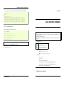
An example: calculating the laplacian
image[1:-1, 1:-1] = (image[:-2, 1:-1] - image[2:, 1:-1] +
image[1:-1, :-2] - image[1:-1, 2:])*0.25
In
In
In
In
In
[3]:
[4]:
[5]:
[6]:
[7]:
With integer arrays
• Example: sorting a vector with another one:
import pylab as pl
l = sp.lena()
pl.imshow(l, cmap=pl.cm.gray)
e = l[:-2, 1:-1] - l[2:, 1:-1] + l[1:-1, :-2] - l[1:-1, 2:]
pl.imshow(e, cmap=pl.cm.gray)
>>> a, b = np.random.random_integers(10, size=(2, 4))
>>> a
array([8, 6, 2, 9])
>>> b
array([ 8, 9, 3, 10])
>>> a_order = np.argsort(a)
>>> a_order
array([2, 1, 0, 3])
>>> b[a_order]
array([ 3, 9, 8, 10])
Using masks
• Zeroing out all the even elements of a table:
>>> a = np.arange(10)
>>> a
array([0, 1, 2, 3, 4, 5, 6, 7, 8, 9])
>>> a[(a % 2) == 1] = 0
>>> a
array([1, 3, 5, 7, 9])
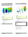
• Applying a mask to a grid to select the center of an image:
In
In
In
In
In
[8]: n, m = l.shape
[9]: x, y = np.indices((n, m))
[10]: distance = np.sqrt((x - 0.5*n)**2 + (y - 0.5*m)**2)
[11]: l[distance > 200] = 255
[12]: pl.imshow(l, cmap=pl.cm.gray)
Timing ratio
3.1.2 Advanced indexing
With integers or masks
3.1. Numpy: array computing
34
3.1. Numpy: array computing
35
Introduction to Python for Science, Release 1
Introduction to Python for Science, Release 1
3.1.3 Broadcasting
Multidimensional operations
• You can add a numer to an array:
>>> a =
>>> a
array([
>>> a +
array([
Using broadcasting for performance
np.ones((3, ))
1.,
1
2.,
1.,
1.])
2.,
2.])
• Creating a 3D grid
• And what if we add two arrays of different shapes?
>>> b = 2*np.ones((2, 1))
>>> b
array([[ 2.],
[ 2.]])
>>> a + b
array([[ 3., 3., 3.],
[ 3., 3., 3.]])
• Dimensions are matched:
np.sqrt(x**2 + y**2 + z**2)
3.1. Numpy: array computing
36
3.1. Numpy: array computing
37
Introduction to Python for Science, Release 1
Introduction to Python for Science, Release 1
With broadcasting
>>> x, y, z = np.ogrid[-100:100, -100:100, -100:100]
>>> print x.shape, y.shape, z.shape
(200, 1, 1) (1, 200, 1) (1, 1, 200)
>>> r = np.sqrt(x**2 + y**2 + z**2)
Without broadcasting
>>> x, y, z = np.mgrid[-100:100, -100:100, -100:100]
>>> print x.shape, y.shape, z.shape
(200, 200, 200) (200, 200, 200) (200, 200, 200)
>>> r = np.sqrt(x**2 + y**2 + z**2)
• Timing: 1.1s: creating x, y, z: 6ms
• Memory: x, y, z : 1.6Kb. r : 64Mo, and one 64Mo temporary array
• Timing: 2.3s: creating x, y, z: 0.5s, calculation of r: 1.8s
=> 120Mb
• Memory : 64Mo per array, 6 arrays, (x, y, z, r) and 2 temporary arrays
• 16 million operations
=> 400Mb
• 200^3 floating point operations per array:
numpy: a structured view on memory, with associated operations
48 million operations.
•
•
•
•
•
identical data type (dtype)
fast indexing
views and copies
costless reshape
shape-aware operations (broadcasting)
3.2 Matplotlib : scientific 2D plotting
Matplotlib: provides a matlab-like plotting interface, pylab
Note: Reference: the documentation is excellent: http://matplotlib.sourceforge.net/
3.1. Numpy: array computing
38
3.2. Matplotlib : scientific 2D plotting
39
Introduction to Python for Science, Release 1
Introduction to Python for Science, Release 1
3.2.1 Lines
import numpy as np
import pylab as pl
from scipy.special import jn
x = np.linspace(-5, 15, 100)
for i in range(10):
y = jn(i, x)
pl.plot(x, y, label=’$j_%i$’ % i)
pl.title(’Fonctions de Bessel’)
pl.legend()
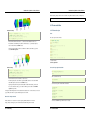
3.2.3 Points
import numpy as np
import pylab as pl
x, y, value = np.random.normal(size=(3, 50))
pl.scatter(x, y, np.abs(50*value), c=value)
3.2.2 2D arrays
import scipy as sp
import pylab as pl
l = sp.lena()
pl.imshow(l, cmap=pl.cm.gray)
pl.axis(’off’)
3.2.4 Vectors
import numpy as np
import pylab as pl
x, y = np.mgrid[-5:5, -5:5]
u = -x
3.2. Matplotlib : scientific 2D plotting
40
3.2. Matplotlib : scientific 2D plotting
41
Introduction to Python for Science, Release 1
v = y
pl.quiver(x, y, u, v)
Introduction to Python for Science, Release 1
np.loadtxt/np.savetxt
• Clever loading of text/csv files:
np.genfromtxt/np.recfromcsv
• Fast an efficient binary format:
np.save/np.load
3.3.2 Optimization
• Finding zeros of a function:
>>> def f(x):
...
return x**3 - x**2 - 10
>>> from scipy import optimize
>>> optimize.fsolve(f, 1)
2.5445115283877615
• Curve fitting:
3.3 Scipy: numerical and scientific toolbox
import numpy as np
import pylab as pl
from scipy import optimize
scipy is mainly composed of task-specific sub-modules:
cluster
fftpack
integrate
interpolate
io
linalg
maxentropy
ndimage
odr
optimize
signal
sparse
spatial
special
stats
Vector quantization / Kmeans
Fourier transform
Integration routines
Interpolation
Data input and output
Linear algebra routines
Routines for fitting maximum entropy models
n-dimensional image package
Orthogonal distance regression
Optimization
Signal processing
Sparse matrices
Spatial data structures and algorithms
Any special mathematical functions
Statistics
x = np.linspace(0, 10, 100)
y = np.sin(x) + 0.5*np.random.normal(size=100)
pl.plot(x, y, ’.’)
def test_func(x, a, f, phi):
return a*np.sin(f*x+phi)
(a, f, phi), _ = optimize.curve_fit(test_func, x, y)
pl.plot(x, test_func(x, a, f, phi), ’--’, linewidth=3)
3.3.1 IO
• Load and save matlab files:
>>> from scipy import io
>>> struct = io.loadmat(’file.mat’, struct_as_record=True)
>>> io.savemat(’file.mat’, struct)
See also:
• Load text files:
3.3. Scipy: numerical and scientific toolbox
42
3.3. Scipy: numerical and scientific toolbox
43
Introduction to Python for Science, Release 1
Introduction to Python for Science, Release 1
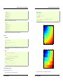
3.3.4 Image processing
from scipy import ndimage
l = sp.lena()
pl.imshow(ndimage.gaussian_filter(l, 5), cmap=pl.cm.gray)
pl.imshow(ndimage.gaussian_gradient_magnitude(l, 3), cmap=pl.cm.gray)
3.3.5 Interpolation
3.3.3 Statistics and random numbers
>>> a = np.random.normal(size=1000)
>>> bins = np.arange(-4, 5)
>>> bins
array([-4, -3, -2, -1, 0, 1, 2, 3, 4])
>>> histogram = np.histogram(a, bins=bins)
>>> bins = 0.5*(bins[1:] + bins[:-1])
>>> bins
array([-3.5, -2.5, -1.5, -0.5, 0.5, 1.5, 2.5,
>>> from scipy import stats
>>> b = stats.norm.pdf(bins)
x = np.arange(10)
y = np.sin(x)
pl.plot(x, y, ’+’, markersize=10)
from scipy import interpolate
f = interpolate.interp1d(x, y)
X = np.linspace(0, 9, 100)
pl.plot(X, f(X), ’--’)
3.5])
f = interpolate.interp1d(x, y, kind=’cubic’)
X = np.linspace(0, 9, 100)
pl.plot(X, f(X), ’--’)
In [1]: pl.plot(bins, histogram)
In [2]: pl.plot(bins, b)
3.3. Scipy: numerical and scientific toolbox
44
3.3. Scipy: numerical and scientific toolbox
45
Introduction to Python for Science, Release 1
3.3.6 Interlude
Introduction to Python for Science, Release 1
3.3.8 FFT
Low pass filtering:
import scipy as sp
import numpy as np
import pylab as pl
import numpy as np
import pylab as pl
from scipy import fftpack
l = sp.lena()
l = l[235:235+153, 205:162+205]
t = np.arange(0, 10, 0.1)
t = pl.imread(’tarek.jpg’)
t = t[::-1, ...]
t = t.sum(axis=-1)
s = np.sin(np.pi*t) + np.cos(10*np.pi*t)
pl.plot(t, s)
pl.figure()
pl.imshow(t, cmap=pl.cm.gray)
pl.axis(’off’)
freq = fftpack.fftfreq(len(s), d=.1)
fft = fftpack.fft(s)
fft[np.abs(freq) > 1] = 0
s_ = fftpack.ifft(fft)
pl.figure()
pl.imshow(l, cmap=pl.cm.gray)
pl.axis(’off’)
pl.plot(t, s_, linewidth=3)
t = t.astype(np.float)
t /= t.max()
l = l.astype(np.float)
l /= l.max()
pl.figure()
pl.imshow(t + l, cmap=pl.cm.gray)
pl.axis(’off’)
3.3.7 Lineaire Algebra
3.3.9 Signal processing
“whitening” Lena:
• Detrend:
rows, weight, columns = np.linalg.svd(l, full_matrices=False)
l_ = np.dot(rows, columns)
import numpy as np
import pylab as pl
from scipy import signal
t = np.linspace(0, 5, 100)
x = t + np.random.normal(size=100)
pl.plot(t, x, linewidth=3)
pl.plot(t, signal.detrend(x), linewidth=3)
3.3. Scipy: numerical and scientific toolbox
46
3.3. Scipy: numerical and scientific toolbox
47
Introduction to Python for Science, Release 1
CHAPTER 4
Python patterns in neuro image
• Filtering:
Ground truth:
Noisy observation:
4.1 Images and Mask
l = sp.lena()[200:-100, 150:-150]
l = l/float(l.max())
g = l + .1*np.random.normal(size=l.shape)
An fMRI dataset: 4D array, (x, y, z, t)
im = np.random.random((8, 9, 10, 11))
A mask (ROI, or brain): 3D array, (x, y, z)
mask = (np.random.random((8, 9, 10)) > .5)
Corresponding time series: 2D array, (voxel, t)
time_series = im[mask]
Gaussian filter:
Median filter:
Wiener filter:
4.2 Memory management
ndimage.gaussian_filter(g, 1.6)
• In place operations:
signal.medfilt2d(g, 5)
time_series -= time_series.mean(axis=-1)[:, np.newaxis]
time_series /= time_series.std(axis=-1)[:, np.newaxis]
signal.wiener(g, (5, 5))
• For loops rather than axis:
from scipy import signal
for time_serie in time_series:
time_serie[:] = signal.detrend(time_serie)
Note: time_serie is a view on time_series. time_serie[:] gives an in-place operation.
• memmapping (np.load):
np.save(’time_series.npy’, time_series)
time_series = np.load(’time_series.npy’, mmap_mode=’r’)
3.3. Scipy: numerical and scientific toolbox
48
49
Introduction to Python for Science, Release 1
Introduction to Python for Science, Release 1
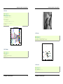
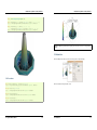
4.4 Dealing with labels
Warning: memmap object: read-only
• ndimage.labels:
4.3 Masked arrays
l = sp.lena()[200:300, 230:360]
pl.imshow(l, cmap=pl.cm.gray)
Data, with many dimensions/parameters: subject, session, ROI, time:
data = np.ones((3, 4, 10)) # subject, ROI, time
But: missing data, crapy data, (babies anyone?):
bad_data = np.zeros(data.shape, dtype=np.bool)
# For subject 0, ROI 1 is outside of brain
bad_data[0, 1, :] = True
# Subject 1 moved between time 3 and 5:
bad_data[1, :, 3:6] = True
blacks = l < 80
pl.imshow(blacks, cmap=pl.cm.gray)
“Mask” the bad data: masked arrays (np.ma):
good_data = np.ma.masked_array(data, mask=bad_data)
How many useful ROIs:
>>> good_data.sum(axis=1)
masked_array(data =
[[3.0 3.0 3.0 3.0 3.0 3.0 3.0 3.0 3.0 3.0]
[4.0 4.0 4.0 -- -- -- 4.0 4.0 4.0 4.0]
[4.0 4.0 4.0 4.0 4.0 4.0 4.0 4.0 4.0 4.0]],
mask =
[[False False False False False False False False False False]
[False False False True True True False False False False]
[False False False False False False False False False False]],
fill_value = 1e+20)
from scipy import ndimage
label_im, labels = ndimage.label(blacks)
imshow(label_im, cmap=pl.cm.spectral)
What’s the mean across time, not counting bad data:
masked_array(data =
[[1.0 -- 1.0 1.0]
[1.0 1.0 1.0 1.0]
[1.0 1.0 1.0 1.0]],
mask =
[[False True False False]
[False False False False]
[False False False False]],
fill_value = 1e+20)
• ndimage.mean, ndimage.maximum, ndimage.maximum_position...:
means = ndimage.mean(l, labels=label_im, index=range(labels))
Clean up small connect components:
labels
size =
for s,
if
Note: Much better than NaNs, the above would not be possible.
Note: Also good for thresholding maps.
4.3. Masked arrays
50
= np.arange(labels)
ndimage.sum(blacks, labels=label_im, index=labels)
index in zip(size, labels):
s < 40:
label_im[label_im == index] = 0
4.4. Dealing with labels
51
Introduction to Python for Science, Release 1
CHAPTER 5
• Reassign labels np.searchsorted:
3D plotting with Mayavi
labels = np.unique(label_im)
label_im = np.searchsorted(labels, label_im)
• ndimage.center_of_mass:
>>> ndimage.center_of_mass(label_im.astype(np.float),
label_im.astype(np.float), index=labels)
[(nan, nan),
(14.303212851405622, 8.6425702811244989),
(6.0357142857142856, 24.910714285714285),
(62.170854271356781, 33.984924623115575),
(nan, nan),
(nan, nan)]
• ndimage.find_objects:
slice_x, slice_y = ndimage.find_objects(label_im==4)[0]
eye = l[slice_x, slice_y]
pl.imshow(eye, cmap=pl.cm.gray)
5.1 A simple example
Warning: Start ipython -wthread
4.4. Dealing with labels
52
53
Introduction to Python for Science, Release 1
Introduction to Python for Science, Release 1
5.2.2 Lines
In [5]: mlab.clf()
In [6]: t = np.linspace(0, 20, 200)
In [7]: mlab.plot3d(np.sin(t), np.cos(t), 0.1*t, t)
Out[7]: <enthought.mayavi.modules.surface.Surface object at 0xcc3e1dc>
import numpy as np
x, y = np.mgrid[-10:10:100j, -10:10:100j]
r = np.sqrt(x**2 + y**2)
z = np.sin(r)/r
from enthought.mayavi import mlab
mlab.surf(z, warp_scale=’auto’)
mlab.outline()
mlab.axes()
np.mgrid[-10:10:100j, -10:10:100j]: Create an x,y grid, going from -10 to 10, with 100 steps in each directions.
5.2 3D plotting functions
5.2.1 Points
In [1]: import numpy as np
5.2.3 Elevation surface
In [2]: from enthought.mayavi import mlab
In [8]: mlab.clf()
In [3]: x, y, z, value = np.random.random((4, 40))
In [9]: x, y = np.mgrid[-10:10:100j, -10:10:100j]
In [4]: mlab.points3d(x, y, z, value)
Out[4]: <enthought.mayavi.modules.glyph.Glyph object at 0xc3c795c>
In [10]: r = np.sqrt(x**2 + y**2)
In [11]: z = np.sin(r)/r
In [12]: mlab.surf(z, warp_scale=’auto’)
Out[12]: <enthought.mayavi.modules.surface.Surface object at 0xcdb98fc>
5.2. 3D plotting functions
54
5.2. 3D plotting functions
55
Introduction to Python for Science, Release 1
Introduction to Python for Science, Release 1
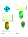
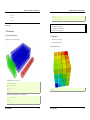
5.2.5 Volumetric data
In [20]: mlab.clf()
In [21]: x, y, z = np.mgrid[-5:5:64j, -5:5:64j, -5:5:64j]
In [22]: values = x*x*0.5 + y*y + z*z*2.0
In [23]: mlab.contour3d(values)
Out[24]: <enthought.mayavi.modules.iso_surface.IsoSurface object at 0xcfe392c>
5.2.4 Arbitrary regular mesh
In [13]: mlab.clf()
In [14]: phi, theta = np.mgrid[0:pi:11j, 0:2*pi:11j]
In [15]: x = sin(phi)*cos(theta)
In [16]: y = sin(phi)*sin(theta)
In [17]: z = cos(phi)
In [18]: mlab.mesh(x, y, z)
This function works with a regular orthogonal grid:
In [19]: mlab.mesh(x, y, z, representation=’wireframe’, color=(0, 0, 0))
Out[19]: <enthought.mayavi.modules.surface.Surface object at 0xce1017c>
Note: A surface is defined by points connected to form triangles or polygones. In mlab.func and mlab.mesh, the
connectivity is implicity given by the layout of the arrays. See also mlab.triangular_mesh.
Our data is often more than points and values: it needs some connectivity information
5.2. 3D plotting functions
56
5.2. 3D plotting functions
57
Introduction to Python for Science, Release 1
Introduction to Python for Science, Release 1
5.3 Figures and decorations
Example docstring: mlab.mesh
5.3.1 Figure management
Plots a surface using grid-spaced data supplied as 2D arrays.
Function signatures:
mesh(x, y, z, ...)
Get the current figure:
Clear the current figure:
Set the current figure:
Save figure to image file:
Change the view:
x, y, z are 2D arrays, all of the same shape, giving the positions of the vertices of the surface. The connectivity
between these points is implied by the connectivity on the arrays.
For simple structures (such as orthogonal grids) prefer the surf function, as it will create more efficient data
structures.
Keyword arguments:
color the color of the vtk object. Overides the colormap, if any, when specified. This is
specified as a triplet of float ranging from 0 to 1, eg (1, 1, 1) for white.
colormap type of colormap to use.
extent [xmin, xmax, ymin, ymax, zmin, zmax] Default is the x, y, z arrays extents. Use
this to change the extent of the object created.
figure Figure to populate.
line_width The with of the lines, if any used. Must be a float. Default: 2.0
mask boolean mask array to suppress some data points.
mask_points If supplied, only one out of ‘mask_points’ data point is displayed. This
option is usefull to reduce the number of points displayed on large datasets Must be
an integer or None.
mode the mode of the glyphs. Must be ‘2darrow’ or ‘2dcircle’ or ‘2dcross’ or
‘2ddash’ or ‘2ddiamond’ or ‘2dhooked_arrow’ or ‘2dsquare’ or ‘2dthick_arrow’
or ‘2dthick_cross’ or ‘2dtriangle’ or ‘2dvertex’ or ‘arrow’ or ‘cone’ or ‘cube’ or
‘cylinder’ or ‘point’ or ‘sphere’. Default: sphere
name the name of the vtk object created.
representation the representation type used for the surface. Must be ‘surface’ or ‘wireframe’ or ‘points’ or ‘mesh’ or ‘fancymesh’. Default: surface
resolution The resolution of the glyph created. For spheres, for instance, this is the
number of divisions along theta and phi. Must be an integer. Default: 8
scalars optional scalar data.
scale_factor scale factor of the glyphs used to represent the vertices, in fancy_mesh
mode. Must be a float. Default: 0.05
scale_mode the scaling mode for the glyphs (‘vector’, ‘scalar’, or ‘none’).
transparent make the opacity of the actor depend on the scalar.
tube_radius radius of the tubes used to represent the lines, in mesh mode. If None,
simple lines are used.
tube_sides number of sides of the tubes used to represent the lines. Must be an integer.
Default: 6
vmax vmax is used to scale the colormap If None, the max of the data will be used
vmin vmin is used to scale the colormap If None, the min of the data will be used
mlab.gcf()
mlab.clf()
mlab.figure(1, bgcolor=(1, 1, 1), fgcolor=(0.5, 0.5, 0.5)
mlab.savefig(‘foo.png’, size=(300, 300))
mlab.view(azimuth=45, elevation=54, distance=1.)
5.3.2 Changing plot properties
Example:
In [1]: import numpy as np
In [2]: r, theta = np.mgrid[0:10, -np.pi:np.pi:10j]
In [3]: x = r*np.cos(theta)
In [4]: y = r*np.sin(theta)
In [5]: z = np.sin(r)/r
5.3. Figures and decorations
58
5.3. Figures and decorations
59
Introduction to Python for Science, Release 1
Introduction to Python for Science, Release 1
In [6]: from enthought.mayavi import mlab
In [7]: mlab.mesh(x, y, z, colormap=’gist_earth’, extent=[0, 1, 0, 1, 0, 1])
Out[7]: <enthought.mayavi.modules.surface.Surface object at 0xde6f08c>
In [8]: mlab.mesh(x, y, z, extent=[0, 1, 0, 1, 0, 1],
...: representation=’wireframe’, line_width=1, color=(0.5, 0.5, 0.5))
Out[8]: <enthought.mayavi.modules.surface.Surface object at 0xdd6a71c>
Warning: extent: If we specified extents for a plotting object, mlab.outline’ and ‘mlab.axes don’t get them by
default.
5.4 Interaction
Click on the ‘Mayavi’ button in the scene, and you can control properties of objects with dialogs.
5.3.3 Decorations
In [9]: mlab.colorbar(Out[7], orientation=’vertical’)
Out[9]: <tvtk_classes.scalar_bar_actor.ScalarBarActor object at 0xd897f8c>
Click on the red button, and it generates lines of code.
In [10]: mlab.title(’polar mesh’)
Out[10]: <enthought.mayavi.modules.text.Text object at 0xd8ed38c>
In [11]: mlab.outline(Out[7])
Out[11]: <enthought.mayavi.modules.outline.Outline object at 0xdd21b6c>
In [12]: mlab.axes(Out[7])
Out[12]: <enthought.mayavi.modules.axes.Axes object at 0xd2e4bcc>
5.3. Figures and decorations
60
5.4. Interaction
61
Introduction to Python for Science, Release 1
CHAPTER 6
• Modify values of variables.
• Set breakpoints.
Ways to launch the debugger:
1. Postmortem, launch debugger after module errors.
2. Enable debugger in ipython and automatically drop into debug-mode on error.
3. Launch the module with the debugger.
Debugging
6.2.1 Postmortem
Situation: You’re working in ipython and you get a traceback.
Type %debug and drop into the debugger.
In [6]: run index_error.py
--------------------------------------------------------------------------IndexError
Traceback (most recent call last)
The python debugger pdb: http://docs.python.org/library/pdb.html
/Users/cburns/src/scipy2009/scipy_2009_tutorial/source/index_error.py in <module>()
6
7 if __name__ == ’__main__’:
----> 8
index_error()
9
10
6.1 Coding best practices to avoid getting in trouble
Brian Kernighan
“Everyone knows that debugging is twice as hard as writing a program in the first place. So if you’re as clever
as you can be when you write it, how will you ever debug it?”
/Users/cburns/src/scipy2009/scipy_2009_tutorial/source/index_error.py in index_error()
3 def index_error():
4
lst = list(’foobar’)
----> 5
print lst[len(lst)]
6
7 if __name__ == ’__main__’:
• We all write buggy code. Accept it. Deal with it.
• Write your code with testing and debugging in mind.
• Keep It Simple, Stupid (KISS).
IndexError: list index out of range
WARNING: Failure executing file: <index_error.py>
– What is the simplest thing that could possibly work?
• Don’t Repeat Yourself (DRY).
– Every piece of knowledge must have a single, unambiguous, authoritative representation within a system.
– Constants, algorithms, etc...
In [7]: %debug
> /Users/cburns/src/scipy2009/scipy_2009_tutorial/source/index_error.py(5)index_error()
4
lst = list(’foobar’)
----> 5
print lst[len(lst)]
6
• Try to limit interdependencies of your code. (Loose Coupling)
ipdb> list
1 """Small snippet to raise an IndexError."""
2
3 def index_error():
4
lst = list(’foobar’)
----> 5
print lst[len(lst)]
6
7 if __name__ == ’__main__’:
8
index_error()
• Give your variables, functions and modules meaningful names.
6.2 The debugger
A debugger allows you to inspect your code interactively.
Specifically it allows you to:
• View the source code.
ipdb> len(lst)
6
ipdb> print lst[len(lst)-1]
r
• Walk up and down the call stack.
• Inspect values of variables.
62
6.2. The debugger
63
Introduction to Python for Science, Release 1
ipdb> quit
17
18 if __name__ == ’__main__’:
19
data = load_data(’exercises/data.txt’)
20
print(’min: %f’ % min(data)) # 10.20
21
print(’max: %f’ % max(data)) # 61.30
In [8]:
6.2.2 Debugger launch
Continue execution to next breakpoint with c(ont(inue)):
Situation: You believe a bug exists in a module but are not sure where.
Launch the module with the debugger and step through the code in the debugger.
In [38]: run -d debug_file.py
*** Blank or comment
*** Blank or comment
Breakpoint 1 at /Users/cburns/src/scipy2009/scipy_2009_tutorial/source/debug_file.py:3
NOTE: Enter ’c’ at the ipdb> prompt to start your script.
> <string>(1)<module>()
Step into code with s(tep):
ipdb> step
--Call-> /Users/cburns/src/scipy2009/scipy_2009_tutorial/source/debug_file.py(4)<module>()
1
3 Data is stored in data.txt.
----> 4 """
5
ipdb> break load_data
Breakpoint 2 at /Users/cburns/src/scipy2009/scipy_2009_tutorial/source/debug_file.py:12
ipdb> break
Num Type
Disp Enb
Where
1
breakpoint
keep yes
at /Users/cburns/src/scipy2009/scipy_2009_tutorial/source/debug_file.py:3
2
breakpoint
keep yes
at /Users/cburns/src/scipy2009/scipy_2009_tutorial/source/debug_file.py:12
I don’t want to debug python’s open function, so use the n(ext) command to continue execution on the next line:
ipdb> next
> /Users/cburns/src/scipy2009/scipy_2009_tutorial/source/debug_file.py(14)load_data()
13
fp = open(filename)
---> 14
data_string = fp.read()
15
fp.close()
ipdb> next
> /Users/cburns/src/scipy2009/scipy_2009_tutorial/source/debug_file.py(16)load_data()
15
fp.close()
---> 16
return parse_data(data_string)
17
Step into parse_data function with s(tep) command:
ipdb> step
--Call-> /Users/cburns/src/scipy2009/scipy_2009_tutorial/source/debug_file.py(6)parse_data()
5
----> 6 def parse_data(data_string):
7
data = []
List the code with l(ist):
ipdb> list
1 """Script to read in a column of numbers and calculate the min, max and sum.
2
1
3 Data is stored in data.txt.
----> 4 """
5
6 def parse_data(data_string):
7
data = []
8
for x in data_string.split(’.’):
9
data.append(x)
10
return data
11
ipdb> list
1 """Script to read in a column of numbers and calculate the min, max and sum.
2
1
3 Data is stored in data.txt.
4 """
5
----> 6 def parse_data(data_string):
7
data = []
8
for x in data_string.split(’.’):
9
data.append(x)
10
return data
11
load_data(filename):
fp = open(filename)
data_string = fp.read()
fp.close()
return parse_data(data_string)
6.2. The debugger
ipdb> continue
> /Users/cburns/src/scipy2009/scipy_2009_tutorial/source/debug_file.py(13)load_data()
2
12 def load_data(filename):
---> 13
fp = open(filename)
14
data_string = fp.read()
ipdb> next
> /Users/cburns/src/scipy2009/scipy_2009_tutorial/source/debug_file.py(15)load_data()
14
data_string = fp.read()
---> 15
fp.close()
16
return parse_data(data_string)
Set a breakpoint at the load_data function:
ipdb> list
2
12 def
13
14
15
16
Introduction to Python for Science, Release 1
Continue stepping through code and print out values with the p(rint) command:
64
6.2. The debugger
65
Introduction to Python for Science, Release 1
ipdb> step
> /Users/cburns/src/scipy2009/scipy_2009_tutorial/source/debug_file.py(9)parse_data()
8
for x in data_string.split(’.’):
----> 9
data.append(x)
10
return data
ipdb> p x
’10’
ipdb> s
> /Users/cburns/src/scipy2009/scipy_2009_tutorial/source/debug_file.py(8)parse_data()
7
data = []
----> 8
for x in data_string.split(’.’):
9
data.append(x)
ipdb> s
> /Users/cburns/src/scipy2009/scipy_2009_tutorial/source/debug_file.py(9)parse_data()
8
for x in data_string.split(’.’):
----> 9
data.append(x)
10
return data
Introduction to Python for Science, Release 1
ipdb> down
> /Users/cburns/src/scipy2009/scipy_2009_tutorial/source/debug_file.py(9)parse_data()
8
for x in data_string.split(’.’):
----> 9
data.append(x)
10
return data
ipdb> list
4 """
5
6 def
7
8
----> 9
10
11
2
12 def
13
14
parse_data(data_string):
data = []
for x in data_string.split(’.’):
data.append(x)
return data
load_data(filename):
fp = open(filename)
data_string = fp.read()
ipdb>
ipdb> p x
’2\n43’
6.3 print
You can also walk up and down the call stack with u(p) and d(own):
ipdb> list
4 """
5
6 def
7
8
----> 9
10
11
2
12 def
13
14
Yes, print statements do work as a debugging tool.
6.4 Debugging strategies
parse_data(data_string):
data = []
for x in data_string.split(’.’):
data.append(x)
return data
1. Make it fail reliably. Find a test case that makes the code fail every time.
2. Divide and Conquer. Once you have a failing test case, isolate the failing code.
load_data(filename):
fp = open(filename)
data_string = fp.read()
• Which module.
• Which function.
ipdb> up
> /Users/cburns/src/scipy2009/scipy_2009_tutorial/source/debug_file.py(16)load_data()
15
fp.close()
---> 16
return parse_data(data_string)
17
2. Take notes. It may take a while.
3. Be patient. It may take a while.
4. Purposely raise an exception where you believe the problem is, to inspect the code via the debuger (eg ‘%debug’
in IPython)
ipdb> list
11
2
12 def load_data(filename):
13
fp = open(filename)
14
data_string = fp.read()
15
fp.close()
---> 16
return parse_data(data_string)
17
18 if __name__ == ’__main__’:
19
data = load_data(’exercises/data.txt’)
20
print(’min: %f’ % min(data)) # 10.20
21
print(’max: %f’ % max(data)) # 61.30
6.2. The debugger
• Which line of code.
1. Change one thing at a time and re-run the failing test case.
66
6.3. print
67
Introduction to Python for Science, Release 1
CHAPTER 7
def test():
data = np.random.random((5000, 100))
u, s, v = linalg.svd(data)
pca = np.dot(u[:10, :], data)
results = fastica(pca.T, whiten=False)
test()
Profiling Python code
In [1]: %run -t demo.py
IPython CPU timings (estimated):
User :
14.3929 s.
System:
0.256016 s.
In [2]: %run -p demo.py
916 function calls in 14.551 CPU seconds
Ordered by: internal time
No optimization without measuring!
ncalls
1
1
1
54
2
6
6
14
19
1
1
107
7
7
172
1
29
35
35
21
41
28
1
25
19
21
7
41
13
9
28
14
23
7
14
14
• Measure: profiling, timing
• “Premature optimization is the root of all evil”
7.1 Timeit
In IPython, to time elementatry operations:
In [1]: import numpy as np
In [2]: a = np.arange(1000)
In [3]: %timeit a**2
100000 loops, best of 3: 5.73 us per loop
In [4]: %timeit a**2.1
1000 loops, best of 3: 154 us per loop
In [5]: %timeit a*a
100000 loops, best of 3: 5.56 us per loop
7.2 Profiler
Useful when you have a large program to profile.
import numpy as np
from scipy import linalg
from ica import fastica
@profile
68
tottime
14.457
0.054
0.017
0.011
0.005
0.001
0.001
0.001
0.001
0.001
0.001
0.000
0.000
0.000
0.000
0.000
0.000
0.000
0.000
0.000
0.000
0.000
0.000
0.000
0.000
0.000
0.000
0.000
0.000
0.000
0.000
0.000
0.000
0.000
0.000
0.000
7.2. Profiler
percall
14.457
0.054
0.017
0.000
0.002
0.000
0.000
0.000
0.000
0.001
0.001
0.000
0.000
0.000
0.000
0.000
0.000
0.000
0.000
0.000
0.000
0.000
0.000
0.000
0.000
0.000
0.000
0.000
0.000
0.000
0.000
0.000
0.000
0.000
0.000
0.000
cumtime
14.479
0.054
0.021
0.011
0.005
0.001
0.001
0.001
0.001
0.008
14.551
0.001
0.004
0.002
0.000
14.551
0.000
0.000
0.001
0.001
0.000
0.000
0.008
0.000
0.000
0.000
0.000
0.000
0.000
0.000
0.000
0.000
0.000
0.000
0.000
0.000
percall
14.479
0.054
0.021
0.000
0.002
0.000
0.000
0.000
0.000
0.008
14.551
0.000
0.001
0.000
0.000
14.551
0.000
0.000
0.000
0.000
0.000
0.000
0.008
0.000
0.000
0.000
0.000
0.000
0.000
0.000
0.000
0.000
0.000
0.000
0.000
0.000
filename:lineno(function)
decomp.py:849(svd)
{method ’random_sample’ of ’mtrand.RandomState’ objects}
function_base.py:645(asarray_chkfinite)
{numpy.core._dotblas.dot}
{method ’any’ of ’numpy.ndarray’ objects}
ica.py:195(gprime)
ica.py:192(g)
{numpy.linalg.lapack_lite.dsyevd}
twodim_base.py:204(diag)
ica.py:69(_ica_par)
{execfile}
defmatrix.py:239(__array_finalize__)
ica.py:58(_sym_decorrelation)
linalg.py:841(eigh)
{isinstance}
demo.py:1(<module>)
numeric.py:180(asarray)
defmatrix.py:193(__new__)
defmatrix.py:43(asmatrix)
defmatrix.py:287(__mul__)
{numpy.core.multiarray.zeros}
{method ’transpose’ of ’numpy.ndarray’ objects}
ica.py:97(fastica)
{abs}
{numpy.core.multiarray.arange}
defmatrix.py:527(getT)
linalg.py:64(_commonType)
{len}
{max}
{method ’view’ of ’numpy.ndarray’ objects}
{method ’get’ of ’dict’ objects}
linalg.py:36(isComplexType)
{issubclass}
linalg.py:92(_fastCopyAndTranspose)
{method ’astype’ of ’numpy.ndarray’ objects}
linalg.py:49(_realType)
69
Introduction to Python for Science, Release 1
7
7
7
1
1
7
15
7
6
0.000
0.000
0.000
0.000
0.000
0.000
0.000
0.000
0.000
0.000
0.000
0.000
0.000
0.000
0.000
0.000
0.000
0.000
0.000
0.000
0.000
0.000
0.000
0.000
0.000
0.000
0.000
0.000
0.000
0.000
0.000
0.000
0.000
0.000
0.000
0.000
CHAPTER 8
{numpy.core.multiarray._fastCopyAndTranspose}
linalg.py:31(_makearray)
linalg.py:110(_assertSquareness)
lapack.py:63(get_lapack_funcs)
lapack.py:48(find_best_lapack_type)
linalg.py:104(_assertRank2)
{min}
{method ’__array_wrap__’ of ’numpy.ndarray’ objects}
defmatrix.py:521(getA)
Advanced numpy
7.3 Line-profiler
@profile
def test():
data = np.random.random((5000, 100))
u, s, v = linalg.svd(data)
pca = np.dot(u[:10, :], data)
results = fastica(pca.T, whiten=False)
Optimising numpy code
1. avoiding loops
2. algorithmic optimisation (eg. not doing the same thing more than once)
3. memory/number of operations minimization and trade-off
~ $ kernprof.py -l -v demo.py
Wrote profile results to demo.py.lprof
Timer unit: 1e-06 s
Avoiding loops
• Fancy indexing
File: demo.py
Function: test at line 5
Total time: 14.2793 s
• Know the numpy library well
• Reshaping, striding
Line #
Hits
Time Per Hit
% Time Line Contents
==============================================================
5
@profile
6
def test():
7
1
19015 19015.0
0.1
data = np.random.random((5000, 100))
8
1
14242163 14242163.0
99.7
u, s, v = linalg.svd(data)
9
1
10282 10282.0
0.1
pca = np.dot(u[:10, :], data)
10
1
7799
7799.0
0.1
results = fastica(pca.T, whiten=False)
• Think different
Algorithmic optimisation
• See the forest, not the trees:
– Think before you code
– Refactor
• Know the standard scientific library (scipy)
The SVD is taking all the time. We need to optimise this ligne.
– http://docs.scipy.org/
In [3]: %timeit np.linalg.svd(data)
1 loops, best of 3: 14.5 s per loop
– numpy.lookfor
• Know your math:
In [4]: from scipy import linalg
wrong:
In [5]: %timeit linalg.svd(data)
1 loops, best of 3: 14.2 s per loop
import numpy as np
_, singular_values, _ = np.linalg.svd(np.dot(X.T, X))
In [6]: %timeit linalg.svd(data, full_matrices=False)
1 loops, best of 3: 295 ms per loop
harder, better, faster stronger:
In [7]: %timeit np.linalg.svd(data, full_matrices=False)
1 loops, best of 3: 293 ms per loop
from scipy import linalg
singular_values = sp.linalg.eigvalsh(np.dot(X.T, X))
Minimize memory/number of operations
7.3. Line-profiler
70
71
Introduction to Python for Science, Release 1
• Views and copies
Introduction to Python for Science, Release 1
>>> a + b
array([[ 3.,
[ 3.,
• Broadcasting
• Fancy indexing
3.,
3.,
3.],
3.]])
Broadcasting rules:
Table of Contents
• Element-wize operations on arrays:
• Compare dimensions, starting from last
• Dimension of size 1 are extrapolated.
8.1 Broadcasting
8.1.1 Broadcasting definition
8.1.2 Applications
Applying operators on arrays of different shapes:
• Yet another way of avoiding loops
• Decreases memory consumption
Creating a 3D grid of size n
• Adding a scalar and an array of course works:
>>> import numpy as np
>>> a = np.ones((3, ))
>>> a
array([ 1., 1., 1.])
>>> a + 1
array([ 2., 2., 2.])
np.sqrt(x**2 + y**2 + z**2)
• What about adding (or multiplying) two arrays of different shape?
>>> b = 2*np.ones((2, 1))
>>> b
array([[ 2.],
[ 2.]])
8.1. Broadcasting
72
8.1. Broadcasting
73
Introduction to Python for Science, Release 1
Introduction to Python for Science, Release 1
With broadcasting, sample n values for each A, B, X and Y, along a different direction each time. n^4 samples for f.
Warning: Unwanted correlations are introduced between the random variables.
8.2 Views and strides
8.2.1 Views and copies
Without broadcasting
>>> x, y, z = np.mgrid[-100:100, -100:100, -100:100]
>>> print x.shape, y.shape, z.shape
(200, 200, 200) (200, 200, 200) (200, 200, 200)
>>> r = np.sqrt(x**2 + y**2 + z**2)
Views
These three lines take 2.3s: the creation of x, y, z takes 0.5s, and the calculation of r takes 1.8s.
>>> import numpy as np
>>> a = np.arange(10)
>>> a
array([0, 1, 2, 3, 4, 5, 6, 7, 8, 9])
>>> b = a[3:7]
>>> b
array([3, 4, 5, 6])
>>> b[0] = 0
>>> b
array([0, 4, 5, 6])
>>> a
array([0, 1, 2, 0, 4, 5, 6, 7, 8, 9])
Two arrays can point to the same data:
The total memory used is 64Mb per array. There are 4 named arrays (x, y, z) and at least 2 temporary
arrays are created. Thus around 400Mb are used.
Squaring each array take 200^3 operations, as well as the two additions, and the call to np.sqrt. Thus
a total of 48 million operations.
a was also modified.
No memory duplication
With broadcasting
How to tell: inspecting the data buffer
>>> x, y, z = np.ogrid[-100:100, -100:100, -100:100]
>>> print x.shape, y.shape, z.shape
(200, 1, 1) (1, 200, 1) (1, 1, 200)
>>> r = np.sqrt(x**2 + y**2 + z**2)
• >>> np.may_share_memory(a, b)
True
• The base attribute of the array:
These lines take 1.1s second, with only 6ms to create the arrays.
>>> b.base is a
True
The three input arrays take only 1.6Kb. The output array 64Mb, and there is not more than a 64Mb
and a 320kb temporary array created. Around 120Mb are used.
• Look at the base pointer of the data buffer, and the extent:
Squaring each array takes 200 operations, the first addition is 200^2 = 40 thousands operations, and
the second, as well as the call to np.sqrt, is 200^3 = 8 million operations. Thus around 16 million
operations are performed.
Looking at the relative timings between non-broadcasted and broadcasted versions, we can see that they do not scale
proportionally to the number of operations. Broadcasting does take some time.
Monte-Carlo density evaluation
Density evaluation of f = A sin(k1 X) + B sin(k2 Y) using the probability distribution of A, B, X and Y.
a.ctypes.data
140052096
a.ctypes.data + len(a.data)
140052136
b.ctypes.data
140052108
b.ctypes.data + len(b.data)
140052124
• Look at the ‘OWNDATA’ flag to tell if the array owns its data:
Strategy: sample f with huge arrays of the random variables, and build an histogram of the results.
8.1. Broadcasting
74
8.2. Views and strides
75
Introduction to Python for Science, Release 1
>>> b.flags
C_CONTIGUOUS : True
F_CONTIGUOUS : True
OWNDATA : False
WRITEABLE : True
ALIGNED : True
UPDATEIFCOPY : False
Introduction to Python for Science, Release 1
import numpy as np
import pylab as pl
x, y = np.ogrid[0:10, 0:10]
r = np.sqrt(x**2 + y**2)
pl.matshow(r)
r_binned = r.reshape((5, 2, 5, 2)).sum(axis=-1).sum(axis=1)
pl.matshow(r_binned)
But this does not mean another array shares the data:
>>> del a
>>> b.flags
C_CONTIGUOUS : True
F_CONTIGUOUS : True
OWNDATA : False
WRITEABLE : True
ALIGNED : True
UPDATEIFCOPY : False
The base data container is not cleared as long as there are views opened on it.
Applications
• With a mask:
>>> a = np.arange(10)
>>> a
array([0, 1, 2, 3, 4, 5, 6, 7, 8, 9])
>>> a[(a % 2) == 0] = 0
>>> a
array([0, 1, 0, 3, 0, 5, 0, 7, 0, 9])
A view was created: an array of shape (5, ), and all the elements were set to zero (through Broadcasting of 0 to
a (5, )-shaped array).
• In loops:
>>> a = np.arange(30).reshape((3, 10))
>>> a
array([[ 0, 1, 2, 3, 4, 5, 6, 7, 8, 9],
[10, 11, 12, 13, 14, 15, 16, 17, 18, 19],
[20, 21, 22, 23, 24, 25, 26, 27, 28, 29]])
>>> from scipy.signal import detrend
>>> for line in a:
...
line[:] = detrend(line)
>>> a
array([[0, 0, 0, 0, 0, 0, 0, 0, 0, 0],
[0, 0, 0, 0, 0, 0, 0, 0, 0, 0],
[0, 0, 0, 0, 0, 0, 0, 0, 0, 0]])
8.2.2 Reshaping, striding
Reshaping can be a special case of views.
• To understand this better, let us consider what happens to the first line:
• You can do unusual operations on arrays along certain strides:
8.2. Views and strides
76
8.2. Views and strides
77
Introduction to Python for Science, Release 1
>>> r[:, 0]
array([ 0., 1., 2., 3., 4., 5., 6.,
>>> r[:, 0].reshape((5, 2))
array([[ 0., 1.],
[ 2., 3.],
[ 4., 5.],
[ 6., 7.],
[ 8., 9.]])
>>> r[:, 0].reshape((5, 2)).sum(axis=-1)
array([ 1.,
5.,
9., 13., 17.])
7.,
8.,
Introduction to Python for Science, Release 1
Take home message:
9.])
You can apply operations with ‘a certain regularity’ on an array by finding the view that gives you the right
striding and shape.
8.2.3 In place operations
• Inplace operators (*=)
• All ufuncs take an out arguments.
• Reshaping is (when possible) just a matter of changing the stride and shape for a flat array:
Without inplace operations
>>> r = np.arange(8)
>>> r.strides
(4,)
>>> r.shape
(8,)
>>> x = np.linspace(-100, 100, 1e6)
>>> y = np.linspace(-100, 100, 1e6)
>>> r = np.sqrt(x**2 + y**2)
Time of the calculation of r: 2s
Using inplace operations All ufunc take an out argument:
>>>
>>>
>>>
>>>
**= 2
**= 2
+= y
= np.sqrt(x, x)
Total time: 1.4s
After reshape:
>>>
>>>
(8,
>>>
(4,
x
y
x
r
Memory consumption twice as small.
r2 = r.reshape((4, 2))
r2.strides
4)
r2.shape
2)
In conclusion:
views (eventually strided) avoid memory consumption, and open the door to interesting array manipulations
8.3 Fancy indexing
8.3.1 Rules
Indexing with integer arrays
>>> import numpy as np
>>> a = np.arange(30).reshape((3, -1))
>>> a
array([[ 0, 1, 2, 3, 4, 5, 6, 7, 8, 9],
[10, 11, 12, 13, 14, 15, 16, 17, 18, 19],
[20, 21, 22, 23, 24, 25, 26, 27, 28, 29]])
>>> a[:, (1, 3)]
array([[ 1, 3],
[11, 13],
[21, 23]])
And when slicing backwards:
>>> r3 = r[::-1]
>>> r3.strides
(-4,)
8.2. Views and strides
78
8.3. Fancy indexing
79
Introduction to Python for Science, Release 1
Introduction to Python for Science, Release 1
Shape is given by (shape of indexing array) * slices:
>>> indices = np.random.randint(a.shape[-1],
>>> indices
array([[3, 6, 5, 4, 8, 9, 1, 7, 9, 6],
[8, 0, 5, 0, 9, 6, 2, 0, 5, 2],
[6, 3, 7, 0, 9, 0, 3, 2, 3, 1]])
>>> bootstrap = a[:, indices]
>>> bootstrap
array([[[ 3, 6, 5, 4, 8, 9, 1, 7, 9,
[ 8, 0, 5, 0, 9, 6, 2, 0, 5,
[ 6, 3, 7, 0, 9, 0, 3, 2, 3,
<BLANKLINE>
[[13, 16, 15, 14, 18, 19, 11, 17, 19,
[18, 10, 15, 10, 19, 16, 12, 10, 15,
[16, 13, 17, 10, 19, 10, 13, 12, 13,
>>> a[:, ((1, 3), (2, 4))].shape
(3, 2, 2)
If multiple integer arrays for indexing, they are broadcasted together:
>>> a[(1, 2), ((1, ), (2, ))]
array([[11, 21],
[12, 22]])
Indexing with boolean arrays
>>> a[(a%2)==0]
array([ 0, 2, 4,
6,
8, 10, 12, 14, 16, 18, 20, 22, 24, 26, 28])
6,
6],
2],
1]],
16],
12],
11]]])
Now we can do vectorized computations easily on the bootstraped sample.
Flat shape. Slicing not used:
>>> a[:, (a%2)==0]
array([ 0, 2, 4,
size=(3, 10))
Extracting a cut of volume along a horizon
8, 10, 12, 14, 16, 18, 20, 22, 24, 26, 28])
We have an image (volumetric data):
8.3.2 Applications
>>> image = np.random.randint(10, size=(5, 5))
>>> image
array([[3, 1, 3, 7, 1],
[7, 4, 0, 5, 1],
[5, 9, 9, 4, 0],
[9, 8, 8, 6, 8],
[6, 3, 1, 2, 5]])
Rearranging vectors
We have a vector family:
>>> vectors =
>>> vectors
array([[2, 8,
[5, 9,
[0, 8,
[1, 1,
np.random.randint(10, size=(4, 5))
2,
2,
6,
6,
1,
4,
5,
1,
And a horizon: the coordinates of a curve in the image:
7],
6],
3],
1]])
>>> horizon = np.array([3, 2, 1, 3, 2])
We can extract the value on the horizon:
We want to rearrange them by variance:
>>> image[horizon, np.arange(5)]
array([9, 9, 0, 6, 0])
>>> variance = np.var(vectors, axis=0)
>>> variance
array([ 3.5
, 10.25 ,
4.
,
3.1875,
5.6875])
>>> rearranged = vectors[:, np.argsort(variance)]
>>> np.var(rearranged, axis=0)
array([ 3.1875,
3.5
,
4.
,
5.6875, 10.25 ])
Local average along a horizon
This time, we want to extract the voxels in the 3-voxels-wide region around the horizon:
>>> image[horizon +
array([[5, 4, 3, 4,
[9, 9, 0, 6,
[6, 8, 9, 2,
Bootstrapping
We have a vector a:
Two broadcastings: one in x coordinates horizon + np.arange(-1, 2)[:, np.newaxis], and the second one between the x
and the y coordinates.
>>> a = np.arange(20).reshape((2, 10))
>>> a
array([[ 0, 1, 2, 3, 4, 5, 6, 7, 8, 9],
[10, 11, 12, 13, 14, 15, 16, 17, 18, 19]])
Drawback of these techniques: costly in memory
We want to drawn three times 10 vectors out of a:
8.3. Fancy indexing
np.arange(-1, 2)[:, np.newaxis], np.arange(5)]
1],
0],
8]])
80
8.3. Fancy indexing
81
Introduction to Python for Science, Release 1
CHAPTER 9
8.4 Robert (Kern)’s nasty stride trick
Warning: Parents guidance: not for underaged children
Problem Sliding average, but we don’t want copies.
We want to take a sliding average of a, on a window of size 2:
pyflakes: fast static analysis
>>> import numpy as np
>>> a = np.arange(8)
>>> a
array([0, 1, 2, 3, 4, 5, 6, 7])
>>> a.strides
(4,)
We are going to create improbable strides and shapes (numpy 1.2):
• Fast, simple
>>> from numpy.lib import stride_tricks
>>> b = stride_tricks.as_strided(a, shape=(2, 7), strides=(4, 4))
>>> b
array([[0, 1, 2, 3, 4, 5, 6],
[1, 2, 3, 4, 5, 6, 7]])
• Detects syntax errors, missing imports, typos on names.
9.1 In kate
Menu: ‘settings -> configure kate -> External Tools’, add pyflakes:
Overlapping dimensions!
Easy, now all we have to do is sum along the axis 0:
>>> b.sum(axis=0)
array([ 1, 3, 5,
7,
9.2 In vim
9, 11, 13])
In your .vimrc (binds F5 to pyflakes):
autocmd
autocmd
autocmd
autocmd
8.4. Robert (Kern)’s nasty stride trick
82
FileType
FileType
FileType
FileType
python let &mp = ’echo "*** running % ***" ; pyflakes %’
tex,mp,rst,python imap <Esc>[15~ <C-O>:make!^M
tex,mp,rst,python map <Esc>[15~ :make!^M
tex,mp,rst,python set autowrite
83
Introduction to Python for Science, Release 1
9.3 In emacs
In your .emacs (binds F5 to pyflakes):
(defun pyflakes-thisfile () (interactive)
(compile (format "pyflakes %s" (buffer-file-name)))
)
(define-minor-mode pyflakes-mode
"Toggle pyflakes mode.
With no argument, this command toggles the mode.
Non-null prefix argument turns on the mode.
Null prefix argument turns off the mode."
;; The initial value.
nil
;; The indicator for the mode line.
" Pyfalkes"
;; The minor mode bindings.
’( ([f5] . pyflakes-thisfile) )
)
(add-hook ’python-mode-hook (lambda () (pyflakes-mode t)))
9.3. In emacs
84