Download RUG LaTEX Course

RUG LaTEX Course
Siep Kroonenberg
RUG LaTEX Course, version 1.1 December 2015
Created for the Faculty of Economics and Business of the University of Groningen
email:
Copyright © 2015 Siep Kroonenberg
Copying and distribution of this file, with or without modification, are permitted in any medium without royalty provided the copyright notice and this notice are preserved. This file is offered as-is, without any warranty.
Contents
Preface
1
2
3
4
5
3
Introduction
1.1 History . . . . . . . . . . . . . . . . . . . .
1.2 The TEX/LaTEX ecosystem . . . . . . . . . .
1.3 Working with LaTEX . . . . . . . . . . . . .
Getting started
2.1 Getting (La)TEX . . . . . . . . . . . . . . .
2.2 The RuG TEX Live launcher . . . . . . . . .
2.3 Next: let the system display file extensions
2.4 TeXstudio . . . . . . . . . . . . . . . . . .
2.5 First document . . . . . . . . . . . . . . . .
2.6 Documentation . . . . . . . . . . . . . . .
2.7 Practice files . . . . . . . . . . . . . . . . .
.
.
.
.
.
.
.
.
.
.
.
.
.
.
.
.
.
.
.
.
.
.
.
.
.
.
.
.
.
.
.
.
.
.
.
.
.
.
.
.
.
.
.
.
.
.
.
.
.
.
.
.
.
.
.
.
.
.
.
.
.
.
.
.
.
.
.
.
.
.
.
.
.
.
.
.
.
.
.
.
.
.
.
.
.
.
.
.
.
.
.
.
.
.
.
.
.
.
.
.
.
.
.
.
.
.
.
.
.
.
.
.
.
.
.
.
.
.
.
.
.
.
.
.
.
.
.
.
.
.
.
.
.
6
6
6
7
8
8
9
10
Basics
3.1 Paragraphs . . . . . . . . . . . . . . . . .
3.2 Comments . . . . . . . . . . . . . . . . .
3.3 Control sequences and -characters . . . .
3.4 Grouping . . . . . . . . . . . . . . . . . .
3.5 Text formatting . . . . . . . . . . . . . .
3.6 Special characters . . . . . . . . . . . . .
3.7 Lists: itemize, enumerate and description
3.8 LaTEX classes . . . . . . . . . . . . . . . .
3.9 Sectioning commands . . . . . . . . . . .
3.10 Title . . . . . . . . . . . . . . . . . . . . .
3.11 Footnotes and ‘thanks’ . . . . . . . . . .
3.12 Practice . . . . . . . . . . . . . . . . . . .
.
.
.
.
.
.
.
.
.
.
.
.
.
.
.
.
.
.
.
.
.
.
.
.
.
.
.
.
.
.
.
.
.
.
.
.
.
.
.
.
.
.
.
.
.
.
.
.
.
.
.
.
.
.
.
.
.
.
.
.
.
.
.
.
.
.
.
.
.
.
.
.
.
.
.
.
.
.
.
.
.
.
.
.
.
.
.
.
.
.
.
.
.
.
.
.
.
.
.
.
.
.
.
.
.
.
.
.
.
.
.
.
.
.
.
.
.
.
.
.
.
.
.
.
.
.
.
.
.
.
.
.
.
.
.
.
.
.
.
.
.
.
.
.
.
.
.
.
.
.
.
.
.
.
.
.
.
.
.
.
.
.
.
.
.
.
.
.
.
.
.
.
.
.
.
.
.
.
.
.
.
.
.
.
.
.
.
.
.
.
.
.
.
.
.
.
.
.
.
.
.
.
.
.
.
.
.
.
.
.
.
.
.
.
.
.
.
.
.
.
.
.
.
.
.
.
.
.
.
.
.
.
.
.
.
.
.
.
.
.
11
11
11
11
12
12
12
13
14
14
15
15
16
Math
4.1 Amsmath . . . . . . . . . . . . . . .
4.2 Math mode: Inline and display math
4.3 Mathematical notation . . . . . . .
4.4 Various constructs . . . . . . . . . .
4.5 Arrays/matrices . . . . . . . . . . .
4.6 Multiline equations . . . . . . . . .
4.7 Fonts in math . . . . . . . . . . . .
4.8 Macros . . . . . . . . . . . . . . . .
4.9 Practice . . . . . . . . . . . . . . . .
.
.
.
.
.
.
.
.
.
.
.
.
.
.
.
.
.
.
.
.
.
.
.
.
.
.
.
.
.
.
.
.
.
.
.
.
.
.
.
.
.
.
.
.
.
.
.
.
.
.
.
.
.
.
.
.
.
.
.
.
.
.
.
.
.
.
.
.
.
.
.
.
.
.
.
.
.
.
.
.
.
.
.
.
.
.
.
.
.
.
.
.
.
.
.
.
.
.
.
.
.
.
.
.
.
.
.
.
.
.
.
.
.
.
.
.
.
.
.
.
.
.
.
.
.
.
.
.
.
.
.
.
.
.
.
.
.
.
.
.
.
.
.
.
.
.
.
.
.
.
.
.
.
.
.
.
.
.
.
.
.
.
.
.
.
.
.
.
.
.
.
.
.
.
.
.
.
.
.
.
17
17
17
17
18
19
20
21
21
22
Tabulars
5.1 Basics . . . . . . . . . . . . . . . . . . . . . . . . . . . . . . . . . . . . . . . .
5.2 Partial rules . . . . . . . . . . . . . . . . . . . . . . . . . . . . . . . . . . . .
5.3 Multicolumn . . . . . . . . . . . . . . . . . . . . . . . . . . . . . . . . . . . .
23
23
24
24
DECEMBER 2015
.
.
.
.
.
.
.
.
.
.
.
.
.
.
.
.
.
.
.
.
.
.
.
.
.
.
.
. . . . . . . . . . . . . . . . . . .
. . . . . . . . . . . . . . . . . . .
. . . . . . . . . . . . . . . . . . .
4
4
4
4
1
CONTENTS
5.4
5.5
5.6
5.7
5.8
.
.
.
.
.
.
.
.
.
.
.
.
.
.
.
.
.
.
.
.
.
.
.
.
.
.
.
.
.
.
.
.
.
.
.
.
.
.
.
.
.
.
.
.
.
.
.
.
.
.
.
.
.
.
.
.
.
.
.
.
.
.
.
.
.
.
.
.
.
.
.
.
.
.
.
.
.
.
.
.
.
.
.
.
.
.
.
.
.
.
.
.
.
.
.
.
.
.
.
.
24
25
25
25
26
Graphics
6.1 External graphics . . . . . . . . . . . . . .
6.2 Producers of graphic files . . . . . . . . . .
6.3 Including an external graphics file . . . . .
6.4 Floating figures and tables . . . . . . . . .
6.5 Practice documents for graphics and floats
.
.
.
.
.
.
.
.
.
.
.
.
.
.
.
.
.
.
.
.
.
.
.
.
.
.
.
.
.
.
.
.
.
.
.
.
.
.
.
.
.
.
.
.
.
.
.
.
.
.
.
.
.
.
.
.
.
.
.
.
.
.
.
.
.
.
.
.
.
.
.
.
.
.
.
.
.
.
.
.
.
.
.
.
.
.
.
.
.
.
.
.
.
.
.
27
27
29
29
30
31
Presentations
7.1 Alternatives . . . . . . . . .
7.2 Getting started with Beamer
7.3 Slides are frames . . . . . . .
7.4 Title frame . . . . . . . . . .
7.5 Themes . . . . . . . . . . . .
7.6 Modes . . . . . . . . . . . .
7.7 What about sections? . . . .
7.8 Figures and tables . . . . . .
7.9 Practice . . . . . . . . . . . .
.
.
.
.
.
.
.
.
.
.
.
.
.
.
.
.
.
.
.
.
.
.
.
.
.
.
.
.
.
.
.
.
.
.
.
.
.
.
.
.
.
.
.
.
.
.
.
.
.
.
.
.
.
.
.
.
.
.
.
.
.
.
.
.
.
.
.
.
.
.
.
.
.
.
.
.
.
.
.
.
.
.
.
.
.
.
.
.
.
.
.
.
.
.
.
.
.
.
.
.
.
.
.
.
.
.
.
.
.
.
.
.
.
.
.
.
.
.
.
.
.
.
.
.
.
.
.
.
.
.
.
.
.
.
.
.
.
.
.
.
.
.
.
.
.
.
.
.
.
.
.
.
.
.
.
.
.
.
.
.
.
.
.
.
.
.
.
.
.
.
.
32
32
32
32
33
33
34
34
34
34
A Changing the appearance
A.1 Empty lines instead of paragraph indentation .
A.2 Double-spacing . . . . . . . . . . . . . . . . .
A.3 Display math alignment . . . . . . . . . . . . .
A.4 Page dimensions . . . . . . . . . . . . . . . . .
A.5 Font size . . . . . . . . . . . . . . . . . . . . .
A.6 Fonts . . . . . . . . . . . . . . . . . . . . . . .
.
.
.
.
.
.
.
.
.
.
.
.
.
.
.
.
.
.
.
.
.
.
.
.
.
.
.
.
.
.
.
.
.
.
.
.
.
.
.
.
.
.
.
.
.
.
.
.
.
.
.
.
.
.
.
.
.
.
.
.
.
.
.
.
.
.
.
.
.
.
.
.
.
.
.
.
.
.
.
.
.
.
.
.
.
.
.
.
.
.
.
.
.
.
.
.
.
.
.
.
.
.
35
35
35
35
36
36
36
B Language support
B.1 Babel . . . . . . . . . . . . . . . . . . . . . . . . . . . . . . . . . . . . . . . .
B.2 Non-western scripts with XeTeX and LuaTeX . . . . . . . . . . . . . . . . . .
38
38
38
C Bibliographic references
C.1 The why and how of BibTEX . . . . . . . . . . . . . . . . . . . . .
C.2 nocite: entries without citations . . . . . . . . . . . . . . . . . . .
C.3 Bibliography styles: three generations . . . . . . . . . . . . . . . .
C.4 Generating your own bibliography style with custom-bib/makebst
C.5 The latest and greatest: biblatex . . . . . . . . . . . . . . . . . . .
C.6 The BibTEX database format . . . . . . . . . . . . . . . . . . . . .
C.7 BibTEX editors and bibliography managers . . . . . . . . . . . . .
C.8 Examples . . . . . . . . . . . . . . . . . . . . . . . . . . . . . . . .
C.9 The url field . . . . . . . . . . . . . . . . . . . . . . . . . . . . . .
C.10 Practice . . . . . . . . . . . . . . . . . . . . . . . . . . . . . . . . .
C.11 Troubleshooting . . . . . . . . . . . . . . . . . . . . . . . . . . . .
39
39
40
41
42
43
44
45
46
48
49
49
6
7
Decimal alignment
Text columns . . . .
Floating tables . . .
Importing table data
Practice . . . . . . .
References
2
.
.
.
.
.
.
.
.
.
.
.
.
.
.
.
.
.
.
.
.
.
.
.
.
.
.
.
.
.
.
.
.
.
.
.
.
.
.
.
.
.
.
.
.
.
.
.
.
.
.
.
.
.
.
.
.
.
.
.
.
.
.
.
.
.
.
.
.
.
.
.
.
.
.
.
.
.
.
.
.
.
.
.
.
.
.
.
.
.
.
.
.
.
.
.
.
.
.
.
.
.
.
.
.
.
.
.
.
.
.
.
.
.
.
.
.
.
.
.
.
.
.
.
.
.
.
.
.
.
.
.
.
.
.
.
.
.
.
.
.
.
.
.
.
.
.
.
.
.
.
.
.
.
.
.
.
.
.
.
.
.
.
.
.
.
.
.
.
.
.
.
.
.
.
.
.
.
.
.
.
.
.
.
.
.
.
.
.
.
.
.
.
.
.
.
.
.
.
51
RUG LATEX COURSE
Preface
This book accompanies a LaTEX introduction for first-year econometrics students at the
Rijksuniversiteit Groningen. It is just a quick introduction, but lists various more in-depth
resources.
Appendices contain additional topics which I consider too important to omit but which
do not fit in with a quick introduction. Consult them as needed.
There is an accompanying downloadable zip file with sample code.
The first chapter tells a bit about the background and philosophy of LaTEX.
The second chapter deals with practicalities such as setting up your own TEX environment.
It also introduces the ready-to-run TEX installation of the Rijksuniversiteit Groningen.
The TeXstudio editor used in the introduction is free, cross-platform and has palettes of
mathematical symbols to facilitate coding mathematics for new LaTEX users. But most of
this book is editor-agnostic, and the launcher, see below, makes it easy to switch editors.
The university installation and the TEX Live launcher
A few words about our local setup: the university’s TEX Live installation resides on the
network. It includes a launcher with menu entries for the various components of the installation. Upon first use the launcher does some initialization, such as adjusting the searchpath
and setting up file associations. Note that with a private TEX Live installation, these tasks
would already have been done by the installer. You can rerun this initializer at any time if
something seems messed up.
For ease of maintenance, the new 2015 edition of the launcher reads its menu and file
associations from an ini file. I intend to make this launcher publicly available at some later
date.
Until that happens, you can find a predecessor of the launcher at www.tug.org/texlive/
w32client.html. This is an initialization script which creates a menu and file associations,
and adds TEX Live to the user searchpath. It is a batch file / Perl script combination which
makes use of the built-in Perl of TEX Live.
DECEMBER 2015
3
1
Introduction
This book is just an introduction: it tries to teach you enough to get you started and explore
LaTEX further on your own, and hopefully let you see the advantages of doing things the
LaTEX way.
This chapter gives a bit of background.
1.1 History
LaTEX is pretty old, and its roots are even older.
In 1977 Donald Knuth, a mathematician, started creating his typesetting system TEX as a
tool for better typesetting, expecially of mathematics. The first version of TEX appeared in
1978. The second version, which was a complete rewrite, appeared in 1982.
The TEX system is based on a markup language. Contrary to html, another popular
markup language, TEX is designed for precision typesetting of complex texts, and is also
a macro programming language.
In the early 1980s Leslie Lamport provided a set of macros providing features such as
automatic chapter- and section numbering, footnotes and automatic cross-referencing.
LaTEX allows authors to concentrate on the meaning and structure of documents, rather
on appearance. This is called structural markup. If used well, structural markup makes for a
faster, less error-prone publishing process.
There are LaTEX templates or classfiles for most uses of TEX: besides articles, reports and
books, slides and letters are also provided for. Most TEX users started using the LaTEX system
for their documents, adding their own stuff as needed, rather than starting their own macro
package from scratch.
1.2 The TEX/LaTEX ecosystem
TEX and LaTEX caught on, and a large ecosystem grew up around it. Users around the world
contributed macros, fonts, support for non-Western languages, manuals and utilities. The
vast majority is free.
The CTAN archives are the main repository for TEX-related material, but quite possibly
your TEX installation already contains everything you need, or provides an easy way to add
the missing pieces.
The sites of TEX user groups such as http://www.tug.org/ and http://www.ntg.nl/
host various mailing lists and have links to other TEX- and LaTEX-related sites. I maintain
my own site http://tex.aanhet.net/rugtex/ about the RuG TEX installation.
1.3 Working with LaTEX
LaTEX is not a wysywyg wordprocessor. Preparing a document with LaTEX is a three-step
cycle:
1. Enter your text, with markup, in a text editor such as Notepad or TeXstudio or Emacs.
2. ‘Compile’ your document, i.e. convert it to pdf; more on that later.
4
RUG LATEX COURSE
1.3
Working with LaTEX
3. Preview it in a pdf viewer such as Adobe Reader or SumatraPDF or the pdf viewer built
into the editor, if there is one.
Below you see a marked-up source fragment at the left and two typeset results at the right:
1.1
\subsection{Some mathematics}\label{math}
The econometric model is confronted with observed
data and the parameters are estimated by
econometric techniques, as shown in equation
\ref{eq:smm} below:
\begin{equation}
Y_t = G_1 (Y, X, \hat{\Theta}, \hat{U})
\label{eq:smm}
\end{equation}
Some mathematics
The econometric model is confronted
with observed data and the parameters are estimated by econometric
techniques, as shown in equation 1
below:
Yt = G1 (Y, X, Θ̂, Û )
(1)
1.1 Some mathematics. The econometric model is confronted with observed data and the parameters are
estimated by econometric techniques,
as shown in equation 1 below:
Yt = G1 (Y, X, Θ̂, Û)
(1)
The difference in appearance is entirely due to changes in the document header: you can set
up the global layout once and for all, and then just focus on the text itself.
LaTEX excels at automatic numbering and cross-referencing; as well as at other longdocument features such as bibliographies and indexing. This machinery works efficiently
and reliably whatever the size of the project.
DECEMBER 2015
5
2
Getting started
2.1 Getting (La)TEX
2.1.1 Editor
An obvious component of a (La)TEX installation is the editor in which you enter your documents, and which compiles them into pdf files. For this introduction we use the TeXstudio
editor, which is free, and is available for Windows, Mac OS X and Linux. It offers extensive
assistance for entering LaTEX code and math.
Since LaTEX files are plain text files, you can view them in any editor, but it is important
to edit them in an editor which adds nothing binary. You can use a general programmers
editor or even Notepad, but an editor which understands LaTEX can give you a lot more help.
2.1.2 TEX system
The editor is actually the least important part; it delegates all the hard work to the TEX
system in the background.
A TEX system is a complex ensemble of command-line programs, macros, fonts and data
files. The two major alternatives are TEX Live and MiKTEX, both free. The RuG installation
uses TEX Live, which is available for Windows, Mac OS and Unix/Linux, and is included in
most Linux distributions. The other one, MiKTEX, is Windows-only. Both contain all the
bits and pieces that you are likely to need, although TEX Live is a bit more comprehensive.
They both include the TeXworks editor.
2.1.3 More advice
My a website http://tex.aanhet.net/rugtex/ contains a page which goes into more detail
about putting together your own TEX system. There are also download links. Another useful
beginners resource is http://www.tug.org/begin.html.
Two important points:
• Make sure TEX Live or MiKTEX is installed before you run the editor for the first time. This
enables the editor to configure itself automatically for your TEX system.
• A full LaTEX install takes a long time; do not attempt this, e.g., while in class.
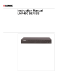
2.2 The RuG TEX Live launcher
The ready-to-run LaTEX installation at the Rijksuniversiteit Groningen is based on TEX Live
and contains several editors and utilities, some of which will be mentioned later in this book.
Figure 2.1. The TEX Live launcher
6
RUG LATEX COURSE
2.3
Next: let the system display file extensions
Figure 2.2. Letting Windows display file extensions
For a standard university UWP computer, you should have a menu item Start / Programs /
Text Processing / TeX Live RuG yyyy. This invokes the RuG TEX Live Launcher, see Figure 2.1.
The RuG TEX Live launcher is also available in a remote session. From this launcher you can
start up your favorite LaTEX editor, consult documentation and do some configuration and
maintenance. Take a moment to browse the launcher menus.
The ‘RuG TeX Live website’ item in the Online menu points to my website mentioned
earlier.
The button at the left, labeled ‘(La)TeX editor’, invokes your selected default editor. The
launcher offers you a couple of additional choices besides TeXstudio, plus the option to select
an editor of your own.
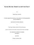
2.3 Next: let the system display file extensions
If you work on a file somefile.tex, then TEX is going to generate various auxiliary files such
as somefile.aux and somefile.log. If you want to tell such files apart, you need to configure
your computer to display file extensions. For Windows, you need the Folder Options dialog,
or File Explorer Options in Windows 10.
This dialog can be accessed via the Control Panel, in the ‘Appearance and Personalization’
category.1
Go to the View tab of the dialog, see figure 2.2, uncheck ‘Hide extensions for known file
types’ and click ‘OK’.
1. The Control Panel is slated to disappear from Windows 10 eventually. Other ways to open this dialog are via
Search, or via File Explorer, clicking first the View tab of the ribbon, then the Options button.
DECEMBER 2015
7
2
GETTING STARTED
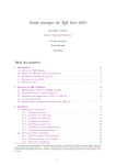
Figure 2.3. TeXstudio, a LaTEX editor. Left: structure; center top: editing area; center bottom: message
area; right: pdf preview
2.4 TeXstudio
Figure 2.3 shows the TeXstudio edit screen. The editing area is surrounded by various toolbars, a structure view on the left and, after a successful compilation, the built-in pdf viewer.
Optionally, there is also a tabbed message pane below the editing pane. This item is rather
useful. If you do not see it, you can make it visible by clicking on the second-left item at
the lower left corner of the editor window.
While you are at it, you can also right-click on an empty area of the toolbar or menu bar
to get rid of some of the toolbar clutter; everything is already available via the menus.
Also look through the TeXstudio menus, in particular:
• The Tools menu and its Commands submenu for running LaTEX and various utilities; see
section 2.5.
• The LaTeX menu for inserting various LaTEX macros
• The Math menu for inserting LaTEX macros for math
As you get to know LaTEX better, you may prefer to type LaTEX macros by hand.
2.5 First document
Now we are going to do the entire cycle: text entry, compilation and previewing in the LaTEX
editor TeXstudio. Create a new document by clicking on File / New and type the following
code:
\documentclass{article}
\begin{document}
Hello, world!
\end{document}
This is a complete LaTEX document. Setup is done in the preamble, i.e. the \documentclass
line and anything else before \begin{document}. In this case, we just specified that we
wanted an article rather than, e.g., a book or a letter. Actual content goes between
\begin{document} and \end{document}.
8
RUG LATEX COURSE
2.6
Documentation
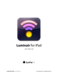
Figure 2.4. TeXstudio flagging errors
2.5.1 Compiling
Save the document as, e.g., X:\latexdocs\hello.tex. Then click the Build button ( ). If all
is well a pdf-preview pane should appear; see figure 2.3.
Also have a look at the message pane below the editing pane (figure 2.3). If there are
problems then TeXstudio tries to identify and flag the cause, see figure 2.4.
You can read more about compiling in Section 3 of the online help: Help / User Manual....
It also explains what to do in case of errors.
2.6 Documentation
Built-in help. The Help menu of TeXstudio provides both help for TeXstudio itself and a
LaTEX reference in html format.
The launcher Documentation- and Online menus contain shortcuts to several other useful
manuals and online resources.
The LaTeX Introduction menu entry points to a book-length introduction which covers all
the basics. It is also a nice demonstration of the bookmarking and hyperlinking that you get
virtually for free with LaTEX, and which makes the pdf very convenient to consult on-screen.
The next menu item, LaTeX Reference, is the TEX Live version of the above LaTEX reference,
also in pdf format and also fully bookmarked and hyperlinked.
The [UK TEX] FAQ is another useful resource.
2.6.1 The documentation list
You can gain access to documentation about packages in one of the following ways:
RUG Launcher In the Documentation menu, a menu item All TeX Live documentation by
package invokes an html file doc.html which contains links to virtually all package manuals.
Standard TeX Live The menu item Start / Programs / TeX Live nnnn / TeX Live Documentation invokes an html page which includes a link Available package documentation, which
is this same file.
MiKTeX lacks such a file, but you can still visit the CTAN Catalogue, http://mirror.ctan.
org/help/Catalogue/brief.html and consult package documentation there.
We shall refer to this list, however accessed, as ‘the documentation list.’
But you can also use the texdoc (TEX Live) or mthelp (MiKTEX) command-line utility.
2.6.2 Tip: view pdfs with narrow margins
For better use of your screen pixels, you may wish that your pdf viewer zoomed in on the
printed part of the page. Several pdf viewers can do this automatically. In Adobe Reader,
select View / Zoom / Fit Visible. In SumatraPDF, part of our TEX installation, select Zoom / Fit
Content.
DECEMBER 2015
9
2
GETTING STARTED
2.7 Practice files
This introduction comes with a zipfile practice.zip with some example .tex files, a subdirectory figures of graphic files for chapter 6 and a second subdirectory bibtex relating to
bibliography management in appendix C2 .
Several chapters conclude with suggestions for practicing, which usually refer to files
from this zipfile.
2.7.1 RUG TEX installation
The practice zipfile is the Practice files
item in the Documentation menu of the
launcher. If you click the item, you get to
see a folder named practice in a 7zip window. Drag-and-drop this folder to your X:drive. A destination on your desktop is
probably ok too.
2.7.2 Home TEX installation
The practice zipfile is available from CTAN in the info/latexcourse-rug
subdirectory. Right-click the zip file after downloading, select ‘Extract
All...’. Take care to pick some reasonable location, e.g. under Documents
or on the desktop. The default may well be some directory for temporary
files, which is probably not what you want.
2. This last topic is no longer part of the introduction. Nevertheless, the LaTEX bibliography system is highly
recommended.
10
RUG LATEX COURSE
3
Basics
Keep The Not So Short Introduction handy; as mentioned previously, it is in the launcher menu
under Documentation, or search for ‘lshort’ in the documentation list, see section 2.6.1.
Start a new LaTEX document as described in section 2.5, with content
\documentclass{article}
\begin{document}
Hello, world!
\end{document}
Hello, world!
You may already have guessed that macros start with \ and that a parameter can be enclosed
in braces { }. A construct \begin{something}...\end{something} is called an environment.
Now try out some of the syntax below on your new LaTEX document.
3.1 Paragraphs
You need to separate paragraphs with empty lines in the input file; a single linebreak is
equivalent to a space.
A linebreak in the source
A linebreak in the source creates a
creates a space in the pdf output.
space in the pdf output.
An empty line in the source ends a paraAn empty line in the source ends a paragraph.
graph.
3.2 Comments
The percent character, %, is the comment character; LaTEX ignores it and everything following it on the same line, including the linebreak itself.
one
%ignore
tw%
o
one two
3.3 Control sequences and -characters
LaTEX commands often take the form of a backslash followed by a series of letters, e.g.,
\LaTeX
LaTEX
A control sequence swallows succeeding spaces, so you sometimes have to follow it with {}
or ~:
\LaTeX code
\LaTeX~code, \LaTeX{} code, \LaTeX.
LaTEXcode
LaTEX code, LaTEX code, LaTEX.
Rendering control characters literally:
DECEMBER 2015
11
3
%
{ }
\
\\
function
comment character
parameter; grouping
starts control sequence
newline (!)
BASICS
render literally with
\%
\{ \}
\textbackslash
3.4 Grouping
A pair of braces can also localize the effect of a command:
x z {\footnotesize x z} x z
xzxzxz
3.5 Text formatting
The classfile and stylefiles will take care of many changes in text attributes, e.g., in section
heads and in bibliographies. Do not style these items manually. Appendix A contains some
simple recipes for global changes in appearance.
Below, we describe the more common commands for styling text.
3.5.1 Bold and italic
These commands work on all subsequent text within the current block:
normal \itshape italic \bfseries bolditalic
\upshape bold \mdseries normal
text italic bolditalic bold normal
Argument form:
normal \textit{italic} \textbf{bold}
normal italic bold
These are the basic text formatting commands:
‘from now on’
argument form
italic
upright
\itshape
\upshape
\textit{...}
\textup{...}
bold
medium
\bfseries
\mdseries
\textbf{...}
\textmd{...}
monospaced
\ttfamily
\texttt{...}
Some people recommend replacing \textit with \emph, which is short for emphasized, as
being more in line with structural markup.
TeXstudio has buttons for bold and italic on the inner vertical toolbar.
3.5.2 Text sizes
Predefined text sizes; note that some may come out the same:
\tiny
\scriptsize
\footnotesize
\small
\normalsize
\large
\Large
\LARGE
\huge
3.6 Special characters
Here a short list of typographic characters and how you can create them in LaTEX, even if
you use only typewriter characters in your input:
12
RUG LATEX COURSE
3.7
Lists: itemize, enumerate and description
Single quotes
Double quotes
Non-breaking space
Hyphen
En-dash
Em-dash
Accented characters
output
‘’
“”
–
—
é
ï
code
`'
``''
~
---\'e
\"\i
Using accented input characters requires loading the inputenc package in the preamble:1
\usepackage[utf8]{inputenc}
...
“ ä ï © « ” and `` \"a \"\i{} \textcopyright{} << ''
“ ä ï © « ” and “ ä ï © « ”
This method does not cover all unicode characters, and if you type a lot of code then you
may prefer control codes anyway.
For full unicode support, you should use the XeTEX or LuaTEX engines; see appendix sections A.6.1 and B.2.
3.6.1 Hyphens and dashes
Please be aware that not every horizontal dash is the same. A few examples of proper use:
En-dashes for ranges: 7--9 for ‘7–9’, or to set off – part of – a sentence.
Em-dashes also for setting off—part of—a sentence, but now without surrounding spaces2 .
A plain hyphen ‘-’ is appropriate for hyphenation and for compound words such as ‘crossreferencing’.
3.7 Lists: itemize, enumerate and description
Itemize (unnumbered list):
\begin{itemize}
\item camel
\item rabbit
\end{itemize}
• camel
• rabbit
Enumerate (numbered list):
\begin{enumerate}
\item soup
\item main course
\item dessert
\end{enumerate}
1. soup
2. main course
3. dessert
Description lists:
\begin{description}
\item[One] This is a short term.
\item[Quetzalqoatl] Mexican god, about whom we
could tell a lot if only we had the time and
inclination.
\end{description}
One This is a short term.
Quetzalqoatl Mexican god, about whom
we could tell a lot if only we had the
time and inclination.
1. latin1 (ISO-8859-1) and cp1252 (Windows-1252) are alternatives to utf8, but if we go beyond ASCII input at all,
utf8 (Unicode) is the more rational choice.
2. Or, better with thin spaces \,
DECEMBER 2015
13
3
BASICS
Lists can be nested:
\begin{enumerate}
\item soup
\item main course
\begin{itemize}
\item tortilla filled with meat and vegetables
\item[--] refried beans
\end{itemize}
\item dessert
\end{enumerate}
1. soup
2. main course
• tortilla filled with meat and
vegetables
– refried beans
3. dessert
Here a bad example of an item parameter. Since the item tag is an optional parameter, it uses
square brackets [ and ] rather than curly braces { and }.
3.8 LaTEX classes
Each LaTEX document starts with a \documentclass line, which selects a class file. Class files
define available features and a default look. Some important LaTEX document classes:
• article (no chapters)
• report
• book
The above classes are very similar in the features they support. You can add features or
change the appearance by loading packages:3
\documentclass[10pt,a4paper]{article}
\usepackage[utf8]{inputenc}
\usepackage{amsmath}
\usepackage{amsfonts}
\usepackage{amssymb}
3.9 Sectioning commands
The standard classes listed above have a predefined sectioning hierarchy: parts, chapters
(not for articles), sections, subsections, subsubsections, paragraphs and subparagraphs.
All these commands have an optional and a required parameter, e.g.
\section[Short title]{A very long and impossibly involved title,
which will never fit in a page header}
\subsection{A short enough title}
Sectioning titles may turn up in page headers or in an automatically generated table of contents. If a title is not short and simple, you should use an optional parameter which will not
cause trouble when it is reused in page headers or in a table of contents.
3.9.1 Bookmarks and clickable cross-references with hyperref
The hyperref package will create bookmarks from your sections, and also make all the crossreferences in your pdf clickable. Add an option colorlinks if you do not like the boxes
around links:
\usepackage[colorlinks]{hyperref}
3. This preamble is generated by the TeXstudio Quick Start wizard.
14
RUG LATEX COURSE
3.10
Title
3.10 Title
Publications customarily start with some sort of title page or -block. LaTEX creates such a
title with the \maketitle command. You should already have defined an author and title
with corresponding commands.
The \author- and \title commands can be placed either in the preamble or in the body
of the LaTEX source. The \maketitle command belongs in the body.
Here is an example of an article with a \usepackage command, a title block, a table of
contents and sections:
\documentclass{article}
\usepackage{newpxtext,newpxmath} % palatino font
\begin{document}
\title{Title of article}
\author{My name}
\maketitle
\thispagestyle{empty}
Title of article
My name
December 6, 2015
\tableofcontents
Contents
\section{A section}\label{sec:ASection}
1
See section \ref{sec:ASection} on page
\pageref{sec:ASection}.
\subsection{A subsection}
That's all, folks!
1
A section
1.1 A subsection . . . . . . . . . . . . .
1
1
A section
See section 1 on page 1.
1.1 A subsection
That’s all, folks!
\end{document}
Notice the use of cross-referencing commands \label, \ref and \pageref.
Warning. Cross-references usually require more than one (pdf)LaTEX run before they
are correctly resolved. This is also true for automatically generated text such as tables of
contents. After each LaTEX run you should check the message pane below the editing area
for errors and warnings.
3.11 Footnotes and ‘thanks’
In the LaTEX source footnotes are placed in the running text. The \footnote command generates both a mark in the running text and the footnote itself at the bottom. As with sectioning,
footnotes are numbered automatically:
Here comes a footnote.\footnote{%
This is the footnote.}
And some more text.
DECEMBER 2015
Here comes a footnote.1 And
some more text.
1 This
is the footnote.
15
3
BASICS
A special case is a footnote attached to the title or author of an article. Note that the footnote
should be inside the title- or author parameter.
Sample title∗
\title{Sample title\thanks{%
Supported by a grant}}
\author{A.U. Thor\thanks{%
And another grant}}
\maketitle
First line of regular text.\footnote{%
With a regular footnote.} And some more text.
A.U. Thor†
December 6, 2015
First line of regular text.1 And
some more text.
∗ Supported
by a grant
another grant
1 With a regular footnote.
† And
3.12 Practice
Start out with a new document as described in section 2.5. Use this document to try out the
code samples from this chapter.
If you feel ready to try bigger things, you can try to typeset some real text. If you
have nothing suitable of your own, you can turn to Wikipedia articles such as http://en.
wikipedia.org/wiki/Factors_of_production. You can copy-and-paste pieces of text from
the web page to your own LaTEX document.
Try to recreate the structure, not the appearance, e.g., use sectioning commands instead
of manually making headings bold, and let LaTEX create the table of contents. Also pay
attention to proper quotes and typographic characters.
Consult basics_sample.tex from the practice zip (see section 2.7) as an example of a
complete, structured LaTEX document.
16
RUG LATEX COURSE
4
Math
4.1 Amsmath
Although you can do a lot of math typesetting with LaTEX alone, we shall assume that
amsmath and related packages are loaded, e.g. with a command
\usepackage{amsmath,amsfonts,amssymb}
in the preamble, i.e. between \documentclass{. . . } and \begin{document}.
For documentation, click in the launcher Documentation / AmsMath User Guide, or search
the documentation list, see section 2.6.1.
4.2 Math mode: Inline and display math
Math in running text is bracketed between $ characters:1
Simple bits of math in running text,
enclosed in \$ characters: $x$ or
$\alpha$ or $\sum_i n_i$
Simple bits of math in running text,
P
enclosed in $ characters: x or α or i ni
Notice that ordinary letters are italicized in math mode.
More elaborate formulas are better typeset as display math, on a line by itself.2 Notice the
more spacious typesetting of indices in display math mode.
∞
X
\[ x = \sum_{i=0}^\infty y_i \]
x=
yi
i=0
Display math with automatic equation numbering:
\begin{equation}
x = \sum_{i=0}^\infty y_i \label{firstequation}
\end{equation}
See equation \ref{firstequation}
on page \pageref{firstequation}.
x=
∞
X
yi
(4.1)
i=0
See equation 4.1 on page 17.
This is yet another example of automatically generated numbers which can be used for crossreferencing.
4.3 Mathematical notation
Many symbols listed below can be entered via the TeXstudio interface; either via the Math
menu or via the panel at the left. But you can also type the code directly.
1. Alternative codings: \( . . . \) or \begin{math} . . . \end{math}.
2. Alternative codings: \begin{displaymath} . . . \end{displaymath} and, only with the amsmath package:
\begin{equation*} . . . \end{equation*}.
DECEMBER 2015
17
4
MATH
4.3.1 Greek letters
lowercase: $\alpha, \beta, \epsilon,
\varepsilon, \gamma, \phi, \psi,
\xi, \pi, \sigma, \omega$ \\
uppercase: $\Gamma, \Phi, \Psi, \Xi,
\Pi,\Sigma, \Omega$
lowercase: α, β, ϵ, ε, γ , ϕ,ψ , ξ , π , σ , ω
uppercase: Γ, Φ, Ψ, Ξ, Π, Σ, Ω
4.3.2 Mathematical accents
$x', \hat{a}, \acute{e}, \bar{\imath},
\vec{o}, \dot{u}, \ddot{v},
\vec{\dot{Y}}$
x 0, â, é, ı¯, o~, u̇, v̈, Ẏ~
Note \imath for a dotless i, and the last example which stacks two accents on top of each
other.
4.3.3 Various symbols
Arithmetic and relational operators
$\alpha
$x < y$
$u \leq
$\sigma
= \theta - \gamma \times \zeta$\\
and $a > b$ \\
v$ and $i \geq j$ \\
\pm \tau$ and $\beta \sim \rho$
α
x
u
σ
= θ −γ ×ζ
< y and a > b
≤ v and i ≥ j
± τ and β ∼ ρ
Arrows
$\leftarrow, \Rightarrow,
\uparrow, \Downarrow,
\leftrightarrow,
\longleftrightarrow$
←, ⇒, ↑, ⇓, ↔, ←→
4.3.4 Finding symbols
Many symbols are already available via the TeXstudio interface. But for a very comprehensive list, consult the document ‘Comprehensive Symbol list’, which is part of the TEX Live
documentation. Search for ‘comprehensive’ in the documentation list (see 2.6.1).
4.3.5 Functions
Do not write $log 100 = 2$ but \\
$\log 100 = 2$ \\
$\ln 100 = 4.605$ \\
$\sin(45) = 0.707$
Do not write loд100 = 2 but
log 100 = 2
ln 100 = 4.605
sin(45) = 0.707
4.4 Various constructs
For the samples below, we use display math, since many of them take up too much height
to fit within a standard line of text. Note the use of braces { and } to collect several letters
and symbols into one argument.
Subscripts and superscripts
\[ x_i, x_{i+1}, a^2, b^{x+y} \]
x i , x i+1 , a 2 , b x +y
Roots, without and with optional parameter
\[ \sqrt{x+y}, \sqrt[n]{2} \]
18
√
√
n
x + y, 2
RUG LATEX COURSE
4.5
Arrays/matrices
Figure 4.1. Quick Array wizard
Two styles of fractions and regular text within display math
x/y and
\[ x/y \text{ and } \frac{\alpha}{\beta + \gamma} \]
α
β +γ
Sums, products and integrals
\[ \sum_i x_i = \prod_{i=2}^7 i+1 =
\int_{z=0}^\infty z^2 \]
X
xi =
i
7
Y
i +1=
∞
Z
z=0
i=2
z2
Ellipsis (dots), on the baseline and higher up
\[ x_0 \ldots x_{100},
x_0 + \cdots + x_{10} \]
x 0 . . . x 100 , x 0 + · · · + x 10
4.5 Arrays/matrices
LaTEX arrays:
\[ \begin{array}{lcr}
0.15 & 3a & 0 \\
0.0003 & 501d & 10 \\
0.011 & 2c & 1
\end{array} \]
0.15
0.0003
0.011
3a
501d
2c
0
10
1
In the second parameter above, lcr, each of the three letters ‘lcr’ specify the alignment of
one column: left, centered and right.
TeXstudio has a ‘Quick Array’ wizard to create a first approximation, see Figure 4.1. The
wizard assumes that the text cursor is between math mode delimiters such as \[...\].
Matrices, amsmath-style:
\[ \begin{matrix}
x & y & z \\
.0 & .01 & .001
\end{matrix} \]
x
.0
y
.01
z
.001
Notice the absence of column specifications; all columns are centered.
DECEMBER 2015
19
4
MATH
You get built-in round brackets ‘( )’ with pmatrix and square brackets ‘[ ]’ with bmatrix. See
the amsmath documentation for more variations.
\[ \begin{pmatrix}
x & y & z \\
.0 & .01 & .001
\end{pmatrix} \begin{bmatrix}
x & y & z \\
.0 & .01 & .001
\end{bmatrix} \]
x
.0
y
.01
z
.001
!"
x
.0
y
.01
z
.001
#
Matrix with various ellipses:
\[ \begin{bmatrix}
a_{11} & \ldots & a_{1m} \\
\vdots & \ddots & \vdots \\
a_{n1} & \ldots & a_{nm}
\end{bmatrix} \]
a 11
 .
 ..
an1
. . . a 1m 
.. 
..
.
. 
. . . anm 
or
\[ \begin{bmatrix}
a_{11} & \ldots & a_{1m} \\
\hdotsfor{3} \\
a_{n1} & \ldots & a_{nm}
\end{bmatrix} \]
a 11 . . . a 1m 
. . . . . . . . . . . . . .


an1 . . . anm 
Bracketing with large delimiters:
\[ \left( \begin{array}{rr}
10 & 100 \\
a & b
\end{array}\right) \]
10
a
100
b
!
This also works with braces ‘{ }’ and square brackets ‘[ ]’. If you need only one of the two
braces, use ‘.’ for the other one:
(
\[ \left\{ \begin{array}{c} a \\
a
b \end{array} \right. \]
b
4.6 Multiline equations
There are various constructs for multiline equations. Basic LaTEX has the eqnarray and
eqnarray* environments, the first with, the second without automatic numbering.
But we shall just give an example of the amstex align and align* environments:
\begin{align}
f(x) &= (a + b)^2 \nonumber \\
&= a^2 + 2ab + b^2\label{AnEquation} \\
&\ne (a+b)(a-b)\label{AnOther}
\end{align}
See equation \ref{AnEquation} and \ref{AnOther}.
f (x ) = (a + b) 2
= a 2 + 2ab + b 2
(4.2)
, (a + b)(a − b)
(4.3)
See equations 4.2 and 4.3.
The & character defines the alignment. You see that every line get its own number, unless it
is suppressed with a \nonumber command.
The starred version omits the numbering:
20
RUG LATEX COURSE
4.7
Fonts in math
\begin{align*}
f(x) &= (a + b)^2 \\
&= a^2 + 2ab + b^2
\end{align*}
f (x ) = (a + b) 2
= a 2 + 2ab + b 2
4.7 Fonts in math
4.7.1 Upright and italic
First, note that alphabetic characters will be italicized in math mode. Use \mathrm to get an
upright version:
$E, \mathrm{E}, p, \mathrm{p}$
E, E, p, p
4.7.2 Bold
With bold, the situation is, unfortunately, a bit complicated. For regular ‘latin’ alphabetic
characters, use \mathbf, which makes the character at the same time bold and upright:
$M, \mathbf{M}, v, \mathbf{v}$
M, M, v, v
For Greek characters and other symbols, try \boldsymbol instead of \mathbf:
$\Psi, \boldsymbol{\Psi},
\infty, \boldsymbol{\infty}$
Ψ, Ψ, ∞, ∞
If neither \mathbf nor \boldsymbol does the trick, load the bm package:
\usepackage{bm}
and try again.
4.7.3 Fancy math fonts
Blackboard: $\mathbb{B}$\\
Calligraphic: $\cal{A}$\\
Fraktur: $\mathfrak{A}$
Blackboard: B
Calligraphic: A
Fraktur: A
4.8 Macros
It can become cumbersome to write something like \boldsymbol{\alpha} for α over and
over again. You can define an abbreviation with the following code:
\newcommand{\balph}{\boldsymbol{\alpha}}
and then you just need to type \balph.
A macro can also have parameters. Below, [1] indicates the number of parameters and #1
indicates the first parameter.
\newcommand{\bvc}[1]{\vec{\mathbf{#1}}}
or, if you also want to use it in text without bothering with $ signs:
\newcommand{\bvc}[1]{\ensuremath{\vec{\mathbf{#1}}}}
With this definition you can type \bvc{x} rather than \vec{\mathbf{x}} or
$\vec{\mathbf{x}}$ for ~x.
DECEMBER 2015
21
4
MATH
4.9 Practice
When trying out the code samples from this chapter, do not forget to load the AMS packages:
\documentclass{article}
\usepackage{amsmath,amsfonts,amssymb}
...
\begin{document}
...
\end{document}
Remember not to use inline math for displayed equations, see section 4.2.
The practice zip, see section 2.7, contains an example LaTEX file math_sample.tex.
When looking for real mathematical texts to convert to LaTEX, you may turn to
Wikipedia pages such as http://en.wikipedia.org/wiki/Linear_regression or http://en.
wikipedia.org/wiki/L2_norm, or use something of your own.
22
RUG LATEX COURSE
5
Tabulars
5.1 Basics
Outside math mode, the tabular environment provides tables, which can be considered the
text counterpart of multicolumn arrays. As with math arrays, columns are separated with
‘&’ and rows with ‘\\’.
TeXstudio has a tabular wizard similar to the array wizard from the previous chapter, but
it is not much help when things get tricky.
A very basic table:
\begin{tabular}{lcr}
small & whatever & 1 \\
big & huh?
& 10000
\end{tabular}
small
big
whatever
huh?
1
10000
There is a preamble {lcr} which defines the alignment of the columns: left, center and right.
A table with some empty cells:
\begin{tabular}{lcr}
small & whatever \\
big
&
& 10000
\end{tabular}
small
big
whatever
10000
You do not need to insert an ampersand & for empty cells at the end.
You can add vertical rules in the preamble and horizontal rules with an \hline command:
\begin{tabular}[t]{|l|r|r|}
\hline
& \textit{Butter} & \textit{Cheese} \\
\hline
2000 & 9.1 & 5.7 \\
\hline
2001 & 11.7 & 6.3 \\
\hline
2002 & 12.2 & 6.5 \\
\hline
\end{tabular}
2000
2001
2002
Butter
9.1
11.7
12.2
Cheese
5.7
6.3
6.5
If you use horizontal rules at all, you should include the commands
\usepackage{array}
\setlength\extrarowheight{1pt}
in the preamble to get a bit of space between rules and the cells below. You can also issue an
\extrarowheight command in the middle of your document (from now on, \extrarowheight
is set to 1pt). Fewer rules are usually better, see table 5.1.
DECEMBER 2015
23
5
TABULARS
Table 5.1. Fewer rules are usually better
2000
2001
2002
Butter
9.1
11.7
12.2
Cheese
5.7
6.3
6.5
5.2 Partial rules
With a \cline command you can insert a horizontal rule that spans a range of columns:
\begin{tabular}{|lrr|}
\hline
& \textit{Butter} & \textit{Cheese} \\
\cline{2-3}
2000 & 9.1 & 5.7 \\
2001 & 11.7 & 6.3 \\
2002 & 12.2 & 6.5 \\
\hline
\end{tabular}
2000
2001
2002
Butter
9.1
11.7
12.2
Cheese
5.7
6.3
6.5
5.3 Multicolumn
the \multicolumn macro lets you join columns, or change the alignment of a column. Its
parameters are:
1. number of columns to merge
2. preamble
3. content
\begin{tabular}{|lrr|}
\hline
& \multicolumn{2}{c|}{Products} \\
\cline{2-3}
& \multicolumn{1}{c}{\textit{B.}}
& \multicolumn{1}{c|}{\textit{C.}} \\
\cline{2-3}
...
2000
2001
2002
Products
B.
C.
910.1
5.7
1111.7
6.3
1112.2 66.5
5.4 Decimal alignment
Often, you can simply right-align, since typically all data in a column are specified with the
same number of decimal digits. This is the case with the Butter / Cheese examples above.
If this is not the case, you can put the following code in your preamble:
\usepackage{dcolumn}
\newcolumntype{d}[1]{D{.}{.}{#1}}
This lets you use column types d{n.m} with n digits before the decimal point and m after:
24
RUG LATEX COURSE
5.5
Text columns
\begin{tabular}{|l|d{4.2}|d{4.1}|}
\hline
2000 & 910.1 & 5.7 \\
2001 & 1111.77 & 6 \\
2002 & 1112.2 & 6666.5 \\
\hline
\end{tabular}
2000
2001
2002
910.1
1111.77
1112.2
5.7
6
6666.5
5.5 Text columns
For multiline texts, there is the p{. . . } column specification:
\begin{tabular}{|lp{1.65in}|}
\hline
array & An improved implementation of \LaTeX's
tabular and array environment\\
dcolumn & Provides decimal and other alignment
for tabular- and array environments\\
\hline
\end{tabular}
array
dcolumn
An improved implementation of LaTEX’s tabular and
array environment
Provides decimal and other
alignment for tabular- and array environments
Usually, text cells are too narrow for good justification. Here, ragged right would be better.
This can be done with the array package, which provides syntax for adding LaTEX code
before (and after) each column entry:
\usepackage{array}
\newcolumntype{P}[1]{%
>{\raggedright\hspace{0pt}\arraybackslash}p{#1}}
\begin{tabular}{|l|P{1.65cm}|}
\hline
What is \TeX? & \TeX{} is a programming
language for typesetting.\\
\hline
\end{tabular}
What is TEX?
TEX is a
programming
language
for typesetting.
See the documentation of the array- and dcolumn packages for additional details on typesetting tabulars.
5.6 Floating tables
In LaTEX-speak, a table or figure ‘floats’ when its placement on the page does not necessarily
match its placement in the LaTEX source. It may be moved to, e.g., the top or bottom of a
page, or get a page by itself, as in table 5.1. We shall discuss floating tables and figures in
section 6.4 of the next chapter.
5.7 Importing table data
A few suggestions for getting data from e.g. a spreadsheet into LaTEX:
• There is an excel2latex plugin for Excel, available from CTAN, that can create LaTEX source
with a tabular environment from a spreadsheet range. It supports MS Office version 2010
and earlier.
• Gnumeric is a spreadsheet program that can read OpenOffice/LibreOffice spreadsheets
and export to LaTEX, although without a preamble. It is part of the Linux Gnome project.
DECEMBER 2015
25
5
TABULARS
Windows used to be supported but not anymore, although Windows binaries can still be
found on the web.
• There is a LaTEX package odsfile that can read OpenOffice/LibreOffice spreadsheets directly, e.g.:
\usepackage{odsfile}
...
\begin{tabular}{...}
\includespread[file=filename.ods,range=a3:f8]
\end{tabular}
This package requires the lualatex engine, i.e. you need to compile your LaTEX source
with lualatex instead of pdflatex. odsfile is part of our TEX Live installation. Search the
documentation list (see 2.6.1) for ‘odsfile’.
• If your data are in a simple text format, or at least in a reasonably simple binary format, it
may be a nice programming exercise to convert them into LaTEX. Spreadsheets can export
to .csv; which is such a format. Gnuplot is another such format. Search the documentation list for ‘csv’ or ‘gnuplot’ for existing solutions.
5.8 Practice
Do not forget to load the array- and dcolumn packages in the preamble1 :
\usepackage{array,dcolumn}
You probably have tables and spreadsheets of your own to convert to LaTEX. Otherwise, you
can find various table examples in Chapter 8 of Unix Text Processing, an old Unix text which
has been republished in O’Reilly’s Open Book Project: http://oreilly.com/openbook/utp/.
The practice zip, see section 2.7, contains:
• an example file tabulars_sample.tex
• Various files some_data... which together illustrate getting spreadsheet data into LaTEX.
1. Actually, dcolumn already loads array so there is no real need to load array explicitly.
26
RUG LATEX COURSE
6
Graphics
Broadly speaking, there are two ways to get pictures into your LaTEX output:
1. Create graphics externally, and load them with LaTEX commands
2. Add picture code directly to the LaTEX source.
The TikZ package offers a convenient general-purpose set of macros for programming diagrams, and there are several other options. However, a big subject such as TikZ is beyond
the scope of this introduction; here we shall only look at external graphics.
6.1 External graphics
Before we go any further, you should have some rudimentary understanding of graphics file
formats. The most important distinction is between bitmaps and vectors.
Bitmaps are built up from pixels, i.e., tiny blocks of solid color. The smaller the blocks, the
sharper the picture and the bigger the file. If you scale them up too far, the blocks become
apparent, see figure 6.1.
Figure 6.1. Bitmapped- or raster graphics: above a photograph, below a screenshot, both with an
enlarged detail at the right
DECEMBER 2015
27
6
GRAPHICS
20
10
20
x3 − x
3x2 − 1
10
x3 − x
3x2 − 1
0
−10
0
−3
−2
−1
0
1
2
3
Figure 6.2. Vector art: a LibreOffice data plot, a drawing created with Skencil and Inkscape and a
function plot generated with pgfplots
Vector graphics are built up from mathematical shapes: lines, arcs, bézier curves, text
objects, see figure 6.2. They scale well. Avoid converting vector graphics to bitmap.
Pdflatex and the other TEX engines can only work with certain types of graphic files:
−10
pdf can contain both bitmapped and vector elements.
eps is closely related to pdf and can also contain both bitmapped and vector elements. It
will be converted behind the scenes to pdf, at least if the TEX installation allows it1 .
png is a bitmapped format. It is first choice for screenshots.
1. If you need more control over the eps to pdf conversion, or need conversion the other way, or need to crop
margins, have a look at epspdftk, available as the PostScript- and pdf conversions utility in the Utilities submenu of
the RuG TEX Live launcher, and at its command-line back end epspdf.
−3
28
−2
−1
0
1
RUG LATEX COURSE
he E
6.2
Producers of graphic files
The End
01/04/07
6
Figure 6.3. Raster and vector combined
jpg or jpeg is a bitmapped format with lossy compression2 . It is first choice for photographic images.
6.2 Producers of graphic files
Mathematical software (R, MATLAB, Octave, Gnuplot) can generate eps and sometimes pdf.
Professional illustration software can usually export to eps and pdf. Inkscape is a capable
free alternative to commercial products such as Adobe Illustrator and CorelDRAW.
OpenOffice/LibreOffice and MS Office can export documents and selections of documents
to pdf.
Figure 6.2 shows two vector graphic files created by external programs and one created
by a LaTEX macro package.
I am not going to list programs for bitmapped graphics. There are many good ones, often
free or inexpensive.
Download Figures in LaTEX for a more in-depth although not quite up-to-date discussion.
01/04/07
6.3 Including an external graphics file
Graphics inclusion is not built into the LaTEX core. The graphicx package provides this
facility. You need to load it in the preamble with
\usepackage{graphicx}
You can place a figure in your document with code such as
\includegraphics{APicture}
Normally, you don’t need to specify the extension. Pdflatex will look for APicture.jpg,
APicture.png and APicture.pdf.
With the above code, the graphic file should be in the same directory as your .tex file.
With a command
\includegraphics{figures/APicture}
2. To reduce file size, bitmapped images are usually compressed. For png this is done in a lossless way, i.e., the png
image contains exactly the same pixels as the original uncompressed image. Jpeg is compressed in a lossy way, i.e.,
you cannot recreate the exact original image from the jpeg. Nevertheless, jpeg compression works very well for
photographic images. These can be reduced to 10% of their original file size without visible loss of quality.
DECEMBER 2015
29
6
GRAPHICS
pdflatex will look in the figures subdirectory.
Make sure to use a relative path, forward slashes and make sure that there are no
spaces or funny characters in file- or directory names: ‘figures/APicture’ is fine, ‘c:
\Documents and Settings\your name\A picture’ probably is not. The TeXstudio Insert
Graphics wizard tries to produce the right syntax.
If the picture is too large or too small, you can scale it to the desired size with a width or
height parameter:
\includegraphics[height=.3in]{figures/mouse}
Sometimes ‘width=\linewidth’ may come in handy.
You can also rotate a picture with an angle parameter. Figure 6.4 has been inserted with
\includegraphics[width=.7in,angle=180]{figures/mouse}
6.4 Floating figures and tables
If you place large objects such as figures or tables at their natural position in the text stream,
you tend to get awkward page breaks. Therefore, they are usually placed inside a ‘float’,
which means in LaTEX-speak an environment which may be moved elsewhere: to, e.g., the
top or bottom of a page, or to a page by itself.
LaTEX defines two float environments: the table- and the figure environment. It is possible to define more. Figure- and table floats are numbered separately.
Within both environments, a \caption command is defined. In the examples below there
is a \label command after the \caption command for cross-referencing.
Table 5.1 on page 24 has been placed with the following code:
\begin{table}[t]
\caption{Fewer rules are usually better}
\label{tab:rules}
\centering
\begin{tabular}[t]{lrr}
...
\end{tabular}
\end{table}
and Figure 6.4 on page 30 with:
\begin{figure}[b]
\centering
\includegraphics[width=.7in,angle=180]{figures/mouse}
\caption{An upside-down figure}\label{fig:float}
\end{figure}
Figure 6.4. An upside-down figure
30
RUG LATEX COURSE
6.5
Practice documents for graphics and floats
Codes [t] and [b] are optional placement specifiers. They indicate preferred placement of
the float on the page. Use any combination of b (bottom), t (top), h (here) or p (a page with
only floats). Default: [tbp].
Note also the \centering command for centering the content of the environment. This
command has no effect on the caption.
If you have many floating figures and tables, it helps placement if you have some or all of
the following commands in the preamble3 :
\setcounter{topnumber}{2}
\setcounter{bottomnumber}{2}
\setcounter{totalnumber}{3}
\setcounter{dbltopnumber}{2}
\renewcommand{\topfraction}{.9}
\renewcommand{\textfraction}{.1}
\renewcommand{\bottomfraction}{.75}
\renewcommand{\floatpagefraction}{.9}
\renewcommand{\dblfloatpagefraction}{.9}
\renewcommand{\dbltopfraction}{.9}
With these commands, LaTEX is more willing to put several floats on a single page and to
devote a larger portion of the page to floats without resorting to a dedicated float page.
Wrapping text around a figure requires an additional package. There are several to choose
from, but the CTAN Catalogue recommends wrapfig and floatflt.
6.5 Practice documents for graphics and floats
The file float_sample.tex demonstrates both graphics inclusion and floats (several figures
and one table).
The figures subdirectory contains graphics files used in float_sample.tex. All the files
in this directory, with the exception of diamond.eps, can be loaded directly by pdflatex, and
the latter file will be converted on-the-fly to pdf if the TEX installation allows it.
3. You can copy-and-paste this code from the practice file float_sample.tex.
DECEMBER 2015
31
7
Presentations
Currently, the most popular presentations package is Beamer, and that is the package that
we are going to discuss.
7.1 Alternatives
However, there are alternatives. For instance, if you have minimalistic tastes then you could
simply set up suitable page dimensions with the geometry package:
\usepackage[%
paperwidth=108mm,
paperheight=81mm,
width=88mm,
height=62mm,
top=9mm,
footskip=20pt]{geometry}
• Some
• discussion
• points
2
For my own use, I have often started out along these lines.
Other presentation classfiles besides Beamer are seminar, prosper and powerdot.
7.2 Getting started with Beamer
Beamer comes with elaborate but unwieldy documentation; search the documentation list
(see 2.6.1) for ‘beameruserguide.pdf’.
For a faster start, I added beamer_sample.tex to the practice files. You can also dig up the
‘solutions’ files from the official documentation under the <TEX Live root>\texmf-dist\doc\
latex\beamer\solutions folder. The launcher Documentation menu has an item ‘Beamer
Examples’ for this folder.
7.3 Slides are frames
Beamer presentations consist of series of frames:
\documentclass{beamer}
...
\begin{frame}{Frame title}
some content
\end{frame}
\begin{frame}
\frametitle{Another title}
more content
\end{frame}
The frame title can be specified as an argument to \frame, via a \frametitle command, or
omitted altogether.
32
RUG LATEX COURSE
7.4
Title frame
There are various ways to reveal a frame in a stages. In Beamer terminology, these successive stages are overlays. A simple way to create them is with the \pause command:
\begin{frame}
\frametitle{Points}
\begin{itemize}
\item Some
\pause
\item discussion
\pause
\item points
\end{itemize}
\end{frame}
All textual
Down to business
Points
É
É
Some
discussion
Siep (R.U. Groningen)
The Title
December 6, 2015
5/9
However, there are far more complicated options for overlays. Chapter 9 of the Beamer
manual gives more details.
7.4 Title frame
Creating a title frame is very similar to creating a title block with the article class:
\title{The Title}
\author{Siep}
\institute{R.U. Groningen}
...
\begin{frame}
\titlepage
\end{frame}
The Title
Siep
R.U. Groningen
December 6, 2015
Siep (R.U. Groningen)
The Title
December 6, 2015
1/9
7.5 Themes
Beamer uses themes to control different aspects of the presentation: layout, colors, fonts and
headers and footers. The manual shows examples of different themes such as the default
theme (no \usetheme command), Antibes, Bergen, Madrid and PaloAlto.
Default theme
\usetheme{PaloAlto}
Blocks
Blocks
The Title
Siep
All textual
Introduction
Down to business
Mostly pictures
Blocky
3D
DECEMBER 2015
33
7
PRESENTATIONS
Instead of such a comprehensive theme, you can also load component themes. The examples
from section 7.3 and 7.4 use:
\useoutertheme{infolines} % info at top and bottom
\usecolortheme{seahorse} % sets colors
Read Part III of the manual for details.
7.6 Modes
Beamer makes it possible to combine an article and a presentation into a single source. There
is a \mode<thismode>{...} command to tell Beamer that the contents between braces only
applies to thismode, where thismode can be presentation or article. Most LaTEX code works
normally within a Beamer presentation.
7.7 What about sections?
You can use sectioning commands between frames. They may or may not be used in presentation mode, depending on your theme: some themes will display them in the page header
or in a sidebar; see the illustrations in section 7.3 and 7.5. They will also be listed by a
\tableofcontents command, which you can put into a frame.
7.8 Figures and tables
In a presentation, there is not much point in ‘floating’ an object. Beamer provides nonfloating figure- and table environments for people who want the associated captioning, numbering and cross-referencing.
7.9 Practice
Play around with beamer_sample.tex from the zipfile and with the solution templates from
the Beamer documentation. Things to try:
• Display bulleted lists progressively by inserting \pause commands.
• Include graphics, either with or without a figure environment.
• Try out various themes.
• See how sectioning commands show up in the output under different themes.
34
RUG LATEX COURSE
A Changing the appearance
This chapter is not part of the introduction, but people who are particular about the looks of
their documents can find here some tips to modify the appearance of a document globally.
These tips use only preamble commands, staying within the spirit of LaTEX.
A.1 Empty lines instead of paragraph indentation
Use the parskip package. Add the following line to the preamble:
\usepackage{parskip}
The left sample below is typeset without, the right one with this package:
It was equally impossible to do the plainest right and
to undo the plainest wrong without the express authority
of the Circumlocution Office.
If another Gunpowder Plot had been discovered half
an hour before the lighting of the match, nobody would
have been justified in saving the parliament until there
had been half a score of boards, half a bushel of minutes
and a family-vault full of ungrammatical correspondence,
on the part of the Circumlocution Office.
It was equally impossible to do the plainest right and to
undo the plainest wrong without the express authority of
the Circumlocution Office.
If another Gunpowder Plot had been discovered half an
hour before the lighting of the match, nobody would have
been justified in saving the parliament until there had been
half a score of boards, half a bushel of minutes and a
family-vault full of ungrammatical correspondence, on the
part of the Circumlocution Office.
This also takes care of vertical spacing of itemize- and enumerate environments. This is still
just a quick hack; for a professional result all measurements should be harmonized.
A.2 Double-spacing
This looks ugly, but is often demanded for draft printouts. A line
\usepackage[doublespacing]{setspace}
or, less radically
\usepackage[onehalfspacing]{setspace}
in the preamble will do the trick.
A.3 Display math alignment
A documentclass option fleqn:
\documentclass[fleqn]{article}
ensures that displayed equations are not centered but left-aligned, with a fixed indentation
from the left. The left sample below has the default centered alignment of equations. The
right one has the option applied and has left-aligned equations:
∆ ln
Q
L
= c0 + γ
0,T
IG
Q
+δ
(1)
0,T
The price and demand elasticities can now be calculated by:
∂C ∗ j
∂ ln C ∗
(2)
=
εCj =
∂ ln j
∂j C ∗
DECEMBER 2015
∆ ln
Q
L
= c0 + γ
0,T
IG
Q
+δ
(1)
0,T
The price and demand elasticities can now be calculated by:
εCj =
∂ ln C ∗
∂C ∗ j
=
∂ ln j
∂j C ∗
(2)
35
A
CHANGING THE APPEARANCE
A.4 Page dimensions
\usepackage[textwidth=10cm,textheight=17cm]{geometry}
There are a lot of options, also for page headers and -footers, and for an asymmetric layout.
Again, search the documentation list (see 2.6.1).
A.5 Font size
For a slightly larger font, use the 11pt- or 12pt document class option:
\documentclass[12pt]{article}
The default is 10pt. This only works for these predefined sizes. The ext- classes and the
extsizes package provide a few more sizes. Except for these options, changing font sizes
globally involves a fair amount of coding.
A.6 Fonts
Several packages change the font for the entire document. However, good math fonts are in
short supply, so choices are limited if you want matching math typesetting. Check out the
LaTEX font Catalogue or search for ‘font’ in the CTAN Catalogue. The typeset samples below
have the required preamble commands on the left. Palatino:
\usepackage[TS1,T1]{fontenc}
\usepackage{amsmath}
\usepackage{newpxtext,newpxmath}
∆ ln
Q
L
0,T
c0 + γ
IG
Q
!
+δ
(1)
0,T
The price and demand elasticities can now be calculated by:
∂ ln C ∗
∂C ∗ j
(2)
εC j ∂ ln j
∂ j C∗
The Bitstream Charter-based font setup of a previous edition of these notes:
∆ ln
\usepackage{amsmath}
\usepackage[charter]{mathdesign}
G
 ‹
Q
I
+δ
= c0 + γ
L 0,T
Q 0,T
(1)
The price and demand elasticities can now be calculated
by:
∂ ln C ∗
∂ C∗ j
"C j =
=
(2)
∂ ln j
∂ j C∗
A.6.1 System fonts with XeLaTEX and LuaLaTEX
The XeTEX- and LuaTEX TEX engines support system fonts, including non-latin scripts and
modern Unicode-based OpenType fonts. This requires the fontspec package.
Both expect Unicode input, although the usual TEX notations, (e.g., \"e for ë and ` ' for
quotes) are also valid. Do not use the inputenc package.
XeTEX was originally developed to gain access to Mac OS system fonts. Later, it was ported
to Linux and Windows.
LuaTEX has wider ambitions1 , but what matters here is that it has adopted XeTEX’s support
for system fonts and OpenType fonts.
In many cases you can switch between lualatex and xelatex without changing your LaTEX
sources.
Both are available in TeXstudio via the Tools / Commands menu, but you can also set one
of these as the default via Options / Configure TeXstudio... / Build / Default Compiler.
1. In section 5.7, we already encountered its ability to read OpenOffice spreadsheets.
36
RUG LATEX COURSE
A.6
Fonts
Warning. The fontspec package needs information about the fonts that it is going to load.
XeLaTEX and LuaLaTEX each have their own font database. If they compile a document which
uses fontspec and they fail to find the information that they need, then they will create or
update the font database. This can take a long time.
So please think twice before using fontspec on a university workstation while in class!
Cambria. The Cambria font family is especially useful since it contains a full set of mathe-
matical symbols. It is present on most Windows systems and is bundled with, e.g., the free
PowerPoint viewer:
\usepackage{amsmath}
\usepackage{fontspec}
\usepackage{unicode-math}
\setmainfont{Cambria}
\setmathfont{Cambria Math}
𝑄
𝐼𝐺
Δ ln ( ) = 𝑐0 + 𝛾 ( ) + 𝛿
𝐿 0,𝑇
𝑄 0,𝑇
(1)
The price and demand elasticities can now be calculated by:
𝜕 ln 𝐶 ∗
𝜕𝐶 ∗ 𝑗
𝜀𝐶𝑗 =
=
(2)
𝜕 ln 𝑗
𝜕𝑗 𝐶∗
Some standard Windows fonts. For less serious applications, you may want to typeset a single passage in a decorative font. If the fontspec package is loaded, you can change midway
to another font with the \fontspec command:
\usepackage{fontspec}
...
Temporarily switch to {%
\fontspec[Mapping=tex-text]{Comic Sans MS}
Comic Sans MS} and to {%
\fontspec[Mapping=tex-text]{Tahoma}
Tahoma} and back.
Temporarily switch to Comic Sans MS and to
Tahoma and back.
A.6.2 OpenType fonts in TEX Live and MiKTEX
TEX Live and MiKTEX contain several OpenType fonts, which can be used with XeLaTEX and
LuaLaTEX. If these are not also available as system fonts then selecting them can be a bit
tricky, especially with XeLaTEX. The safe solution is to specify them with the full filename,
including extension but excluding the directory:
\usepackage{amsmath}
\usepackage{fontspec}
\usepackage{unicode-math}
% a fail-safe way of specifying TL fonts
𝑄
𝐼𝐺
\setmainfont[
𝛥 ln ( )
= 𝑐0 + 𝛾 ( ) + 𝛿
(1)
𝐿 0,𝑇
𝑄 0,𝑇
Ligatures=TeX,
BoldFont=texgyretermes-bold.otf,
The price and demand elasticities can now be calculated
ItalicFont=texgyretermes-italic.otf,
by:
𝜕 ln 𝐶 ∗
𝜕𝐶 ∗ 𝑗
BoldItalicFont=texgyretermes-bolditalic.otf]%
𝜀𝐶𝑗 =
=
(2)
𝜕𝑗 𝐶 ∗
𝜕
ln
𝑗
{texgyretermes-regular.otf}
\setmathfont[
math-style=ISO,bold-style=ISO,vargreek-shape=TeX]%
{texgyretermes-math.otf}
This way, LaTEX can find the font files by the same method as all its other files.
DECEMBER 2015
37
B
Language support
This chapter briefly discusses of LaTEX’s support for non-english and multilingual typesetting. This is not part of the introduction and there are no practice files.
B.1 Babel
TEX and LaTEX supports many languages, also within the same document. For LaTEX, language support is provided by the Babel package. Its principal tasks are proper hyphenation
and translation of text strings such as ‘Table of Contents’ and ‘Chapter’.
For, e.g., Dutch hyphenation and Dutch text strings, use the following code in the preamble:
\usepackage[dutch]{babel}
It is also possible to use several languages in one document:
\documentclass{article}
\usepackage[UKenglish,dutch]{babel}
\begin{document}
Inhoudsopgave
\tableofcontents
\begin{abstract}
Samenvatting van het artikel.
\end{abstract}
1
Een sectie
1
2
An English section
1
Samenvatting
Samenvatting van het artikel.
\section{Een sectie}
Afbreken: overgangsregelingen papierversnipperaar
overl"ydensadvertentie.
1
Een sectie
Afbreken: overgangsregelingen papierversnipperaar overlijdensadvertentie.
\selectlanguage{UKenglish}
\section{An English section}
Enchanted surreptitious
disingenuous
\end{document}
interpretation
2
An English section
Enchanted surreptitious interpretation disingenuous
See e.g. section 2.5 in The Not So Short Introduction for more particulars.
B.2 Non-western scripts with XeTEX and LuaTEX
For far-eastern and Arab languages and scripts, we turn to the newer TEX engines XeTEX
and LuaTEX.
The Polyglossia package replaces Babel for XeLaTEX and LuaLaTEX. The documentation
of this package includes several typeset examples of non-Western scripts, see the documentation list.
38
RUG LATEX COURSE
C
Bibliographic references
For bibliographic references, LaTEX uses the BibTEX database system. This chapter, which is
not part of the actual introduction, takes a look at:
• incorporating bibliographic references during the compilation process, see section C.2.1.
• the evolution of citation- and bibliography handling, see section C.3.
• the BibTEX database format, and software to build and maintain such a database, see sections C.6 and C.10.
BibTEX practice files are in a separate subdirectory bibtex of the practice zipfile.
C.1 The why and how of BibTEX
Different journals have different requirements for bibliographic references:
• What to include, in what order
• Capitalization
• Punctuation
• Abbreviations
• Styling of text
With a bibliography manager you can maintain a database of bibliographic references and
have it generate the references for any paper in the required format.
Below a very short LaTEX source which references entries from an existing BibTEX database
(you can find the full BibTEX entries on page 44):
\documentclass{article}
\bibliographystyle{plain}
\begin{document}
See \cite{lcompanion} and \cite{biboostrum}.
\bibliography{bibdemo} % this line specifies bibdemo.bib as database
\end{document}
As you can guess, lcompanion and biboostrum are keys of database entries:
@Article{biboostrum,
author = "Piet van Oostrum",
title = "Een tutorial over het gebruik van {Bib{\TeX}}",
year = 2004,
...
}
@Book{lcompanion,
Author = "Frank Mittelbach and Michel Goossens",
Title = "The {\LaTeX{}} Companion",
DECEMBER 2015
39
C
BIBLIOGRAPHIC REFERENCES
year = 2004,
...
}
We get the following output:
See [1] and [2].
References
[1] Frank Mittelbach and Michel Goossens. The LATEX Companion. Addison-Wesley,
2nd edition, 2004.
[2] Piet van Oostrum. Een tutorial over het gebruik van BibTEX. MAPS, 30:66–86,
2004.
You can put the \bibliographystyle command anywhere before the \bibliography command.1
Bibliography styles are provided by .bst files: plain.bst in the example above, alpha.bst
in the example from section C.3.1; both hidden deep inside the TEX Live directory structure.
Once you have prepared your LaTEX source and your BibTEX database, compilation requires the following steps:
1. Run pdflatex to generate the information that BibTEX needs
2. Run bibtex to generate the list of references
3. Run pdflatex to include the generated list of references
4. Run pdflatex again to resolve bibliographic references (just like other cross-references)
The TeXstudio Build command ( ) handles all this for you.
After further editing a single pdflatex run should be enough as long as the list of references stays the same.
C.2 nocite: entries without citations
You can use \nocite instead of \cite if you do not want an automatically generated citation
in the running text but do want an entry in the list of references:
\nocite{lcompanion}
Tip. You can quickly create a formatted printout of your BibTEX database with the \nocite{*}
command (see testbib.tex from the practice files):
\documentclass{article}
\bibliographystyle{plain}
\begin{document}
\nocite{*}
\bibliography{your_bibtex_file}
\end{document}
1. LaTEX used to be more restrictive in this respect. Therefore, many old-time LaTEX users still place the
\bibliographystyle command right before the \bibliography command.
40
RUG LATEX COURSE
C.3
Bibliography styles: three generations
C.2.1 Practice
1. Run the bibtex_sample example. Check how the \cite commands in the LaTEX source,
the entries in the BibTEX database and the citations and reference entries in the typeset
output match up with each other.
2. Collect a few fragments with bibliographic references from http://en.wikipedia.org/
wiki/Factors_of_production into a LaTEX document, replacing footnotes with proper
cite commands and a proper list of references. You can use the factors.bib bibliography
database from the practice files.
C.3 Bibliography styles: three generations
C.3.1 The original BibTEX
The original BibTEX from 1988 uses a simple citation style: the entries in the list of references get an automatically generated label – either numerical or alphanumerical – for crossreferencing. We already saw numerical references. Here is an example with alphanumerical
labels:
\documentclass{article}
\bibliographystyle{alpha}
\begin{document}
See \cite{lcompanion} and \cite{biboostrum}.
\bibliography{bibdemo}
\end{document}
See [MG04] and [vO04].
References
[MG04] Frank Mittelbach and Michel Goossens. The LATEX Companion. AddisonWesley, 2nd edition, 2004.
[vO04] Piet van Oostrum. Een tutorial over het gebruik van BibTEX. MAPS, 30:66–86,
2004.
C.3.2 The next step: author – Year citation styles
The classical bibliography styles didn’t provide for author – year citation styles, such as in
the examples below:
See Castaldo et al. from 2006 and Knuth (1990).
References
Castaldo, R. J., M. A. McKay, and V. Tosic (2006). Exposing gnu octave signal
processing functions as extensible markup language (xml) web services. In Proc.
Canadian Conf. Electrical and Computer Engineering CCECE ’06, pp. 1442–1445.
Knuth, D. E. (1990). The TEXbook, Volume A of Computers and Typesetting. Reading,
MA, USA: Addison-Wesley.
DECEMBER 2015
41
C
BIBLIOGRAPHIC REFERENCES
or, with a different bibliography style:
See Castaldo et al. from 2006 and Knuth (1990).
References
R. J. Castaldo, M. A. McKay, and V. Tosic, in Proc. Canadian Conf. Electrical and
Computer Engineering CCECE ’06 (2006), pp. 1442–1445.
D. E. Knuth, The TEXbook, vol. A of Computers and Typesetting (Addison-Wesley,
Reading, MA, USA, 1990).
Note the absence of labels in the list of references.
Author-year citation styles are provided by the natbib package and by various alternatives
such as the apalike and harvard packages. natbib is the most popular one and can replace
most of the others. This is the LaTEX preamble code:
\usepackage{natbib}
\bibliographystyle{chicago} % first example
%\bibliographystyle{apsrev} % second example
Cite commands in the running text:
See \citeauthor{castaldo2006} from \citeyear{castaldo2006} and
\cite{texbook}.
A sample of citation commands supported by natbib:
\cite{tamethebeast}
Markey, 2009
\citet{tamethebeast}
Markey (2009) ‘in-text’
\citep{tamethebeast}
(Markey, 2009) ‘parenthesized’
\citet[noted] {lshort}
Oetiker et al. (2015, noted)
\citep*{lshort}
(Oetiker et al., 2015)
\citeauthor{tamethebeast} Markey
\citeyear{lshort}
2015
\nocite works as usual.
See the natbib manual for more variations and for customization options.
The practice files include a file bibtex_natbib_sample.tex to get you started.
C.4 Generating your own bibliography style with custom-bib/makebst
Journals sometimes have very specific requirements as to the formatting of bibliographic
entries, without providing a bibliography style implementing this formatting. Even if a suitable style exists, it may be hard to find one, although the UK TEX FAQ has to offer some
advice. One way out is creating your own .bst file.
If a style is almost correct, and if you can make some sense out of .bst files (a big if!),
then maybe you can fix it yourself.
Another option is the makebst program. This is a two-step process. In the first step, you
have to answer a very long list of questions. Your answers are written to an intermediate answers file, which you can edit afterwards if some answers turned out not to be quite right. In
the second step, a .bst file is generated from this list of answers. Search the documentation
list (see 2.6.1) for custom-bib or makebst.
42
RUG LATEX COURSE
C.5
The latest and greatest: biblatex
C.5 The latest and greatest: biblatex
A radical reimplementation of bibliography support is biblatex. Bibliography styles aren’t
written in the unfamiliar .bst syntax but in LaTEX, and the role of BibTEX is reduced to collecting and sorting the bibliographic entries. LaTEX itself selects, arranges and formats the
fields of the bibliographic entries. Advantages include:
• many variations in bibliography style can be realized simply with package options, without editing .bst files
• better support for non-Western languages
• more citation options, because LaTEX has access to all the bibliographic information
• easy per-chapter bibliographies
Fortunately, an old BibTEX database is still compatible with biblatex.
Getting started with biblatex
You can easily experiment with biblatex. If you include a package option natbib or natbib=
true then you can keep using natbib cite commands in your LaTEX source.
You should also configure TeXstudio to use biber instead of BibTEX (Options / Configure
TeXstudio / Build / Default Bibliography Tool).
Below are biblatex preamble commands, assuming biber as backend; note that with biblatex the \bibliography command should be in the preamble:
\usepackage[style=numeric]{biblatex}
\bibliography{bibdemo}
And near the end:
\printbibliography
The complete source for the first example:
\documentclass{article}
\usepackage[style=numeric]{biblatex}
\bibliography{bibdemo}
\begin{document}
See \cite{lcompanion} and \cite{bacgri2003}.
\printbibliography
\end{document}
Output:
See [2] and [1].
References
[1]
Lance J. Bachmeier and James M. Griffin. “New evidence on asymmetric gasoline
price responses”. In: The Review of Economics and Statistics 85.3 (2003), pp. 772–
776.
[2]
Frank Mittelbach and Michel Goossens. The LATEX Companion. 2nd. AddisonWesley, 2004.
DECEMBER 2015
43
C
BIBLIOGRAPHIC REFERENCES
An example with author-year citations and the new \citetitle command:
\documentclass{article}
\usepackage[bibstyle=authoryear,block=ragged]{biblatex}
\bibliography{bibdemo}
\begin{document}
See \citetitle{lcompanion} by \citeauthor{lcompanion} published in
\citeyear{lcompanion}.
\printbibliography
\end{document}
See The LATEX Companion by Mittelbach and Goossens published in 2004.
References
Mittelbach, Frank and Michel Goossens (2004). The LATEX Companion. 2nd.
Addison-Wesley.
The practice files include a file bibtex_biblatex_sample.tex to get you started with biblatex.
By now, there are quite a few biblatex styles (search for ‘biblatex-’ in the CTAN Catalogue), and existing styles can be tweaked with options. Still, it is conceivable that none of
the existing styles are usable. And there is no makebst (section C.4) for biblatex. It is also
possible that the recipient has an antiquated TEX setup or is not willing or not able to handle
biblatex. So it is too soon to assign the older solutions to the dustbin.
C.6 The BibTEX database format
This section describes the BibTEX database format. Like a LaTEX source, a BibTEX database
is a plain text file. It has an extension .bib, and consists of a series of records such as the
following:
@Article{biboostrum,
author = "Piet van Oostrum",
title = "Een tutorial over het gebruik van {Bib{\TeX}}",
journal = "{MAPS}",
volume = "30",
pages = "66--86",
year = 2004,
}
@Book{lcompanion,
Author = "Frank Mittelbach and Michel Goossens",
Title = "The {\LaTeX{}} Companion",
Publisher = AW,
year = 2004,
Edition = "2nd",
}
44
RUG LATEX COURSE
C.7
BibTEX editors and bibliography managers
Note the general structure: a BibTEX record consists of:
• The type of publication, e.g., article or book
• A key, e.g., biboostrum or lcompanion, which is used for citing
• A list of fields
The list of required and optional fields varies with the entry type. You can add additional
fields, e.g., as comments for yourself. Any field which is not required or optional will simply
be ignored.
For most fields, the values should be enclosed in braces { and }, or in double quotes "
". Values which are clearly numbers, such as years and volume numbers, may be entered
‘bare’.
You should enclose LaTEX code in an additional set of braces to keep BibTEX from messing
with it. You should do the same with all-caps words.
As to accented characters, the safe solution is always to use macros: {\'e} rather than é,
although with some care accented letters may work ok, see section C.8.1.
C.7 BibTEX editors and bibliography managers
For creation and maintenance of your BibTEX database it is best to pick a program that uses
BibTEX as its native format.
Our TEX Live installation includes the BibTEX editor JabRef , which is a Java program and
therefore runs on all platforms where Java is installed. On Mac OS, BibDesk is a popular
choice.
Editing manually with your LaTEX editor is another good option.
A general-purpose bibliography manager may work for you, but check its BibTEX export
carefully. The university offers access to RefWorks. However, last time I checked, its BibTEX
support left something to be desired.
Zotero is a popular Firefox extension for collecting and managing references. It can create
bibliographic entries from e.g. Amazon pages. Below the Zotero BibTEX export from such
an entry:
@book{voss_latex_2011,
title = {{LaTeX} {Quick} {Reference}},
isbn = {978-1-906860-21-9},
language = {English},
publisher = {UIT Cambridge Ltd.},
author = {Voss, Herbert},
month = sep,
year = {2011}
}
Further suggestions can be found at http://tex.stackexchange.com/questions/33619/.
There are other services which create BibTEX entries, such as http://lead.to/amazon/en/,
or, if you have an ISBN number for a book, you can go to http://ottobib.com/. See http:
//tex.stackexchange.com/questions/143/ for more suggestions.
DECEMBER 2015
45
C
BIBLIOGRAPHIC REFERENCES
Figure C.1. JabRef BibTEX editor
C.8 Examples
Now let us have a more in-depth look at the BibTEX database format by looking at a series
of examples.
@TECHREPORT{canond2003,
author = "Marcel Canoy and Sander Onderstal",
year = 2003,
title = "Tight oligopolies: {I}n search of proportionate remedies",
number = 29,
institution = "{CPB} Netherlands Bureau for Economic Policy Analysis",
address = "The Hague",
}
TECHREPORT is the type of the publication. Capitalization is not significant in BibTEX entry
types and field names.
The key canond2003 is used by the various cite commands.
{CPB} is enclosed in braces to protect it against BibTEX’s automatic capitalization.
Also notice that the author field consists of two authors, each in first last format. The
names are separated with ‘and’.
46
RUG LATEX COURSE
C.8
Examples
C.8.1 Example: brace delimiters, alternate author syntax, accented letters
@Misc{clementsgalvao2001,
author = {Clementz, Michael P. and Galv{\~a}o, Ana Beatriz},
title = {A comparison of tests of non-linear cointegration with an application
to the predictability of {US} interest rates using the term structure},
year = 2001,
howpublished = {Mimeo, Department of Economics, University of Warwick},
}
This example encloses values in braces rather than double quotes. This makes it possible to
use values which include double quotes (nesting braces within braces is never a problem).
The author field uses the alternate syntax of last, first. The BibTEX manual (Patashnik
(1988)) has more to say about the parsing of author’s names.
Note that this entry has a different set of fields. The bibliography style determines which
entry types are recognized and which fields are required or optional for each entry type.
Again, braces around US ensure that BibTEX leaves capitalization alone.
Accented characters
The above example includes a macro for an accented letter inside braces: {\~a}. You can
use accented letters outright, but it requires care: make sure that the encoding, probably
utf8, cp1252 or latin1 (JabRef: ISO8859_1), matches the LaTEX source, and that you include
a preamble command
\usepackage[enc]{inputenc}
with the right value for enc. With the modern TEX engines XeLaTEX and LuaLaTEX, you
should not load inputenc since these engines always expect utf8.
C.8.2 Example: a predefined abbreviation and a dummy field
@string{AW = "Addison-Wesley"}
...
@Book{lcompanion,
Author = "Frank Mittelbach and Michel Goossens",
Title = "The {\LaTeX{}} Companion",
Publisher = AW,
year = 2004,
Edition = "2nd",
ignorablefield = "too fat for my backpack",
}
You can define abbreviations with @string entries. You can also create a .bib file with
@string entries, and load it before the actual database file.
This entry also uses a dummy field ignorablefield for private information.
C.8.3 Example: author names with a ‘von’ part; number ranges
@article{meycra2004,
author = {Meyer, Jochen and von Cramon-Taubadel, Stephan},
title = {Asymmetric Price Transmission: A Survey},
year = 2004,
journal = {Journal of Agricultural Economics},
volume = 55,
number = 3,
pages = {581-611},
}
DECEMBER 2015
47
C
BIBLIOGRAPHIC REFERENCES
@inproceedings{ricejava,
author = "Istiqomah Istiqomah and Manfred Zeller and
Stephan von Cramon-Taubadel",
title = "Volatility and Integration of Rice Markets in Java, Indonesia",
booktitle = "Tropentag 2005",
year = 2005,
}
These examples feature an author’s name with a ‘von’ part, first in von last, first syntax, then
in first von last syntax. Again, Patashnik (1988) explains handling of author’s names.
Also note that BibTEX will expand the range 581-611 to 581--611, producing a proper
n-dash in the typeset output.
You can read a full description of the .bib format in the original BibTEX documentation,
Patashnik (1988). This documentation doesn’t cover extensions from, e.g., the Natbib- and
biblatex packages and corresponding bibliography styles.
C.9 The url field
Some bibliography styles, including styles created with makebst/custom-bst, support an url
field. It is even required for the biblatex online entry type. It is a good idea to load the url
package, to make sure that special characters such as underscores and tildes are rendered
correctly, and to enable line-breaking inside the url. LaTEX source:
\documentclass{article}
\usepackage{natbib}
\bibliographystyle{plainnat}
\usepackage{url}
...
\nocite{biboostrum}
\bibliography{bibdemo}
\end{document}
BibTEX entry:
@Article{biboostrum,
author = "Piet van Oostrum",
title = "Een tutorial over het gebruik van {Bib{\TeX}}",
journal = "{MAPS}",
volume = "30",
pages = "66--86",
year = 2004,
url = "http://www.ntg.nl/maps/pdf/30_15.pdf",
}
results in:
Piet van Oostrum. Een tutorial over het gebruik van BibTEX. MAPS, 30:66–86,
2004. URL http://www.ntg.nl/maps/pdf/30_15.pdf.
C.9.1 Urls in other fields
If the bibliography style does not use an url field, you can include an url in another field.
‘Howpublished’ is a good option, but only in combination with, e.g., the Misc entry type,
48
RUG LATEX COURSE
C.10
Practice
since it is ignored by most other entry types. Alternatively, the ‘Note’ field is supported by
almost all entry types.
@Manual{tamethebeast,
author = "Nicolas Markey",
title = "Tame {t}he {BeaST}, The B to X of {BibTeX}",
year = 2005,
note = "{\url{http://www.lsv.ens-cachan.fr/~markey/BibTeX/doc/ttb_en.pdf}}",
}
@Misc{some,
author = "Au Thor",
title = "Some title",
howpublished = "\url{http://www.a.site.net/sometitle.html}",
}
LaTEX source:
\documentclass{article}
\bibliographystyle{plain}
\usepackage{url}
...
\nocite{*}
\bibliography{nourl}
\end{document}
[1] Nicolas Markey. Tame the BeaST, The B to X of BibTeX, 2005. http:
//www.lsv.ens-cachan.fr/~markey/BibTeX/doc/ttb_en.pdf.
[2] Au Thor. Some title. http://www.a.site.net/sometitle.html.
The natbib reimplementations plainnat, abbrvnat and unsrtnat of the corresponding classical bibliography styles do provide a url field and do not require the above workarounds.
More trickery for working around BibTEX’s automatisms can be found in Markey (2009)
and in the BibTEX chapter of the UK TEX FAQ.
C.10 Practice
Add entries to bibdemo.bib and check your work with testbib.tex and the \nocite{*}
command, as described in section C.2.
A suggestion: Find a Wikipedia page with many references, e.g. http://en.wikipedia.
org/wiki/Economics. Locate entries with enough bibliographic information and turn them
into BibTEX entries. Or get more bibliographic details, or even a complete BibTEX entry
via e.g. Google Scholar and other resources mentioned in http://tex.stackexchange.com/
questions/143/.
C.11 Troubleshooting
C.11.1 Random things to try
Rerun LaTEX. Maybe you just need another LaTEX run to resolve the \cite commands.
Problems with old auxiliary files. Sometimes it helps to start with a clean slate by getting rid
of old auxiliary files: click on ‘Clean Auxiliary Files...’ on the Tools menu and rebuild.
DECEMBER 2015
49
C
BIBLIOGRAPHIC REFERENCES
This may be necessary if an error or incompatibility in one of the auxiliary files prevents
LaTEX from continuing. An incompatibility may arise e.g. if you change something in the
bibliographic options.
Input encoding. Maybe there is a mismatch between the encoding of the BibTEX database
export and the LaTEX source. In JabRef, there is an item ‘Default encoding’ under Options /
Preferences / General, and an item ‘Database encoding’ for the current BibTEX database under
File / Database properties.
C.11.2 JabRef
Make sure you run only one copy of JabRef. In particular, do not load one BibTEX file into
two JabRef sessions, which can easily happen.
Click File / Save database to make sure that BibTEX or biber gets up to date information.
C.11.3 Get more information
In TeXstudio, try to get more detailed information, e.g., by clicking on the log tab of the
tabbed pane under the edit area.
Log files can also be useful, but it may be difficult to pick out the relevant bits. The tabbed
Messages pane under the edit area has a Log File button for the LaTEX log, but not for the
BibTEX log, which may be more useful. You can load the BibTEX log into TeXstudio anyway:
click on File / Open. Make sure that ‘Files of type’ is set to ‘All files(*)’ and then select
filename.blg, assuming that the LaTEX file is called filename.tex. Another file to look at is
filename.aux.
50
RUG LATEX COURSE
References
American Mathematical Society (1999-2002). User’s Guide for the amsmath Package. Part of
the amsmath package; included in most free TEX distributions.
Array package (2015). A new implementation of LaTEX’s tabular and array environment, included in most TEX distributions.
BibDesk. GUI bibliography manager for the Mac. url: http://bibdesk.sourceforge.net/.
CTAN. The Comprehensive TEX Archive Network. url: http://mirror.ctan.org/.
CTAN Catalogue. url: http://mirror.ctan.org/help/Catalogue/brief.html.
Dcolumn package (2014). Provides decimal and other alignment for tabular- and array environments, included in most TEX distributions.
LaTEX font Catalogue. url: http://www.tug.dk/FontCatalogue/.
Getting Started with TEX, LaTEX, and Friends. url: http://www.tug.org/begin.html.
Google Scholar. url: http://scholar.google.com/.
JabRef. GUI bibliography manager written in Java. url: http://jabref.sourceforge.net/.
Knuth, Donald E. (1986). The TEXbook. Vol. A. Computers and Typesetting. Addison-Wesley.
Kopka, Helmut and Patrick W. Daly (2003). Guide to LaTEX. 4th ed. Addison-Wesley.
Kroonenberg, Siep (2012). Figures in LaTEX. url: http://tex.aanhet.net/rugtex/figlatex.
pdf.
Lamport, Leslie (1994). LaTEX, A document preparation system. 2nd ed. Addison-Wesley.
Lehman, Philipp (2015). The biblatex Package. Published as part of the biblatex package.
TEX Live. url: http://www.tug.org/texlive/.
Markey, Nicolas (2009). Tame the BeaST. Exhaustive BibTEX tutorial. url: http://mirror.
ctan.org/info/bibtex/tamethebeast/ttb_en.pdf.
NTG, Dutch-language TEX Users Group. url: http://www.ntg.nl/.
Oetiker, Tobias et al. (2015). The Not So Short Introduction to LaTEX2ε . Included in most free
TEX distributions. url: http://mirror.ctan.org/info/lshort/.
Oostrum, Piet van (2004). “Een tutorial over het gebruik van BibTEX”. In: MAPS 30, pp. 66–86.
url: http://www.ntg.nl/maps/pdf/30_15.pdf.
Pakin, Scott (2015). The Comprehensive LaTEX Symbol List. url: http://mirror.ctan.org/
info/symbols/comprehensive/.
Patashnik, Oren (1988). BibTEXing. Included in most TEX distributions.
RefWorks. Web-based reference manager. url: http://www.refworks.com/.
RuG TEX/LaTeX installation, homepage. url: http://tex.aanhet.net/rugtex/.
Shell, Michael and David Hoadley (2007). BibTEX tips and FAQ. url: http://mirror.ctan.
org/biblio/bibtex/contrib/doc/btxFAQ.pdf.
Tantau, Till, Joseph Wright, and Vedran Miletić (2015). The BEAMER class. Published as part
of the beamer package.
TeXstudio. url: http://texstudio.org/.
TUG, TEX Users Group. url: http://www.tug.org/.
UK TEX FAQ. url: http://faq.tug.org/.
Zotero. Firefox extension for collecting and managing references. url: https://www.zotero.
org/.
DECEMBER 2015
51