1
ADAS511: F-GTN - graph envelope feature photon
emissivity function
)B*71
The program interrogates envelope feature photon emissivity functions (
) files of
type ADF44. The coefficient is extracted for a selected wavelength range of an ion. The
coefficient may be displayed in a three dimensional plot.
Background theory:
)B*71
An envelope feature photon emissivity function, denoted by
, is defined on a
wavelength interval and is a composite feature arising from very many lines from a set of
is suitable as a descriptor in wavelength
ionisation stages of an element. The
intervals and at spectral resolutions where the individual component lines are unresolved or
only partly resolved. This situation occurs with very complex heavy elements for which it
becomes helpful and economical to handle the envelope superfeature rather than the
s). Following Chap 3.8, the emissivity of an
individual line emissivity functions (
individual line is specified as
)B*71
*71
M
ε j →k = A j →k ( ∑) jσ( exc ) N e N σ +
σ =1
M z +1
∑)
υ ′=1
( rec )
jυ ′
N e N υ+′ ) .
6.11.1
where the excitation photon emissivity coefficient is
3(&σ(,excj→)k
= A j →k ) jσ( exc )
6.11.2
and the recombination photon emissivity coefficient is
3(&υ(′,recj→) k
)
= A j →k )jυ( rec
.
′
6.11.3
Each of these coefficients is associated with a particular metastable
σ or υ′ of the X + z , or
X + z +1 ions of the element X respectively.
(z)
Introduce the equilibrium ionisation balance fractional abundances N σ
N σ ≡ N σ( z ) =
/ N tot so that
N σ( z ) N tot
Ne
N tot N e
6.11.4
( z)
where the ratio N σ / N tot is evaluated in equilibrium at the local temperature and density.
Then gathering terms
A j →k N j =
N tot 2
N e G( Te , N e )
Ne
6.11.5
where
Mz
G j →k ( Te , N e ) = A j →k ( ∑ )
σ =1
Consider
{ ∆λ
[ 0 ,1 ]
i
a
spectral
interval,
( exc )
jσ
N σ( z ) M z ( rec ) N υ( z +1 )
+ ∑ )jυ
)
N tot σ =1
N tot
[ λ 0 , λ1 ] , subdivided into
6.11.6
N pix
intervals
as
≡ [ λ 0 + i( λ1 − λ 0 ) / N pix , λ 0 + ( i + 1 )( λ1 − λ 0 ) / N pix ] : i = 0,.., N pix − 1 }
Also suppose that the j → k spectrum line has a normalised emission profile
ϕ j →k ( λ ) .
In general, such a profile is a convolution of Doppler and instrumental functions. Then the
envelope feature photon emissivity coefficient vector is defined as
ADAS User manual
Chap6-11
17 March 2003
)B*71i [ 0 ,1 ]
λi + 1
∑
=
j ,k
λ j → k ∈[ 0 ,1 ]
G j →k ∫ ϕ j →k ( λ )dλ
6.11.7
λi
λ j→k is the natural wavelength of the j → k spectrum line. The default broadening
assumed is Doppler with a Maxwellian distribution for the emitting ion at temperature, Tion ,
equal to the electron temperature, Te , used in the collisional–radiative modelling of the
*71
s. This consitutes a minimum broadening. The integral in equation 6.11.7 is then
expressible in terms of error functions as
)B*71σ[,i0 ,1 ] =
∑G
1
j →k 2
{ erfc(( λi − λ j →k ) / σ )
j ,k
λ j → k ∈∆λ[i 0 ,1 ]
6.11.8
− erfc(( λ i +1 − λ j →k ) / σ )}
kT
m p me
where σ = λ j → kα ion ⋅
⋅
I
m
m
H
X
p
1/ 2
and m X is the emitting ion mass.
)B*71
In principle, the minimal Doppler broadened
s can be convolved with effective
instrument functions and/or representations of wavelength dependent filters. These are
s and they are structurally the same as the unfiltered
s.
called ‘filtered’
)B*71
)B*71i [ 0 ,1 ] = Fi)B*71i [ 0 ,1 ]
F
)B*71
6.11.9
where { Fi : i = 1,.., npix } denotes a filter. The archiving is unchanged except for the
need for a filter code to be assigned as part of the archive.
)B*71
data are extracted from archived files of type ADF43 They are interpolated by
cubic splines in electron temperature and density to provide results at an arbitrary set of
temperature/density pairs. The code can select the temperature/density pairs graphically.
must be contracted over wavelength. The functional used for
For this purpose the
interactive graphical pair selection is the total photon count over the wavelength interval,
namely
)B*71
)B*71
[ 0 ,1 ]
= ∑ )B*71i [ 0 ,1 ]
6.11.10
i
Program steps:
These are summarised in figure 6.11.
Figure 6.11
ADAS User manual
Chap6-11
17 March 2003
< >
Interactive
graphical
pair selecton
>
>
Select feature
> and output temp/
density pairs
Read and-verify
F-GTN
file
Compute2-D
spline and
interpolate
feature
<
Select tabular
and graphical
output options
repeat
>
repeat
Display 3-D
F_GTN
coefficient graph
<
end
< >
Output tables
and graphs
>
<
Select
F-GTN
file
begin
Interactive
graph style
selection
Interactive parameter comments:
Programs of series ADAS5 which make use of data from archived ADAS datasets initiate an
interactive dialogue with the user in three parts, namely, input file selection, entry of user
data and disposition of output.
The file selection window has the appearance shown below
ADAS511 INPUT
Input Dataset
Data root
/packages/adas/adas/adf43/
User data
Central data
Edit Path Name
a)
f_gtn02#ar/f_gtn02#ar_ic#ar.dat
c)
..
f_gtn02#ar_ic#ar.dat
.
b)
Data File
Browse Comments
Cancel
Done
1. Data root a) shows the full pathway to the appropriate data subdirectories. Click
the Central Data button to insert the default central ADAS pathway to the
ADAS User manual
Chap6-11
17 March 2003
correct data type. Note that each type of data is stored according to its ADAS
data format (adf number). Click the User Data button to insert the pathway to
your own data. Note that your data must be held in a similar file structure to
central ADAS, but with your identifier replacing the first adas, to use this
facility.
2. The Data root can be edited directly. Click the Edit Path Name button first to
permit editing.
3. Available sub-directories are shown in the large file display window b). Scroll
bars appear if the number of entries exceed the file display window size.
4. Click on a name to select it. The selected name appears in the smaller selection
window c) above the file display window. Then its sub-directories in turn are
displayed in the file display window. Ultimately the individual datafiles are
presented for selection. Datafiles all have the termination .dat.
5. Once a data file is selected, the set of buttons at the bottom of the main window
become active.
6. Clicking on the Browse Comments button displays any information stored with
the selected datafile. It is important to use this facility to find out what is
broadly available in the dataset. The possibility of browsing the comments
appears in the subsequent main window also.
7. Clicking the Done button moves you forward to the next window. Clicking the
Cancel button takes you back to the previous window
The processing options window has the appearance shown below
1. An arbitrary title may be given for the case being processed at a). For
information the full pathway to the dataset being analysed is also shown. The
button Browse comments again allows display of the information field section at
the foot of the selected dataset, if it exists.
2. Spectral intervals for which envelope feature emissivity coefficients are available
in the data set are displayed in the list display window at b). This is a scrollable
window using the scroll bar to the right of the window. Note there is a Filter
field present for information. Click anywhere on the row for a feature to select
it. The selected feature appears in the selection window c) just above the feature
list display window.
3. Your settings of electron temperature/electron density pairs (outputs) are shown
in the temperature/density display window d). The temperature and density
values at which the envelope feature emissivity coefficient is stored in the
datafile (inputs) is also shown for information. Note that you must give
temperature/density pairs, ie. the same number of each as for a model. The
underlying datafile has a three-dimensional storage as a function of temperature,
density and wavelength.
ADAS User manual
Chap6-11
17 March 2003
ADAS511 PROCESSING OPTIONS
Title for run
demonstration
Data file name : /packages/adas/adas/adf43/f_gtn02#ar/f_gtn02#ar_ic#ar.dat
Browse comments
Select data block
a)
Index
Wavelength
range (A)
3
Filter
Processing
Code
100 - 1000
1
2
3
Partition
Level
ADAS516
1 - 10
10 - 20
100 - 1000
#02
ADAS516
ADAS516
ADAS516
#02
#02
#02
Temperature & Density Values
b)
Density
Temperature
Index
c)
1
2
3
4
5
6
7
8
Output
1.000E+00
2.000E+00
5.000E+00
1.000E+01
2.000E+01
5.000E+01
1.000E+02
2.000E+02
Input
1.000E+00
2.000E+00
5.000E+00
1.000E+01
2.000E+01
5.000E+01
1.000E+02
2.000E+02
Temperature units : eV
Output
1.000E+12
1.000E+12
1.000E+12
1.000E+12
1.000E+12
1.000E+12
1.000E+12
1.000E+12
Input
1.000E+11
2.000E+11
5.000E+11
1.000E+12
2.000E+12
5.000E+12
1.000E+13
2.000E+13
Density units : cm-3
Edit Table
Default Te
Cancel
Default Ne
Value Selection by Display
Done
4. The program initially recovers the output temperature/density pairs you used
when last executing the program.
5. The Temperature & Density Values are editable. Click on the Edit Table button
if you wish to change the values. The usual ‘drop-down’ window, the ADAS
Table Editor window, appears. At e), Default Te and Default Ne are available.
These buttons insert the electron temperature data or electron density data
respectively from the input data set as the output values and offers a choice of a
fixed electron density or electron temperature respectively to be associated with
these.
6. The third button at e) is for Value Selection by display. Click to pop-up the
point value selection widget, which is designed both to provide a display of the
actual three-dimensional surface of the density and temperature dependent
wavelength interval summed envelope feature collisional-radiative emissivity
coefficient (see equation 6.11.6) and to allow selection of temperature/density
pairs for the output graphs visually.
The point value selection widget has the appearance shown below
ADAS User manual
Chap6-11
17 March 2003
d)
Point Value Selection Widget
Graph Style :
10
-6
30
10
a)
*
*
*
*
-8
**
d)
10
Surface Styles :
5
10
4
10
10 10
Ne
30
Y rotation
10 13
10 16
10
X rotation
-7
Te
Mesh
16
10
Ne
b)
13
10
10
10
10
*
*
4
*
**
X-axis style
Log
Y-axis style
Log
Pair value selector
* *
Erase
Add at end
Add at beginning
10
5
10
6
Insert point
e)
Delete point
Te
Te : 17822.1 K
B-W
Ne : 69.585 cm-3 s-1
Done
c)
7. The summed envelope feature emissivity coefficient surface is shown at a).
Controls are provided at b) to orientate and alter the appearance of the display.
Sliders allow rotation about the X-axis and about the Y-axis so that the whole
surface can be examined. The surface styles can be altered by selecting from
drop-down menus. The styles include continuous or mesh surfaces and the
colour of the surface. Finally the form of the axes, that is logarithmic or linear
can be chosen from drop-down menus.
8. At b), the two dimensional projection on the Te/Ne plane is displayed. Note that
the grid lines are those of the actual data in the source file. The code provides a
sophisticated method for selecting Te/Ne pairs by mouse click which allows the
user to track over interesting parts of the surface.
9. Move the mouse cursor over the lower Te/Ne grid. A tracking pointer moves
over the surface in the upper display. Click the left mouse button to select a
Te/Ne pair. A symbol marks the selection on the Te/Ne grid in the lower display
and a marker also appears on the surface in the upper display. Continue to
select point pairs as required. Note that the position of the cursor in Te/Ne space
is shown numerically at c) for precise positioning
10. Control buttons at e) allow adjustments to your selection set. Pairs can be added
at the beginning or end of the set or inserted between pairs. Also a pair can be
deleted. Finally the whole set of pairs can be erased.
ADAS User manual
Chap6-11
17 March 2003
11. Click Done on completion to return to the processing options window. The pairs
selected will be present in the editable table. Note that conventional entry or
modification of user data with Table Editor remains an option as before.
The output options window appearance is shown below
12. As in the previous window, the full pathway to the file being analysed is shown
for information. Also the Browse comments button is available.
13. Graphical display is activated by the Graphical Output button a). This will
cause a graph to be displayed following completion of this window. When
graphical display is active, an arbitrary title may be entered which appears on
the top line of the displayed graph. By default, graph scaling is adjusted to
match the required outputs. Press the Explicit Scaling button b) to allow explicit
minima and maxima for the graph axes to be inserted. Activating this button
makes the minimum and maximum boxes editable.
ADAS511 OUTPUT OPTIONS
Data file name : /packages/adas/adas/adf43/f_gtn02#ar/f_gtn02#ar_ic#ar.dat
Browse comments
Graphical Output
a)
Graph Title
Default Device
demonstration
Post-script
Explicit Scaling
Post-script
X-min :
b)
X-max :
HP-PCL
Y-min :
Y-max :
HP-GL
Z-min :
Z-max :
Enable Hard Copy
c)
d)
Replace
File name : adas5-11.ps
Text Output
Replace
Default file name
File name : adas5-11.txt
Cancel
Done
14. Hard copy is activated by the Enable Hard Copy button c). The File name box
then becomes editable. If the output graphic file already exits and the Replace
button has not been activated, a ‘pop-up’ window issues a warning.
15. A choice of output graph plotting devices is given in the Device list window d).
Clicking on the required device selects it. It appears in the selection window
above the Device list window.
16. The Text Output button activates writing to a text output file. The file name may
be entered in the editable File name box when Text Output is on. The default
file name ‘paper.txt’may be set by pressing the button Default file name. A
‘pop-up’ window issues a warning if the file already exists and the Replace
button has not been activated.
The graphical output window has the appearance shown below
17. The 3-D plot is displayed at a) together with identifying textual annotation.
ADAS User manual
Chap6-11
17 March 2003
18. The Print button at b) sends the displayed graph to the graphic file. The Adjust
button at c) pops up the 3-D graph adjustment widget which allows
modification of the graph.
ADAS511 GRAPHICAL OUTPUT
FEATURE PHOTON EMISSIVITY FUNCTION VS ELECTRON TEMPERATURE (eV)
ADAS : ADAS RELEASE: ADAS98 V2.6.1 PROGRAM: ADAS511 V1.0 DATE: 02/05/02 TIME: 08:18
FILE : /packages/adas/adas/adf43/f_gtn02#xe/f_gtn02#xe_ic_xe.dat BLK=1; WVRNG= 10-100 A; PTL=#02
10
-6
---EMITTING ELEMENT INFO --ELEMENT SYMBOL = xe
NUCLEAR CHARGE = 54
PARTITION LEVEL = #02
WVRNG
= 10-100 A
FGTN. FILE LIBRARY =
10
-7
---TE/NE RELATIONSHIP ---
10 16
10
INDEX
1
2
3
4
-8
NE(CM-3)
4.154e+05
1.384e+06
9.006e+06
5.859e+07
10
10 13
5
10
10 10
Ne
Print
TE(EV)
6.527e-01
1.322e+00
3.604e+00
1.059e+01
Done
4
10
)
h(A
t
g
en
vel
a
w
Adjust
a)
b)
c)
The 3-D graph adjustment widget has the appearance shown below
19. Control is provided to alter the axes . At a) a choice for the Y-axis (temperature
or density) is provided. Note that the Y-axis is representing the variation with
both tmeprature and density, since model pairs are being used. The X-axis is
assigned to wavelength.
20. At b), the style (logarithmic or linear) for each of the axes may be varied.
21. At c), explicit scaling may be activated and then the usual manual entry of
minima and maxima for each of the three axis scales is supported.
22. At d), control of the orientation of the 3-D display is provided. Also, the
appearance of the surface (mesh or surface) and colour of the surface may be
chosen at e).
23. Note that the widget remains present and active for convenience so that a
sequence of adjustments may be made. Click Done to close the widget..
ADAS User manual
Chap6-11
17 March 2003
3-D Graph Adjustment
Scales :
a)
X-axis scale :
Temperature
X-axis style: Y-axis style: Z-axis style:
log
b)
log
log
Explicit Scaling
X-min:
X-max:
Y-min:
Y-max:
Z-min:
Z-max:
Graph Style
30
X rotation
c)
30
Z rotation
Mesh
B-W
d)
Done
e)
Illustration:
Figure 6.11a To be added.
Table 6.11a
To be added
Notes:
ADAS User manual
Chap6-11
17 March 2003
ADAS User manual
Chap6-11
17 March 2003