Download graph and fit coefficient

ADAS303: Effective charge exchange
spectroscopy emission data - graph and fit
coefficient
The program interrogates charge exchange spectroscopy effective emission
coefficient data sets of type ADF12 associated with a particular neutral donor. The
ADF12 data set collections are for the relevant hydrogen-like n-n’ spectrum lines
grouped according to the recombining ion. The code and data organisation allows
the emission coefficient to be obtained (by interpolation using cubic splines) at
plasma conditions and at relative collision energies of choice. A minimax
polynomial approximation can also be made to the interpolated data. The
interpolated data are displayed and a tabulation prepared. The tabular and graphical
output may be printed and include the polynomial approximation.
Background theory:
Data from files of type ADF12 contain charge exchange effective emission
coefficients for principal quantum shell transitions of hydrogen-like impurity ions,
)
( ref )
qn( eff
, plasma ion
→ n ′ , at a reference beam/plasma condition of beam energy E u
( ref )
( ref )
density N zeff , plasma ion temperature Tzeff , plasma z effective zeff
( ref )
mag .
( ref )
and
( eff )
n→n′
magnetic field strength B
Also they contain the q
at varying plasma
conditions obtained by keeping all the parameters except one at the reference
( eff )
conditions. These are called one-dimensional scans and there are qn → n ′ sets at the
following parameter sets:
( ref )
( ref )
with
{Eu ,i : i = 1, I E }, N zeff
, Tzeff
, zeff ( ref ) , B ( ref )
Eu( ref ) ∈{Eu,i : i = 1, I E } ,
( ref )
Eu( zeff ) ,{ N zeff : i = 1, I N }, Tzeff
, zeff (ref ) , B ( ref ) with
( ref )
N zeff
∈{ N zeff : i = 1, I N },
( ref )
( ref )
Eu , N zeff
,{Tzeff ,i :i = 1, I T }, zeff ( ref ) , B ( ref ) with
( ref )
Tzeff
∈{Tzeff ,i : i = 1, I T } ,
( ref )
( ref )
Eu( ref ) , N zeff
, Tzeff
,{zeff i : i = 1, I zeff }, B (ref )
with
zeff (ref ) ∈{zeff i : i = 1, I zeff } ,
( ref )
( ref )
Eu( ref ) , N zeff
, Tzeff
, zeff ( ref ) ,{Bi : i = 1, I B }
with B
( eff )
n→n′
The code uses cubic spline interpolation to obtain the q
∈{Bi : i = 1, I B } .
at specified N zeff , Tzeff ,
( ref )
zeff and Bmag for the set {Eu,i :i = 1, I E } . Finally, cubic spline interpolation is
performed in energy to provide the effective emission coefficients at set of energies
of the user's choice. These data are also fitted with a minimax polynomial.
The interactive code provides basic interrogation and display of mono-energetic
effective emission coefficients only. However, in general application, it is the
emission coefficients for a receiving plasma ion of thermal distribution function in
collision with a monoenergetic beam atom which is required. The interrogation code
has at its core a subroutine which both extracts mono-energetic effective emission
coefficients and forms first integrals over the equivalent cross-sections. This routine
is available in the ADAS subroutine library for use in applications. For completeness
the detail of the averaging over the receiver ion velocity distribution function is
below.
For particles of masses m1 and m2 with speeds v1 and v2 , since the collision crosssection depends only on the relative velocity of the collision partners, it is convenient
to orientate the direction of the first particle (the beam particle) along the z-axis and
ADAS User manual
Chap4-03
17 March 2003
measure the direction of the second particle (the thermal particle) relative to this.
v12 + v22 − 2 v1v2 cos θ12 , the integral over the angle θ12 is performed
Since vrel =
first as
π
q rel (v1 , v 2 ) = ∫ v rel Q( v rel ) sin θ 12 dθ 12
0
1
=
v1 v 2
4.3.1
v1 + v 2
∫v
2
rel
Q( v rel )dv rel
v1 − v2
followed by the integral over the speed of the second particle v2 as
 m2 
q (v1 , T2 ) = 2π 

 2πkT2 
3/ 2 ∞
∫v
2
2
e
− 1 m2 v 22 / kT2
2
q rel (v1 , v 2 )dv 2 4.3.2
0
where T2 is the thermal temperature of the second particle. This integral is relevant
to beam plasma reactions and is used extensively in the ADAS3 series codes. Other
angular weighted integrals are important for emission line profiles in charge
exchange spectroscopy.
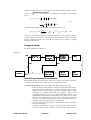
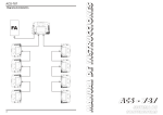
Program steps:
These are summarised in figure 4.3.
Figure 4.3
EHJLQ
!
VHOHFW HIIHFWLYH
HPLV FRHIIW
!
ILOH
UHDG DQG YHULI\
HIIHFWLYH HPLV
!
FRHIIW ILOH
HQWHU ILW FKRLFHV
VHOHFW [VHFW
VSHFLI\ RXWSXW
HQHUJLHV
DQG SODVPD
SDUDPHWHUV
UHSHDW
!
!
UHSHDW
2XWSXW WDEOHV
DQG JUDSKV
HQG
GLVSOD\ FKDUJH
H[FKDQJH FURVV
VHFWLRQ JUDSK
FRPSXWH FXELF
LQWHUSRODWH WR
VSOLQH DQG
SODVPD
PLQLPD[ ILW
FRQGLWLRQV
Interactive parameter comments:
Most ADAS interactive routines have three tasks, namely, file selection, user data
processing and output . This is achieved in three sequential windows.
The file selection window appears first and has the appearance shown below.
1. Data root shows the full pathway to the appropriate data subdirectories.
Click the Central Data button to insert the default central ADAS
pathway to the correct data type. Note that each type of data is stored
according to its ADAS data format (adf number). adf12 is the
appropriate format for use by the program ADAS303. Details of the
organisation of such data is given in the appxa-12. Click the User Data
button to insert the pathway to your own data. Note that your data must
be held in a similar file structure to central ADAS, but with your
identifier replacing the first adas, to use this facility.
2. The Data root can be edited directly. Click the Edit Path Name button
first to permit editing
3. Available sub-directories are shown in the large file display window.
There are a large number of these. They are stored in sub-directories
ADAS User manual
Chap4-03
17 March 2003
4.
5.
6.
by donor which is usually neutral but not necessarily so (eg. qef93#h).
The individual members are identified by the subdirectory name, a code
and then fully ionised receiver (eg. qef93#h_be4.dat). The data sets
generally contain many individual spectrum lines. Scroll bars appear if
the number of entries exceed the file display window size. Such data is
generally stored by year number (eg. 93 ) with the most recent data to
be preferred. Click on a name to select it. The selected name appears
in the smaller selection window above the file display window. Then
its sub-directories in turn are displayed in the file display window.
Ultimately the individual datafiles are presented for selection. Datafiles
all have the termination .dat.
Once a data file is selected, the set of buttons at the bottom of the main
window become active.
Clicking on the Browse Comments button displays any information
stored with the selected datafile. It is important to use this facility to
find out what is broadly available in the dataset. The possibility of
browsing the comments appears in the subsequent main window also.
Clicking the Done button moves you forward to the next window.
Clicking the Cancel button takes you back to the previous window
1
2
3
4
6
5
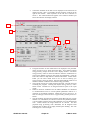
The processing options window is shown below:
1. An arbitrary title may be given for the case being processed. For
information the full pathway to the dataset being analysed is also
shown. The button Browse comments again allows display of the
information field section at the foot of the selected dataset, if it exists.
2. The output data extracted from the datafile may be fitted with a
polynomial. Clicking the Fit Polynomial button activates this. The
accuracy of the fitting required may be specified in the editable box.
The value in the box is editable only if the Fit Polynomial button is
active.
ADAS User manual
Chap4-03
17 March 2003
3.
Transitions available in the data set are displayed in the transition list
display window. This is a scrollable window using the scroll bar to the
right of the window. Click anywhere on the row for a transition to
select it. The selected transition appears in the selection window just
above the transition list display window.
1
2
3
7
6
4
5
4.
5.
6.
7.
ADAS User manual
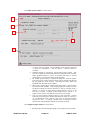
Energies/velocities for the neutral donor are displayed. The particular
choice of units in use is shown below the table. Your settings of beam
energy/velocity (output) are shown in the display window. The beam
energy/velocity values at which the effective emission coefficients are
stored in the datafile (input) are also shown for information. Click the
Edit Table button to drop-down the ADAS Table Editor. Within Table
Editor you can select which units to use as well as entering you
energy/velocity values for output. Note that final graphed results are of
effective emission coefficient versus beam energy (eV/amu).
The program recovers the output energies/velocities you used when last
executing the program. Pressing the Default Energy/Velocity values
button inserts a default set of energies/velocities equal to the input
values
Effective emission coefficients for the ADF12 database are calculated
at one-dimensional scans in various plasma parameters relative to a
reference set of plasma conditions. Details are given in appxa-12. To
alter the settings, activate the Select supplementary plasma parameters
button.
The sub-windows become active with the output data entry box in each
editable. For information, the reference value of each plasma parameter
is given together with the range of the parameter in its one-dimensional
scan. Values outside the range should not be entered. For data
prepared using processing code ADAS309, the B magnetic field
parameter has no effect, but is simply used for place holding. The scan
in B Magnetic is of zero length.
Chap4-03
17 March 2003
The output options window is shown below
1
2
3
4
5
1.
2.
3.
4.
5.
As in the previous window, the full pathway to the file being analysed
is shown for information. Also the Browse comments button is
available.
Graphical display is activated by the Graphical Output button. This
will cause a graph to be displayed following completion of this window.
When graphical display is active, an arbitrary title may be entered
which appears on the top line of the displayed graph.
By default, graph scaling is adjusted to match the required outputs.
Press the Explicit Scaling button to allow explicit minima and maxima
for the graph axes to be inserted. Activating this button makes the
minimum and maximum boxes editable.
Hard copy is activated by the Enable Hard Copy button. The File name
box then becomes editable. If the output graphic file already exits and
the Replace button has not been activated, a ‘pop-up’ window issues a
warning. A choice of output graph plotting devices is given in the
Device list window. Clicking on the required device selects it. It
appears in the selection window above the Device list window.
The Text Output button activates writing to a text output file. The file
name may be entered in the editable File name box when Text Output is
on. The default file name ‘paper.txt’ may be set by pressing the button
Default file name. A ‘pop-up’ window issues a warning if the file
already exists and the Replace button has not been activated.
The Graphical output window is shown below
1. Printing of the currently displayed graph is activated by the Print button.
ADAS User manual
Chap4-03
17 March 2003
1
Illustration:
Figure 4.3
ADAS User manual
Chap4-03
17 March 2003
Table 4.3
ADAS RELEASE: ADAS98 V2.5.6 PROGRAM: ADAS303 V1.10 DATE: 24/11/02 TIME: 10:35
******* TABULAR OUTPUT FROM EFF. EMISSION COEFFTS. INTERROGATION PROGRAM: ADAS303 - DATE: 24/11/02 *******
------------------ADAS User manual example
------------------EFFECTIVE EMISSION COEFFICIENTS AS A FUNCTION OF NEUTRAL BEAM ENERGY
----------------------------------------------------------------------------DATA GENERATED USING PROGRAM: ADAS303
------------------------------------/packages/adas/adas/adf12/qef93#h/q - DATA-BLOCK: 5
EMITTING ION INFORMATION:
------------------------TRANSITION (N-N')
=
9-8
NEUTRAL ATOM DONOR
= H(1S)
BARE NUCLEUS RECEIVER
=
N+7
QCX SOURCE FILE MEMBER
= OLD#N7
PROCESSING CODE
= ADAS309
EMISSION TYPE
= CX
ONE DIMENSIONAL SCAN POSITIONS:
------------------------------INTERPOLATED
VALUES
PARAMETER
ION DENSITY (cm-3)
ION TEMPERATURE (eV)
Z-EFFECTIVE
MAGNETIC FIELD (T)
=
=
=
=
2.500D+13
5.000D+03
2.000D+00
3.000D+00
REFERENCE
VALUES
2.500D+13
5.000D+03
2.000D+00
3.000D+00
----------- BEAM ENERGY ----------EFFECTIVE
EV/AMU
AT. V0
CM/SEC
EMIS. COEF. (CM3/SEC)
1.000D+03
2.001D-01
4.377D+07
2.960D-12
1.500D+03
2.450D-01
5.361D+07
7.570D-12
2.000D+03
2.829D-01
6.190D+07
1.370D-11
3.000D+03
3.465D-01
7.581D+07
2.500D-11
5.000D+03
4.474D-01
9.787D+07
4.460D-11
7.000D+03
5.293D-01
1.158D+08
7.450D-11
1.000D+04
6.327D-01
1.384D+08
1.570D-10
1.500D+04
7.749D-01
1.695D+08
5.020D-10
2.000D+04
8.947D-01
1.957D+08
1.360D-09
3.000D+04
1.096D+00
2.397D+08
5.140D-09
4.000D+04
1.265D+00
2.768D+08
1.040D-08
5.000D+04
1.415D+00
3.095D+08
1.440D-08
6.000D+04
1.550D+00
3.390D+08
1.670D-08
7.000D+04
1.674D+00
3.662D+08
1.590D-08
8.000D+04
1.789D+00
3.915D+08
1.410D-08
1.000D+05
2.001D+00
4.377D+08
8.780D-09
1.500D+05
2.450D+00
5.361D+08
3.340D-09
2.000D+05
2.829D+00
6.190D+08
1.510D-09
3.000D+05
3.465D+00
7.581D+08
4.320D-10
------------------------------------------------------------------------------NOTE: * => EFF. EMISSION COEFFTS. EXTRAPOLATED FOR BEAM ENERGY VALUE
------------------------------------------------------------------------------ADAS RELEASE: ADAS98 V2.5.6 PROGRAM: ADAS303 V1.10 DATE: 24/11/02 TIME: 10:35
MINIMAX POLYNOMIAL FIT TO BEAM ENERGIES - TAYLOR COEFFICIENTS:
------------------------------------------------------------------------------- LOG10(EFF. EMISSION COEFFT.) versus LOG10(BEAM ENERGY<EV/AMU>) ------------------------------------------------------------------------------A( 1) = -5.380300525D+04
A( 2) =
1.096882509D+05
A( 3) = -9.720797664D+04
A( 4) =
4.887682803D+04
A( 5) = -1.524382089D+04
A( 6) =
3.018703409D+03
A( 7) = -3.705648601D+02
A( 8) =
2.577690218D+01
A( 9) = -7.778688441D-01
LOGFIT - DEGREE= 8 ACCURACY= 3.72% END GRADIENT: LOWER=
3.34 UPPER= -4.09
-------------------------------------------------------------------------------
Notes:
ADAS User manual
Chap4-03
17 March 2003