Download — User`s Manual —

System Analysis Total Environment for Laboratory
— Language and InTeractive Execution
Biological and Physiological Engineering Laboratory
Department of Information and Computer Sciences
Toyohashi University of Technology, Toyohashi 441–8580, JAPAN
— User’s Manual —
Contents
1 What is SATELLITE?
1.1 Concept of SATELLITE
1.2 SATELLITE Modules .
1.3 Platform Support . . . .
1.4 Examples . . . . . . . .
.
.
.
.
.
.
.
.
.
.
.
.
.
.
.
.
.
.
.
.
.
.
.
.
.
.
.
.
.
.
.
.
.
.
.
.
.
.
.
.
.
.
.
.
.
.
.
.
.
.
.
.
.
.
.
.
.
.
.
.
.
.
.
.
.
.
.
.
.
.
.
.
.
.
.
.
.
.
.
.
2 SATELLITE Shell and its functions
2.1 Introduction . . . . . . . . . . . . . . . . . . . . . . . . . . .
2.2 How to start SATELLITE . . . . . . . . . . . . . . . . . . .
2.3 Operation . . . . . . . . . . . . . . . . . . . . . . . . . . . .
2.3.1 Prompts and a window title . . . . . . . . . . . . . .
2.3.2 Editing . . . . . . . . . . . . . . . . . . . . . . . . .
2.3.3 Preprocessor . . . . . . . . . . . . . . . . . . . . . .
2.3.4 Arithmetical operation . . . . . . . . . . . . . . . . .
2.4 Data handling . . . . . . . . . . . . . . . . . . . . . . . . . .
2.4.1 Objects and classes . . . . . . . . . . . . . . . . . . .
2.4.2 Class definition . . . . . . . . . . . . . . . . . . . . .
2.4.3 Conversions between two or more object classes . . .
2.4.4 Type of object . . . . . . . . . . . . . . . . . . . . .
2.5 Expressions and operators . . . . . . . . . . . . . . . . . . .
2.6 Internal constants . . . . . . . . . . . . . . . . . . . . . . .
2.7 Control sequence . . . . . . . . . . . . . . . . . . . . . . . .
2.7.1 IF sequence . . . . . . . . . . . . . . . . . . . . . . .
2.7.2 WHILE and DO-WHILE sequences . . . . . . . . .
2.7.3 FOR sequence . . . . . . . . . . . . . . . . . . . . .
2.8 Functions and procedures . . . . . . . . . . . . . . . . . . .
2.8.1 The scope of variables and constants, and arguments
2.8.2 Internal functions . . . . . . . . . . . . . . . . . . . .
2.8.3 User-defined function . . . . . . . . . . . . . . . . .
2.8.4 Input and output . . . . . . . . . . . . . . . . . . . .
2.8.5 Data stream handling . . . . . . . . . . . . . . . . .
2.9 Programming . . . . . . . . . . . . . . . . . . . . . . . . . .
2.9.1 Online message . . . . . . . . . . . . . . . . . . . . .
2.9.2 Loading a program from a file . . . . . . . . . . . . .
.
.
.
.
.
.
.
.
.
.
.
.
.
.
.
.
.
.
.
.
.
.
.
.
. . . . . . .
. . . . . . .
. . . . . . .
. . . . . . .
. . . . . . .
. . . . . . .
. . . . . . .
. . . . . . .
. . . . . . .
. . . . . . .
. . . . . . .
. . . . . . .
. . . . . . .
. . . . . . .
. . . . . . .
. . . . . . .
. . . . . . .
. . . . . . .
. . . . . . .
in functions
. . . . . . .
. . . . . . .
. . . . . . .
. . . . . . .
. . . . . . .
. . . . . . .
. . . . . . .
3 SYSTEM Module — SYSTEM
3.1 HELP — displaying a command manual . . . . . . . . . . . . .
3.2 HEADER — displaying or modifying the header information of
3.3 WAIT — interrupting the execution of a program . . . . . . . .
3.4 REFORM — changing the size or index of data . . . . . . . . .
3.5 BM — data monitoring . . . . . . . . . . . . . . . . . . . . . .
3.6 SAM — sampling frequency setting . . . . . . . . . . . . . . . .
3.7 CUT — selecting a subset of data . . . . . . . . . . . . . . . .
i
.
.
.
.
.
a
.
.
.
.
.
. . .
data
. . .
. . .
. . .
. . .
. . .
.
.
.
.
.
.
.
.
1
1
2
4
5
. . . . . . . . .
. . . . . . . . .
. . . . . . . . .
. . . . . . . . .
. . . . . . . . .
. . . . . . . . .
. . . . . . . . .
. . . . . . . . .
. . . . . . . . .
. . . . . . . . .
. . . . . . . . .
. . . . . . . . .
. . . . . . . . .
. . . . . . . . .
. . . . . . . . .
. . . . . . . . .
. . . . . . . . .
. . . . . . . . .
. . . . . . . . .
and procedures
. . . . . . . . .
. . . . . . . . .
. . . . . . . . .
. . . . . . . . .
. . . . . . . . .
. . . . . . . . .
. . . . . . . . .
.
.
.
.
.
.
.
.
.
.
.
.
.
.
.
.
.
.
.
.
.
.
.
.
.
.
.
8
8
8
10
10
11
14
14
14
14
20
20
21
21
22
23
23
24
25
25
25
26
27
29
30
31
31
31
.
.
.
.
.
.
.
33
33
33
33
34
35
35
36
.
.
.
.
. .
file
. .
. .
. .
. .
. .
.
.
.
.
.
.
.
.
.
.
.
.
.
.
.
.
.
.
.
.
.
.
.
.
.
.
.
.
.
.
.
.
.
.
.
.
.
.
.
.
.
.
.
.
.
.
.
.
.
.
.
.
.
.
.
.
.
.
.
.
.
.
.
.
.
.
.
.
.
.
.
.
.
.
.
.
.
.
.
.
.
.
.
.
ii
CONTENTS
3.8
3.9
3.10
3.11
3.12
3.13
3.14
3.15
3.16
3.17
3.18
PUT — replacing old data with new one . . . . . . . . . . .
MERGE — merging two data sets . . . . . . . . . . . . . .
FILL — filling data with a specified value . . . . . . . . . .
ZERO — filling data with 0 . . . . . . . . . . . . . . . . . .
REVERSE — reversing the order of data . . . . . . . . . .
ROTATE — rotating data . . . . . . . . . . . . . . . . . . .
MABI — selecting the subsequence of data . . . . . . . . .
GET — getting a value at the specified position of data . .
MAXPOS — getting the position of the maximum in data .
MAX — getting the maximum of data . . . . . . . . . . . .
FIND — finding the value close to the specified one in data
.
.
.
.
.
.
.
.
.
.
.
.
.
.
.
.
.
.
.
.
.
.
.
.
.
.
.
.
.
.
.
.
.
.
.
.
.
.
.
.
.
.
.
.
.
.
.
.
.
.
.
.
.
.
.
.
.
.
.
.
.
.
.
.
.
.
.
.
.
.
.
.
.
.
.
.
.
.
.
.
.
.
.
.
.
.
.
.
.
.
.
.
.
.
.
.
.
.
.
.
.
.
.
.
.
.
.
.
.
.
.
.
.
.
.
.
.
.
.
.
.
.
.
.
.
.
.
.
.
.
.
.
.
.
.
.
.
.
.
.
.
.
.
.
.
.
.
.
.
.
.
.
.
.
.
.
.
.
.
.
.
.
.
.
.
.
.
.
.
.
.
.
.
.
.
.
.
.
.
.
.
.
.
.
.
.
.
38
39
40
40
41
43
44
45
46
47
48
4 Interactive Signal Processing Package — ISPP
4.1 The command system of ISPP . . . . . . . . . .
4.2 Examples to use . . . . . . . . . . . . . . . . . .
4.2.1 Fourier transform . . . . . . . . . . . . . .
4.2.2 Filtering . . . . . . . . . . . . . . . . . . .
4.2.3 Matrix operation . . . . . . . . . . . . . .
.
.
.
.
.
.
.
.
.
.
.
.
.
.
.
.
.
.
.
.
.
.
.
.
.
.
.
.
.
.
.
.
.
.
.
.
.
.
.
.
.
.
.
.
.
.
.
.
.
.
.
.
.
.
.
.
.
.
.
.
.
.
.
.
.
.
.
.
.
.
.
.
.
.
.
.
.
.
.
.
.
.
.
.
.
.
.
.
.
.
.
.
.
.
.
.
.
.
.
.
.
.
.
.
.
.
.
.
.
.
.
.
.
.
.
50
50
50
50
57
63
5 Graphic Package Module — GPM
5.1 Introduction . . . . . . . . . . . . . . . .
5.2 Drawing and Printing . . . . . . . . . .
5.3 Examples . . . . . . . . . . . . . . . . .
5.3.1 Displaying 1-dimensional objects
5.3.2 Displaying 2-dimensional objects
.
.
.
.
.
.
.
.
.
.
.
.
.
.
.
.
.
.
.
.
.
.
.
.
.
.
.
.
.
.
.
.
.
.
.
.
.
.
.
.
.
.
.
.
.
.
.
.
.
.
.
.
.
.
.
.
.
.
.
.
.
.
.
.
.
.
.
.
.
.
.
.
.
.
.
.
.
.
.
.
.
.
.
.
.
.
.
.
.
.
.
.
.
.
.
.
.
.
.
.
.
.
.
.
.
.
.
.
.
.
.
.
.
.
.
65
65
65
67
67
70
6 Back-Propagation Simulator — BPS
6.1 Introduction . . . . . . . . . . . . . . . . . . . . . . . . . . . .
6.2 The file types used in BPS . . . . . . . . . . . . . . . . . . . .
6.3 BPS use example . . . . . . . . . . . . . . . . . . . . . . . . .
6.3.1 Preparation of “input”, “teach”, and “test” data files
6.3.2 Setting learning parameters . . . . . . . . . . . . . . .
6.3.3 Initialization of weights . . . . . . . . . . . . . . . . .
6.3.4 Learning . . . . . . . . . . . . . . . . . . . . . . . . . .
6.3.5 MLP testing . . . . . . . . . . . . . . . . . . . . . . .
6.3.6 Tracing connection weights and errors . . . . . . . . .
6.3.7 Internal representation analysis of MLP . . . . . . . .
.
.
.
.
.
.
.
.
.
.
.
.
.
.
.
.
.
.
.
.
.
.
.
.
.
.
.
.
.
.
.
.
.
.
.
.
.
.
.
.
.
.
.
.
.
.
.
.
.
.
.
.
.
.
.
.
.
.
.
.
.
.
.
.
.
.
.
.
.
.
.
.
.
.
.
.
.
.
.
.
.
.
.
.
.
.
.
.
.
.
.
.
.
.
.
.
.
.
.
.
.
.
.
.
.
.
.
.
.
.
.
.
.
.
.
.
.
.
.
.
.
.
.
.
.
.
.
.
.
.
.
.
.
.
.
.
.
.
.
.
.
.
.
.
.
.
.
.
.
.
.
.
.
.
.
.
.
.
.
.
72
72
72
72
73
74
77
79
81
82
83
7 Neural Circuit Simulator — NCS
7.1 Introduction . . . . . . . . . . . . . . . . . . . . . . . . . . . . . . .
7.1.1 Basic specifications . . . . . . . . . . . . . . . . . . . . . . .
7.1.2 Concept of modularization . . . . . . . . . . . . . . . . . .
7.2 NCS Language . . . . . . . . . . . . . . . . . . . . . . . . . . . . .
7.2.1 Reserved words . . . . . . . . . . . . . . . . . . . . . . . . .
7.2.2 Library functions . . . . . . . . . . . . . . . . . . . . . . . .
7.2.3 Description of modules . . . . . . . . . . . . . . . . . . . . .
7.2.4 Example — Hodgkin-Huxley model . . . . . . . . . . . . .
7.3 How to use NCS . . . . . . . . . . . . . . . . . . . . . . . . . . . .
7.3.1 Preparation of a model file . . . . . . . . . . . . . . . . . .
7.3.2 Registration of a model file . . . . . . . . . . . . . . . . . .
7.3.3 Preparation of an execution and a simulation condition file
7.3.4 Setting simulation conditions . . . . . . . . . . . . . . . . .
7.3.5 Execution of simulation . . . . . . . . . . . . . . . . . . . .
7.3.6 Use of batch file . . . . . . . . . . . . . . . . . . . . . . . .
7.3.7 Display and analysis of simulation results . . . . . . . . . .
.
.
.
.
.
.
.
.
.
.
.
.
.
.
.
.
.
.
.
.
.
.
.
.
.
.
.
.
.
.
.
.
.
.
.
.
.
.
.
.
.
.
.
.
.
.
.
.
.
.
.
.
.
.
.
.
.
.
.
.
.
.
.
.
.
.
.
.
.
.
.
.
.
.
.
.
.
.
.
.
.
.
.
.
.
.
.
.
.
.
.
.
.
.
.
.
.
.
.
.
.
.
.
.
.
.
.
.
.
.
.
.
.
.
.
.
.
.
.
.
.
.
.
.
.
.
.
.
.
.
.
.
.
.
.
.
.
.
.
.
.
.
.
.
.
.
.
.
.
.
.
.
.
.
.
.
.
.
.
.
.
.
.
.
.
.
.
.
.
.
.
.
.
.
.
.
.
.
.
.
.
.
.
.
.
.
.
.
.
.
.
.
.
.
.
.
.
.
.
.
.
.
.
.
.
.
.
.
85
85
85
85
88
89
89
92
100
104
104
104
105
105
110
110
111
.
.
.
.
.
.
.
.
.
.
.
.
.
.
.
.
.
.
.
.
.
.
.
.
.
Chapter 1
What is SATELLITE?
1.1
Concept of SATELLITE
It is generally agreed that the biological system is one of the most complex and sophisticated mechanisms
on earth. However, in this moment, since there are few systematic theories for approaching such systems,
trial and error studies based on knowledge of physiology, psychology, etc., has to continue. Environment
to support and realize the ideas of scientists could be so important to advance the research. We assert
that the establishment of basic platform for data analysis and model simulation could be relevant for
analyzing the complex systems such as neural systems.
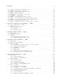
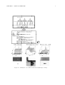
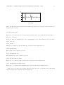
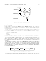
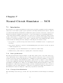
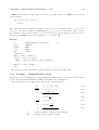
The basic concept of system analysis forms the cycle: data analysis, modeling, computer simulation,
evaluation and experimental testing, as shown in Figure 1.1. SATELLITE (System Analysis Total
Environment for Laboratory — Language and InTeractive Execution) has been developed considering
this scheme.
ISPP
measurement
NCS
Signal
Processing
NPE
Modeling
Parameter Estimation
BPS
Simulation
Evaluation
GPM
Figure 1.1: A general flow chart of biological system analysis.
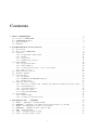
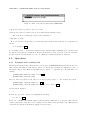
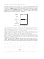
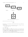
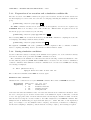
SATELLITE consists of the SATELLITE-shell which provides interactive and C-like language processing system, and several modules which together cover more than 200 commands and (signal processing,
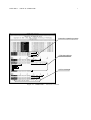
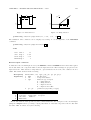
numerical simulation, etc. See also Figure 1.2). The most important facility of SATELLITE-shell is an
interactive operating environment. User can execute command sequence from the text file (batch processing) in case of the complex and large scale simulations (see also Figure 1.3). One can also visualize
data and print it.
1
2
CHAPTER 1. WHAT IS SATELLITE?
Program
(Analysis Algorithm)
Execute
Extensity
Interpreter
Objects
built-in functions
operators
Functions
Procedures
data
Interface
Protocol
External Functions
ISPP
Digital signal
processing
GPM
drawing & reporting
SL-UTIL
NCS
Utilities
Ionic current model
simulation
BPS
NPE
Neural network
simulation
Nonlinear parameter
estimation
Application
Softwares
Figure 1.2: A modular scheme of SATELLITE system.
1.2
SATELLITE Modules
SATELLITE organizes analysis techniques for various systems by grouping its functions into modules,
according to the purpose or method. There are several modules containing basic tools for system analysis,
such as digital signal processing, numerical simulation, model parameter estimation, etc., as listed below.
Details are described in the subsequent chapters.
SYSTEM module is a gathering of basic functions for handling data. It includes the functions such
as picking up data, finding a maximum or minimum of a sequence, modifying data format, displaying
header information of data files, etc.
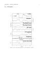
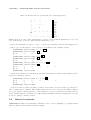
ISPP (Interactive Signal Processing Package) is a module for data analysis based on signal
processing and statistical theories. They are extremely important for modeling and extracting the characteristics from experimental data. Built-in commands can be applied to not only the time series, but
also the multi-dimensional data (see also Figure 1.4).
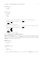
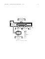
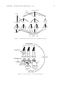
NCS (Neural Circuit Simulator) is a neural modeling and simulation environment. In this system,
special description language is utilized to describe the neuronal properties and the network structure.
This language offers an environment in which the large scale physiological model can be described easily
in NCS (see also Figure 1.5).
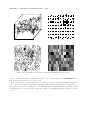
BPS (Back-Propagation Simulator) is developed to examine neural network characteristics and
capabilities. Function for tracing weight change offers precious data for analysis of learning process, local
minima, and internal network representation (see also Figure 1.6).
3
CHAPTER 1. WHAT IS SATELLITE?
interactive operating system
C like descriptions
on-line message
Figure 1.3: SATELLITE — interactive terminal.
CHAPTER 1. WHAT IS SATELLITE?
4
GPM (Graphic Package Module) From the standpoint of data analysis, visualization of data is
much more important than numerical evaluation. GPM module provides various graphic functions for
making charts, contour maps, bird’s-eye pictures, etc. The images can also be printed.
1.3
Platform Support
SATELLITE runs on the following platforms:
Operating system
Window system
Language to code
:
:
:
:
:
:
:
:
:
:
:
from SunOS 4.1.2
from Solaris 2.5
from HP-UX 9.05
from HP-UX 10.01
from DEC OSF/1 V3.0
from Digital UNIX V3.2c
from FreeBSD 2.1.0R
from Linux 2.0.0
from X Window Ver.11 R4
from OSF/Motif Ver.1.1
C Language
CHAPTER 1. WHAT IS SATELLITE?
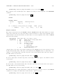
1.4
Examples
Figure 1.4: Biological signals during micro gravity (Example of ISPP).
5
CHAPTER 1. WHAT IS SATELLITE?
Figure 1.5: Simulation of a realistic neural etwork (Example of NCS).
6
CHAPTER 1. WHAT IS SATELLITE?
Figure 1.6: Simulation of artificial neural network (Example of BPS).
7
Chapter 2
SATELLITE Shell and its functions
2.1
Introduction
Signal processing techniques, simulations using mathematical models, etc., are effective for analysis of
the organizations and biological systems. Various software systems, such as Mathematica, LabVIEW
and AVS have been provided. However, if we use these software products, the whole efficiency may fall
remarkably because of data conversion to other systems.
SATELLITE enables to perform the consistent processing even if we use the completely different application software systems. It places simulators and signal processing packages as its external functions and
organizes them along with API (Application Program Interface) specification. The merit of SATELLITE
is that several different data sets, such as (multi-dimensional) time series, matrices, and so on, can be
processed to make analyzing the biological system easier.
The processing system of SATELLITE is an interpreter. Programs are translated into the intermediate
stack code. The stack machine code is executed by stack machines. Therefore, the repetition procedures
or functions, such as for command and while command, are performed at slightly higher speed. The
internal composition is shown as follows:
Simple line editor
↓
Preprocessor
↓
Lexical and syntax analysis
↓
Stack machine code
↓
Stack machine (execution)
If the program is syntactically correct, the processing system will translate it into the stack machine
code, and execute it. Frequently, one may want to use an editor, check a file name, change a current
directory, use UNIX commands, etc. If the token that appears at the beginning of a sentence is not
defined and is not substitution, SATELLITE passes such commands to Bourne shell of UNIX.
2.2
How to start SATELLITE
SATELLITE is started by typing “sl”, shown as follows:
8
CHAPTER 2. SATELLITE SHELL AND ITS FUNCTIONS
9
Figure 2.1: X-Window after starting SATELLITE
% sl ←where ←- stands for CR key. The X-Window after starting SATELLITE is shown in Figure 2.1.
Right after starting, the rc file (/usr/local/satellite/lib/satellite/rc.sl) which is prepared by the system
is automatically read at first, and the setup file (˜/.setup.sl) which is set by each user is read the next.
Since these files are processed in the state of “echo off”, messages of UNIX commands are not displayed
on a terminal, except the standard output errors. To display the messages, it is necessary to use the
standard output errors, or redirect the output as
echo "Welcome to SATELLITE WORLD" > /dev/tty
Fundamentally, we can write anything to the system rc file and the user setup file, as long as it is
syntactically correct. However, the starting will become slow if we call external executions frequently.
Generally we put the definitions of system modules in the system rc file, and the definitions of user
modules (commands), aliases, sampling frequency, the functions used often, and the variables used in the
user setup file.
This system is terminated by typing either “close”, “exit”, or Ctrl-D, shown as follows:
[]SATELLITE[]/home/tom:[1]% close ←[]SATELLITE[]/home/tom:[1]% exit ←[]SATELLITE[]/home/tom:[1]% ^D
Right after terminating, the user clean file ( /.clean.sl) is executed. Then the history is saved to the file
( /.history.sl), after execution of the closing commands of system modules, release of the system common
area (shared memory), destruction of system parameter area (temporary directory), dispatch of the end
signals to all child processes, etc., are performed.
The options for starting SATELLITE are as follows:
- read a program from a standard input (terminal)
-rc do not read the system rc file
-setup do not read the user setup file
-clean do not read the user clean file
CHAPTER 2. SATELLITE SHELL AND ITS FUNCTIONS
10
Figure 2.2: Title of the window while using SATELLITE
-log specify a directory name for the error log file
-work specify a directory name for the work domain (system parameter area)
The work directory (SLxxxx) is deleted after termination.
-temp same as -work
Moreover, if we have another file to read automatically besides the user setup file, we can specify it as
follows:
% sl setup2.sl ←Not providing option “-” means that reading from the standard input (terminal) is not performed and
the system closes right after termination. However, if the files are read, except the rc file, the setup file,
and the clean file, the system state is “echo on”. Then the command messages are displayed.
2.3
Operation
2.3.1
Prompts and a window title
The interpreter shows prompt. As shown below, the prompt of SATELLITE displays the current directory
name and the line number. Only last two parts of a current directory name are displayed because of
the length of the prompt. When a path name is not complete, “˜” appears before the path name. For
example,
[]SATELLITE[]/home/tom:[62]% cd work ←[]SATELLITE[]~tom/work:[63]%
Moreover, when a program exceeds 1 line, we are urged by the prompt “+”. For example, if we input
[]SATELLITE[]~tom/work:[63]% n = 0 ←[]SATELLITE[]~tom/work:[64]% for(i = 0; i < 10; i++) { ←the following is displayed:
+
In such case, process is completed by inputting the following:
n = n + 1 } ←In the case of X-Window terminal emulator (Xterm, Kterm, DECterm, etc.), the host name and the
complete path name of the directory are displayed at the window title (see Figure 2.2). That helps us
compensate the imperfect information displayed at the prompt.
11
CHAPTER 2. SATELLITE SHELL AND ITS FUNCTIONS
Table 2.1: Key binds of the line editor for SATELLITE
beginning of line
backward char
interrupt
delete char
end of file
listing up files
end of lines
forward char
backward delete char
newline
kill line
newline
down history
up history
tty start output
tty stop output
keyword completion
filename completion
command completion
2.3.2
ˆA
ˆB,
ˆC
ˆD,
ˆD
ˆD
ˆE
ˆF,
ˆH,
ˆJ
ˆK
ˆM
ˆN,
ˆP,
ˆQ
ˆS
ˆW
TAB,
TAB,
←
DEL
→
BS
↓
↑
ESC-ESC
ESC-ESC
Editing
The micro line editor for deletion or insertion of characters offers comfortable environment for interactive
programming from a terminal. This editor has internal buffers for editing. The contents in the buffers
are usually consistent with the character sequences which a user inputs, and displayed on the editing line
(back from the prompt).
Line editing
SATELLITE has a “GNU Emacs-like” micro line editor. The editing line is always in insert mode, and
we can move the cursor position by Ctrl-F (→), Ctrl-B (←), Ctrl-A, and Ctrl-E keys. Moreover, Ctrl-D
(DEL), Ctrl-H (BS), and Ctrl-K can perform deletion of characters. For example, when we input the
character sequence shown as follows:
[]SATELLITE[]~tom/rose:[63]% n = 0 ←the cursor is at the right-hand side of “0” now. By pressing Ctrl-H, “0” is eliminated and the cursor is
moved left. On the other hand, the cursor is moved left by Ctrl-B, without eliminating “0”. The cursor
moves to the head of the sentence, that is, to the position of “n”, by pressing Ctrl-A. The list of key
binds is shown in Table 2.1.
History
The inputs from a terminal are recorded in the history buffers. By pressing Ctrl-P, the history buffers
are traced back and the history is copied to the editing buffers. Ctrl-N performs the history search in
ascending order. We can freely edit and execute commands from the history buffers. For example,
CHAPTER 2. SATELLITE SHELL AND ITS FUNCTIONS
12
[]SATELLITE[]~tom/rose:[63]% n = 0 ←[]SATELLITE[]~tom/rose:[64]% j = 0 ←[]SATELLITE[]~tom/rose:[65]%
The following can be displayed by pressing Ctrl-P.
[]SATELLITE[]~tom/rose:[65]% ^P
[]SATELLITE[]~tom/rose:[64]% j = 0
Again, the following can be displayed by pressing Ctrl-P.
[]SATELLITE[]~tom/rose:[64]% j = 0 ^P
[]SATELLITE[]~tom/rose:[63]% n = 0
Moreover, the following can be displayed by pressing Ctrl-N.
[]SATELLITE[]~tom/rose:[63]% n = 0 ^N
[]SATELLITE[]~tom/rose:[64]% j = 0
When a character sequence is already in the editing buffer, only the history lines whose heads match
the character sequence are called. For example,
[]SATELLITE[]~tom/rose:[63]% n = 0 ←[]SATELLITE[]~tom/rose:[64]% j = 0 ←[]SATELLITE[]~tom/rose:[65]% n
By pressing Ctrl-P, the following is displayed:
[]SATELLITE[]~tom/rose:[65]% n ^P
[]SATELLITE[]~tom/rose:[63]% n = 0
Completion of file names and commands
If TAB key is pressed after inputting characters the help commands will be uniquely identified by the
head of the editing buffer. A command name will be completed and the full name will be displayed on
the terminal (and the editing buffer). The first candidate is shown if the command cannot be specified
uniquely. The next candidate is called by pressing TAB key again. For example, suppose that there are
six files in the current directory, namely, report1.tex, report2.tex, report3.tex, work1.tex, work2.tex, and
work3.tex. The file name or the directory name that starts with “wo” is searched and displayed from the
current directory, shown as follows:
[]SATELLITE[]~tom/rose:[88]% wo TAB
[]SATELLITE[]~tom/rose:[88]% work1.tex
The 2nd candidate is displayed by pressing TAB key again as follows:
[]SATELLITE[]~tom/rose:[88]% work1.tex TAB
[]SATELLITE[]~tom/rose:[88]% work2.tex
The candidates are searched in paths and order described by the environment variable PATH. If the
search cycle is completed, the editing buffer is cleared. After that, if TAB key is pressed again, the first
candidate will be called again. If there is no candidate, there is nothing to display.
CHAPTER 2. SATELLITE SHELL AND ITS FUNCTIONS
13
Completion of file names, UNIX commands, and directory names can be performed in the arbitrary
position of the editing buffer. The keywords for discrimination between both cases are the blank, just
before the cursor, the equaling character (=), and the character sequence divided by a double quotation
mark (”).
Reserved words or variable names in the symbol table of the interpreter can also be completed by
pressing Ctrl-W. For example, if we want to complete the reserved word or the variable name that starts
with “i”,
[]SATELLITE[]~tom/rose:[89]% i ^W
[]SATELLITE[]~tom/rose:[89]% if
By pressing Ctrl-W again, the 2nd candidate is displayed as follows:
[]SATELLITE[]~tom/rose:[89]% if ^W
[]SATELLITE[]~tom/rose:[89]% inline
Listing files
File names can be listed by Ctrl-D halfway. This function is helpful for checking the file names while
typing a program, or using UNIX commands such as cd, cp, mv, etc. For example,
[]SATELLITE[]~tom/rose:[8]% cd /home/tom/TeX/
As shown above, we can get the subdirectory names under /home/tom/Tex/ by pressing Ctrl-D, without
interrupting the input of character sequences.
[]SATELLITE[]~tom/rose:[8]% cd /home/tom/TeX/ ^D
RETINA1/
RETINA2/
work1.tex
work2.tex
[]SATELLITE[]~tom/rose:[8]% cd /home/tom/TeX/
Character “/” is appended to the end of directory names, “*” to executable file names, “@” to symbolic
links, “=” to sockets, “—” to FIFOs (pipe with a name), “%” to character devices, and “#” to block
devices, respectively. After displaying the list, the command inputted halfway is redisplayed.
We can also obtain the list of the files that start with certain characters. In the following example, all
of file and subdirectory names that start with “RE” will be displayed.
[]SATELLITE[]~tom/rose:[9]% cd /home/tom/TeX/RE ^D
/home/tom/TeX/RETINA1/ /home/tom/TeX/RETINA2/
[]SATELLITE[]~tom/rose:[9]% cd /home/tom/TeX/
In the special case, the list of all files and subdirectories which are consistent with the character sequences
including wild cards in the current directory can be displayed as follows:
[]SATELLITE[]~tom/rose:[10]%
where
^D
stands for a blank.
Calling UNIX commands
When the token not registered as reserved word or variable name appears in the head of the sentence,
the system leaves the processing to the UNIX shell. We can deal with UNIX commands in the same way
as the UNIX shell. When the variable with the same name as UNIX command is already registered, we
can avoid duplication by attaching the backslash (\) to the head of the commands.
CHAPTER 2. SATELLITE SHELL AND ITS FUNCTIONS
2.3.3
14
Preprocessor
The character sequence edited by the simple line editor is handed over to the preprocessor. It mainly
performs (1) history substitution, (2) alias substitution, and (3) parameter passing to SATELLITE
commands.
History substitution
!! refers to the last history items.
!str refers to the newest history item which starts with “str”.
In both cases the head of the sentence is recognized as a history item, and the replacement can be
performed without destroying the character sequences before and after it.
Alias substitution
If aliases are already defined, just the first token of the sentence is replaced. That is similar to the C
shell of UNIX.
Parameter passing
One of the strongest points of SATELLITE is that several parameters required in each function can be
passed interactively. The details are described in §2.9.1.
2.3.4
Arithmetical operation
To perform arithmetical operations using SATELLITE, we can input them directly. For example doing
multiplication 3 × 6,
[]SATELLITE[]~tom/rose:[13]% 3*6 ←18
[]SATELLITE[]~tom/rose:[14]%
Similarly dividing, as follows:
[]SATELLITE[]~tom/rose:[14]% 3/6 ←0.5
[]SATELLITE[]~tom/rose:[15]%
2.4
Data handling
2.4.1
Objects and classes
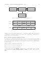
Data obtained from biological systems or numerical simulations is usually a multi-dimensional series. We
rarely pay attention to one value but rather deal with a set. SATELLITE deal with such a time series as
a single data class (object) and provides a data structure, namely “Series object”, which can treat the
differences between the temporal changes and the spatial changes of the multi-dimensional data efficiently
(see also Figure 2.3).
There are 4 other kinds of object classes than the Series class: Snapshot, String, Scalar, and File
classes. These classes are divided with respect to values they deal with (numerical values and character
15
CHAPTER 2. SATELLITE SHELL AND ITS FUNCTIONS
X:[60]
Time
2-dimensional Snapshot
100
X : 2-dimensional Series
60
0
Series
X[2][2]
File Object
Figure 2.3: Objects and their interrelationship
sequences). Scalar, Snapshot, Series, and File are objects expecting numerical values. The characteristics
of classes are inherited in the order of listing, taking Scalar as a super class. The Snapshot object is
a set of Scalar objects equivalent to the multi-dimensional arrangements for general-purpose languages.
The Series object can be viewed as a series of Snapshots in time, that is, 1-dimensional arrangement
of Snapshot objects. The File object requires a file name for handling the specified data on the UNIX
system.
Each object encapsulates data and processing methods. Arithmetical operations are different for
Scalar, Series, Snapshot, String, and File objects. In case of the Scalar object, the addition is performed
by adding up only 1-point data, as shown in Figure 2.4.
Figure 2.4: Addition between two Scalar objects
In case of the Series object, all values on the time-axis must be added simultaneously, as shown in Figure
2.5.
Time
Figure 2.5: Addition between two Series objects
5 kinds of object classes used in SATELLITE are explained in the pages that follow.
16
CHAPTER 2. SATELLITE SHELL AND ITS FUNCTIONS
7
6
6th
5
5th
4
4th
3
3rd
2
Time
2nd
1
1st
0th
Figure 2.6: Data organization in 1-dimensional Series object
Series object
Series is the object class in which a set of multi-dimensional data is lined to the direction of a time-axis
(Figure 2.3). The Series object that includes a single value is the same as 1-dimensional array in generalpurpose languages (Figure 2.6). The operation between two or more Series classes is possible only when
each size of a data set (Snapshot) is the same. That is, we cannot deal with a 2-dimensional Series object
and a 1-dimensional Series object together. Moreover, when the length of the direction of the time-axis
is different, the operation is performed within the limits of the shorter one, and the remainder is copied
as it is.
A mixed operation between a Series object and a Scalar object can be performed, e.g., the multiplication
of the Scalar object and each element in the Series objects. The characteristics of Series objects are the
implicit calculations repeated to each element and the operation functions for time series data by the
operators “[ ]” and “:[ ]”, such as selection, filling, etc.
Here, some examples of operations on Series objects are shown below. Data from 1 to 7 are stored in
a 1-dimensional Series object by the following command (see also Figure 2.6):
[]SATELLITE[]~tom/rose:[27]% x = 1~7 ←Here, ”˜” is the operator for generating an arithmetical series with a margin 1 (see §2.5 for further
details).
[]SATELLITE[]~tom/rose:[28]% x ←[0]:%
1
2
[5]:%
6
7
[]SATELLITE[]~tom/rose:[29]%
3
4
5
We can check the 3rd element as follows:
[]SATELLITE[]~tom/rose:[29]% x:[3] ←4
[]SATELLITE[]~tom/rose:[30]%
The next example shows the operation on a multi-dimensional object. The object class is defined as
follows (see §2.4.2 for further details):
[]SATELLITE[]~tom/rose:[30]% series y[2][2] ←A value of y[0][1] is assigned, e.g.,
[]SATELLITE[]~tom/rose:[31]% y[0][1] = x ←To display the value of y[0][1], type as follows (see also Figure 2.7):
[]SATELLITE[]~tom/rose:[32]% y[0][1] ←[0]:%
1
2
3
4
5
17
CHAPTER 2. SATELLITE SHELL AND ITS FUNCTIONS
7
6
5
4
6th
3
5th
2
4th
1
3rd
Time
2nd
1st
0th
7
6
5
4
3
2
1
Figure 2.7: Data organization in 2-dimensional Series object (Example 1)
7
6
5
6th
5th
4th
3rd
Time
2nd
1st
0th
4
4
3
2
1
Figure 2.8: Data organization in 2-dimensional Series object (Example 2)
[5]:%
6
7
[]SATELLITE[]~tom/rose:[33]%
To obtain the spatial data of certain time, type (see also Figure 2.8),
[]SATELLITE[] tom/rose:[33]% y:[3] ←[0][1]:%
0
4
[0][0]:%
0
0
[]SATELLITE[] tom/rose:[34]%
Snapshot object
Snapshot is the object class similar to matrix (Figure 2.3). It is for dealing with static data sets, and
used as a subset of a Series object or a matrix. Only on Snapshot objects with the same size can be
performed operations. For the mixed operation with a Scalar object, the same operation is repeatedly
performed between each element of the Snapshot and the Scalar.
Some examples of operations on Snapshot objects are shown below (Figure 2.9). First, an object class
is defined as follows (see §2.4.2 for further details):
[]SATELLITE[]~tom/rose:[34]%
[]SATELLITE[]~tom/rose:[35]%
[0][1]:%
0
[0][0]:%
0
[]SATELLITE[]~tom/rose:[36]%
snapshot z[2][2] ←z ←0
0
A value is assigned to the item of this object as follows:
[]SATELLITE[]~tom/rose:[37]% z[0][1] = 4 ←[]SATELLITE[]~tom/rose:[38]% z ←4
4
Figure 2.9: Data organization in 2-dimensional Snapshot object.
CHAPTER 2. SATELLITE SHELL AND ITS FUNCTIONS
18
Figure 2.10: A Scalar object.
[0][1]:%
0
4
[0][0]:%
0
0
[]SATELLITE[]~tom/rose:[39]%
We can get the value of certain item as follows:
[]SATELLITE[]~tom/rose:[39]% z[0][1] ←4
[]SATELLITE[]~tom/rose:[40]%
Scalar object
Scalar is the object class for numbers, such as variables to control sequences, elements in Series objects,
etc.(Figure 2.10). It is expressed as the double precision number.
[]SATELLITE[]~tom/rose:[41]% k = 0.8 ←[]SATELLITE[]~tom/rose:[42]% k ←0.8
[]SATELLITE[]~tom/rose:[43]%
File object
This class is used for saving data in a file on a hard disk. Data can be loaded from files and stored to
files. Therefore, we can deal with it as with other objects, without taking care of the format or the data
type. Moreover, mixed operations with the Series object are also possible.
The File object has almost the same structure as Series, and can store two or more sets of multidimensional data (Series, Snapshot) in the direction of the “Record” (see Figure 2.11). Record corresponds
to the time of the Series object, and has flexible length. Each data stored in a record must have the same
size. Moreover, since the number of dimensions and indexes of the File object depends on that of the
object stored in the first place, the object with the different number of dimensions and indexes is stored
after conversion.
Storing is performed by assigining a data element to File object. For example, y (a Series or Snapshot
object) is stored to the record 0 of data.dat.
[]SATELLITE[]~tom/rose:[26]% $"data.dat":[0] = y ←In case of loading data, we just type the name of a File object in an editing line. SATELLITE will
automatically treat it as the Series object. For example, data in the record 0 of data.dat is loaded to x:
[]SATELLITE[]~tom/rose:[27]% x = $"data.dat":[0] ←All records of data.dat can be loaded to y as follows:
[]SATELLITE[]~tom/rose:[28]% y = $"data.dat" ←Both x and y are Series objects, and their dimension and index numbers depend on data.dat. For example,
when 2-dimensional data is stored in a record, x is 2 dimensional Series object and y is 3-dimensional
one.
19
CHAPTER 2. SATELLITE SHELL AND ITS FUNCTIONS
File type
Data type
Header part
256byte
Data part
Record 0
Owner
Comment
Date
Dimension
Record 1
Index
Record n-1
Record n
Figure 2.11: Data file structure
String class
File names are basic and important information for managing data. They usually include the attributes
or “serial numbers” of data. The String object is used for labeling, e.g., in the case of drawing a chart,
outputting a message from a program, etc. The concatenation, deletion, repetition, and separation are
performed by sending operators “+”, “-”, “*”, and “/”, respectively. A character sequence should be
marked by double quotation marks (”).
For example, concatenating a character sequence with another one is performed as follows:
[]SATELLITE[]~tom/rose:[29]% "test" + ".dat" ←test.dat
[]SATELLITE[]~tom/rose:[30]%
Moreover, we use “-” to delete a character sequence.
[]SATELLITE[]~tom/rose:[30]% "test.dat" - ".dat" ←test
[]SATELLITE[]~tom/rose:[31]%
For repetition of a character sequence, “*” is used.
[]SATELLITE[]~tom/rose:[31]% "ABC" * 4 ←ABCABCABCABC
[]SATELLITE[]~tom/rose:[32]%
In order to separate a character sequence, “/” is used.
[]SATELLITE[]~tom/rose:[32]% "A,BC,D,EFG,H,IJK," / "," ←[0]% A
BC
D
EFG
H
[5]% IJK
[]SATELLITE[]~tom/rose:[33]%
where “[0]%” and “[5]%” represent the index of data for displaying two or more elements.
CHAPTER 2. SATELLITE SHELL AND ITS FUNCTIONS
2.4.2
20
Class definition
Class definition of variables in SATELLITE does not restrain the types permanently, but generates the
objects whose contents are flexible. Definition of Series objects, with no index specifies the 1-dimensional
time series:
[]SATELLITE[]~tom/rose:[35]% series x ←The Series object 64 × 64 is defined by as follows:
[]SATELLITE[]~tom/rose:[36]% series y[64][64] ←Definition of Snapshot objects is performed as follows:
[]SATELLITE[]~tom/rose:[37]% snapshot a[10], b[20][20] ←In the case of Snapshot, we cannot omit the size. Scalar objects are defined as follows:
[]SATELLITE[]~tom/rose:[38]% scalar i, j, k ←Scalar objects are not allowed to have the size, that is, each object deal with only one value. Finally,
definition of String objects is performed as follows:
[]SATELLITE[]~tom/rose:[39]% string str, mstr[10] ←It is possible for String objects to specify their size.
2.4.3
Conversions between two or more object classes
The object class (type) of variables in SATELLITE is determined at the time of substitution. It is
the same as the size of the class on the right side of the equality work. The above-mentioned definition
method is used only for receiving values as arguments of a function, assigning values to multi-dimensional
objects, etc. We do not need to define the class in the case where it is determined by the assignment as
follows:
[]SATELLITE[]~tom/rose:[50]% a = 1 ←We cannot use undefined variables for the arguments of functions or procedures. For example, FFTC in
the ISPP module is one of such commands;
[]SATELLITE[]~tom/rose:[51]% fftc(P,x,y,u,v) ←where P is a flag for specifying the calculation method, x and y are input series, and u and v are output
series of the FFTC command. In this case, u and v should be defined before calling FFTC function.
Conversion between two object classes is automatically performed. In this way, we can change an
object class to another one. In case of the operation between String and Scalar objects, for example, the
Scalar value is converted to a character sequence. The resulting class is String, e.g.,
[]SATELLITE[]~tom/rose:[52]% "test" + 3 ←test3
[]SATELLITE[]~tom/rose:[53]% "" + 3.1415926 ←3.14159
[]SATELLITE[]~tom/rose:[54]%
CHAPTER 2. SATELLITE SHELL AND ITS FUNCTIONS
21
The reason why the result of ”” + 3.1415926 becomes 3.14159 is due to round off for displaying. A
numerical value is obtained after changing String into Scalar as follows:
[]SATELLITE[]~tom/rose:[54]% 3 + "3.1415926" ←6.1415926
[]SATELLITE[]~tom/rose:[55]% 0 + "1.08e-2" ←0.0108
[]SATELLITE[]~tom/rose:[56]%
Similarly other object conversions can be performed, such as Series → String, String → Series, etc.
Conversion between more than two objects can be also performed.
2.4.4
Type of object
To obtain the object class of the variable whose class is unknown, the TYPEOF command is used.
Suppose that x is Series object and y is Snapshot object. Then we can get type of each class of these
variables by the following:
[]SATELLITE[]~tom/rose:[56]% typeof(x) ←series
[]SATELLITE[]~tom/rose:[57]% typeof(y) ←snapshot
[]SATELLITE[]~tom/rose:[58]%
In order to get the index of a object, we use the INDEX command. For example, if we define a series
object as
[]SATELLITE[]~tom/rose:[58]% a = 1~10 ←then the index of the object can be obtained by
[]SATELLITE[]~tom/rose:[59]% index(a) ←10
[]SATELLITE[]~tom/rose:[60]%
In case of multi-dimensional data, such as b[10][50], the information is displayed as follows:
[]SATELLITE[]~tom/rose:[60]% snapshot b[10][50] ←[]SATELLITE[]~tom/rose:[61]% index(b) ←[0]:%
10
50
[]SATELLITE[]~tom/rose:[62]%
2.5
Expressions and operators
Expression relates not only simple arithmetical operations but also substitutions, functions, etc. The
results of the evaluation of expressions are displayed automatically, except for substitutions. Although
the notation of operators of SATELLITE is different from its internal functions’ one, they are internally
treated equally. The operator and the internal function appeared in an expression is sent to the linked
object and the first argument object respectively, as a message. Therefore, even if two operators or
internal functions are the same, their performance may be different and depending on the object class.
Operators include arithmetical operators, relational operators, logical operators, increment and decrement
22
CHAPTER 2. SATELLITE SHELL AND ITS FUNCTIONS
Table 2.2: Priority table for operators (in order of the high priority).
()
[]
:[]
b
right
!
−
++ −−
left
e
left
∗
/
%
left
+
−
left
>
>=
<
<= == ! = left
&&
left
||
left
= + = − = ∗ = / = b = right
Notice: In the above table, “right” means that the operator is combined with the right-hand side object, and
“left” means that the operator is combined with the left-hand side object.
operators, the substitution operator “=”, the “˜” operator for generating a sequence with margin 1, the
operator “( )” for connecting two or more series, etc. Followings are the examples of usage:
[]SATELLITE[]~tom/rose:[56]%
[]SATELLITE[]~tom/rose:[57]%
[0]:%
-3
-2
[]SATELLITE[]~tom/rose:[58]%
[]SATELLITE[]~tom/rose:[59]%
[0]:%
1
2
[]SATELLITE[]~tom/rose:[60]%
[]SATELLITE[]~tom/rose:[61]%
[0]:%
-3
-2
[5]:%
2
3
[]SATELLITE[] tom/rose:[62]%
x = -3~-1 ←x ←-1
y = 1~3 ←y ←3
z = (x, 0, y) ←z ←-1
0
1
Operators are interpreted by following the priority shown in Table 2.5. The following example demonstrates for comparison operators.
[]SATELLITE[]~tom/rose:[63]% (z > 0) * z ←[0]:%
-0
-0
-0
0
[5]:%
2
3
[]SATELLITE[]~tom/rose:[64]%
1
Objects are destroyed after performing operations. If we want to keep the results of operations, we
have to assign them to variables. The variable mentioned here can be regarded as a simple container
for objects, without restricting the type of data. Therefore, even if object names are the same, there is
some possibility that their contents become different after substitution. Memory management of objects
is done by “garbage collecting” method.
2.6
Internal constants
SATELLITE has defined several internal constants in order to ease programming or operating internal
functions. There are three kinds of internal constants:
CHAPTER 2. SATELLITE SHELL AND ITS FUNCTIONS
23
• Floating point constants, such as 3.0, 1.0e−5, etc, and character sequence constants, such as “Welcome to SATELLITE World”.
• Mathematical constants
180/π : DEG = 57.2957...
The base of log : E = 2.7182...
Euler’s constant : GAMMA = 0.5772...
√
Golden ratio : PHI = ( 5 + 1)/2 = 1.6180...
π : PI = 3.1415...
• User-defined constants defined by the command CONST
For example,
[]SATELLITE[]~tom/rose:[56]% const Degree = PI/180 ←SATELLITE treats the internal constants and user-defined constants equally. Moreover, we can change
the internal constant to the user-defined one by the command CONST. CONST can deal with the
expression in which its right-hand side is a formula or an object like Series. It is evaluated right after it
is defined. The difference between variables and constants is just in permission of substituting objects.
2.7
Control sequence
As in C language, we can use IF, WHILE, DO-WHILE, For as control sequences, and { ... } for
grouping statements together.
• if ( expr1 ) stmt1
• if ( expr1 ) stmt1 else stmt2
• while ( expr1 ) stmt1
• do stmt1 while ( expr1 )
• for ( expr1 ; expr2 ; expr3 ) stmt1
expr1, expr2, and expr3 are general expressions including substitutions or functions. stmt1 and stmt2
are single statements. A set of statements in parentheses { ... } is also regarded as the single statement.
AND operator “&&”, OR operator “| |” , and other relation operators can be used in expressions. If the
result of evaluation of an expression is equal to zero, it is treated as “false”, or else “true”. In the case
where two or more results are obtained by a logical operation, such as a comparison between two Series
objects, if all of them are not equal to zero, it is regarded as “true”.
2.7.1
IF sequence
If the result of the conditional expression expr1 is “true”, the first statement stmt1 is performed. If the
condition expr1 is evaluated as “false”, the next statement stmt2 is executed, instead of stmt1.
CHAPTER 2. SATELLITE SHELL AND ITS FUNCTIONS
24
IF sequence(1):
if ( expr1 ) {
stmt1;
}
IF sequence(2):
if ( expr1 ) {
stmt1;
} else {
stmt2;
}
For example, processing of “If x is smaller than n, then add x to s” is described as follows:
[]SATELLITE[]~tom/rose:[86]% if (x < n) { ←+ s = s + x ←+ } ←[]SATELLITE[]~tom/rose:[87]%
Processing of “If x is smaller than n, then add x to s, or else subtract x from s” is described as follows:
[]SATELLITE[]~tom/rose:[87]% if (x < n) { ←+ s = s + x ←+ } else { ←+ s = s - x ←+ } ←[]SATELLITE[]~tom/rose:[88]%
2.7.2
WHILE and DO-WHILE sequences
WHILE and DO-WHILE sequences controll the loops. They perform the statement stmt1 repeatedly
until the condition expr1 is true. In case of WHILE sequence, the evaluation of expr1 is performed
before the execution of stmt1, including its effects. On the other hand, the statement in case of DOWHILE is processed after execution of stmt1.
WHILE sequence:
while ( expr1 ) {
stmt1;
}
DO-WHILE sequence:
do {
stmt1;
} while ( expr1 );
Processing of “While x is smaller than n, add x to s” is described by the WHILE sequence as follows:
CHAPTER 2. SATELLITE SHELL AND ITS FUNCTIONS
25
[]SATELLITE[]~tom/rose:[89]% while (x < n) { ←+ s = s + x ←+ n++ ←+ } ←[]SATELLITE[]~tom/rose:[90]%
The same example by the DO-WHILE sequence is as follows:
[]SATELLITE[]~tom/rose:[90]% do { ←+ s = s + x ←+ n++ ←+ } while (x < n) ←[]SATELLITE[]~tom/rose:[91]%
2.7.3
FOR sequence
In FOR sequence, the first expression expr1 is evaluated only once, that is, during the initialization of a
loop. FOR sequence is terminated if expr2 is false, which is evaluated before each iteration. Expression
expr3 is used for the re-initialization of a loop after repetition.
FOR sequence:
for( expr1; expr2; expr3 ) {
stmt1;
}
For example, processing of “Add x to s n times” is described by the FOR sequence as follows:
[]SATELLITE[]~tom/rose:[91]% for (i=1; i<=n; i++) { ←+ s = s + x ←+ } ←[]SATELLITE[]~tom/rose:[92]%
BRAKE forces termination of a loop. CONTINUE returns a loop to its starting point.
2.8
Functions and procedures
2.8.1
The scope of variables and constants, and arguments in functions and
procedures
The variables in SATELLITE are effective only in the function or the procedure where they are defined,
that is, it is not allowed to refer to those variables in another function or procedure. In order to compare
external variables in a function or a procedure, we need to use the reserved word EXTERNAL.
Internal constants and the constants are defined by CONST. They are available in functions or
procedures after their definitions. Although we can define constants in a function or a procedure locally,
they become effective after processing.
Since all arguments of the functions and procedures in SATELLITE are handed over as variables, the
results obtained by operations on arguments inside return to the root.
CHAPTER 2. SATELLITE SHELL AND ITS FUNCTIONS
2.8.2
26
Internal functions
SATELLITE has defined some internal functions for mathematical calculations or system management.
The mathematical function library apply to all objects. All internal functions have the same priority.
Mathematical and system functions are shown in the following list (cf. Command Reference Manual):
List of mathematical functions
abs(x) |x|
acos(x) cos−1 x
asin(x) sin−1 x
atan(x) tan−1 x
atan2(x,y) tan−1 x/y, same as atan(x/y)
cos(x) cos x
exp(x) ex
exp2(x) 2x
int(x) the integer part of x (rounding off decimal fractions)
mod(x,y) the remainder of x/y, same as x % y
log(x) loge x (a natural logarithm)
log2(x) log2 x
log10(x) log10 x
pow(x,y) xy , same as x^y
sgn(x) the sign of x
sin(x) sin x
sqrt(x)
√
x
tan(x) tan x
List of system functions
abort() Termination of a program by force
alias(x,y) Alias operation
history(x) History operation
index(x) Acquisition of an object’s index
inline(x) Execution of a program from a file
length(x) Acquisition of the number of data points / elements
CHAPTER 2. SATELLITE SHELL AND ITS FUNCTIONS
27
printf(x, ...) Indication of objects
read(x) Reading an object
strlen(x) Acquisition of the length of a character sequence
typeof(x) Acquisition of an object class
undef(x) Elimination of a variable
unix(x) Execution of UNIX command
write type() Specification of a file type for writing
GarCo() Garbage collection
Symbols() Indication of a variable name (in symbol table)
Note: x and y are the function arguments. “...” stands for the arguments in which the number of them
is variable.
2.8.3
User-defined function
We can define functions and procedures of our own. For example, the function plusten that performs
“Add 10 to the argument n” is given as follows:
[]SATELLITE[]~tom/rose:[57]% func plusten(n) { ←+ return n + 10 ←+ } ←[]SATELLITE[]~tom/rose:[58]%
The following is an example of calling this function:
[]SATELLITE[]~tom/rose:[58]% num = 8 ←[]SATELLITE[]~tom/rose:[59]% plusten(num) ←18
[]SATELLITE[]~tom/rose:[60]%
Moreover, functions can be called recursively. The function fac (for obtaining x!) is described as follows:
[]SATELLITE[]~tom/rose:[60]% func fac(x) { ←+ if (x <= 0) return 1 else return x * fac(x-1) ←+ } ←[]SATELLITE[]~tom/rose:[61]%
The next example is the procedure that performs “Substitute n for the argument x and n + 1 for the
argument y”. At first, we have to define x and y before calling the procedure, as mentioned in §2.4.3.
[]SATELLITE[]~tom/rose:[61]% scalar x, y ←[]SATELLITE[]~tom/rose:[62]% proc plusone(n, x, y) { ←+ x = n ←+ y = n + 1 ←+ } ←[]SATELLITE[]~tom/rose:[63]%
CHAPTER 2. SATELLITE SHELL AND ITS FUNCTIONS
28
The following is an example of calling this procedure:
[]SATELLITE[]~tom/rose:[62]% plusone(14, x, y) ←[]SATELLITE[]~tom/rose:[63]% x ←14
[]SATELLITE[]~tom/rose:[64]% y ←15
[]SATELLITE[]~tom/rose:[65]%
The variables used in a function and procedure are local ones. They are effective only in the function
or procedure unless EXTERNAL is used. In order to use global variables, it is required to define every
time in the function or the procedure. The following is the same operation as the above mentioned
example except for using EXTERNAL definition of x and y:
[]SATELLITE[]~tom/rose:[65]% proc subplusone(n) { ←+ external x, y ←+ x = n ←+ y = n + 1 ←+ } ←[]SATELLITE[]~tom/rose:[66]%
Another example follows:
[]SATELLITE[]~tom/rose:[66]%
+ external x, y ←+ subplusone(gn) ←+ z = x + y ←+ return z ←+ } ←[]SATELLITE[]~tom/rose:[67]%
[]SATELLITE[]~tom/rose:[68]%
9
[]SATELLITE[]~tom/rose:[69]%
4
[]SATELLITE[]~tom/rose:[70]%
5
[]SATELLITE[]~tom/rose:[71]%
0
[]SATELLITE[]~tom/rose:[72]%
func glplusone(gn) { ←-
scalar x, y, z ←glplusone(4) ←x ←y ←z ←-
Since functions never check their arguments classes, the ones having multi-defined operators and mathematical functions are performed exactly, regardless of the object class of arguments (multi-state functions)
except the class the operators cannot deal with. The example of a sigmoidal function is shown. At first,
it is defined as follows:
[]SATELLITE[]~tom/rose:[72]% func sig(t) { ←+ return 1/(1+exp(-t)) ←} ←[]SATELLITE[]~tom/rose:[73]%
29
CHAPTER 2. SATELLITE SHELL AND ITS FUNCTIONS
When the argument t is a Scalar object, the return value of the function is also the Scalar object.
[]SATELLITE[]~tom/rose:[73]% sig(0) ←0.5
[]SATELLITE[]~tom/rose:[74]%
In the case where t is a Series object, we have
[]SATELLITE[]~tom/rose:[74]% sig(-10~10) ←[ 0]:%
4.54e-05 0.0001234 0.0003354 0.0009111
[ 5]:%
0.006693
0.01799
0.04743
0.1192
[10]:%
0.5
0.7311
0.8808
0.9526
[15]:%
0.9933
0.9975
0.9991
0.9997
[20]:%
1
[]SATELLITE[]~tom/rose:[75]%
0.002473
0.2689
0.982
0.9999
Thus, the series from −10 to 10 obtained by the operator “˜” (21 data points) is handed over to sig( ).
The result is the Series object with 21 elements. We can easily make programs dealing with time series
using mathematical formulas only. In the above mentioned example, the result is obtained just as we
intended in cases where the argument is a Scalar, Snapshot, Series, or File object. If the argument t is a
String object, an error message is returned.
[]SATELLITE[]~tom/rose:[75]% sig("test") ←sl: string not supported method
[]SATELLITE[]~tom/rose:[76]%
2.8.4
Input and output
There are some external functions and commands for displaying objects. Using PRINT, we only have
to arrange the objects to display (separated by commas). In SATELLITE, the message is displayed on
line according to specific format, e.g.,
[]SATELLITE[]~tom/rose:[70]% x = 3 ←[]SATELLITE[]~tom/rose:[71]% print "x = ", x, "\n" ←x = 3
[]SATELLITE[]~tom/rose:[72]% print (1, 2, 3, 4, 5), "\n" ←[0]:%
1
2
3
4
5
[]SATELLITE[]~tom/rose:[73]%
The function PRINTF is also available, We can specify the precision of displayed elements. Although
the usage is similar to the printf function of C language, it is internally different.
[]SATELLITE[]~tom/rose:[73]%
[]SATELLITE[]~tom/rose:[74]%
x = 3
[]SATELLITE[]~tom/rose:[75]%
[0]:%
1.0000
2.0000
[]SATELLITE[]~tom/rose:[76]%
x = 3 ←printf("x = %d\n", x) ←printf("%9.4f\n",(1,2,3,4,5)) ←3.0000
4.0000
5.0000
The READ function reads an object from a terminal. It receives an object class as argument in
character format and converts it to the class. The return value is the read object. In case of the objects
that consist of two or more elements like Series, the elements are separated by commas. For example,
30
CHAPTER 2. SATELLITE SHELL AND ITS FUNCTIONS
[]SATELLITE[]~tom/rose:[77]% y = read(series) ←1,2,3,4,5,6,7,8
The numerical values are stored in y as follows:
[]SATELLITE[]~tom/rose:[78]% y ←[0]:%
1
2
[5]:%
6
7
[]SATELLITE[]~tom/rose:[79]%
2.8.5
3
8
4
5
Data stream handling
The redirection of data displayed on terminal to variables or UNIX commands can be performed by the
data stream handling in SATELLITE. It is similar to a pipe in UNIX. The function UNIX is used for
interfacing UNIX with SATELLITE. It hands over a UNIX command to the shell. In SATELLITE, the
input data is converted into the String object. Then it can be substituted to a variable. Data from the
standard output can also be handed over to an UNIX command using the “<<” operator.
The example of the collective operation for all files listed by the ls command of UNIX in a current
directory is shown as follows. Function UNIX is used:
[]SATELLITE[]~tom/rose:[79]% files = unix("ls *.dat") ←[]SATELLITE[]~tom/rose:[80]% files ←[0]%
fnama1.dat
fname2.dat
fname3.dat
[3]%
fname4.dat
fname5.dat
[]SATELLITE[]~tom/rose:[81]% for(i=0;i<length(files);i++){ ←+
(Operation of files[i])
+ } ←[]SATELLITE[]~tom/rose:[82]%
The following is the example in which the data generated in SATELLITE is stored into a text file.
[]SATELLITE[]~tom/rose:[82]% t = 2 * PI * 0~1024 / 1024 ←[]SATELLITE[]~tom/rose:[83]% unix("cat > data.txt")<<sin(t) ←The next example is the reverse operation, that is, from a text file to an object.
[]SATELLITE[]~tom/rose:[84]% s = unix("cat data.txt") ←The String object s is converted to the Series object t by the following:
[]SATELLITE[]~tom/rose:[85]%
[]SATELLITE[]~tom/rose:[86]%
[
0]:%
0.000
0.006
[
5]:%
0.030
0.036
(Omitted)
[1015]:%
-0.05
-0.04
[1020]:%
-0.02
-0.01
[]SATELLITE[]~tom/rose:[87]%
t = 0 + s ←t ←0.012
0.018
0.042
0.049
-0.04
-0.01
-0.03
-0.00
0.024
0.055
-0.03
-0.00
CHAPTER 2. SATELLITE SHELL AND ITS FUNCTIONS
2.9
Programming
2.9.1
Online message
31
One of the special features of SATELLITE is that it allows us to deal with parameters interactively while
displaying their explanation. The parameters are separated by comma. Here, the example is shown, e.g.,
for function GRAPH:
[]SATELLITE[]~tom/rose:[13]% graph ←[]SATELLITE[]~tom/rose:[13]% graph(x,
..... Y-AXIS DATA ( Object or T F D )
It is required to input the object of Y-axis. If we input “volt”, for example, the following is displayed:
[]SATELLITE[]~tom/rose:[13]% graph(volt ←[]SATELLITE[]~tom/rose:[13]% graph(volt,"T",
..... X-AXIS DATA ( Object or T F D )
Next, the object of X-axis follows. Messages are displayed for all input parameters. If a default parameter
is acceptable, we just press the CR key to move to the next parameter.
The syntax of every SATELLITE command is checked. However, preprocessor can compensate for
simple mistakes. Parameters can be edited freely since they are stored in editting buffers.
2.9.2
Loading a program from a file
To make the interpreter load a program from a file, the function INLINE is used. Its argument is the file
name (it treats the file as the standard input). Each line of the program is processed one after another,
similarly as in the case of the input from a terminal. It is also possible to process the program of another
file from the one called. In fact, the INLINE is also processed in a syntactic mode and connects the
standard input of the interpreter to the file. The limitation is given by the number of files that can be
opened. If an error occurs while loading a file, the subsequent lines are not executed. The example of a
program file with name testsum.sl is shown as follows:
psum = 0;
for( i = 1; i <= 10; i++ ) {
sum = sum + i;
}
printf("sum = %d\n", sum);
Using INLINE the interpreter reads the above file.
[]SATELLITE[]~tom/rose:[14]% inline("testsum.sl") ←sum = 55
[]SATELLITE[]~tom/rose:[15]%
When required to read a file in another file, use INLINE in the file as follows:
sum = 0;
for( i = 1; i <= 10; i++ ) {
sum = sum + i;
}
printf("sum = %d\n",sum);
inline("testsum2.sl");
CHAPTER 2. SATELLITE SHELL AND ITS FUNCTIONS
The limit number of available file calls is 10.
32
Chapter 3
SYSTEM Module — SYSTEM
SYSTEM module is a gathering of basic functions for handling data. It includes the functions for
extracting a subset of data, finding a maximum or minimum of a sequence, modifying data format,
displaying header information of data files, etc. They are illustrated in the following subsections.
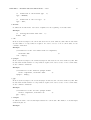
3.1
HELP — displaying a command manual
Display the on-line reference of SATELLITE commands.
usage : help( "com_name" )
com_name stands for a command name. It needs to be put in double quotation marks. For example, the
explanation of HELP command is displayed by the following:
[]SATELLITE[]~tom/rose:[63]% help("help") ←-
3.2
HEADER — displaying or modifying the header information of a data file
This command is for confirmation or alteration of a data file header information (such as data format,
index, etc.).
usage : header( file_name, mode )
file_name stands for a file name and mode is the integer that selects the mode (0: display, 1: modify).
The following example displays information about the data file test.dat on a display.
[]SATELLITE[]~tom/rose:[64]% header("test.dat", 0) ←-
3.3
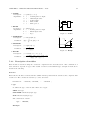
WAIT — interrupting the execution of a program
It pauses the batch processing until CR key is pressed.
usage : wait()
33
34
CHAPTER 3. SYSTEM MODULE — SYSTEM
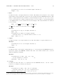
14
13
12
13th
11
12th
10
11th
9
10th
8
9th
7
8th
6
7th
5
6th
4
Time
5th
3
4th
2
3rd
1
2nd
1st
0th
13 14
11 12
9 10
7 8
5
6
3 4
1 2
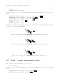
Figure 3.1: An example of using REFORM(1).
3.4
13 14
11 12
6th
9 10
5th
7 8
4th
5 6
3rd
3 4
Time
2nd
1 2
1st
0th
0
0 0 0
13 14 0 0
5 6 7 8
1
2
3
4
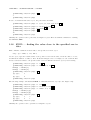
Figure 3.2: An example of using REFORM(2).
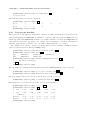
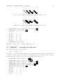
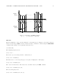
REFORM — changing the size or index of data
Command for the modification of an object format.
usage : y = reform( x, index )
x stands for an input object, y for output, and index for the index of y. As shown in Figure 3.1, for
example, we can change a 1-dimensional Series object a to a 2-dimensional Series object b by the following:
[]SATELLITE[]~tom/rose:[65]%
[]SATELLITE[]~tom/rose:[66]%
[ 0]:%
1
2
3
[ 5]:%
6
7
8
[10]:%
11
12
13
[]SATELLITE[]~tom/rose:[67]%
[]SATELLITE[]~tom/rose:[68]%
[0]:[0]%
1
2
[1]:[0]%
3
4
[2]:[0]%
5
6
[3]:[0]%
7
8
[4]:[0]%
9
10
[5]:[0]%
11
12
[6]:[0]%
13
14
[]SATELLITE[]~tom/rose:[69]%
a = 1~14 ←a ←4
5
9
10
14
b = reform(a,(7,2)) ←b ←-
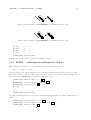
Conversion of 2-dimensional Series object b to 3-dimensional Series object c, shown in Figure 3.2, is
performed as follows. If the specified index size is bigger than the input object’s one, 0s are filled in the
tail of data.
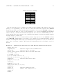
[]SATELLITE[]~tom/rose:[69]% c = reform(b,(3,2,4)) ←[]SATELLITE[]~tom/rose:[70]% c ←[0]:[0][0]%
1
2
3
4
[0]:[1][0]%
5
6
7
8
[1]:[0][0]%
9
10
11
12
[1]:[1][0]%
13
14
0
0
[2]:[0][0]%
0
0
0
0
[2]:[1][0]%
0
0
0
0
[]SATELLITE[]~tom/rose:[71]%
Similarly can be reformatted Snapshot objects.
35
CHAPTER 3. SYSTEM MODULE — SYSTEM
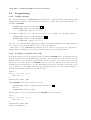
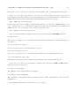
Figure 3.3: Buffer monitor.
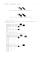
3.5
Figure 3.4: Window for setting up a range to
draw.
BM — data monitoring
This command displays a window for monitoring objects simultaneously while processing other commands.
usage : bm( x )
x stands for an object to monitor. Example:
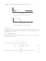
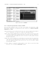
[]SATELLITE[]~tom/rose:[72]% bm(x) ←The example of the buffer monitor is in Figure 3.3. In this example, the object x has already been defined
by the following:
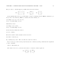
[]SATELLITE[]~tom/rose:[70]% t = 0~99 ←[]SATELLITE[]~tom/rose:[71]% x = sin(2*PI*t/100) ←Another window can be opened by clicking on the SCALE button. One can adjust scaling of a chart.
Figure 3.4 shows the window.
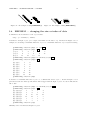
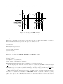
An example of 2-dimensional Series objects is given. First, we convert 1-dimensional Series object x
to 2-dimensional Series object y by REFORM as follows:
[]SATELLITE[]~tom/rose:[73]% y = reform(x,(2,50)) ←If we want to monitor y, we can proceed similarly as in the previous example,
[]SATELLITE[]~tom/rose:[74]% bm(y) ←The buffer monitor window of this example is shown in Figure 3.5. By clicking on the button >, the
chart is changed, as shown in Figure 3.6. Figure 3.5 is the chart of y:[0] and Figure 3.6 of y:[1]. That
is, Figure 3.5 corresponds to the chart from x:[0] to x:[49] and Figure 3.6 from x:[50] to x:[99].
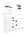
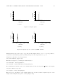
3.6
SAM — sampling frequency setting
This command defines a sampling frequency.
usage : sam( frequency )
36
CHAPTER 3. SYSTEM MODULE — SYSTEM
Figure 3.5: Window for monitoring y:[0].
Figure 3.6: Window for monitoring y:[1].
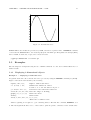
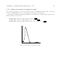
frequency is a sampling frequency. For example, define a Series object a as follows:
[]SATELLITE[]~tom/rose:[77]% a = 1~10 ←The chart of a, by using WOPEN, GRAPH, and AXIS commands, is shown in Figure 3.7. In this
case, the default sampling frequency is 1000Hz. Figure 3.8 displays the chart of a after changing the
sampling frequency as follows:
[]SATELLITE[]~tom/rose:[78]% sam(100) ←The sampling frequency set by SAM is referred in commands of ISPP module or GRAPH command
of GPM module.
3.7
CUT — selecting a subset of data
This command allows selection of specified subset of data contained in an object.
usage : y = cut( x, start, end )
x is the original object, y is the object picked out, start is the starting point, and end is the end point.
The following example selects a part of a 1-dimensional Series object a, as shown in Figure 3.9:
[]SATELLITE[]~tom/rose:[79]%
[]SATELLITE[]~tom/rose:[80]%
[0]:%
1
2
3
[5]:%
6
7
[]SATELLITE[]~tom/rose:[81]%
[]SATELLITE[]~tom/rose:[82]%
[0]:%
4
5
6
[]SATELLITE[]~tom/rose:[83]%
a = 1~7 ←a ←4
5
b = cut(a,3,5) ←b ←-
One cannot obtain the proper result if the start point is replaced with the end one as follows:
[]SATELLITE[]~tom/rose:[81]% b = cut(a,5,3) ←One can also select a part of the 2-dimensional Series object b by the following (see also Figure 3.10):
37
2.0
4.0
6.0
8.0
10.0
12.0
CHAPTER 3. SYSTEM MODULE — SYSTEM
0.0
2.0
4.0
6.0
8.0
10.0
2.0
4.0
6.0
8.0
10.0
12.0
Figure 3.7: A graphic using the sampling frequency = 1000Hz (default).
0.0
200.0
400.0
600.0
800.0
1000.0
Figure 3.8: A graphic using the sampling frequency = 10Hz.
38
CHAPTER 3. SYSTEM MODULE — SYSTEM
7
6
6th
5
5th
4
4th
3
3rd
2
Time
2nd
1
1st
0th
6
5
4
Figure 3.9: An example of using CUT on 1-dimensional Series object.
13 14
11 12
6th
9 10
5th
7 8
4th
5 6
3rd
3 4
Time
2nd
1 2
1st
0th
11
9
7
Figure 3.10: An example of using CUT on 2-dimensional Series object.
[]SATELLITE[]~tom/rose:[85]%
[]SATELLITE[]~tom/rose:[86]%
[]SATELLITE[]~tom/rose:[87]%
[]SATELLITE[]~tom/rose:[88]%
[0]:[0]%
7
[1]:[0]%
9
[2]:[0]%
11
[]SATELLITE[]~tom/rose:[89]%
a
b
c
c
= 1~14 ←= reform(a,(7,2)) ←= cut(b,(3,0),(5,0)) ←←-
Similarly, selection can be performed on Snapshot objects.
3.8
PUT — replacing old data with new one
This command replaces a part of an object with another one.
usage : z = put( x, y, index )
x is the original object, y is the object to insert into x, z is the object after replacement, and index is
the position where to put y. The size of the object z is the same as that of x. For example, as shown in
Figure 3.11, replacement of a part of a 1-dimensional Series object a by b can be performed as follows:
[]SATELLITE[]~tom/rose:[89]%
[]SATELLITE[]~tom/rose:[90]%
[]SATELLITE[]~tom/rose:[91]%
[]SATELLITE[]~tom/rose:[92]%
[0]:%
1
2
3
[5]:%
13
14
[]SATELLITE[]~tom/rose:[93]%
a
b
c
c
= 1~7 ←= 11~17 ←= put(a,b,3) ←←11
12
The next example is the case of 2-dimensional Series object replacement, as shown in Figure 3.12.
[]SATELLITE[]~tom/rose:[23]%
[]SATELLITE[]~tom/rose:[24]%
[]SATELLITE[]~tom/rose:[25]%
[]SATELLITE[]~tom/rose:[26]%
a = 1~14 ←b = 31~36 ←ar = reform(a,(7,2)) ←br = reform(b,(3,2)) ←-
39
CHAPTER 3. SYSTEM MODULE — SYSTEM
7
6
6th
5
5th
4
4th
3
3rd
2
Time
2nd
1
1st
0th
17
14
16
13
15
14
12
11
13
12
3
2
11
1
Figure 3.11: An example of using PUT on 1-dimensional Series object.
13 14
11 12
6th
9 10
5th
7 8
4th
5 6
3rd
3 4
Time
2nd
1 2
1st
0th
35 36
33 34
31 32
13 14
11 12
35 36
33 34
31 32
3 4
1 2
Figure 3.12: An example of using PUT on 2-dimensional Series object.
[]SATELLITE[]~tom/rose:[27]% c = put(ar,br,(2,0)) ←[]SATELLITE[]~tom/rose:[28]% c ←[0]:[0]%
1
2
[1]:[0]%
3
4
[2]:[0]%
30
31
[3]:[0]%
32
33
[4]:[0]%
34
35
[5]:[0]%
11
12
[6]:[0]%
13
14
[]SATELLITE[]~tom/rose:[29]%
Similarly, the operation can be performed on Snapshot objects.
3.9
MERGE — merging two data sets
This command merges two objects together.
usage : z = merge( x, y )
x and y are the objects to link, and z is the final object in which y is attached at the end x. The subindex
of x must be equal to the y’s one in the case of multi-dimensional objects. The example of merging
2-dimensional Series objects ar and br is shown below and depicted Figure 3.13:
[]SATELLITE[]~tom/rose:[29]%
[]SATELLITE[]~tom/rose:[30]%
[]SATELLITE[]~tom/rose:[31]%
[]SATELLITE[]~tom/rose:[32]%
[]SATELLITE[]~tom/rose:[33]%
[]SATELLITE[]~tom/rose:[34]%
[0]:[0]%
1
2
[1]:[0]%
3
4
[2]:[0]%
5
6
[3]:[0]%
7
8
[4]:[0]%
30
31
a = 1~8 ←b = 31~36 ←ar = reform(a,(4,2)) ←br = reform(b,(3,2)) ←c = merge(ar,br) ←c ←-
40
CHAPTER 3. SYSTEM MODULE — SYSTEM
7 8
5 6
3rd
3 4
Time
2nd
1 2
1st
0th
35
36
33
34
31 32
35 36
33 34
31 32
7 8
5 6
3 4
1 2
Figure 3.13: An example of using MERGE on 2-dimensional Series object.
[5]:[0]%
32
33
[6]:[0]%
34
35
[]SATELLITE[]~tom/rose:[35]%
Similarly Snapshot objects.
3.10
FILL — filling data with a specified value
This command fills a part of an object with a particular value.
usage : y = fill( x, start, end, value )
x is the original object, y is the final object, and start and end are the start and end points for filling
the value. All range in x specified by start and end is filled with the same value value. If we want to
fill a part of 1-dimensional Series object a with 20 as shown in Figure 3.14, we proceed as follows:
[]SATELLITE[]~tom/rose:[35]% a = 1~7 ←[]SATELLITE[]~tom/rose:[36]% b = fill(a,3,5,20) ←[]SATELLITE[]~tom/rose:[37]% b ←[0]:%
1
2
3
20
20
[5]:%
20
7
[]SATELLITE[]~tom/rose:[38]%
The example of filling 2-dimensional Series object follows (see also Figure 3.15):
[]SATELLITE[]~tom/rose:[38]%
[]SATELLITE[]~tom/rose:[39]%
[]SATELLITE[]~tom/rose:[40]%
[]SATELLITE[]~tom/rose:[41]%
[0]:[0]%
1
2
[1]:[0]%
3
4
[2]:[0]%
5
6
[3]:[0]%
30
8
[4]:[0]%
30
10
[5]:[0]%
30
12
[6]:[0]%
13
14
[]SATELLITE[]~tom/rose:[42]%
a
b
c
c
= 1~14 ←= reform(a,(7,2)) ←= fill(b,(3,0),(5,0),30) ←←-
Similarly, the operation can be performed on Snapshot objects.
3.11
ZERO — filling data with 0
This command fills a part of an object with 0.
41
CHAPTER 3. SYSTEM MODULE — SYSTEM
7
6
6th
5
5th
4
4th
3
3rd
2
Time
2nd
1
1st
0th
7
20
20
20
3
2
1
Figure 3.14: An example of using FILL on 1-dimensional Series object.
13 14
11 12
6th
9 10
5th
7 8
4th
5 6
3rd
3 4
Time
2nd
1 2
1st
0th
13 14
11 12
30 10
30 8
30 6
3 4
1 2
Figure 3.15: An example of using FILL on 2-dimensional Series object.
usage : y = zero( x, start, end )
x is the original object, y is the filled object, and start and end are the start and end points. The range
in x specified by start and end is filled with 0. The following example is similar to the FILL’s one as
shown in Figure 3.16, except the specified value 20 is replaced with 0:
[]SATELLITE[]~tom/rose:[42]% a = 1~7 ←[]SATELLITE[]~tom/rose:[43]% b = zero(a,3,5) ←[]SATELLITE[]~tom/rose:[44]% b ←[0]:%
1
2
3
0
0
[5]:%
0
7
[]SATELLITE[]~tom/rose:[45]%
In the case of 2-dimensional Series object, as shown in Figure 3.17, the following example is quite similar
to previous one.
[]SATELLITE[]~tom/rose:[45]%
[]SATELLITE[]~tom/rose:[46]%
[]SATELLITE[]~tom/rose:[47]%
[]SATELLITE[]~tom/rose:[48]%
[0]:[0]%
1
2
[1]:[0]%
3
4
[2]:[0]%
5
6
[3]:[0]%
0
8
[4]:[0]%
0
10
[5]:[0]%
0
12
[6]:[0]%
13
14
[]SATELLITE[]~tom/rose:[49]%
a
b
c
c
= 1~14 ←= reform(a,(7,2)) ←= zero(b,(3,0),(5,0)) ←←-
Similarly, the operation can be performed on Snapshot objects.
3.12
REVERSE — reversing the order of data
This command reverses the order of data in an object.
42
CHAPTER 3. SYSTEM MODULE — SYSTEM
7
6
6th
5
5th
4
4th
3
3rd
2
Time
2nd
1
1st
0th
7
0
0
0
3
2
1
Figure 3.16: An example of using ZERO on 1-dimensional Series object.
13 14
11 12
6th
9 10
5th
7 8
4th
5 6
3rd
3 4
Time
2nd
1 2
1st
0th
13 14
11 12
0 10
0 8
0 6
3 4
1 2
Figure 3.17: An example of using ZERO on 2-dimensional Series object.
usage : y = reverse( x )
x is the original object, and y is the reversed one. For example, the reversed 1-dimensional Series object
a is obtained by the following:
[]SATELLITE[]~tom/rose:[49]%
[]SATELLITE[]~tom/rose:[50]%
[]SATELLITE[]~tom/rose:[51]%
[0]:%
1
2
3
[5]:%
6
7
[]SATELLITE[]~tom/rose:[52]%
[0]:%
7
6
5
[5]:%
2
1
[]SATELLITE[]~tom/rose:[53]%
a = 1~7 ←b = reverse(a) ←a ←4
5
b ←4
3
The case of 2-dimensional Series object (see also Figure 3.18):
[]SATELLITE[]~tom/rose:[54]%
[]SATELLITE[]~tom/rose:[55]%
[]SATELLITE[]~tom/rose:[56]%
[0]:[0]%
1
2
[1]:[0]%
3
4
[2]:[0]%
5
6
[3]:[0]%
7
8
[4]:[0]%
9
10
[5]:[0]%
11
12
[6]:[0]%
13
14
[]SATELLITE[]~tom/rose:[57]%
[]SATELLITE[]~tom/rose:[58]%
[0]:[0]%
14
13
[1]:[0]%
12
11
[2]:[0]%
10
9
[3]:[0]%
8
7
[4]:[0]%
6
5
a = 1~14 ←b = reform(a,(7,2)) ←b ←-
c = reverse(b) ←c ←-
43
CHAPTER 3. SYSTEM MODULE — SYSTEM
13 14
11 12
6th
9 10
5th
7 8
4th
5 6
3rd
3 4
Time
2nd
1 2
1st
0th
2
1
4
3
6 5
8 7
10 9
12 11
14 13
Figure 3.18: An example of using REVERSE on 2-dimensional Series object.
[5]:[0]%
4
3
[6]:[0]%
2
1
[]SATELLITE[]~tom/rose:[59]%
Similarly, the operation can be performed on Snapshot objects.
3.13
ROTATE — rotating data
This command moves the head pointer of an object to the specified position.
usage : y = rotate( x, index )
x is the original object, y is the rotated object, and index is the position of the front. An example is
shown in Figure 3.19:
[]SATELLITE[]~tom/rose:[59]%
[]SATELLITE[]~tom/rose:[60]%
[0]:%
1
2
3
[5]:%
6
7
[]SATELLITE[]~tom/rose:[61]%
[]SATELLITE[]~tom/rose:[62]%
[0]:%
4
5
6
[5]:%
2
3
[]SATELLITE[]~tom/rose:[63]%
a = 1~7 ←a ←4
5
b = rotate(a,3) ←b ←7
1
The following example is for 2-dimensional Series object, as shown in Figure 3.20.
[]SATELLITE[]~tom/rose:[63]%
[]SATELLITE[]~tom/rose:[64]%
[]SATELLITE[]~tom/rose:[65]%
[0]:[0]%
1
2
[1]:[0]%
3
4
[2]:[0]%
5
6
[3]:[0]%
7
8
[4]:[0]%
9
10
[5]:[0]%
11
12
[6]:[0]%
13
14
[]SATELLITE[]~tom/rose:[66]%
[]SATELLITE[]~tom/rose:[67]%
[0]:[0]%
7
8
[1]:[0]%
9
10
[2]:[0]%
11
12
a = 1~14 ←b = reform(a,(7,2)) ←b ←-
c = rotate(b,(3,0)) ←c ←-
44
CHAPTER 3. SYSTEM MODULE — SYSTEM
7
6
6th
5
5th
4
4th
3
3rd
2
Time
2nd
1
1st
0th
3
2
1
7
6
5
4
Figure 3.19: An example of using ROTATE on 1-dimensional Series object.
13 14
11 12
6th
9 10
5th
7 8
4th
5 6
3 4
3rd
1 2
Time
2nd
1st
0th
5
6
3
4
1
2
13 14
11 12
9 10
7 8
Figure 3.20: An example of using ROTATE on 2-dimensional Series object.
[3]:[0]%
13
14
[4]:[0]%
1
2
[5]:[0]%
3
4
[6]:[0]%
5
6
[]SATELLITE[]~tom/rose:[68]%
Similarly, the operation can be performed on Snapshot objects.
3.14
MABI — selecting the subsequence of data
This command selects from an object a subsequence of data specified by interval.
usage : y = mabi( x, step )
x is the original object, y is the resulting object, and step is the interval (at interval of step − 1 points).
There is no difference between x and y in the case where step = 0 or 1. The following example, and
Figure 3.21, shows MABI function on 1-dimensional Series object:
[]SATELLITE[]~tom/rose:[68]% a = 1~7 ←[]SATELLITE[]~tom/rose:[69]% b = mabi(a,2) ←[]SATELLITE[]~tom/rose:[70]% b ←[7]->[4]
[0]:%
1
3
5
[]SATELLITE[]~tom/rose:[71]%
7
Selecting 2-dimensional Series object at some intervals is shown in Figure 3.22. The commands are as
follows:
[]SATELLITE[]~tom/rose:[71]% a = 1~21 ←[]SATELLITE[]~tom/rose:[72]% b = reform(a,(7,3)) ←[]SATELLITE[]~tom/rose:[73]% b ←-
45
CHAPTER 3. SYSTEM MODULE — SYSTEM
7
6
6th
5
5th
4
4th
3
3rd
2
1
Time
2nd
1st
0th
7
5
3
1
Figure 3.21: An example of using MABI on 1-dimensional Series object.
19 20 21
6th
16 17 18
13 14 15
5th
10 11 12
4th
7 8 9
3rd
4 5 6
Time
2nd
1 2 3
1st
0th
19 21
10 12
1 3
Figure 3.22: An example of using MABI on 2-dimensional Series object.
[0]:[0]%
1
2
3
[1]:[0]%
4
5
6
[2]:[0]%
7
8
9
[3]:[0]%
10
11
12
[4]:[0]%
13
14
15
[5]:[0]%
16
17
18
[6]:[0]%
19
20
21
[]SATELLITE[]~tom/rose:[74]% c = mabi(b,(3,2)) ←[]SATELLITE[]~tom/rose:[75]% c ←[7][3]->[3][2]
[0]:[0]%
1
3
[1]:[0]%
10
12
[2]:[0]%
19
21
[]SATELLITE[]~tom/rose:[76]%
Similarly, the operation can be performed on Snapshot objects.
3.15
GET — getting a value at the specified position of data
This function reads a value at the particular position of an object.
usage : y = get( x, position )
x is an object, and y is the value at position. A simple example is shown as follows (see also Figure
3.23):
[]SATELLITE[]~tom/rose:[77]% a = 1~7 ←[]SATELLITE[]~tom/rose:[78]% b = get(a,3) ←[]SATELLITE[]~tom/rose:[79]% b ←-
46
CHAPTER 3. SYSTEM MODULE — SYSTEM
7
6
6th
5
5th
4
4th
3
3rd
2
Time
2nd
1
1st
0th
4
Figure 3.23: An example of using GET on 1-dimensional Series object.
13 14
11 12
6th
9 10
5th
7 8
4th
5 6
3rd
3 4
Time
2nd
1 2
1st
0th
7
Figure 3.24: An example of using GET on 2-dimensional Series object.
4
[]SATELLITE[]~tom/rose:[80]%
In case of 2-dimensional Series object (as shown in Figure 3.24), we have
[]SATELLITE[]~tom/rose:[80]%
[]SATELLITE[]~tom/rose:[81]%
[]SATELLITE[]~tom/rose:[82]%
[]SATELLITE[]~tom/rose:[83]%
7
[]SATELLITE[]~tom/rose:[84]%
a
b
c
c
= 1~14 ←= reform(a,(7,2)) ←= get(b,(3,0)) ←←-
Similarly, the operation can be performed on Snapshot objects.
3.16
MAXPOS — getting the position of the maximum in
data
This command obtains the position of the maximum in a object.
usage : y = maxpos( x, num )
x is an object, y is the Series object, and num is the number of positions to consider. For example, as
shown in Figure 3.25, if we need to obtain the position of the maximum in the 1-dimensional Series object
a, then,
[]SATELLITE[]~tom/rose:[84]% a =(3,7,5,1,6,2,4) ←[]SATELLITE[]~tom/rose:[85]% c = maxpos(a,1) ←[]SATELLITE[]~tom/rose:[86]% c ←1
[]SATELLITE[]~tom/rose:[87]%
To get the positions of the 1st and 2nd maxima in a, as shown in Figure 3.26, is done by the following:
[]SATELLITE[]~tom/rose:[87]% c = maxpos(a,2) ←[]SATELLITE[]~tom/rose:[88]% c ←[0]:[0]%
1
47
CHAPTER 3. SYSTEM MODULE — SYSTEM
[1]:[0]%
4
[]SATELLITE[]~tom/rose:[89]%
As shown in Figure 3.27, to get the position of the maximum in 2-dimensional Series object b proceed as
follows:
[]SATELLITE[]~tom/rose:[18]%
[]SATELLITE[]~tom/rose:[19]%
[]SATELLITE[]~tom/rose:[20]%
[]SATELLITE[]~tom/rose:[21]%
[0]:[0]%
4
0
[]SATELLITE[]~tom/rose:[22]%
a
b
c
c
= (7,13,1,3,12,6,11,4,14,2) ←= reform(a,(5,2)) ←= maxpos(b,1) ←←-
Similarly, the operation can be performed on Snapshot objects. There is a similar command for obtaining
the position of the minimum; MINPOS.
4
2
6th
6
5th
1
4th
5
3rd
7
Time
2nd
3
1st
0th
7
Figure 3.25: An example of using MAXPOS on 1-dimensional Series object(1).
4
2
6th
6
5th
1
4th
5
3rd
7
Time
2nd
3
1st
0th
6
Max
7
Figure 3.26: An example of using MAXPOS on 1-dimensional Series object(2).
5 8
9 10
6th
14 2
5th
11 4
4th
12 6
3rd
1 3
Time
2nd
7 13
1st
0th
14
Figure 3.27: An example of using MAXPOS on 2-dimensional Series object.
3.17
MAX — getting the maximum of data
This command obtains the maximum value of an object.
usage : y = max( x )
x is the object, and y is the maximum value of it. In case of 1-dimensional Series object, the example
follows:
[]SATELLITE[]~tom/rose:[23]% a =(3,7,5,1,6,2,4) ←[]SATELLITE[]~tom/rose:[24]% c = max(a) ←-
CHAPTER 3. SYSTEM MODULE — SYSTEM
48
[]SATELLITE[]~tom/rose:[25]% c ←7
[]SATELLITE[]~tom/rose:[26]%
In case of a 2-dimensional Series object, the performance is similar.
[]SATELLITE[]~tom/rose:[26]%
[]SATELLITE[]~tom/rose:[27]%
[]SATELLITE[]~tom/rose:[28]%
[]SATELLITE[]~tom/rose:[29]%
14
[]SATELLITE[]~tom/rose:[30]%
a
b
c
c
= (7,13,1,3,12,6,11,4,14,2) ←= reform(a,(5,2)) ←= max(b) ←←-
Similarly, the operation can be performed on Snapshot objects. There is a similar command for obtaining
the minimum; MIN.
3.18
FIND — finding the value close to the specified one in
data
This command obtains the nearest value to the specified one in an object.
usage : ip = find( x, val, num )
x is an object, ip is the returned value of the position of the nearest value, val is the value to locate,
and num is the number of values to find. As shown in Figure 3.28, for example, we can obtain the first
and second nearest values to the specified value 5.8 in a 1-dimensional Series object by the following:
[]SATELLITE[]~tom/rose:[30]% a = 1~7 ←[]SATELLITE[]~tom/rose:[31]% c = find(a, 5.8, 2) ←DATA[6] -- POINT:[5]
DATA[5] -- POINT:[4]
[]SATELLITE[]~tom/rose:[32]% c ←[0]:[0]%
5
[1]:[0]%
4
[]SATELLITE[]~tom/rose:[33]%
The following example demonstrates FIND on 2-dimensional Series object (see also Figure 3.29):
[]SATELLITE[]~tom/rose:[33]%
[]SATELLITE[]~tom/rose:[34]%
[]SATELLITE[]~tom/rose:[35]%
DATA[7] -- POINT:[3][0]
DATA[6] -- POINT:[2][1]
[]SATELLITE[]~tom/rose:[36]%
[0]:[0]%
3
0
[1]:[0]%
2
1
[]SATELLITE[]~tom/rose:[37]%
a = 1~14 ←b = reform(a,(7,2)) ←c = find(b, 6.8, 2) ←-
c ←-
Similarly, the operation can be performed on Snapshot objects.
49
CHAPTER 3. SYSTEM MODULE — SYSTEM
7
6th
6
5
5th
4
4th
3
3rd
2
Time
2nd
1
1st
0th
5
4
Figure 3.28: An example of using FIND on 1-dimensional Series object.
13 14
11 12
6th
9 10
5th
7 8
4th
5 6
3rd
3 4
Time
2nd
1 2
1st
0th
7
6
Figure 3.29: An example of using FIND on 2-dimensional Series object.
Chapter 4
Interactive Signal Processing
Package — ISPP
ISPP is the core module of SATELLITE. A lot of processing functions are represented by commands, which
cover the methodology of the digital signal processing such as the preprocessing by window functions,
FFT, spectrum analysis by linear prediction model, filtering, cepstrum analysis, etc. All commands
require to store data or data files. One can analyze data multilaterally using the signal processing or
statistical techniques.
4.1
The command system of ISPP
The commands of ISPP are classified into the categories shown in Table 4.1 and 4.2. By combining the
commands with fundamental functions, it is possible to carry out complicated analysis.
4.2
Examples to use
The fundamental use of ISPP is described, by referring to Fourier transform, filtering, and matrix operation.
4.2.1
Fourier transform
Fourier transform of a signal is shown. Signal is synthesized two sinusoidal waves overlapped by noise.
Generation of data
(1) Generation of a sinusoidal wave:
(1) t = 0~1999/2000;
Data is stored in the Series object t.
(2) a = 5*sin(2*PI*20*t) + 3;
b = 3*sin(2*PI*50*t) + 3;
The sine waves with DC in which their frequencies and amplitude values are different from each other
are stored in the Series objects a and b.
50
CHAPTER 4. INTERACTIVE SIGNAL PROCESSING PACKAGE — ISPP
Table 4.1: ISPP commands (1).
argen
gauss2
arand
mnrand
nrand
urand
dccut
norm
shift
interp
akima
spline
average
integ
det
eigen
inv
mul
trans
nmeq
Data generation
Data generation by AR model
Generation of 2-dimensional Gaussian distribution function
Generation of random data with optional probability distribution
Generation of multi-dimensional Gaussian random data
Generation of Gaussian random data
Generation of uniform random data
Data operation
DC removal from data
Data normalization
Shifting the whole data so that the specified value is consistent
with a specified element of the data
Data interpolation
Interpolation of 2-dimensional data
Interpolation of 1-dimensional data by the Akima’s method
Interpolation of 1-dimensional data by the natural cubic spline
Arithmetic operation
Calculation of the arithmetic mean of data
Calculation of the sum of data
Calculation of the determinant
Calculation of eigenvalues and eigenvectors
Calculation of the inverse matrix
Calculation of the product of two matrices
Calculation of the transposed matrix
Solving the normal equation
Table 4.2: ISPP commands (2).
bpbtw
burg
cep
fftc
fftn
fir
firmake
hil
hpbtw
icep
iir
iircoef
levin
lpbtw
phase
pole
power
rank
spcf
window
Data analysis
Design of IIR-type band-pass filter with the Butterworth property
Calculation of power spectra by the Burg method
Calculation of complex cepstrum
Complex Fourier transform
Complex Fourier transform for multi-dimensional data
Filtering by FIR-type filter
Design of FIR-type filter
Hilbert transform
Design of IIR-type high-pass filter with the Butterworth property
Inverse cepstrum analysis
Filtering by IIR-type filter
Calculation of the coefficients of IIR-type filter from zero points and poles
Calculation of power spectra by the Levinson-Durbin’s algorithm
Design of IIR-type low-pass filter with Butterworth property
Calculation of the phase of a complex number
Calculation of poles from AR coefficients
Calculation of the gain of a complex number
Calculation of histogram and the Gaussian density function value from data
Calculation of power spectrum and phase of data
Window processing for data
51
CHAPTER 4. INTERACTIVE SIGNAL PROCESSING PACKAGE — ISPP
(2) Selecting a part of data
wave.
52
of 1024-point from the 0th point to the 1023rd point of a sinusoidal
(3.1) acut =
bcut =
Series objects which store picked data are set.
(3.2) acut = cut(a,
bcut = cut(b,
Original objects are set.
(3.3) acut = cut(a,0
bcut = cut(b,0
Each starting point is set.
(3.4) acut = cut(a,0,1023);
bcut = cut(b,0,1023);
Each ending point is set.
By the above procedure, the selected data are stored in the Series objects acut and bcut.
(3) Generation of random numbers: We use NRAND command to generate the normal random
numbers.
(4.1) nois =
The Series object that stores generated random numbers is set.
(4.2) nois = nrand(1024,
The number of datum point to generate is set.
(4.3) nois = nrand(1024,1
The initial value to generate random numbers is set (This must be an odd number).
(4.4) nois = nrand(1024,1,0
The mean value of random numbers is set.
(4.5) nois = nrand(1024,1,0,1);
The variance of the random number is set.
By the above procedure, 1024-point standard normal random number data are stored in the Series
object nois. Furthermore, the URAND command is used for generating the uniform random numbers.
53
-20
0
20
CHAPTER 4. INTERACTIVE SIGNAL PROCESSING PACKAGE — ISPP
0
200
400
600
800
1000
Time[msec]
Figure 4.1: Waveform of the synthetic signal.
(4) Synthesis of signals: The signals obtained by the above procedures are synthesized as follows:
(5.1) data =
The Series object that stores the synthetic signal is set.
(5.2) data = acut + bcut + nois;
Signals are synthesized.
Mixture of two sine waves and normal random numbers is stored in the Series object data. The
waveform of the synthetic signal is shown in Figure 4.1.
Preprocessing of data
The methods of DC removal and window processing are shown below.
(1) Removal of DC: The DCCUT command is used for removing the DC of data.
(1.1) data1 =
The Series object that stores the data after removing DC is set.
(1.2) data1 = dccut(data);
The original object is set.
By the above procedure, the data with removed DC is stored in the Series object data1. The signal
waveform is shown in Figure 4.2.
(2) Window processing: We use the WINDOW command for the window processing.
(2.1) data2 =
The Series object that stores the data after the window processing.
(2.2) data2 = window(data1,
54
-20
0
20
CHAPTER 4. INTERACTIVE SIGNAL PROCESSING PACKAGE — ISPP
0
200
400
600
800
1000
Time[msec]
-20
0
20
Figure 4.2: Signal waveform after the removal of DC.
0
200
400
600
800
1000
Time[msec]
Figure 4.3: Signal waveform after the window processing.
The original object is set.
(2.3) data2 = window(data1,1,
The type of the window (1: Humming window, 2: Hanning window, 3: Blackman window, 4: Triangle
window) is set.
(2.4) data2 = window(data1,1,0);
1 is set if we want to correct data so that both integrated values of data before and after the window
processing become equal, but 0 if not.
By the above procedure, the data after the window processing is performed is stored in the Series
object data2. The signal waveform is shown in Figure 4.3.
Fourier transform
(1) Fourier transform: Using the FFTC command, it is possible to carry out Fourier transform and
inverse Fourier transform for complex number data. Since the FFT algorithm is used for the Fourier
transform, the number of data must be the power of 2.
55
-1000
0
1000
CHAPTER 4. INTERACTIVE SIGNAL PROCESSING PACKAGE — ISPP
0
20
40
60
80
100
Frequency[Hz]
Figure 4.4: The signal waveform after Fourier transform (black line: the real parts of data, gray line: the
imaginary parts of data).
(1) series Rout,Iout;
The Series object that stores the real part and the imaginary part of an output time series is defined.
(2) rei = 0~1023*0;
In the case where the imaginary part of the original signal does not exist, 1024 zeros are stored in the
Series object rei.
(3.1) fftc(P,
The flag for calculation (P: Fourier transform, I: Inverse Fourier transform) is set.
(3.2) fftc(P,data2,
The real part of the original object is set.
(3.3) fftc(P,data2,rei,
The imaginary part of the original object is set.
(3.4) fftc(P,data2,rei,Rout,
The Series object that stores the real part of the data after Fourier transform is set.
(3.5) fftc(P,data2,rei,Rout,Iout);
The Series object that stores the imaginary part of the data after Fourier transform is set.
By the above procedure, the processed data is stored in the Series objects Rout, Iout. The signal
waveform after Fourier transform is shown in Figure 4.4.
20
56
0
10
* 10
5
CHAPTER 4. INTERACTIVE SIGNAL PROCESSING PACKAGE — ISPP
0
20
40
60
80
100
Frequency[Hz]
Figure 4.5: Power spectrum.
(2) Power spectra: The POWER command is used for adding two squared objects. Using this
command, we can obtain the power spectrum of the original time series from the real part and the
imaginary part of the data after the Fourier transform.
(4.1) pw =
The Series object that stores the obtained power spectrum is set.
(4.2) pw = power(Rout,
The real part of the data after Fourier transform is set.
(4.3) pw = power(Rout,Iout);
The imaginary part of the data after Fourier transform is set.
The power spectrum data is stored in the Series object pw, and shown in Figure 4.5.
(3) Phase property: The PHASE command is used for obtaining the phase of the original time
series from the real part and the imaginary part of the data after the Fourier transform.
(5.1) phs =
The Series object that stores the obtained phase is set.
(5.2) phs = phase(Rout,
The real part of the data after Fourier transform is set.
(5.3) phs = phase(Rout,Iout,
The imaginary part of the data after Fourier transform is set.
(5.4) phs = phase(Rout,Iout,D,
The type of the output phase (D: degree, O: radian) is set.
(5.5) phs = phase(Rout,Iout,D,U);
U is set if we want to perform the phase rehydration, but O if not.
By the above procedure, the phase data is stored in the Series object phs.
CHAPTER 4. INTERACTIVE SIGNAL PROCESSING PACKAGE — ISPP
57
Method for obtaining the power spectrum and the phase of the original data
Using the SPCF command, we can obtain both the power spectrum and the phase from an input time
series. The procedure is shown below.
(1) series pw,phs;
The Series objects that store the power spectrum and the phase are defined.
(2.1) spcf(data2,
The original time series is set.
(2.2) spcf(data2,pw,
The Series object that stores the obtained power spectrum is set.
(2.3) spcf(data2,pw,phs);
The Series object that stores the obtained phase is set.
The power spectrum and the phase data are stored in the Series objects pw and phs by the above.
4.2.2
Filtering
MA filter
Using the moving average method, the procedure for smoothing the source signal is shown as follows.
(1) coef = (1/5, 1/5, 1/5, 1/5, 1/5);
The coefficient vector of the filter is set.
(2.1) output =
The object that stores the smoothed signal is set.
(2.2) output = fir(coef,
The source signal is smoothed by using the FIR command. First, the coefficient of the filter coef is set.
(2.3) output = fir(coef, input);
The original signal input is set.
By the above procedure, the smoothed data is stored in the Series object output. The FIR command
carries out the processing shown in Figure 4.6. Therefore, the number of the filter coefficients (the order
of the filter) must be the odd number (it is assumed that this value is equal to 2n + 1). Besides, the
original data form the (n + 1)-th point is used for filtering, because the data from the beginning to the
n-th point is not possible to deal with precisely. Similarly the final data, the ones to the (n + 1)-th point
from behind is ignored.
58
CHAPTER 4. INTERACTIVE SIGNAL PROCESSING PACKAGE — ISPP
Input
Series
a1
a2
a3
a4
Σ
a5
a1
Move
a2
a3
a4
a5
Time
Σ
Output
Series
Copy
Copy
Time
0
Start
End
Figure 4.6: Filtering by the FIR command.
(a1 , a2 , · · · , a5 are the filter coefficients)
FIR filter
When the FIR filter of the low-pass, high-pass or band-pass type is designed by the window function
method, the filtering by FIR is carried out after the filter coefficient is obtained using the FIRMAKE
command. The example of a low-pass filter is shown below.
(1) sam(1024);
The sampling frequency is set.
(2.1) coef =
The Series object for storing the filter coefficients is set.
(2.2) coef = firmake(1,
The filter is set to be the low-pass type (1: Low-pass, 2: High-pass, 3: Band-pass).
(2.3) coef = firmake(1,11,
The order of the filter is set. The value is the odd number used by the FIR command.
(2.4) coef = firmake(1,11,100,
The cut-off frequency is set.
(2.5) coef = firmake(1,11,100,3);
CHAPTER 4. INTERACTIVE SIGNAL PROCESSING PACKAGE — ISPP
59
The type of the window function is set (0: Rectangle window, 1: Hanning window, 2: Humming window,
3: Blackman window, 4: Kayser window).
By the above procedure, the coefficients of the 11th-order FIR-type low-pass filter with the cut-off
frequency 100Hz is stored in the Series object coef. Similarly can be obtained high-pass type filter:
coef = firmake(2,11,400,3);
In this example, the 11th-order FIR-type high-pass filter with the cut-off frequency 400Hz is designed.
Band-pass filter with the cut-off frequencies 100Hz and 400Hz, and the order 11, for example, is obtained
as follows:
coef = firmake(3,11,(100,400),3);
Then, filtering can be performed by the FIR command with the coefficients coef as shown below.
(3) output = fir(coef,input);
IIR filter
In order to design an IIR filter of the low-pass, high-pass or band-pass type with the Butterworth
characteristics, it is first necessary to obtain zero points, poles, and gain of the transfer function using
the LPBTW, HPBTW, or BPBTW command, respectively. Then, filtering is carried out by using
FIR and IIR, after the zero points and poles are converted into the filter coefficients by the IIRCOEF
command. The example of a low-pass filter is shown below.
(1) sam(1024);
The sampling frequency is set.
(2) series zr,zi,pr,pi;
The Series objects for storing the zero points and poles of the transfer function are defined.
(3.1) gain =
The Scalar object for storing the gain of the designed filter is set.
(3.2) gain = lpbtw(100,
The cut-off frequency is set.
(3.3) gain = lpbtw(100,13,
The order of the filter is set. This value must be odd number (the maximum is 101).
(3.4) gain = lpbtw(100,13,zr,zi,
The Series objects for storing the zero points (real part and imaginary part) of the transfer function are
set.
(3.5) gain = lpbtw(100,13,zr,zi,pr,pi);
CHAPTER 4. INTERACTIVE SIGNAL PROCESSING PACKAGE — ISPP
60
The Series objects for storing the poles (real part and imaginary part) of the transfer function are set.
By the above procedure, it is possible to obtain the zero points zr and zi, the poles pr and pi, and
the gain gain of the transfer function of the 13th-order IIR-type low-pass filter with the cut-off frequency
100Hz, with the Butterworth characteristics. The high-pass filter can be set as follows:
gain = hpbtw(400,13,zr,zi,pr,pi);
In this example, the 13th-order IIR-type high-pass filter with the cut-off frequency 400Hz is designed. In
case of band-pass type, two cut-off frequencies must be set. When the cut-off frequencies are 100Hz and
400Hz, and the order of the filter is 13, for example, the following is set:
gain = bpbtw(100,400,13,zr,zi,pr,pi);
Next, we calculate the filter coefficients from zr, zi, pr, and pi using the IIRCOEF command.
(4) series a,b;
The Series objects that store the coefficients of the denominator and numerator of the transfer function
are defined.
(5.1) iircoef(zr,zi,pi,pr,
The zero points and poles of the transfer function are set.
(5.2) iircoef(zr,zi,pr,pi,a,
The Series object that stores the coefficients of the denominator of the transfer function is set.
(5.3) iircoef(zr,zi,pr,pi,a,b);
The Series object that stores the coefficients of the numerator of the transfer function is set.
By the above procedure, the obtained filter coefficients can be used in both FIR and IIR. Finally,
filtering is carried out as follows.
(6) temp = fir(b,input);
The numerator of the transfer function is calculated.
(7) output = iir(a,temp)*gain;
The denominator of the transfer function is calculated, and the result of the filtering is obtained by gain
multiplication.
The signal after filtering is stored in the Series object output.
61
CHAPTER 4. INTERACTIVE SIGNAL PROCESSING PACKAGE — ISPP
Input
Series
Time
Σ
Move
a1
a2
a3
a4
Σ
a5
a2
a1
a3
a4
a5
Output
Series
Time
0
Start
End
Figure 4.7: Filtering by the IIR command.
(a1 , a2 , · · · , a5 are the filter coefficients)
Example
The design of the 13th-order IIR-type low-pass filter with the cut-off frequency 100Hz, and with the
Butterworth characteristics is provided. The procedure is shown below.
(1) sam(512);
The sampling frequency is set.
(2) series zr,zi,pr,pi;
(3) series a,b;
(4) series u,v;
The Series objects used in LPBTW, IIRCOEF, and SPCF are defined.
(5)
(6)
(7)
(8)
delay = 50;
datp = 511;
impulse = (1,(1~datp)*0);
d_impulse = ((0~delay)*0,impulse);
The impulse signal and the signal that contains zeros for delay are generated.
Since the output points within the filter order can not be calculated by the FIR command, the signal
d impulse is created as the union of delay 0s and impulse (Figure 4.8(a)), as shown in Figure 4.8(b).
The impulse response is obtained by shifting the delay points (Figure 4.9(b)) after filtering of d impulse
is performed (Figure 4.9(a)).
FIR command uses the future input in order to obtain the present output, as it was shown in Figure
4.6. Since the causality is not satisfied, the IIRCOEF command outputs the coefficients by joining
(filter order − 1) 0s to the coefficients of the numerator of the transfer function. Therefore, the data for
62
0
1.0
0.0
Amplitude
0.5
0.0
Amplitude
0.5
1.0
CHAPTER 4. INTERACTIVE SIGNAL PROCESSING PACKAGE — ISPP
50
100
150
Data Point
200
0
50
(a) inpulse
100
150
Data Point
200
(b) inpulse
0
1800.0
0.0
Amplitude
900.0
0.0
Amplitude
900.0
1800.0
Figure 4.8: Impulse signal.
50
100
150
Data Point
200
(a) firtemp
0
50
100
150
Data Point
200
(b) firimp
Figure 4.9: Impulse response obtained by FIR command.
filtering has from ((2 × filter order ) − 1) points. In this example, since 2 × 13 − 1 = 25, it is possible to
obtain the accurate filtering result by defining delay as a value larger than 25, e.g., 50.
(9) gain = lpbtw(100,13,zr,zi,pr,pi);
(10) iircoef(zr,zi,pr,pi,a,b);
The filter is designed by obtaining the transfer function.
(11) firtemp = fir(b,d_impulse);
(12) firinp = cut(firtemp,delay+1,datp+delay+1);
By calculating the numerator part of the transfer function and removing 0s in d impulse, the impulse
response is shifted delay points.
(13) output = iir(a,firinp)*gain;
The part of the denominator of the transfer function is calculated, and the impulse response of the
designed filter multiplied the gain is obtained (Figure 4.10).
63
Amplitude
0.0
0.3
CHAPTER 4. INTERACTIVE SIGNAL PROCESSING PACKAGE — ISPP
0
20
40
60
80
100
Data Point
120
140
160
0.0
-5
Power* 10
0.4
0.8
Figure 4.10: Impulse response of the designed filter.
0
50
100
150
Frequency[Hz]
200
250
Figure 4.11: Amplitude chart of the designed filter.
(14) spcf(output,u,v);
By executing Fourier transform of the impulse response output and calculating power spectrum, we obtain
the amplitude chart of the designed filter is obtained (Figure 4.11). We can confirms the Butterworth
characteristics can be confirmed.
4.2.3
Matrix operation
Matrix operations are one of the features of ISPP. Here, as a practical example, we obtain the solution
of a system of n linear equations.
x11 θ1 + · · · + x1n θn
..
.
xm1 θ1 + · · · + xmn θn
= y1 ,
= ym .
System of equations can be written in the matrix form as follows:


 

x11 · · · x1n
θ1
y1
 ..
..   ..  =  ..  .
..
 .
.
.  .   . 
xn1 · · · xnn
θn
yn
Xθ = Y.
(4.1)
(4.2)
The solution of Eq.(4.1) is as follows under the assumption that the matrix X is regular.
θ = X−1 Y,
(4.3)
CHAPTER 4. INTERACTIVE SIGNAL PROCESSING PACKAGE — ISPP
64
The procedure to calculate Eq.(4.3) by ISPP is shown in the following:






1 1 1
10
θ1
X =  1 2 1 ,
Y =  7 ,
θ =  θ2  .
2 1 3
16
θ3
In the ISPP Module, there are several matrix operation commands, such as MUL command (to get
the product of two matrices), INV (to calculate the inverse matrix), etc.
(1) tempx = (1,1,1,1,2,1,2,1,3);
(2) x = reform(tempx,(3,3));
Matrix X is created.
(3) tempy = (10,7,16);
(4) y = reform(tempy,(3,1));
In the same way, matrix Y is formed.
(5) ix = inv(x);
The inverse matrix of X is calculated and stored in ix.
(6) theta = mul(ix,y);
By obtaining the product of X−1 and Y, the solution is obtained.
Moreover, the procedure from step (5) and (6) can be realized by setting commands as the arguments
of other commands:
theta = mul(inv(x),y);
The result of the above operation is the solution of a system of linear equations.


 
θ1
20
θ =  θ2  =  −3  .
θ3
−7
Chapter 5
Graphic Package Module — GPM
5.1
Introduction
GPM is the module for visualization of the data processed or analyzed by modules ISPP, BPS, NCS, etc.
in SATELLITE. From the standpoint of data analysis, visualization of data is much more important than
numerical evaluation. The GPM module provides various graphic functions for making charts useful for
writing articles or presentation.
The GPM module consists of about 30 commands, which are divided into the following two categories:
• Commands for drawing graphic charts.
• Parameter setting commands.
The main commands are described in Table 5.1. The commands for drawing can also be classified as
follows:
• Commands for displaying 1-dimensional objects.
• Commands for displaying 2-dimensional objects, such as contour maps, bird’s-eye pictures, etc.
Many parameters such as line type, width, color, etc. are needed in order to draw pictures. They can
be set up by the commands such as LTYPE, LWIDTH, or COLOR. Even if one do not know how to
use GPM commands exactly, it is possible to make beautiful charts by using the online message function
(see §2.9.1). The parameters related to drawing are initialized to default values at the time of starting
SATELLITE.
5.2
Drawing and Printing
WOPEN command is used for opening a window for drawing figures or charts. Conversely, the command
for closing it is WCLOSE. Many windows can be opened. CHWIN specifies the target window. It is
not allowed to draw charts on two or more windows simultaneously. WE is the command for erasing
graphics in the window.
After making the charts by GPM commands, they can be preserved as files or printed. In order to
print graphics in a window, proceed as follows:
% gpm2ps GPMDVIFILE1 > filename.ps
% lpr -Pxxx filename.ps
65
CHAPTER 5. GRAPHIC PACKAGE MODULE — GPM
Table 5.1: Commands in GPM module.
Related to X-windows
wopen
Open a window
wclose
Close a window
we
Erase pictures in a window
newpage
Renew a window
chwin
Change a target window to draw
Related to charts
graph
Draw a chart
axis
Draw the coordinate axes
frame
Draw a frame
draw
Draw a line with specified level
line
Draw a line (or a rectangle)
label
Draw labels
Related to 2-dimensional graphics
cont
Draw a contour map
gsolm
Draw a bird’s-eye picture
map
Draw a color map
Setting parameters
color
Set colors for charts and frames
factor
Set magnification for charts
font
Set character font
ltype
Set line type
lwidth
Set line width
origin
Set the origin of the coordinate axes
scale
Set a range of drawing
size
Set a size of charts
title
Set labels of the coordinate axes
Others
ginit
Initialize the parameters for drawing
gstat
Check the current status of parameters
66
67
-0.8
-0.4
0.0
0.4
0.8
CHAPTER 5. GRAPHIC PACKAGE MODULE — GPM
0.0
0.2
0.4
0.6
0.8
1.0
Figure 5.1: A sinusoidal curve.
GPMDVIFILE1 is the middle file generated by GPM, and xxx is a printer name. GPM2PS command
converts the file GPMDVIFILE1 to the PostScript (PS) file filename.ps. Encapsulated PostScript (EPS)
file for LaTeX, PowerPoint, or tgif, can be made as follows:
% gpm2eps GPMDVIFILE1 > filename.eps
5.3
Examples
The followings are examples showing the use of GPM commands. See also the Command Reference for
further details.
5.3.1
Displaying 1-dimensional objects
Example 1 — displaying a sinusoidal curve.
Program from the line editor, and also file can be processed by using the INLINE command (see §2.9.2).
Figure 5.1 shows the chart drawn by the following:
wopen(1,"A4",0,1);
t = (0~100) / 100;
#Open a window (A4-size).
#Substitute numerical values
# from 0 to 1 for the Series object t.
y = sin(2 * PI * t);
#Calculate the sinusoidal function.
scale("N","A","N","A"); #Set the range of drawing.
graph(y,t,0,0,0,0,0);
#Draw the chart
frame();
#Draw frame.
axis(1,1,"XY","XY",3.5,0,0,0,0,0);
#Draw the coordinate axes.
All the beginning, it is required to open a drawing window. The first line command, WOPEN, does
it. The last argument should be set to 1 if we want to print the picture, otherwise 0 is the default value.
CHAPTER 5. GRAPHIC PACKAGE MODULE — GPM
68
Table 5.2: Colors for drawing
Number
0
1
2
3
4
5
6
7
Color
black
blue
red
magenta
green
cyan
yellow
white
The type and range of the coordinate axes is defined in the fourth line. The axis type can be "N"
(linear), or "L" (logarithmic). We choose "N" for both X- and Y-axis. The argument "A" in SCALE
means that the range is set automatically. This is default if we do not use the SCALE command. In
order to specify the range, we need to set the argument to "F", and set the minimum and maximum
values for X- and/or Y-axis as the fifth and sixth arguments. If we omit those, SATELLITE presses us to
set (see §2.9.1). The chart is drawn by the commands in the fifth line. Sixth and Seventh lines display
the frame and the coordinate axes.
In this example, the color of the chart is white by default. To specify the color, use COLOR command
before GRAPH command. There are 8 possible colors to display for both charts and frames, as shown
in Table 5.2. Although the numbers (0 to 7) are usually used for specification of colors, one can write the
name of the color instead of number. Mix capital letters with small letters for describing colors is not
allowed.
Example 2 — displaying two sinusoidal curves with different amplitude and frequency.
wopen(1,"A4",0,1);
origin(40,40);
#Set the origin of the coordinate axes.
size(80,80);
#Set the size of the chart.
title(1,"time","f(t)"); #Set the labels of X-axis and Y-axis.
t = (0~100) / 100;
y1 = sin(PI * 5 * t);
y2 = 0.5 * sin(2 * PI * 5 * t);
scale("N","F","N","F",0.0,1.0,-1.2,1.2);
lwidth(1,2);
#Set the width of the lines.
graph(y1,t,0,0,0,0,0);
lwidth(2,2);
graph(y2,t,0,0,0,0,0);
axis(1,1,"XY","XY",4,0,0,0,0,0);
lwidth(1,2);
ltype(1,2);
#Set the dashed line type.
draw("Y",0);
#Draw a line such that Y = 0.
ltype(1,1);
frame();
69
-0.0
-0.6
f(t)
0.6
1.2
CHAPTER 5. GRAPHIC PACKAGE MODULE — GPM
0.0
0.2
0.4
0.6
0.8
1.0
time
Figure 5.2: Two sinusoidal curves with different amplitude and frequency.
The result is shown in Figure 5.2. The origin of the coordinate axes (second line), the size of the
chart (third line), the labels of X- and Y-axis (fourth line), and the width of lines (ninth, eleventh, and
fourteenth lines) were set. The argument values of ORIGIN command should be the absolute coordinate
values from the bottom-left corner of a window. They can be displayed by moving a mouse cursor in the
window.
In order to draw two curves in one chart, the range of drawing should be fixed by setting the second
and fourth arguments in SCALE to "F". If they are set to "A", the range can be adjusted by setting
the second and fourth arguments in SCALE to "D" before the GRAPH command (twelfth line). In the
fifteenth line, the command LTYPE changes the line type. The dashed line y = 0 is drawn by DRAW
in the sixteenth line.
Example 3 — Displaying time series.
One of the merits of SATELLITE (for analysis of biological data) is efficient time series manipulation.
Here, the example of a Gaussian noise sequence (time series):
x = nrand(1000,1,0,1); #Generate a Gaussian noise sequence.
wopen(1,"A4",0,1);
sam(10000);
#Set the sampling frequency.
size(80,80);
origin(20,200);
title(1,"time[msec]","value");
scale("N","A","N","A");
graph(x,"T",0,0,0,0,0);
#Draw time series.
axis(1,1,"XY","XY",3.5,0,0,0,0,0);
frame();
label("I",20,70,5.0,0,"example4"); #Display labels.
70
CHAPTER 5. GRAPHIC PACKAGE MODULE — GPM
0.0
-2.0
value
2.0
example4
0.0
30.0
60.0
90.0
time[msec]
Figure 5.3: A Gaussian noise sequence.
The result of display is shown in Figure 5.3.
We generated 1000 Gaussian random values. The SAM command in the third line sets the sampling
frequency to 10000Hz in order to consider them as a time series with the range 0.1sec (the default is
1000Hz). The argument related to the X-axis in the eighth line is "T". It means that the horizontal axis
corresponds to time. If it is set to "D", then X-axis corresponds to data points. In the eleventh line, the
LABEL command displays labels. The specified coordinates are relative values from the origin defined
by ORIGIN. The FONT command can set the font type of characters displayed by LABEL.
5.3.2
Displaying 2-dimensional objects
Example 4 — displaying 2-dimensional random values
The following examples show a bird’s-eye view, a contour map, and a color map of 2-dimensional Series
object.
wopen(1,"A4",0,1);
size(80,80);
x = nrand(128,1,0,1);
#Generate Gaussian noise sequence
y = reform(x,(16,8));
#Convert 1-D Series to 2-D
origin(20,200);
gsolm(y,0.3,0.4,0,0,0,4,0,1,1,"X",1,0); #Draw bird’s-eye picture
origin(20,100);
cont(y,.5,"X",1,0);
#Draw contour map
origin(120,200);
map(y,"X",1,0,1);
#Draw color map (Type 1)
origin(120,100);
map(y,"X",0,0,1);
#Draw color map (Type 2)
The result of the above command sequence is shown in Figure 5.4.
71
0
2
4
6
0
5
-2.0
10
-1.0
15
0.0
1.0
CHAPTER 5. GRAPHIC PACKAGE MODULE — GPM
Figure 5.4: Various kinds of displays for 2-dimensional Gaussian noise sequence.
The command converting a 1-dimensional Series object to 2-dimensional one is REFORM (fourth
line). It changes 128-point object to 16×8 object.
In the sixth line, the object is displayed as a bird’s-eye picture, in which the hidden-line elimination
is done. The contour map is drawn in the eighth line. The tenth and twelfth lines are displaying color
maps. There are two sorts of displays for color maps: The first, normalized numerical values (according
to min/max range) correspond to the rectangle size. The second, normalized numerical values correspond
to colors.
Chapter 6
Back-Propagation Simulator —
BPS
6.1
Introduction
BPS is one of the system modules of SATELLITE. It consists of the functions and procedures for simulating a multi-layered perceptron model (MLP). It is possible to use the error back-propagation method
(BP) and its five accelerated modifications as the learning algorithms. A little background about MLP
and its learning algorithm is required for using BPS module.
Followings are the features of BPS:
• Using the SATELLITE interactive programming environment, it is possible to define the structure
of MLP easily. Setting, changing the parameters (connection weights) of MLP, and execution of
simulations can also be done easily.
• Using the INLINE command, it is possible to batch-process setting of parameters and the network
structure, learning, testing, the trace of internal weight representation, etc.
• Using the buffer monitoring function BM, it is possible to monitor the real-time change of the error
during learning. It is also possible to display the simulation results easily by the GPM module in
SATELLITE.
• Using the ISPP module of SATELLITE, we can carry out the multilateral and detailed analysis of
MLP.
6.2
The file types used in BPS
In BPS, the exchange of data during learning or testing of MLP is carried out through files. There
are seven file types, as shown in Table 6.1. Although all file formats are in conformity to SATELLITE
ones, each type is different (see below for further details). There is another type of files, the parameter
file (ASCII file), which is for preserving the parameters of network structure, learning conditions, the
management of data, etc.
6.3
BPS use example
In the following, the use of BPS is explained on the concrete examples of the MLP simulation. The
example is XOR (Exclusive OR) problem. There are two input variables and one output variable (Table
72
CHAPTER 6. BACK-PROPAGATION SIMULATOR — BPS
73
Table 6.1: File types for the BPS module.
File type
Contents
Commands
Input data file
Input data for learning
teach∗, setrec∗
Teaching data file
Teaching data for learning
teach∗
walgo∗, winit∗∗,
Initial weight File
Initial weight values
weight∗
weight∗, setrec∗,
The weight values
learn∗∗ , wgtload∗,
Weight history file
during learning
errfunc∗, rvmap∗ ,
sigmoid∗
error∗, learn∗∗,
Error history file
The error during leaning
errload∗
Test data file
Input data for testing
setrec∗
Output results
setrec∗, rec∗∗ ,
Test result file
for testing
actload∗
∗
∗∗
:
:
Using the file for input
Using the file for output
Table 6.2: The XOR problem.
Inputs
0
0
0
1
1
0
1
1
Output
0
1
1
0
6.2).
6.3.1
Preparation of “input”, “teach”, and “test” data files
In order to learn MLP, “input” and “teach” data files must be made. The record direction corresponds to
the patterns and the data-point direction to the input (or output) units, as shown in Figure 6.1. The test
result files generated by the REC command also take this form. There is no limitation in the number of
patterns and the number of units.
The number of input units and output units are 2 and 1, respectively. The number of patterns is 4 in
case of the XOR problem. The type of data is given as Series type or Snapshot type. Suppose that the
names of objects for the “input” and “teach” data are in and out, respectively. The substitution of each
object is as follows:
74
CHAPTER 6. BACK-PROPAGATION SIMULATOR — BPS
Direction of record
pattern 1
data 11
data 12
data 13
data 1n
pattern 2
data 21
data 22
data 23
data 2n
pattern 3
data 31
data 32
data 33
data 3n
pattern m
data m1
data m2
data m3
data mn
Figure 6.1: Format of input data, teach data, test data, and test result files.
Series objects
series in[2], out[1];
#
in:[0] = (0,0);
in:[1] = (0,1);
in:[2] = (1,0);
in:[3] = (1,1);
#
out:[0] = 0;
out:[1] = 1;
out:[2] = 1;
out:[3] = 0;
Snapshot objects
snapshot
#
in[0][0]
in[1][0]
in[2][0]
in[3][0]
#
out[0] =
out[1] =
out[2] =
out[3] =
in[4][2], out[4];
=
=
=
=
0;
0;
1;
1;
in[0][1]
in[1][1]
in[2][1]
in[3][1]
=
=
=
=
0;
1;
0;
1;
0;
1;
1;
0;
“Input” and “teach” data are stored in files as follows:
$"in.dat" = in;
$"out.dat" = out;
In this example, in.dat and out.dat are “input” data and “teach” data files respectively.
The test data file is required when performing the test of MLP. If one wants to observe the MLP’s
output on the same input data used during learning, the input data file can be used as a test data file.
6.3.2
Setting learning parameters
Some parameters must be set before the learning and testing of MLP are executed. There are four types
of parameters:
• MLP’s structure parameters.
• Parameters for generating the initial values of connection weights
• Learning parameters.
• Testing parameters.
CHAPTER 6. BACK-PROPAGATION SIMULATOR — BPS
75
It is possible to store the parameters using the BPSAVE command to a parameter file. The parameters can be read from the parameter file by the BPLOAD command. Since the parameter file is the
ASCII type, another simulation under the different conditions can be carried out easily by changing the
parameters using an editor. The content of the parameter file is shown in the following.
Contents of the learning parameter file:
?
?
?
?
?
?
?
?
?
?
?
?
?
?
?
?
?
?
?
?
?
?
?
?
?
?
?
?
?
?
?
?
?
?
?
?
?
?
number of layers
number of cells in each layer
status of activation functions and bias units
weight initialization algorithm
initial weight file name stored by WINIT
seed of random number generator for weight initialization
maximum for initial weights
minimum for initial weights
initial weight file name loaded by LEARN
weight history file name
interval to store weight history
mode to store weight history
error history file name
interval to store error history
direction to store error history
mode to store error history
input data file name for learning
teaching data file name for learning
first pattern number for learning
last pattern number for learning
learning mode
learning algorithm
learning rate
momentum
increasing factor for learning rate
reduction factor for learning rate
threshold for Vogl’s method
factor for Ochiai’s method
minimum error to stop learning
maximum steps to stop learning
interval to display comments
comment
weight file name for testing
weight history number for testing
test data file name
first pattern number for testing
last pattern number for testing
input layer number for testing
CHAPTER 6. BACK-PROPAGATION SIMULATOR — BPS
76
? output layer number for testing
? test result file name
MLP structure parameters
The structure parameters for MLP, namely the number of layers, the number of units in each layer, and
the type of activation functions, must be set in all cases of generating the initial values of connection
weights, learning, testing, tracing, etc. The parameters are set by the LAYER and FUNCTION
commands. The activation functions of units in the input layer (the 0th layer) are linear. FUNCTION
has to be executed after the number of layers is set by LAYER.
In the XOR problem, the number of output units is 1 and the number of input units is 2. The hidden
layer is composed of 2 units with sigmoidal activation functions. The activation function of the output
unit is linear, and each unit in the hidden and output layers has the threshold. Then, setting parameters
for the MLP is carried out as follows (see also the Command Reference Manual) :
layer(3,2,2,1);
function("LN","SA","LA");
Weight initialization parameters
The initial weight file which stores the initial values of connection weights is generated by the WINIT
command. WINIT requires several parameters. They specify the algorithm for generating initial values,
the name of the initial weight file (details are described later), the seed for generating random numbers,
and the maximum and minimum of initial values. There are two methods for generating initial weight
value; using random numbers generated from a given seed (R) and the Jia’s algorithm (J). When the
Jia’s algorithm is used, the bias unit must be added in each layer. These parameters are set using the
WALGO command.
In the XOR problem, for example, the parameters for the initial values of connection weights are set
by the following:
walgo(R,"initwf",1,1.0,-1.0);
winit();
Learning parameters
The WEIGHT, ERROR, TEACH, LALGO, LEND, and DISP commands are used to set the
parameters for learning.
The WEIGHT command sets the following: The name of the initial weight file (the initial values of
connection weights are read from this file), the name of the weight history file (the histories of connection
weights), the interval for storing weights, and the mode for storing weights (there are two kinds of storing
methods; append "A" or overwrite "O"). It is also possible to set the generated weight file. In this case,
the final history written to the file is used for setting of initial values. If it is not necessary to store the
history, the mode should be “overwrite”. The details on weight history file format and the mode for
storing are described later.
The ERROR command is for setting the name of the error history file (storing the histories of the
sum of square error) and the interval, the direction (record direction "R" or data-point direction "D"),
and the mode for storing error. When the direction for storing error is set to the record direction, the
error of each output unit and the sum of them are stored. However, if the direction is set to “data point”,
only the sum of error is stored. The details on the error history file are described later.
CHAPTER 6. BACK-PROPAGATION SIMULATOR — BPS
77
In the TEACH command, the following are set: Input data file name, teach data file name, the
number of patterns (the beginning and end points of the input and teach data). When the numbers are
set from the 0th to the 0th, all patterns are used for learning.
The LALGO command sets the mode for learning (on-line learning "P", or batch-learning "S"), the
learning algorithm ( six methods; steepest descent method, conjugate gradient method, etc.), the learning
rate and the necessary parameters for each algorithm.
In the LEND command, the maximum number of iterations and the tolerance are set as the termination conditions for learning.
In the DISP command, the followings are set : The interval to display the number of iterations and
the square error value, and a comment sentence.
The example of setting the learning parameters for the XOR problem is shown:
weight("initwf","wgt",200,"A");
error("err",200,"D");
teach("in","out",0,0);
lalgo("S","6",0.005,0.6,0.0003,0.75,0.6);
lend(0.0,5000);
disp(200,"I’M LEARNING!");
Testing parameters
The parameters for testing MLP are the weight file name (the weight values of MLP after learning), the
weight history number to use, the test data file name, the pattern numbers to use, the input layer and
output layer numbers, and the test result file name. If the pattern numbers are set from the 0th to the
0th, all patterns are used for testing. These parameters are set by the SETREC command.
setrec("wgt",0,"in",0,0,0,2,"res");
6.3.3
Initialization of weights
An initial weight file is necessary in order to carry out learning. However, there is no necessity of
executing the WINIT command when the history stored in the weight history file, generated during
previous learning, is utilized as the initial weight files.
The example of the WINIT command execution is shown in Figure 6.2. The followings are displayed:
The MLP’s structure and the parameter values for generating the initial values of connection weights.
If the initial weight file with given name does not exist, the message that a new file has been created is
displayed. The following confirmation message is shown:
*** File [ filename ] already exists.
Overwrite ? ( y/n ) :
***
If y, the following message is displayed:
File [ filename ] has been overwritten.
If n is chosen, the error message is shown. In this case, the file name has to be reset.
CHAPTER 6. BACK-PROPAGATION SIMULATOR — BPS
Figure 6.2: Execution of WINIT.
78
79
CHAPTER 6. BACK-PROPAGATION SIMULATOR — BPS
Threshold
Input layer
Threshold
1 2 3
4 5 6
Hidden layer
7
8
9
Output layer
Figure 6.3: The example of an MLP’s structure.
6.3.4
Learning
Learning of MLP is carried out by the LEARN command. LEARN reads “input” data, “teach” data,
and initial values of connection weights from files. It writes the history of connection weights and square
errors during learning.
It is also possible to store the sum of errors at each iteration, by giving a Series (or Snapshot) object
as an argument to LEARN. The real-time buffer monitoring function BM can be used. For example,
series x; or snapshot x[lc]
bm(x);
learn(x);
lc stands for the number of iterations. If the sum of errors does not have to be stored, set learn(0).
The connection weight history during learning is stored to the weight history file, and the square error
values to the error history file. There are 2 kinds of storing modes for the weight history file: “Append
mode” in which the history is added in order of storing, and “Overwrite mode” in which the history is
overwritten.
The MLP (Figure 6.3) is used to illustrate usage of LEARN. MLP consists of 3 layers. The number
of units is 2, 2, and 1 for the input, hidden, and output layers, respectively. The hidden layer and the
output layer have the bias terms. In Figure 6.3, the circles and the squares stand for units and bias units,
respectively. The number on each weight corresponds to the order of storing in the file. The weights are
stored as shown in Figure 6.4.
Weight 1
Weight 2
Weight 3
Weight 9
Figure 6.4: Format for storing connection weights.
For the interruption/restart of learning, the revised values of the connection weights 1 step before are
CHAPTER 6. BACK-PROPAGATION SIMULATOR — BPS
80
stored at the end of the connection weight data file, as shown in Figure 6.5. In the initial weight file, all of
the values are 0. In Figure 6.5, m records from record n, or m records from record n + m + 1, correspond
to 1 data block. The WINIT command creates 2 data blocks that consist of the initial connection weight
values and the 0 values. The LEARN command reads the last 2 data blocks in the initial weight file,
and carries out the processing. In this way, it is possible to perform the learning process by continuing
from the point where the learning was interrupted or terminated.
Record n
Connection weight data
Record n+m
Record n+m+1
pre-correction amount
Record n+2m+1
Figure 6.5: Format of a weight history file.
Append mode and Overwrite mode are explained next. The Append mode is the mode where the
weight values and previous revisions are stored in 1 data block after the last “history”, as shown in
Figure 6.6. By utilizing this storing method, it is possible to put the latest data at the end of the file,
and leave the history from the start point to the end point of learning.
The Overwrite mode is the mode where the weight data are overwritten to the initial values, as shown
in Figure 6.7. This mode is useful in the cases where the scale of the MLP’s structure is large and there
are many weights, or it is not required to observe the history of the connection weights.
There are 2 kinds of methods for storing the error history; record direction and data-point direction.
Moreover, Append mode and Overwrite mode are provided. Record direction storing is the method for
storing error of each unit in the output layer and totals, as shown in 6.8. The data length of 1 block is
equal to (number of output units) + 1.
Figure 6.9 shows the execution of LEARN. The MLP’s structure and the learning parameters are
displayed. The message that new files are created is displayed if the specified weight history file and error
history file do not exist. When either of them exists, the notifying message is displayed, and it is storing
mode confirmed (Append or Overwrite). In the case the mode is Overwrite, the mode is reconfirmed by
pressing y. If n is pressed , the command is terminated and the file name must be reset. In the case the
mode is Append, no message is displayed but the mode is set by pressing y. The input “n” means that
the mode is changed to Overwrite, with the message on display.
When the learning is in progress, the number of iterations, the sum of square errors, the difference
from previous error value, and comments are displayed. Assume that the number of output units is N .
Then the squared error ei for each pattern is as follows:
ei =
N
X
j=1
(tij − oij )2 ,
where tij is teaching data and oij is output data of MLP. Assume that the number of all patterns is M .
81
CHAPTER 6. BACK-PROPAGATION SIMULATOR — BPS
weight data n
pre-correction n
weight data n+1
pre-correction n+1
weight data n+2
pre-correction n+2
history n
history n+1
history n+2
weight data n
weight data n+1
weight data n+2
pre-correction n+2
Figure 6.6: Weight history file format in Append mode.
Then the sum of them is given by the following equation:
E=
M
X
e2i .
i=1
The initial value of error is the difference between the teaching data and the output of MLP with the
initial weight values.
Learning is terminated if the sum of errors is less than the set tolerance, or the number of iterations
reaches the maximum. At that time, the following message is displayed:
*** Learning is done !
6.3.5
***
MLP testing
MLP is tested by the REC command. REC reads the test data and the connection weights from files,
and writes the output results to a file. It is possible to show the activity of units by change of a square
size or color in the display of the structure of MLP. In that case, it is required to open a graphic window
by the WOPEN command. Using SIZE, ORIGIN, and COLOR in the GPM module, we can set the
size, position, and color of the connection weights of MLP, respectively.
Figure 6.10 is the picture while executing REC. The MLP structure and the test parameters are
displayed during the execution. The message that a new file is created is displayed, when designated test
82
CHAPTER 6. BACK-PROPAGATION SIMULATOR — BPS
Weight data n
Weight data n+1
Weight data n+2
Pre-correction amount n
Pre-correction amount n+1
Pre-correction amount n+2
History n
History n+1
History n+2
Weight data n+2
Pre-correction amount n+2
Figure 6.7: Weight history file format in Overwrite mode.
History 1
Error
(Unit 1)
Error
(Unit 2)
Error
(Unit n)
Total Error
History 2
Error
Error
Error
Total Error
History n
Error
Error
Error
Total Error
Figure 6.8: Format of error history file (Record direction mode).
result file does not exist. If the file exists, the mode of overwriting is confirmed. The message that the
overwriting has been performed is displayed if y is pressed. The command will be terminated and the
file name must be reset, when n is chosen.
6.3.6
Tracing connection weights and errors
By combining the commands of BPS with the GPM’s ones, the trace of the internal parameters of MLP
can be performed. The data sets which are necessary for tracing are read from the weight history file,
the error history file, and the test result file generated during the learning and testing of MLP using the
following commands:
errload : Data are read from the error history file.
wgtload : Data are read from the weight history file.
actload : Data are read from the test result file.
As previously mentioned, the WOPEN command is used for opening graphic windows. By using
GPM commands such as CONT, GRAPH, GSOLM, and MAP, it is possible to display the data in
buffers.
CHAPTER 6. BACK-PROPAGATION SIMULATOR — BPS
83
Figure 6.9: Execution of LEARN.
6.3.7
Internal representation analysis of MLP
Even if the ISPP commands are used, we can carry out the analysis of the internal state of MLP.
The following commands have been implemented into BPS commands for it: RVMAP, SIGMOID,
ERRFUNC, and COR.
rvmap : The inverse projection operation is carried out for the connection weights, and the results are
stored to 2-dimensional objects. They can be displayed by using GPM commands.
sigmoid : This command tests MLP with the test parameters. The total input value and activation value
of the unit are displayed in the quadrature axis and the vertical line, respectively. Furthermore,
the activation values of some inputs can be plotted on the curve. It is also possible to show the
histogram of input values.
errfunc : Two connection weights between optional units are chosen and the values of the weights change
a little, when the other weight values are fixed. Then, the data are presented to MLP, the square
errors of the outputs are calculated. Since they are stored to the object, it is possible to display
them using GPM commands.
cor : The command for obtaining the correlation matrix of objects. Data are read from the weight
history file to the object using the WGTLOAD command.
CHAPTER 6. BACK-PROPAGATION SIMULATOR — BPS
Figure 6.10: Example of REC execution.
84
Chapter 7
Neural Circuit Simulator — NCS
7.1
Introduction
The information processing mechanism in the brain and nervous system of human is described mathematically based on the results of physiological experiments. Generally, mathematical models are described
by nonlinear multi-dimensional simultaneous differential equations, and the solutions are obtained by the
numerical calculations. Simulation programs are coded by general-purposive programming languages.
The Neural Circuit Simulator (NCS) has been developed as a software system supporting research.
In NCS, characteristics or connecting states of cells are described using the NCS language which is the
exclusive model description language. It is possible to efficiently carry out the simulations under various
conditions without rewriting the model description. Followings are the features of NCS:
• It is possible to perform the large-scale neural circuit model simulation based on a physiological
knowledge.
• It is possible to handle not only the model with faithful physiological evidence, but also the general
continuous system model.
• Programming, except the mathematical model construction, is unnecessary.
• Simulations are possible without recompiling if the conditions are changed.
7.1.1
Basic specifications
The NCS system structure is shown in Figure 7.1. The NCS consists of three components: NCS preprocessor, NCS library, and a command group for setting conditions. NCS preprocessor converts a neural
circuit model described in the NCS language into a simulation program and a simulation condition file
group coded in C language. The simulation program compiled by the C compiler becomes a simulation
execution file by linking the NCS library. The NCS library is aggregate of the basic programs for executing
the simulation, including the processing before the simulation starts, numerical integration routines, etc.
The simulation condition file group is the assembly of the files containing information on the execution of
the simulation, such as outside stimulation conditions, model parameters, signal delay information, etc.
The simulation is carried out using the condition file group and the execution file.
7.1.2
Concept of modularization
The relationships between the type, module, and component in NCS are shown in Figure 7.2 and Figure
7.3.
85
86
CHAPTER 7. NEURAL CIRCUIT SIMULATOR — NCS
Model Description
(NCS Language)
NCS
NCS Preprocessor
NCS Library
Commands
Create
Simulation
Program
Control Files
Compiler
Linker
Refer
Executive File
Figure 7.1: Composition of NCS.
87
CHAPTER 7. NEURAL CIRCUIT SIMULATOR — NCS
Neural Network
Type
Module
Cell
Gap
Synapse
......
Horizontal Cell
(HC)
......
HC(0) HC(1) ....
GABA
CONE
......
......
Glutamate
(GLU)
......
......
......
CONE(0) CONE(1) .... GABA(0) GABA(1)... GLU(0) GLU(1)....
GAP(0) GAP(1)....
Component
Neural Network
Model
Figure 7.2: Neural circuit elements and the model structure in NCS.
CONE module
component
CONE(0) CONE(1) CONE(2)
CELL type
SYNAPSE type
GABA module
GABA(0)
GABA(1)
HC(0)
HC(1)
HC module
Figure 7.3: Correspondence to the real neural circuit.
CHAPTER 7. NEURAL CIRCUIT SIMULATOR — NCS
88
A neural circuit consists of large number of neurons combined by chemical synapses and electric
synapses (gap junctions). The elements constituting the neural circuit are: electric synapse, chemical
synapse, and neuron. All neural circuits are made of the combination of these elements, and each of them
has the specific function in the neural circuit. In the model description by NCS, they are regarded as
“type”. Neural circuit is classified into 3 types: cell type (neuron) , synapse type (chemical synapse),
and gap type (electric synapse). By using the notation of the set theory, it can be described as follows:
Elements in a neural network = {cell type , synapse type , gap type}.
Although the type is a cluster of all elements with the identical function, it can be subdivided into
“modules”. In case of retina, for example, there are some cell-type modules, namely the cone photoreceptor (CONE) which receives the light, and the horizontal cell (HC) which controls and modifies visual
information. Their characteristics are different each other. Every element with different characteristics
is divided and defined as a module in NCS. The cell type is,
cell type = {HC module , CONE module , · · ·},
and similarly other types. The expression for the HC module is as follows:
HC module = {HC[0], HC[1], · · ·}.
The element in the module is called “component”. It corresponds to the substance of the elements which
are parts of the neural network. The component is indicated by index which is attached to the module
name, as follows:
HC[0], HC[1], · · ·,
A module name and a suffix specify one element.
7.2
NCS Language
Language called the NCS language is used to describe a model. User can construct various models by
describing the model for each module and changing its description if needed. Moreover, some special
descriptions are used in order to deal with large-scale models. The NCS language has been composed
of reserved words, NCS library functions, sentences and special descriptions. For example, the neural
circuit model (Figure 7.4) in which the Hodgkin-Huxley (H-H) model (Table 7.1) is connected in series
by resistances can be described as shown in Listing 1.
From the 2nd to the 12th line: A network description.
It is certainly necessary for model files. The connected form in Figure 7.4 is defined.
From the 14th to the 47th line: The description of the H-H model.
The membrane potential V is the input of the gap current Ig . The simultaneous differential equations in Table 7.1 are described in the function sentence.
From the 49th to the 56th line: The description of electric synapses.
The current outputs in proportion to the membrane potential.
89
CHAPTER 7. NEURAL CIRCUIT SIMULATOR — NCS
G[0]
HH[0]
G[1]
G[9]
HH[1]
HH[10]
Figure 7.4: Example of a neural circuit model.
The descriptions by the NCS language can be divided roughly into the module description using differential equations (from the 14th to the 62nd line) and the network description which shows the connected
modules (from the 2nd to the 12th line). As mentioned in §7.1.2, three types of module descriptions
are provided: electric synapse, chemical synapse, and cell. In the listing, lines from the 14th to the
52nd line correspond to the cell-type module, and lines from the 54th to the 62nd line describe the
electric-synapse-type module.
Details of reserved words, NCS library functions, sentences, and special descriptions used in the NCS
language are explained next.
7.2.1
Reserved words
The following 5 words are defined as the reserved words by the system:
1. TIME
The simulation time. It can be used for all modules.
2. CN
The component number. It can be used for all modules.
3. PRECN
The cell module that is the input value to the chemical/electrical synapse is called “presynaptic
cell module” of the synapse. PRECN holds its component number. It can be used for chemical and
electrical synapse modules.
4. POSTCN
The cell module that is the output value from chemical/electrical synapse is called “postsynaptic
cell module” of the synapse.
POSTCN holds its component number. It can be used for chemical and electrical synapse modules.
5. POSOUT
The output value from the postsynaptic cell module. It can be used for chemical and electrical
synapse modules.
7.2.2
Library functions
The following 5 kinds of functions have been implemented. Mathematical library functions of C language
can be also used, as shown in Table 7.2.
90
CHAPTER 7. NEURAL CIRCUIT SIMULATOR — NCS
Table 7.1: The Hodgkin-Huxley model.
Membrane potential
Cm
dV
dt
Sodium current
IN a
=
I − I N a − IK − IL
V
:
membrane potential[mV]
Cm
:
membrane capacity[µF/cm2 ]
I
:
total membrane current[µA/cm2 ]
IN a
:
sodium current[µA/cm2 ]
ḡN a
:
membrane conductance 120[mS/cm2 ]
EN a
:
reversal potential 115[mV]
3
=
ḡN a · m · h(V − EN a )
=
αm (1 − m) − βm · m
0.1(25 − V )
exp[(25
− V)/10] − 1
V
4 exp −
18
dm
dt
αm
=
βm
=
dh
dt
=
αh (1 − h) − βh · h
αh
=
0.07 exp −
βh
=
1
exp[(30 − V )/10] + 1
Potassium current
IK
=
ḡK · n4 (V − EK )
IK
:
potassium current[µA/cm2 ]
=
αn (1 − n) − βn · n
ḡK
:
membrane conductance 36[mS/cm2 ]
EK
:
reversal potential − 12[mV]
ḡL
:
membrane conductance 0.3[mS/cm2 ]
EL
:
reversal potential 10.6[mV]
dn
dt
αn
=
βn
=
V
20
0.01(10 − V )
exp[(10 −V )/10]
−1
V
0.125 exp −
80
Leak current
IL
=
ḡL (V − EL )
Table 7.2: Mathematical library functions of C language that can be used in NCS.
Function
exp
pow
sin
cos
tan
y
y
y
y
y
Description
Definition
= exp(x)
y = ex
= pow(x, a) y = xa
= sin (x)
y = sin (x)
= cos (x)
y = cos (x)
= tan (x)
y = tan (x)
91
CHAPTER 7. NEURAL CIRCUIT SIMULATOR — NCS
1
2
3
4
5
6
7
8
9
10
11
12
13
14
15
16
17
18
19
20
21
22
23
24
25
26
27
28
29
30
31
32
33
34
35
36
37
38
39
40
41
42
43
44
45
46
47
48
49
50
51
52
53
54
55
56
57
/*
type:
module:
cell:
gap:
connection:
/*
type:
module:
exinput:
input:
output:
observable:
constant:
parameter:
function:
/*
type:
module:
input:
output:
parameter:
function:
Hodgkin-Huxley’s cell model
NETWORK;
SQUID;
HH[11];
G[10];
*/
HH[0] < ( G[0] < HH[1] );
for( n = 1; n <= 9; n++ ){
HH[n] < ( G[n-1] < HH[n-1] + G[n] < HH[n+1] );
}
HH[10] < ( G[9] < HH[9] );
end;
HH module
*/
CELL;
HH;
Iex;
Ig;
V;
INa, IK, Il, Ig;
VNa = 115.0, VK = -12.0, Vl = 10.6;
Cm = 1.0, mNa0 = 0.05293, GNa =120.0, GK = 36.0,
Gl = 0.3, hNa0 = 0.5961, nK0 = 0.3177, V0 = 0.;
if( V != 25. ){
/* sodium current */
am = 0.1*(25.-V)/(exp((25.-V)/10.)-1.); }
else{
am = 0.1*10.; }
bm = 4.*exp(-V/18.);
dmNa = am*(1. - mNa) - bm*mNa;
mNa = integral(mNa0, dmNa);
ah = 0.07*exp(-V/20.);
bh = 1./(exp((30.-V)/10.)+1.);
dhNa = ah*(1. - hNa) -bh*hNa;
hNa = integral(hNa0, dhNa);
INa = GNa*pow(mNa,3.0)*hNa*(V-VNa);
if( V != 10. ){
/* potassium current */
an = 0.01*(10.-V)/(exp((10.-V)/10.)-1.);}
else{
an = 0.01*10.; }
bn = 0.125*exp(-V/80.);
dnK = an*(1. - nK) - bn*nK;
nK = integral(nK0, dnK);
IK = GK*pow( nK, 4.0 )*(V-VK);
Il = Gl*(V-Vl);
/* leakage current */
Iall = Iex - INa - IK - Il + Ig;
dV = Iall/Cm;
V = integral(V0, dV);
end;
G module
*/
GAP;
G;
VOP(0.1,0);
Ig;
GL = 5.0;
Ig = GL * ( VOP - POSOUT );
end;
List 1: Description of the Hodgkin-Huxley model by the NCS Language.
92
CHAPTER 7. NEURAL CIRCUIT SIMULATOR — NCS
• PULSE
Description : y = pulse(a, b, c, d, e)
Arguments : 1. a : Starting time for input
2. b : Initial input value
3. c : Pulse height
4. d : Time width
5. e : Time period
• RAMP
Decription : y = ramp(a, b, c)
Arguments : 1. a : Starting time for input
2. b : Initial input value
3. c : slope
• INTEGRAL
Description : y = integral(A,
P)
Z
Definition : y(t) = P dt, y(0) = A
y
e
d
c
b
a
t
Figure 7.5: Pulse.
y
c=
e
d
t
e
• SIGMOID
Description : y = sigmoid(−x)
1
Definition : y =
1 + exp(x)
b
a
• RCASB
Description : y = rcasb(V, a, b, c, d, e, f, g)
a · exp{b · (V + c)} + d · (V + e)
Definition : y =
exp{f · (V + c)} + g
7.2.3
d
t
v
Figure 7.6: Ramp.
Description of modules
Each module is described using the “sentences” explained in the next subsection. The combination of
these sentences depends on types. The details of sentences and different-type description methods are
shown in the following.
Sentence
Each sentence should be started with the definition that specifies what is described, and completed with
a semicolon. The contents are divided by colons, as follows:
Definition :
contentA, contentB, ...
contentZ ;
1. type
It defines the type of the module. There are 3 types:
CELL Cell type
SYNAPSE Chemical synapse type
GAP Electrical synapse type
The combination of them:
type :
Example:
NETWORK;
CHAPTER 7. NEURAL CIRCUIT SIMULATOR — NCS
/*
Definition of the network type
type : NETWORK;
/*
Definition of the cell type
type : CELL;
93
*/
*/
2. module
It defines the module name. Use letters of alphabet for the beginning of a module name.
Example:
/*
Setting the module name "HH"
module : HH;
*/
3. cell
In the network description, the cell module used in a model is defined by this. The module name
and the number of components are required. In order to set two or more cell modules, we use
commas to link them.
Example:
/* Definition of the cell module with 11 components,
with name "HH"
*/
cell : HH[11];
4. synapse
In the network description, the chemical synapse module used in a model is defined by this. The
module name and the number of components are required. In order to set two or more cell modules,
we use commas to link them.
Example:
/* Definition of the chemical synapse module
with 5 components, with name "SYN"
*/
synapse : SYN[5];
5. gap
In the network description, the electrical synapse module used in a model is defined by this. The
module name and the number of components are required. In order to set two or more cell modules,
we use commas to link them.
Example:
/* Definition of the electric synapse module
with 10 components, with name "G"
*/
gap : G[10];
6. exinput
It defines the name of an external input variable in a cell module. The number of external input
variables is just one.
Example:
CHAPTER 7. NEURAL CIRCUIT SIMULATOR — NCS
94
/* Definition of "Iex" as an external input variable */
exinput : Iex;
7. input
It defines the name of an input variable in a module. The number and description order of input
variables in the cell module should correspond to the descriptions in the connection sentences. The
number of input variables in the chemical or electrical synapse module is one. In order to set two
or more cell modules, use commas to link them. Moreover, it is possible to add delay information
to the input sentence for the chemical and electrical synapse. The delay information is described
by the following:
input : name of a variable ( delay time, initial value );
initial value is output in the interval from 0 to delay time.
Example:
/* Definition of "Ig" as an input variable */
input : Ig;
/* Definition of "VOP" as an input variable
with the delay = 0.1 and the initial value = 0.0 */
input : VOP( 0.1, 0 );
8. output
It defines the name of an output variable in a module. The number of output variables is one.
Example:
/* Definition of "V" as an output variable */
output : V;
9. observable
It defines the name of the variable of which value is to be observed (used in the function sentence).
Specify the output by the NOUT command. The value of the defined variable can be observed
while the simulation is running.
Example:
/* Definitions of "INa", "IK", "Il", "Ig"
as the variables to observe
*/
observable : INa, IK, Il, Ig;
10. constant
It defines the name and value of a constant used in the function sentence. Use the “double”
notation for constants even if they are integers1 .
Example:
/* Definition of "VNa", "VK", "Vl" as constants
with the values 115, -12, 10.6, respectively */
constant : VNa = 115.0, VK = -12.0, Vl = 10.6;
1 The variables become double type when the NCS program is converted into C language through the NCS preprocessor.
Therefore, it would happen that the desirable values are not substituted if we used an old compiler of C language.
CHAPTER 7. NEURAL CIRCUIT SIMULATOR — NCS
95
11. parameter
It defines parameter variables. The parameters defined here are registered in a simulation condition
file, and can be changed using the NPARA command. Use the “double” notation for parameters
even if they are integers.
Example:
/* Definitions of "Cm", "mNa0", "GNa", "GK", "Gl"
as parameters with values 1.0, 0.05293, 120,
36, 0.3, respectively
*/
parameter : Cm = 1.0, mNa0 = 0.05293, GNa =120.0,
GK = 36.0, Gl = 0.3;
12. connection
It defines the relationship of between two or more components. It is called a relative expression.
“<” in the relative expression stands for the composition in which the the output of the right-hand
side is input of the left-hand side. Each input is in parentheses. For example,
mdl[i] < ( input1 )( input2 );
input1 and input2 are substituted for the first and the second inputs of the i-th component of
the module mdl. As mentioned before, the number of input variables in the input sentence should
be equal to the relative expression’s one. That is, two input variables have to be defined for the
description of mdl as follows:
input :
V1, V2;
In this case, the outputs from input1 and input2 are substituted for V1 and V2, respectively.
If the module does not have any inputs, that is, there is no input sentence, the relative expression
for such a module is given as follows:
mdl[i] < ();
The input of the cell module must be inputted through the components of the chemical or electrical
synapse modules. For example, the description that the output from the j-th component of the
module mdl is substituted for the first input of its i-th component through the k-th component of
the chemical (or electric) synapse is
mdl[i] < ( syn[k] < mdl[j] )( input2 );
It is also possible to designate the result of adding the outputs of components of modules to the
input of the component of each module. In this case, we use “+” to link them. For example, the
second input of the i-th component of the cell module mdl is the sum of the output of the n-th
component of mdl through the m-th component of the synaptic module syn and the output of the
l-th component of mdl through the o-th component of syn:
mdl[i] < ( input1 )( syn[m] < mdl[n] + syn[o] < mdl[l] );
The component of a cell module, which appears in the right-hand side of a relative expression,
should be presented in the most left-hand side of the different relative expression. Note that we
CHAPTER 7. NEURAL CIRCUIT SIMULATOR — NCS
96
never use the components of chemical or electrical synapse modules. They necessarily have the
components of cell modules on the input and output sides.
Examples:
connection:
/* Input the output from the 1st component of the
cell module "HH" to the 0th component of "HH"
through the 0th component of the synapse
module "G"
*/
HH[0] < ( G[0] < HH[1]
);
/* Input the sum of the output from the 4th
component of the cell module "HH" through
the 4th component of the synapse module "G"
and the output from the 6th component of
"HH" through the 5th component of "G" to
the 5th component of "HH"
*/
HH[5] < ( G[4] < HH[4] + G[5] < HH[6] );
/* 2 inputs to the 10th component of the cell
module "HH":
The 1st input is the output from the 9th
component of "HH" through the 9th component
of the synapse module "G"
The 2nd input is the output from the 0th
component of "CA" through the 0th component
of the synapse module "SYN"
*/
HH[10] < ( G[9] < HH[9] )( SYN[0] < CA[0] );
13. function
Characteristics of the module are described by using mathematical expressions. The values of
parameters should be preset before they are used. The mathematical expressions are divided by
semicolons.
IF sentences can be used in function sentences.
if ( condition ) { sentence1 }
[ else { sentence2 } ]
If the expression condition is true, then sentence1 is executed. Otherwise, sentence2 is performed.
Relative operators for conditional expressions are shown in Table 7.3.
Examples:
/* Descriptions of "INa" and "IK" */
function :
INa = GNa * ( V - VNa );
CHAPTER 7. NEURAL CIRCUIT SIMULATOR — NCS
97
Table 7.3: Operators for conditional expressions
Operation
parity
disparity
comparison
logical OR
logical AND
negation
Operator
=
<>
<, >, <=, >=
.OR.
.AND.
.NOT.
if( V > 10 ){
IK = GK * ( V - VK );
}
else{
IK = 0.;
}
14. Comment
The part contained in “/*” and “*/” is a comment sentence. It is possible to use it anywhere and
exceed two or more lines.
Description of cell type modules
The cell can be described using a membrane model based on the ionic currents. The sentences used in
the cell type module and their order are as follows:
1.
2.
3.
4.
5.
6.
7.
8.
9.
type sentence
module sentence
exinput sentence
input sentence
output sentence
observable sentence
constant sentence
parameter sentence
function sentence
Although it is possible to omit some sentences, their order cannot be changed. See the previous section
for the details on each sentence. The “end;” word is required at the end of the module description.
Example:
/*
type:
module:
exinput:
input:
output:
cell type module
CELL;
CL;
Iex;
Ig;
V;
*/
CHAPTER 7. NEURAL CIRCUIT SIMULATOR — NCS
98
observable: IK, Il, Ig, nK;
constant:
VK = -12.0, Vl = 10.6;
parameter:
Cm = 1.0, GK = 36.0, Gl = 0.3;
function:
if( V!=10.){
an = 0.01*(10.-V)/(exp((10.-V)/10.)-1);
}else{
an = 0.01*10.;
}
bn = 0.125*exp( -V / 80. );
dnK = an*( 1.- nK ) - bn * nK;
nk = integral( 0.3177, dnK );
IK = GK * pow( nK, 4. ) * ( V - VK ); /* Potassium Current */
Il = Gl * ( V - Vl );
/* Leak Current */
Iall = Iex - IK - Il + Ig;
dV = Iall/Cm;
V = integral( 0., dV );
/* Membrane Potential */
end;
Description of chemical synapse type modules
The chemical synapse type module is the module with one input and one output. It can combines two
or more cell type modules. In the description, there is no difference between the chemical synapse type
and the electrical synapse type. The sentences used in the chemical synapse type module and their order
are shown in the following:
1.
2.
3.
4.
5.
6.
7.
8.
9.
type sentence
module sentence
input sentence
output sentence
observable sentence
constant sentence
parameter sentence
initial sentence
function sentence
Although it is possible to omit some sentences, their order cannot be changed. See the previous section
for the details on each sentence. The “end;” word is required at the end of the module description.
Example:
/*
type:
module:
input:
output:
parameter:
synapse type module
SYNAPSE;
GABA;
P0( 0.1, 0 );
Tr;
FB = 0.01;
*/
CHAPTER 7. NEURAL CIRCUIT SIMULATOR — NCS
99
function:
Tr = P0 /( FB + P0 );
end;
Description of electrical synapse type modules
The electrical synapse type module is the module with one input and one output. It can combines two
or more cell type modules. The sentences used in the electrical synapse type module and their order are
shown in the following:
1.
2.
3.
4.
5.
6.
7.
8.
type sentence
module sentence
input sentence
output sentence
observable sentence
constant sentence
parameter sentence
function sentence
Although it is possible to omit some sentences, their order cannot be changed. See the previous section
for the details on each sentence. Put “end;” word at the end of the module description.
Example:
/*
gap type module
type:
GAP;
module:
G;
input:
VOP( 0.1, 0 );
output:
Ig;
parameter:
GL = 5.0;
function:
Ig = GL * ( VOP - POSOUT );
end;
*/
Network description
The modules used in the model are defined, and the properties of each component are described using
mathematical expressions. The sentences used in the network type and their order are shown in the
following:
1.
2.
3.
4.
5.
6.
type sentence
module sentence
cell sentence
synapse sentence
gap sentence
connection sentence
Although it is possible to omit some sentences, their order cannot be changed. See the previous section
for the details on each sentence. Put “end;” word at the end of the module description.
100
CHAPTER 7. NEURAL CIRCUIT SIMULATOR — NCS
FOR sentences can be used in order to incorporate loops. The format of the FOR sentence is shown
in the following:
for ( expr1 ; expr2 ; expr3 ) {
sentences
}
The expressions, such as substitution, relative operator, and so on, can take the place of expr1, expr2,
and expr3. expr1 is an expression for initializing the loop. sentence is executed if the result of expr2 is
true. Relative operators shown in Table 7.3 can be used in expr2. expr3 is evaluated at the end of every
iteration. In the FOR sentence, the parentheses “{“, “}” are necessary.
Example:
/*
Hodgkin-Huxley’s cell model
type:
NETWORK;
module:
SQUID;
cell:
HH[11];
gap:
G[10];
connection:
HH[0] < ( G[0] < HH[1] );
for( n = 1; n <= 10; n++ ){
HH[n] < (G[n-1] < HH[n-1] + G[n] < HH[n+1] );
}
HH[10] < ( G[9] < HH[9] );
end;
*/
The description of networks must be at the beginning of the model description file.
7.2.4
Example — Hodgkin-Huxley model
In this section, the programming by the NCS language is explained using a real model. It is the network
model connecting the Hodgkin-Huxley (H-H) models (Table 7.1), as in Figure 7.4.
The sodium current of the H-H model is shown in the following equation.
IN a
dm
dt
= ḡN a · m3 · h(V − EN a )
(7.1)
= αm (1 − m) − βm · m
(7.2)
αm
=
βm
dh
dt
αh
βh
ḡN a
EN a
:
:
0.1(25 − V )
exp[(25 − V )/10] − 1
V = 4 exp −
18
= αh (1 − h) − βh · h
V = 0.07 exp −
20
1
=
exp[(30 − V )/10] + 1
Sodium membrane conductance, 120 [mS/cm2 ]
Sodium reversal potential, 115 [mV]
(7.3)
(7.4)
(7.5)
(7.6)
(7.7)
CHAPTER 7. NEURAL CIRCUIT SIMULATOR — NCS
101
By using the NCS language, Eq.(7.3) and Eq.(7.4) are described as follows:
am = 0.1*(25.-V)/(exp((25.-V)/10.)-1);
bm = 4.*exp(-V/18.);
The value V = 25 [mV]. However, αm has to be rewritten as follows:
if( V != 25. ){
am = 0.1*(25.-V)/(exp((25.-V)/10.)-1);
}else{
am = 0.1 * 10.;
}
The gating variable m of the sodium channel is expressed by a differential equation. It can be described
by the following:
dmNa = am * ( 1. - mNa ) - bm * mNa;
mNa = integral( mNa0, dmNa );
Similarly h can be described as follows, from Eq.(7.5), Eq.(7.6), and Eq.(7.7):
ah = 0.07 * exp( -V / 20. );
bh = 1. / ( exp( ( 30.-V )/10. ) + 1. );
dhNa = ah * ( 1. - hNa ) - bh * hNa;
hNa = integral( hNa0, dhNa );
From Eq.(7.1), the sodium current IN a is given by the following:
INa = GNa * pow( mNa, 3.0 ) * hNa * ( V - VNa );
The potassium current is described by following equations:
IK
dn
dt
= ḡK · n4 (V − EK )
(7.8)
= αn (1 − n) − βn · n
(7.9)
αn
=
βn
ḡK
EK
:
:
0.01(10 − V )
exp[(10 − V )/10] − 1
V = 0.125 exp −
80
(7.10)
(7.11)
Potassium membrane conductance, 36 [mS/cm2 ]
Potassium reversal potential, -12l [mV]
From Eq.(7.9), Eq.(7.10), and Eq.(7.11), the gating variable n of potassium channel is described in the
same way as the sodium current:
if( V != 10.){
an = 0.01 * ( 10. - V ) / ( exp( ( 10. - V ) / 10. ) - 1. );
}else{
an = 0.01 * 10;
}
bn = 0.125 * exp( -V / 80. );
dnK = an * ( 1 - nK ) - bn * nK;
nK = integral( nK0, dnK );
CHAPTER 7. NEURAL CIRCUIT SIMULATOR — NCS
102
From Eq.(7.8), the potassium current IK is given by the following:
IK = GK * pow( nK, 4.0 ) * ( V - VK );
The leak current is defined by the following equation:
IL
ḡL
EL
:
:
= ḡL (V − EL )
(7.12)
Leak-current membrane conductance, 0.3 [mS/cm2 ]
Leak-current reversal potential, 10.6 [mV]
From the above equation, the description of the leak current is as follows:
Il = Gl * ( V - Vl );
The current which crosses a membrane I is given by the following equation:
Cm
dV
dt
= I − I N a − IK − IL
(7.13)
From Figure 7.4, the total current I is the sum of currents from the neighboring cells through the electrical
synapse Ig and the injection current Iex :
I
= Iex − IN a − IK − IL + Ig
(7.14)
Eq.(7.13) can be transformed as follows:
dV
dt
=
I
Cm
(7.15)
From the above, the description in the NCS language is given by the following:
Iall = Iex - INa - IK - Il + Ig;
dV = Iall / Cm;
V = integral( V0, dV );
The module with the above characteristics is described next. Assume that the “type” is the cell type
and the name is “HH”.
type:
module:
CELL;
HH;
The external input is the injection current Iex , the input is the current from the adjoining cell Ig , and
the output is the membrane potential V .
exinput:
input:
output:
Iex;
Ig;
V;
The following are observed: Sodium current IN a , potassium current IK , leak current IL , and the current
from the adjoining cell Ig .
observable: INa, IK, Il, Ig;
The reversal potential of each ion current, EN a , EK , and EL , is defined as a constant.
constant:
VNa = 115.0, VK = -12.0, Vl = 10.6;
CHAPTER 7. NEURAL CIRCUIT SIMULATOR — NCS
103
The followings are defined as parameters: membrane capacitance Cm , the initial value of an integration
constant, membrane conductance of each ion ḡN a , ḡK , ḡL .
parameter: Cm = 1.0, mNa0 = 0.05293, GNa = 120., GK = 36.,
Gl = 0.3, hNa0 = 0.5961, nK0 = 0.3177, V0 = 0.;
Above-mentioned descriptions are used for function sentences.
The description of the electrical synapse type module for connecting two cells is shown in the following;
the name is “G”:
type:
module:
GAP;
G;
Its input is the voltage and its output is the current. The initial value of the voltage is 0 with the delay
time 0.1[s].
input:
output:
VOP( 0.1, 0 );
Ig;
The conductance of the electric synapse is defined as a parameter.
parameter: GL = 5.0;
From Figure 7.4, the output current Ig is given by following equation:
Ig
= g × (V1 − V2 ),
(7.16)
where V1 and V2 are the voltages at both ends of the electric synapse. Thus, the function sentence is
described as follows:
function:
Ig = GL * ( VOP - POSOUT );
Finally, consider the network description. The name of this module is “SQUID”.
type:
module:
NETWORK;
SQUID;
As shown in Figure 7.4, 11 “HH” cells and 10 “G” synapses are necessary. They are defined as follows:
cell:
gap:
HH[11];
G[10];
Relationship is described using the FOR sentence.
connection:
HH[0] < ( G[0] < HH[0] );
for( n = 1; n <= 10; n++ ){
HH[n] < ( G[n-1] < H[n-1] + G[n] < HH[n+1] );
}
HH[10] < ( G[9] < HH[9] );
The description using the NCS language shown in Listing 1 is completed.
CHAPTER 7. NEURAL CIRCUIT SIMULATOR — NCS
7.3
104
How to use NCS
This system is implemented in SATELLITE. Batch processing using the batch file or interactive processing
are possible. Refer to the SATELLITE language command reference manual for the details of commands.
The procedure for doing simulations using NCS is as follows:
1. Preparation of a model file.
The file that describes a model using the NCS language should be made. See §7.2 for further details
of the description method by the NCS language.
2. Registration of a model file.
The name of a model description file for simulation should be defined. After the definition, NCS
carries out the processing.
3. Preparation of an execution and a simulation condition file.
After starting the preprocessor and linking the registered model file, the execution file and the
simulation condition file group are created.
4. Setting simulation conditions.
The followings are set for the simulation: The simulation time, the external input variables, output
variables, etc.
5. Execution of the simulation.
The simulation is executed.
6. Display and analysis of the simulation results.
The results obtained by the simulation are graphically displayed.
By referring to the simulation using the model description shown in Listing 1, the detail of this procedure
are described in the next subsections.
7.3.1
Preparation of a model file
We can describe a model file with the specifications of the NCS language. “.mdl” should be the end of
the name of the model file. Using the NE command, an editor is executed for the model file which is
registered by the NASSIGN command (see §7.3.2). The default is “vi” editor. It can be changed by
setting the environmental variable EDITOR of UNIX.
7.3.2
Registration of a model file
Starting the preprocessor by the NPP command (see §7.3.3) and execution file by the NLINK command
are done for the model file registered in the work area of SATELLITE. The model must be registered in
order to carry out the simulation using the NCS. The registration is made by the NASSIGN command or
the NPP command (see §7.3.3). The NASSIGN command takes the model file name as its argument,
and registers the model file with the given name. In the model file name, there is no need to add “.mdl”.
[]SATELLITE[]~tom/rose:[50]% nassign("hhmodel") ←In the above example, “hhmodel.mdl” is registered as a model file.
CHAPTER 7. NEURAL CIRCUIT SIMULATOR — NCS
7.3.3
105
Preparation of an execution and a simulation condition file
After the execution of the NPP command, the preprocessor is started, and the model file described in
the NCS language is converted into the source file of C language including the simulation condition file
group.
[]SATELLITE[]~tom/rose:[51]% npp() ←The NPP command can take the model file name as its argument, even if it is not registered by
NASSIGN. There is no necessity to add “.mdl” in this case. “hhmodel.mdl” is registered as a model
file and the preprocessor is started by the following:
[]SATELLITE[]~tom/rose:[51]% npp("hhmodel") ←After executing NPP, the execution file is made by the NLINK command for compiling the source file
of C language and linking it with the library in NCS.
[]SATELLITE[]~tom/rose:[52]% nlink("-O2") ←The argument of NLINK “-O2” is the optimization level for compilation. The cc command of UNIX is
used for compiling and linking. Refer to the manual of UNIX for further details.
7.3.4
Setting simulation conditions
Several conditions necessary for carrying out the simulation are required to set. Some of them are already
set in the model file at the point when the NPP command is executed.
The commands for the simulation conditions described in the following overwrite the simulation condition file, which is generated by NPP. That is, NPP must be executed before the execution of simulation
condition commands. If the simulation condition commands are not executed before NPP, the following
error message is displayed:
sl: Error [<NCS:nout> No.1] :
Improper Model File Name in near line <n>
The conditions are initialized when NPP is executed again.
Simulation time conditions
Simulation time conditions are set by the NTIME command. The format of NTIME is as follows:
Description)
Arguments)
ntime( last,
1. last :
2. cal
:
3. str
:
4. itv
:
cal, str, itv )
Simulation time
Calculation intervals
Sampling intervals
Storing intervals
last is the time when the simulation ends. cal is the time interval used for numerical calculation. Since
the error, convergence speed, and the execution time of the simulation depend on this value , it should
be set to the appropriate value. str is the time interval for monitoring the calculation results. itv is the
time interval for storing the execution results to the buffer designated by the NOUT command. The
simulation time is dramatically prolonged when this value is too small. The unit of each argument is
[msec]. For example, to set the simulation time to 10[msec], the interval of calculation to 0.001[msec],
the interval of sampling to 0.01[msec], and the interval of storing to 1[msec], the following is required:
106
CHAPTER 7. NEURAL CIRCUIT SIMULATOR — NCS
y
y
p5
p 3=
p4
b
a
p3
b
p2
p2
p1
a
p1
t
Figure 7.7: Pulse function.
t
Figure 7.8: Ramp function.
[]SATELLITE[]~tom/rose:[53]% ntime( 10, 0.001, 0.01, 1 ) ←The simulation time conditions can be displayed by setting “T” as the argument of the NSCLIST
command.
[]SATELLITE[]~tom/rose:[54]% nsclist(T) ←TIMER
Last Time
Calc. Step
Store Step
BufferStep
=
=
=
=
10
0.001
0.01
1
External input conditions
Conditions for the external input are set by the NSTIM command. NSTIM has the format that requires
the module name, the component number, and the input waveform. The followings are prepared for the
input waveform: Pulse function, ramp function, optional function from a file, and a function from a
buffer. The format is shown in the following:
Description)
Arguments)
nstim( mdul,
1. mdul
2. com
3. type
4.
type
P
R
F
B
p1
Start time
Start time
File name
Buffer name
p1 ... p5
com, type, p1[, p2, p3, p4, p5] )
: Module name
: Component number
: Function type for input
P — Pulse function
R — Ramp function
F — Input from a file
B — Input from a buffer
: parameters (depending on type)
p2
Initial value
Initial value
Buffer no.
p3
Height
Steepness
p4
Width
p5
Period
The module with the name specified by this command must have the description of the external input
(using the exinput sentence). Setting to input pulse function of the 0th component of the module with
the name “HH” is carried out by the following:
CHAPTER 7. NEURAL CIRCUIT SIMULATOR — NCS
107
[]SATELLITE[]~tom/rose:[55]% nstim("HH",0,P,1,0,100,3,999) ←The conditions on the external input can be displayed by setting “S” as the argument of the NSCLIST
command.
[]SATELLITE[]~tom/rose:[56]% nsclist(S) ←EXINPUT
EXTERNAL INPUTS
Data No.
Component
1
HH( 0)
No. 1
Function Data No.
1
Function start_tm init_out height
width
period
<
PULSE> [
1] [
0] [
100] [
3] [
999]
Output conditions
The output conditions are set by the NOUT command. NOUT has the buffer name which stores output
values, the module name, the component number, and the attributes of output as the arguments. If the
output attribute is the internal variable, its name must be set as the argument. The format of NOUT
is shown in the following:
Description)
Arguments)
nout( buff,
1. buff :
2. mdl
:
3. com
:
4. type :
5.
val
mdl, com, type [, val] )
Buffer name for storing output values
Module name
Component number
Attribute of output
1 — Output value
2 — Input value
3 — Internal variable’s value
: Variable name if type = 3
“Output value” is the value of the variable designated in the output sentence in the description of the
module with the name “mdl”. The value of the variable in the exinput sentence is “input value”. For
example, to set the input value of the 0th component of the module with the name “HH” as an output to
the buffer Iin is done as follows:
[]SATELLITE[]~tom/rose:[58]% nout(Iin,"HH",0,2) ←To set the output value of the 0th component of the module “HH” as an output to the buffer V is carried
out as follows:
[]SATELLITE[]~tom/rose:[59]% nout(V,"HH",0,1) ←To set the value of the internal variable INa of the 0th component of the module “HH” as an output to
the buffer INa0 is done by the following:
[]SATELLITE[]~tom/rose:[60]% nout(INa0,"HH",0,3,"INa") ←The buffer which stores output values must be defined as Series type before the execution of the NOUT
command. For example, the buffers Iin, V, INa0 should be defined as follows:
[]SATELLITE[]~tom/rose:[57]% series Iin, V, INa0 ←-
CHAPTER 7. NEURAL CIRCUIT SIMULATOR — NCS
108
The conditions on the output can be displayed by setting “O” as the argument of the NSCLIST command.
[]SATELLITE[]~tom/rose:[61]% nsclist(O) ←OUTPUT
Variable(Num)
Iin( 84)
V( 83)
INa0( 87)
[index] OUTPUT VARIABLE
[ 0 ] EX.INPUT OF HH(0)
[ 0 ] OUTPUT
OF HH(0)
[ 0 ] INa
OF HH(0)
Change of the parameter values
The parameter values can be changed by the NPARA command. The format of NPARA is shown in
the following:
Description)
Arguments)
npara( mdl,
1. mdl :
2. var :
3. num :
var, num )
Module name
Parameter name
Parameter value to set
For execution of the NPARA command, it is required to define the variable var of the module mdl in
the description of the model file by the parameter sentence.
[]SATELLITE[]~tom/rose:[62]% npara( "HH", "Cm", 1.2 ) ←The values that are changed by NPARA command are available until the simulation condition file is
initialized by command such as NPP.
It is possible to display the present parameter values by the NLIST command.
[]SATELLITE[]~tom/rose:[63]% nlist("HH") ←Parameter List
Module name : HH
Cm
= [
1.2]
mNa0
= [ 0.05293]
GNa
= [
120]
GK
= [
36]
Gl
= [
0.3]
NLIST has the module name as its argument, and the parameter values of the module are displayed.
When “-ALL” is set as the argument, the parameter values of all modules are shown, as follows:
[]SATELLITE[]~tom/rose:[64]% nlist("-ALL") ←Parameter List
Module name : HH
Cm
= [
1.2]
mNa0
= [ 0.05293]
GNa
= [
120]
109
CHAPTER 7. NEURAL CIRCUIT SIMULATOR — NCS
GK
Gl
= [
= [
36]
0.3]
Module name : G
GL
= [
5]
Change of the delay
We can change the delay by the NDELAY command. The format of NDELAY is shown in the following:
Description)
Arguments)
ndelay( mdl,
1. mdl
:
2. var
:
3. dt
:
2. init :
var, dt [, init ] )
Module name
Internal variable’s name
Delay time
Initial value of output
The delay of the internal variable VOP of a module with the name “G” is changed by the following:
[]SATELLITE[]~tom/rose:[65]% ndelay(G,VOP,0.25) ←If the delay is added to the electrical/chemical synapse module, it is impossible to use the integration
with adaptive calculation steps, which is the default of integration in NCS. Therefore, we have to choose
another integration algorithm by NINTEG command.
The delay condition can be displayed by setting “D” as the argument of the NSCLIST command as
follows:
[]SATELLITE[]~tom/rose:[66]% nsclist(D) ←DELAY
DELAY INFORMATION
Data No.,
Input Name,
1
G(
VOP)
Delay Time,
0.25
Initial Output
0
Selection of the numerical integration algorithm
The algorithm with adaptive calculation steps is used for numerical integration. NCS provides also
Runge-Kutta and Euler methods. They can be used by the NINTEG command . The format is shown
in the following:
Description)
Arguments)
ninteg( type [, mcell, relerr ] )
1. type
: Integration algorithm
F — With adaptive calculation steps
R — Runge-Kutta method
E — Euler method
2. mcell
: Maximum number of cells
3. relerr : Relative accuracy of integration
If the delay condition is added to the electrical/chemical synapse module, it is impossible to use the
integration with adaptive calculation steps, which is the default of integration in NCS. Therefore, we
have to choose another integration algorithm in this case, that is, Runge-Kutta or Euler.
[]SATELLITE[]~tom/rose:[67]% ninteg( R ) ←-
110
CHAPTER 7. NEURAL CIRCUIT SIMULATOR — NCS
7.3.5
Execution of simulation
The simulation is executed by the NCAL command, after the simulation conditions are set.
[]SATELLITE[]~tom/rose:[11]% ncal() ←The following message is displayed when NCAL is executed:
## NCS Ver.6.8.3 SIMULATION PROGRAM on Sun ##
>>NOW CALCULATING...WAIT FOR A TIME, PLEASE!! <<
0.0% done.
0.0% stands for the percentage of the completed calculation. If it reaches 100%, the following message is
displayed:
## NCS Ver.6.8.3 SIMULATION PROGRAM on Sun ##
>>THE CALCULATION HAS FINISHED.............!! << 100.0% done.
[]SATELLITE[]~tom/rose:[12]%
The simulation finished and the shell is waiting for another command.
7.3.6
Use of batch file
The above procedure can be described in a batch file. We can execute it by using the INLINE command:
inline("batch file name")
The example of the batch file for the simulation using the model file hhmodel.mdl is shown in List 2.
When the name of this file is set to be “hhmodel.sl”, the execution of the simulation can be performed
as follows:
[]SATELLITE[]~tom/rose:[13]% inline("hhmodel.sl") ←1
series V, Iin, INa0;
2
3
4
nassign("hhmodel");
npp();
nlink("-O2");
# assign model file
# run the preprosessor
# making simulation program
5
6
7
8
9
10
ntime(10,0.001,0.01,1);
nstim("HH",0,"P",1,0,100,3,999);
nout(Iin,"HH",0,2);
nout(V,"HH",0,1);
nout(INa0,"HH",0,3, "INa");
ninteg("R");
# set simulation time
# set external input variable
# set output variable
11
ncal();
# run simulation program
# set integral method
List 2: Example of the simulation batch file.
111
CHAPTER 7. NEURAL CIRCUIT SIMULATOR — NCS
7.3.7
Display and analysis of simulation results
The calculation results are stored in the buffers specified by the NOUT command. The other system
modules of SATELLITE can carry out the graphical representation and analysis.
For example, the simulation results from hhmodel.sl are displayed as a graph using the system module
GPM (see Chapter 4), as follows:
0.0
20.0
40.0
60.0
80.0
100.0
[]SATELLITE[]~tom/rose:[14]% wopen(1,"A4",0,0) ←[]SATELLITE[]~tom/rose:[15]% graph(V,"T",0,0,0,0,0) ←[]SATELLITE[]~tom/rose:[16]% axis(1,1,"XY","XY",3.5,0,0,0,0,0) ←-
0.0
200.0
400.0
600.0
800.0
1000.0
Figure 7.9: Example of a simulation result.