Download Computational Mechanics featuring Matlab

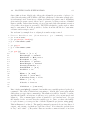
Computational Mechanics featuring Matlab
DRAFT EDITION $Revision: 1.47 $
Richard Sonnenfeld
October 22, 2012
c
2012
Richard Sonnenfeld
Published by: New Mexico Tech Press
All rights reserved
Contents
0.1
0.2
0.3
Introduction – for the student . . . . .
0.1.1 How to read this book . . . . .
0.1.2 Extra credit for corrections! . .
0.1.3 Why computer programming in
0.1.4 Other references . . . . . . . .
Introduction – for the instructor . . .
0.2.1 To the instructor who is new to
0.2.2 Intended audience . . . . . . .
0.2.3 Course design . . . . . . . . . .
0.2.3.1 Lecture portion . . .
0.2.3.2 Lab portion . . . . . .
0.2.3.3 Facilities required . .
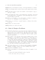
Features of this book . . . . . . . . . .
0.3.1 General features . . . . . . . .
0.3.2 Course timing . . . . . . . . . .
0.3.3 Projects . . . . . . . . . . . . .
0.3.4 Additional topics . . . . . . . .
0.3.5 Chapter by chapter content . .
1 Hello World!
1.1 Steps to “Hello World” . . . . . . .
1.2 “Hello World” . . . . . . . . . . . .
1.3 Getting help . . . . . . . . . . . . .
1.4 Browsing Help . . . . . . . . . . .
1.5 Matlab interactive mode . . . . . .
1.6 Operators and how to calculate . .
1.6.0.1 Exercise 2A . . . .
1.6.0.2 Exercise 2B . . . .
1.6.0.3 Exercise 2C . . . .
1.7 Variables and Memory . . . . . . .
1.7.1 “=” does not mean “Equal”
1.7.2 Variable Types . . . . . . .
3
.
.
.
.
.
.
.
.
.
.
.
.
.
.
.
.
.
.
.
.
.
.
.
.
. . . . . .
. . . . . .
. . . . . .
physics .
. . . . . .
. . . . . .
Matlab or
. . . . . .
. . . . . .
. . . . . .
. . . . . .
. . . . . .
. . . . . .
. . . . . .
. . . . . .
. . . . . .
. . . . . .
. . . . . .
. . . . . . . .
. . . . . . . .
. . . . . . . .
. . . . . . . .
. . . . . . . .
. . . . . . . .
programming
. . . . . . . .
. . . . . . . .
. . . . . . . .
. . . . . . . .
. . . . . . . .
. . . . . . . .
. . . . . . . .
. . . . . . . .
. . . . . . . .
. . . . . . . .
. . . . . . . .
.
.
.
.
.
.
.
.
.
.
.
.
.
.
.
.
.
.
.
i
.
i
.
i
. ii
. ii
. iii
. iii
. iii
. iv
. iv
. iv
. v
. v
. v
. vi
. vi
. vii
. vii
.
.
.
.
.
.
.
.
.
.
.
.
.
.
.
.
.
.
.
.
.
.
.
.
.
.
.
.
.
.
.
.
.
.
.
.
.
.
.
.
.
.
.
.
.
.
.
.
.
.
.
.
.
.
.
.
.
.
.
.
.
.
.
.
.
.
.
.
.
.
.
.
.
.
.
.
.
.
.
.
.
.
.
.
.
.
.
.
.
.
.
.
.
.
.
.
.
.
.
.
.
.
.
.
.
.
.
.
.
.
.
.
.
.
.
.
.
.
.
.
.
.
.
.
.
.
.
.
.
.
.
.
.
.
.
.
.
.
.
.
.
.
.
.
.
.
.
.
.
.
.
.
.
.
.
.
.
.
.
.
.
.
.
.
.
.
.
.
.
.
.
.
.
.
.
.
.
.
.
.
.
.
.
.
.
.
.
.
.
.
.
.
1
1
1
2
3
3
5
6
6
6
6
7
8
4
CONTENTS
.
.
.
.
.
.
.
.
.
.
.
.
.
.
.
.
.
.
.
.
.
.
.
.
.
.
.
.
.
.
.
.
.
.
.
.
.
.
.
.
.
.
.
.
.
.
.
.
.
.
.
.
.
.
.
.
8
8
11
12
12
12
14
14
2 I Will not Throw Massive Projectiles in Class
2.1 Getting homework done quickly with loops . . . . . . .
2.2 Using loops to make a table . . . . . . . . . . . . . . . .
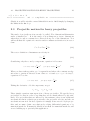
2.3 Projectile motion for heavy projectiles . . . . . . . . . .
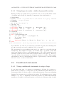
2.3.1 Using loops to make a table of projectile motion
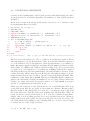
2.4 Conditional statements . . . . . . . . . . . . . . . . . . .
2.4.1 Using conditional statements to stop a loop . . .
2.4.2 Using conditional statements to allow choices . .
2.4.3 Using conditional statements in a while loop . .
2.5 Creating ASCII data files . . . . . . . . . . . . . . . . .
2.6 Logical or Relational operators . . . . . . . . . . . . . .
2.7 More built-in functions . . . . . . . . . . . . . . . . . . .
2.7.1 Checking the size of an error – Absolute value . .
2.7.2 Checking for divisibility – fix() and mod() . . .
2.7.3 Rounding functions . . . . . . . . . . . . . . . . .
2.8 What’s next? . . . . . . . . . . . . . . . . . . . . . . . .
2.9 Review of commands introduced in this chapter . . . . .
2.10 End of Chapter Problems . . . . . . . . . . . . . . . . .
2.11 Code examples for this chapter . . . . . . . . . . . . . .
.
.
.
.
.
.
.
.
.
.
.
.
.
.
.
.
.
.
.
.
.
.
.
.
.
.
.
.
.
.
.
.
.
.
.
.
.
.
.
.
.
.
.
.
.
.
.
.
.
.
.
.
.
.
.
.
.
.
.
.
.
.
.
.
.
.
.
.
.
.
.
.
.
.
.
.
.
.
.
.
.
.
.
.
.
.
.
.
.
.
.
.
.
.
.
.
.
.
.
.
.
.
.
.
.
.
.
.
17
17
18
19
20
20
20
22
23
24
25
26
26
27
27
27
28
29
32
1.8
1.9
1.10
1.11
1.12
1.13
1.7.3 Scientific Notation . . . . . . . . . . . .
Using formatted output . . . . . . . . . . . . .
Combining short scripts . . . . . . . . . . . . .
1.9.1 script and m-file . . . . . . . . . . . . .
A first interactive program . . . . . . . . . . . .
∗
Variables, Memory, and binary codes . . . . .
Review of commands introduced in this chapter
End of Chapter Problems . . . . . . . . . . . .
.
.
.
.
.
.
.
.
.
.
.
.
.
.
.
.
.
.
.
.
.
.
.
.
.
.
.
.
.
.
.
.
3 Arrays, Matrices and Functions
3.1 Arrays and Matrices . . . . . . . . . . . . . . . . . . . . . . . . . .
3.1.1 Arrays . . . . . . . . . . . . . . . . . . . . . . . . . . . . . .
3.1.1.1 Defining and referencing arrays . . . . . . . . . . .
3.1.1.2 Using the diary() function to log your exploration
3.1.2 Row and Column Arrays (1-D Matrices) . . . . . . . . . . .
3.1.2.1 Managing matrices with the size() function . . .
3.1.3 Using Arrays to represent vectors . . . . . . . . . . . . . . .
3.1.3.1 Finding the angle between vectors of arbitrary dimension . . . . . . . . . . . . . . . . . . . . . . . .
3.1.4 Using Arrays to represent sets of measurements . . . . . . .
3.1.5 Comparing vectorized calculations to element-by-element
calculations . . . . . . . . . . . . . . . . . . . . . . . . . . .
3.1.5.1 Initialization . . . . . . . . . . . . . . . . . . . . .
3.1.5.2 Assignment . . . . . . . . . . . . . . . . . . . . . .
3.1.6 More documentation about arrays and matrices . . . . . . .
3.2 User defined functions . . . . . . . . . . . . . . . . . . . . . . . . .
3.2.1 Help on User Defined functions . . . . . . . . . . . . . . . .
35
35
36
36
37
37
38
39
40
40
42
42
42
43
44
45
CONTENTS
.
.
.
.
.
.
.
.
.
.
.
.
.
.
.
.
.
.
.
.
.
.
.
.
.
.
.
.
45
46
47
50
4 Working with Scientific Data
4.1 Working with real data . . . . . . . . . . . . . . . . . .
4.1.1 Reading and Writing Data files . . . . . . . . . .
4.1.1.1 About Metadata . . . . . . . . . . . . .
4.1.2 Working with matrices . . . . . . . . . . . . . . .
4.2 Plotting data with Matlab . . . . . . . . . . . . . . . . .
4.2.1 Basic plotting . . . . . . . . . . . . . . . . . . . .
4.2.2 Improving the appearance of basic plots . . . . .
4.2.3 Saving figures as images . . . . . . . . . . . . . .
4.2.4 Advanced plotting: Objects and handle graphics
4.3 Numerical Derivatives . . . . . . . . . . . . . . . . . . .
4.4 Review of commands introduced in this chapter . . . . .
4.5 End of Chapter Problems . . . . . . . . . . . . . . . . .
4.6 Code examples for this chapter . . . . . . . . . . . . . .
.
.
.
.
.
.
.
.
.
.
.
.
.
.
.
.
.
.
.
.
.
.
.
.
.
.
.
.
.
.
.
.
.
.
.
.
.
.
.
.
.
.
.
.
.
.
.
.
.
.
.
.
.
.
.
.
.
.
.
.
.
.
.
.
.
.
.
.
.
.
.
.
.
.
.
.
.
.
53
54
54
56
56
59
59
60
61
62
65
66
67
74
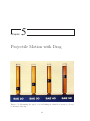
5 Projectile Motion with Drag
5.1 Trajectory and range of a heavy projectile . . . . .
5.2 More Plotting data with Matlab . . . . . . . . . . .
5.2.1 Making publication quality figures . . . . .
5.2.2 Adding authorship information . . . . . . .
5.3 Document, Define, Derive, Display (D4 ) . . . . . .
5.4 Simple animation with Matlab . . . . . . . . . . . .
5.5 Viscosity and Stoke’s Law . . . . . . . . . . . . . .
5.5.1 Defining Viscosity . . . . . . . . . . . . . .
5.5.2 Examples of Viscosity . . . . . . . . . . . .
5.5.3 Two types of viscosity . . . . . . . . . . . .
5.5.4 What causes Viscosity? . . . . . . . . . . .
5.5.5 Stokes’ Law . . . . . . . . . . . . . . . . . .
5.6 Linear Drag in One-Dimension, Terminal Velocity
5.7 Linear Drag in Two Dimensions . . . . . . . . . . .
5.8 Review of commands introduced in this chapter . .
5.9 End of Chapter Problems . . . . . . . . . . . . . .
5.10 Code examples for this chapter . . . . . . . . . . .
.
.
.
.
.
.
.
.
.
.
.
.
.
.
.
.
.
.
.
.
.
.
.
.
.
.
.
.
.
.
.
.
.
.
.
.
.
.
.
.
.
.
.
.
.
.
.
.
.
.
.
.
.
.
.
.
.
.
.
.
.
.
.
.
.
.
.
.
.
.
.
.
.
.
.
.
.
.
.
.
.
.
.
.
.
.
.
.
.
.
.
.
.
.
.
.
.
.
.
.
.
.
81
82
83
84
86
87
88
90
90
91
92
92
93
93
96
96
97
100
6 Quadratic Drag and the Euler Method
6.1 Inertial Drag . . . . . . . . . . . . . . . . . . . . . . . . . .
6.1.1 What causes inertial drag? . . . . . . . . . . . . . .
6.2 Reynolds Number . . . . . . . . . . . . . . . . . . . . . . . .
6.2.1 Fluid mechanics and dimensionless parameters . . .
6.2.2 Reynolds number and drag regimes . . . . . . . . . .
6.3 One-dimensional (1-D) analytic solution for quadratic drag
6.3.1 Hyperbolic functions . . . . . . . . . . . . . . . . . .
.
.
.
.
.
.
.
.
.
.
.
.
.
.
.
.
.
.
.
.
.
.
.
.
.
.
.
.
103
104
104
106
106
107
108
109
3.3
3.4
3.5
3.2.2 Difference between a script and a function
Review of commands introduced in this chapter .
End of Chapter Problems . . . . . . . . . . . . .
Code examples for this chapter . . . . . . . . . .
5
.
.
.
.
.
.
.
.
.
.
.
.
.
.
.
.
.
.
.
.
.
.
.
.
.
.
.
.
.
.
.
.
.
.
.
.
.
.
.
.
.
.
.
.
.
.
.
.
.
.
.
.
.
.
.
.
.
.
.
.
.
.
.
6
CONTENTS
6.4
6.5
6.6
6.7
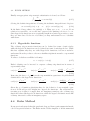
Euler Method . . . . . . . . . . . . . . . .
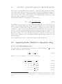
Applying Euler Method to Quadratic drag
6.5.1 One dimensional case . . . . . . .
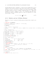
6.5.2 Matlab code for 1-D Euler Method
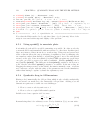
6.5.3 Using sprintf() to annotate plots
6.5.4 Quadratic drag in 2-Dimensions .
6.5.5 Getting position from velocity . . .
End of Chapter Problems . . . . . . . . .
Code examples for this chapter . . . . . .
.
.
.
.
.
.
.
.
.
.
.
.
.
.
.
.
.
.
.
.
.
.
.
.
.
.
.
.
.
.
.
.
.
.
.
.
.
.
.
.
.
.
.
.
.
.
.
.
.
.
.
.
.
.
.
.
.
.
.
.
.
.
.
.
.
.
.
.
.
.
.
.
.
.
.
.
.
.
.
.
.
.
.
.
.
.
.
.
.
.
.
.
.
.
.
.
.
.
.
.
.
.
.
.
.
.
.
.
.
.
.
.
.
.
.
.
.
.
.
.
.
.
.
.
.
.
109
110
110
111
112
112
113
114
117
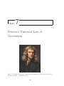
7 Newton’s Universal Law of Gravitation
119
7.1 Introduction . . . . . . . . . . . . . . . . . . . . . . . . . . . . . . . 120
7.1.1 Linear and Angular motion . . . . . . . . . . . . . . . . . . 120
7.2 Newton’s Law of Universal Gravitation . . . . . . . . . . . . . . . . 120
7.2.1 Vector form of Law of Gravitation . . . . . . . . . . . . . . 122
7.3 Kepler’s Laws . . . . . . . . . . . . . . . . . . . . . . . . . . . . . . 123
7.3.1 Introduction . . . . . . . . . . . . . . . . . . . . . . . . . . 123
7.3.2 Planets move in ellipses with the sun at one focus . . . . . 123
7.3.3 Kepler’s Period Law . . . . . . . . . . . . . . . . . . . . . . 124
7.3.3.1 Fictitious forces – What holds the planets up? . . 124
7.3.3.2 Inertial reference frames . . . . . . . . . . . . . . . 126
7.3.3.3 Uniform circular motion . . . . . . . . . . . . . . . 126
7.3.3.4 Orbits in inertial reference frames . . . . . . . . . 128
7.3.3.5 Kepler’s period law for circular orbits . . . . . . . 129
7.3.4 Planets sweep out equal areas in equal times . . . . . . . . 129
7.3.4.1 Rotational form of Newton’s 2nd Law . . . . . . . 130
7.3.4.2 Conservation of Angular Momentum . . . . . . . . 130
7.3.4.3 Equivalence of Kepler’s second law and angular
momentum conservation . . . . . . . . . . . . . . . 131
7.4 Gravitational Potential . . . . . . . . . . . . . . . . . . . . . . . . . 132
7.4.1 Escape Velocity . . . . . . . . . . . . . . . . . . . . . . . . . 133
7.4.1.1 Example: Calculating escape velocity from Earth 133
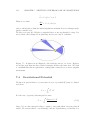
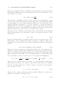
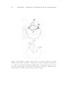
7.5 Gravitation of Extended Bodies . . . . . . . . . . . . . . . . . . . . 134
7.6 Center of Mass . . . . . . . . . . . . . . . . . . . . . . . . . . . . . 137
7.6.1 Example: Calculating center of mass of four point-masses . 137
7.6.2 Correcting Kepler’s period law . . . . . . . . . . . . . . . . 138
7.6.3 Reduced Mass (µ) . . . . . . . . . . . . . . . . . . . . . . . 139
7.6.4 The Bohr Atom . . . . . . . . . . . . . . . . . . . . . . . . . 140
7.7 Review . . . . . . . . . . . . . . . . . . . . . . . . . . . . . . . . . . 142
7.8 End of Chapter Problems . . . . . . . . . . . . . . . . . . . . . . . 142
8 Runge-Kutta Method and Orbital Simulation
8.1 Advantages of higher-order methods . . . . . . .
8.2 First order Runge-Kutta (RK1 or Euler method)
8.3 Second order Runge-Kutta (RK2) . . . . . . . .
8.3.1 RK2 Algebraic Interpretation . . . . . . .
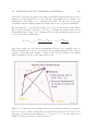
8.3.2 RK2 Graphical Interpretation . . . . . . .
.
.
.
.
.
.
.
.
.
.
.
.
.
.
.
.
.
.
.
.
.
.
.
.
.
.
.
.
.
.
.
.
.
.
.
.
.
.
.
.
.
.
.
.
.
.
.
.
.
.
149
149
151
151
151
152
CONTENTS
8.4
8.5
8.6
8.7
8.8
8.9
Fourth order Runge-Kutta (RK4) . . . . . . . . . . . .
Applying Runge-Kutta methods to quadratic drag . .
Applying Runge-Kutta methods to gravitation . . . .
Sample listing for Runge-Kutta2 applied to gravitation
End of Chapter Problems . . . . . . . . . . . . . . . .
Possible Projects for Physics 241 . . . . . . . . . . . .
8.9.1 Preproposal . . . . . . . . . . . . . . . . . . . .
8.9.2 Proposal . . . . . . . . . . . . . . . . . . . . . .
8.9.3 The Projects . . . . . . . . . . . . . . . . . . .
8.9.3.1 Modeling . . . . . . . . . . . . . . . .
8.9.3.2 Data Analysis . . . . . . . . . . . . .
7
.
.
.
.
.
.
.
.
.
.
.
.
.
.
.
.
.
.
.
.
.
.
.
.
.
.
.
.
.
.
.
.
.
.
.
.
.
.
.
.
.
.
.
.
.
.
.
.
.
.
.
.
.
.
.
.
.
.
.
.
.
.
.
.
.
.
.
.
.
.
.
.
.
.
.
.
.
153
154
157
157
161
168
168
168
168
168
170
8
CONTENTS
0.1. INTRODUCTION – FOR THE STUDENT
0.1
0.1.1
i
Introduction – for the student
How to read this book
In this age of hyperlinks and non-linear thinking, I believe learning can still be
best served by an engaging story that starts at the beginning and progresses
logically to the end. Hyperlinks are good when you are already an expert in an
area and you know just what you are looking for. The story is best when exploring
a world that is new to you; you do not yet know what you are looking for.
While some of the students taking this course may have computer programming
experience, none is expected in advance.
The best way to read a physics (or math, or engineering text) is with pencil and
paper, so that you repeat (or fill in) all the details of derivations and examples
that are given in the book. Psychologists have long known that “active learning”
is the only way to keep your mind engaged in a new and difficult subject. Just
scanning the words on the page is fine for a novel, but not for learning a technical
subject. When the subject is explicitly computer programming, one should have,
in lieu of pencil and paper, an open terminal, or in this case, and open Matlab
command line.
This book in no way tries to be exhaustive in its coverage of the Matlab language
itself. In fact Matlab is huge, and it grows every year. Since it is a commercial
program, it is in the interests of the company that supports it that it should add
features every year. Fortunately, the core language is relatively untouched over
the past 20 years, and I expect it will remain so. This book focuses on the core
language only. It has been my experience in teaching this course that toward
the end, students are comfortable enough with what they need to know that they
can effectively search the extensive on-line and built-in documentation associated
with Matlab.
Because I try to get on with using Matlab for physics as quickly as possible, I
do not have an excessive number of examples of programming concepts. Thus,
it is important that you carefully read each one, and, as suggested, type each
example into the command line (or as a script) as you read. This should leave
you in good shape to do the assigned end-of-chapter problems.
0.1.2
Extra credit for corrections!
What you hold in your hands at the moment is the “Zeroth Edition”. It has
been used to teach a course just once – so it is sure to still be full of typos and
non-sequiturs. Please forgive me. I hope your professor will give you extra credit
if you are the first to e-mail me errors that you find.
ii
0.1.3
CONTENTS
Why computer programming in physics
I teach the class for which this book is designed. Some students are enthusiastic
about the class from the start, but others ask “Why do we need to learn to
program a computer? If I wanted to do that, I would be a CS major.” Here are
my answers to this question.
First, programming can help you learn the physics. Before you can program a
problem, you have to really understand the problem. Debugging the program
when it seems to produce nonsensicial results ALSO helps you learn the physics.
You have to ask yourself repeatedly “What did I expect to happen?” and “What
are test cases that I understand?”. It also enables the solution of many (analytically) intractable problems, from quadratic drag to the orbital motion of multiple
bodies in astrophysics.
Second, computers are now a tool to be used by every scientist and engineer
in the routine pursuit of their work. While many work with professional tools
written by professional programmers, there is often a need for data analysis, or
the application of a simple model in a new area for which no professional tools
exist. If you work in industry, you may have an idea which you can test with a
computer model and learn a lot in a week, or even a day, if you are comfortable
with basic computer programming. New ideas often do not work, at least not
right away, and they are particularly hard to “sell” to your boss, particularly if
you want them to give you budget or assign a programmer to help you test out
your idea. However, if you can test it yourself, you either save embarassment,
or, if successful, help your company take your idea to the next level. If you work
in government or academia, budgets are always tight. Even if you can afford to
hire a programmer, you will give them much better direction if you have tried to
code the problem (however crudely) yourself.
Third, averaging over all parameters of interest, processor speed, memory, harddrive space, and graphics performance; computers have improved by factors of
1000 to 10,000 over the past thirty years. No other aspect of our society has
improved by even a factor of two in the past thirty years. If you do not know
how to fully take advantage of a computer, you are cutting yourself off from the
most incredible advance of our age.
Fourth, CS majors in many cases study computational theory and not its applications to real world problems. Some CS professors no longer even program
themselves. If you came to college with an interest in programming, you might
actually prefer to be a computational physics major, rather than a CS major!
Finally, computer programming is fun. Writing a program is like building a
machine, but it is generally a lot faster and easier than cutting, drilling, screwing,
and soldering.
0.1.4
Other references
There are a plethora of books that aim to teach Matlab, the language, and many
of them do it well, and inexpensively. In this book, I am constantly interleaving
0.2. INTRODUCTION – FOR THE INSTRUCTOR
iii
language instruction with physics so that you the student can always see “the
point” of the new language feature being learned. I find that reading a book
that merely describes the language often leaves beginners unable to bridge the
gap between knowing the language features and using it to solve problems. I
wrote this book carefully so that a student who has read from the beginning
and done the homework will always have the tools they need to do the next
assignment. Still, human brains vary, and some may find it frustrating to have
to leaf through the book to find information on some language feature. To those
I say “use the index”, I included all the commands. If that is not enough feel free
to buy a Matlab specific reference. My view is that the online documentation is
so extensive and of such high quality that a specific reference book is not needed
– you can use the electronic documentation.
0.2
Introduction – for the instructor
I assume the potential instructors have read my messages to the students, so I
will not repeat those.
0.2.1
To the instructor who is new to Matlab or programming
I applaud you for stepping up to the challenge of offering this course. You will
learn a lot. I believe that my text will educate you as well as your students. I
hope you can get three chapters ahead. This ought to provide you with sufficient
buffer to be able to help the students. Clearly, you need to do the homework
problems yourself. Then you will have a good chance of being able to help the
students through their lab periods. My experience, having written the material
and with extensive experience with programming and Matlab, is that task switching between twenty struggling students is still a challenge, so I urge you not to
try to wing it.
During lectures, students often ask questions about the format and capabilities
of various matlab commands. If you do not yourself have this mastered, I recommend an experiential approach. Have a matlab command line projected on a
screen on the side of the classroom. Go experiment with various commands in
front of the class. It will answer their question and will drive home the point
that Matlab is meant to be used interactively in this way. If you are not sure how
something works, experiment! You cannot “break” anything by hacking.
0.2.2
Intended audience
This book is designed for a lower-division physics course with three goals.
1. To give students a second look at the crush of traditional topics presented
in a typical single semester course on classical mechanics.
iv
CONTENTS
2. To give students a first look at the more advanced material and optional material in classical mechanics, such as projectile motion with air-resistance,
fluid mechanics, and center of mass.
3. To teach a programming language, Matlab and to specifically apply it to
the topics of classical mechanics, in hopes that students can carry this new
tool on into more advanced classes and research.
0.2.3
Course design
I have been using pieces of this book for the past four years to teach this course
and so it has been classroom tested. At our school, computational mechanics
was a one semester, 3-unit course with two 50 minute lectures and one two-hour
“lab” or “recitation” per week. It should be emphasized that the “lab” portion
of the course is quite important.
0.2.3.1
Lecture portion
In the lecture portion of the course, I explain concepts and work examples, either
physics examples or programming examples. I used a traditional classroom and
a blackboard. If you have access to a smart classroom with a computer running
matlab and a projector, that would also be good. When I used a projector, I
increased the default font size in the Matlab editor to make it more legible. To
make it easier to go over code details without a projector, I provide, at the end
of the early chapters, a final section called “Code examples used in this chapter”.
This allows you to refer to particular lines of code or constructions in your lecture
without needing to write them rapidly (and usually incorrectly) on the blackboard
and without needing to excessively jump around in the book.
0.2.3.2
Lab portion
This is a hands on course, so the lab is critical, particularly for students with
little/no programming background. This is where students need to get helped
over the first several roadblocks before they begin to become confident that they
can debug their own work. I strongly urge you to run the lab sections yourself,
at least for the first few times that you teach the course. Students make all
sorts of programming mistakes that you cannot imagine until you see them. If
you do not attend the lab yourself, you will be inevitably disconnected from the
real problems your students are having with the programming part of the course.
One year I ran the course with an experienced TA running the labs in my place.
While students survived, the course was less effective than when I ran the lab
myself. The TA was somewhat overwhelmed by the students difficulties.
For each lab, I assign several homework problems and then circulate while the
students work. Sometimes I use a half-hour to demonstrate matlab techniques
(particularly debugging) while students type the same thing at their keyboard. I
do not assign a pre-lab.
0.3. FEATURES OF THIS BOOK
0.2.3.3
v
Facilities required
I used a traditional classroom (chairs, blackboards and no technology) for lectures
and a computer lab (50 desktop computers and 50 monitors with an instructors
workstation and an LCD projector) for labs.
One might imagine teaching the entire course in a computer lab, but I recommend against this. Labs full of desktop computers tend to be noisy, and the
computers are a welcome distraction to the students. Very often computer labs
have inadequate blackboards, and the students are further apart because of the
space taken up by the cmoputers.
The combination of reduced intimacy, noise and distractions result in relatively
ineffective lectures and discussions relative to traditional classrooms.
If you find that you have a computer enabled classroom where students have individual small and quiet computers (e.g. laptops, iPads) and where the instructor
has a tablet which can be projected in real time, you might be able to do all
sessions in it.1
0.3
Features of this book
Before getting to the details of each chapter, the broad features of this book are
as follows:
0.3.1
General features
Universality The goal is to teach programming. Matlab is just a first language.
Over-reliance on Matlab-specific features is avoided.
Physics integration Programming ideas are always tried out on familiar physics.
This reinforces the physics and gives students a handle to hang their programming knowledge on.
Structured programming Before object-oriented programming (OOP), there
was structured programming. Matlab is a fine language for teaching the
structured programming approach (break your jobs up into functions, let
execution proceed in an orderly way from inputs to outputs with as few
tortuous branches as possible, use local variables rather than globals, document what you are doing). Beginners do not have to start with OO abstractions. OOP can be taught once students have some experience under their
belt (and I use Matlab’s “handle graphics” as a way to introduce objects
without going overboard.)
1 Matlab
does not run on an iPad, but since it has always been client/server based, you can
have a window on an iPad to a matlab session running in your computer lab or in the cloud.
vi
CONTENTS
Bias toward the command line Students are raised in a point-and-click world,
and Matlab supports this. You can customize data plots through a GUI
(graphical user interface). I eschew these methods at every turn. Matlab allows programming the appearance of figures and I think it allows for higher
consistency and scientific productivity to write programs to automate, the
analyis, display, and documentation of data rather than encouraging a lot
of handwork on each and every data plot.
New physics Numerical methods can solve many problems that are not solvable
analytically. It is motivating to students to see their new skills put to work
to solve interesting problems.
0.3.2
Course timing
The book is designed in the usual way on the assumption that you will cover
a chapter a week. Experienced instructors know that one sometimes needs to
slow down. In particular, expect to spend 3 weeks on chapter 5/6 together and
another 3 weeks on chapters 7/8. Thus, for a one quarter course, the material
provided is just the right length. For schools on the semester system, this book
is a little short. I know this to be true, and will be adding more material in the
second edition. What I did (and will continue to do in the 2nd edition) is to get
through the 8 chapters in roughly 10 weeks, and then cover other pure physics
topics in class while giving students time to explore the more advanced material
in chapter 8 in labs and to work on independent projects.
0.3.3
Projects
I had students working on these projects for the last several labs, and shifted my
focus to getting them through the homework to getting them to make progress
on their projects. It was quite civilized and allowed for some fairly ambitious
projects. Most of the projects on the list I provide have been attempted and
completed successfully. Some of the best projects were those in which students
came up with their own, sometimes by poking around on Youtube. The descriptions I provide are intentionally pretty broad, and too ambitious in some cases.
Refining a project to something that is achievable in the time given is a skill being
taught via the “deep-end” method. It is your job as instructor to help the student refine/define the project and not drown. My requests for Preproposals and
Proposals were intended to get the students focused on what they could really
achieved. In some cases they worked. There were of course students discovering
in the final days of the course that they had to start over. That is educational
too!
0.3. FEATURES OF THIS BOOK
0.3.4
vii
Additional topics
After covering these 8 chapters, I devoted the last six weeks of the course to three
additional areas: free-body diagrams and dynamics, statics, and collisions in one
and two dimensions. You might choose to cover different areas. These areas
fit nicely in the context of this book and will be included explicitly in future
editions. I did not include them in the first edition because there is such a wealth
of material in other books covering these topics. This course was not intended
as a first exposure to these topics, but rather as a second exposure to allow some
degree of mastery.
0.3.5
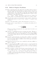
Chapter by chapter content
Here is a summary of the features of each chapter.
Chapter 1 – Hello world! This gets the students started running Matlab, and
introduces the excellent built-in help system immediately. In addition to doing routine arithmetic at the command line, I introduce formatted output.
This may seem an advanced topic, but it gets students thinking about data
formats and types of numbers right away. Even though Matlab is forgiving
about the difference between characters, integers, and floats, pointing out
the difference makes students aware of what is going on inside the computer
and provides them with background useful for any future programming language they might learn.
Chapter 2 – Loops & conditionals We get right to the meat of programming
with for loops, while loops, if statements and boolean logic. Only single
variables (no arrays) are used in this chapter, as I try to provide an approach that will port nicely as students move to other languages. We get
to physics right away, using the familiar equations of projectile motion to
illustrate looping. Conditionals are introduced as a way to figure out when
the projectile has returned to ground (and to stop looping). Output to a
text file is also covered, so that by the end of chapter 2 students can create
data files based on simple equations or sequences.
Chapter 3 – Arrays, Matrices & Functions Arrays are a universal programming construct, and Matlab has particularly powerful array/matrix capabilities. We link to physics by pointing out that a 3-element position or
velocity vector can be represented as an array, then extend to showing that
an array is an excellent way to contain a time-series or other scientific data.
We compare operating on an array element-by-element in a loop to the
parallel array operations built into Matlab. Though Matlab will tolerate
a programmer who does not first declare an array, it is bad practice and
disastrous in other languages. I introduce zeros() as a way to define an
array and think about its needed size. Functions are also introduced, as we
want to get the student learning to break the problem into small chunks
that can be handled by functions. Students write functions to calculate the
viii
CONTENTS
mass of a sphere of known density and the gravitational attraction between
two masses at arbitrary distance. This also allows understanding how to
pass arrays in and out of functions, a subtle concept worth some discussion
in class.
Chapter 4 – Working with scientific data Since students know about arrays, it is time to read files of data and plot it. Labeling your axes and
making your plots self-documenting is emphasized and demonstrated. I
provide data for a weather-balloon flight. Your school doubtless has resevoirs of data that students can practice on. Scientific data is usually
imperfect. It has noise, gaps, missing or corrupted data. It is educational
to see real data as early as possible, and the ability to crunch real data gives
students an employable lab skill. Numerical differentiation is introduced as
an example of a function that is non-trivial.
Chapter 5 – Projectile motion with drag More is said about data plotting
and Matlab’s “handle graphics” features are introduced. The formal DSMV
method (Define, Setup, Model, View) is introduced to encourage students
to view their program as an organized and modular process. Animation is
introduced, both because it is exciting and because it makes the point that
you might have the same data output from your model but want to view
it either as a static plot or an animation. Finally, all of this is applied to
projectile motion with linear drag. Linear drag is analytically solvable, so
students can practice their differential equations and plot something real.
Chapter 6 – Quadratic drag & Euler method Quadratic drag is not mathematically tractable, so it gives an excuse to introduce our first numerical
method for solving differential equations, the Euler method. Despite its
limited accuracy, the Euler method leads students through all the steps of
solving a differential equation numerically. Students use the Euler method
on quadratic and linear drag and can compare their analytical solutions
from the previous chapter with numerical solutions.
Chapter 7 – Gravitation By this time, all the basic programming concepts
students will need have already been introduced. There is no new programming introduced in this chapter. This gives the students time to absorb the
lessons of the first six chapters, and the instructor time to fill in the physics
that will be needed for Chapter 8. We cover all of Kepler’s laws and use
orbital motion as an example of the importance of the center-of-mass frame.
We also use orbits to remind students about angular momentum and potential energy. Finally we derive (by direct integration) the beautiful result
that spherical masses may be treated as point masses. This introduces
spherical coordinates and reinforces calculus.
Chapter 8 – Runge-Kutta method & orbital simulation This is the chapter where all the previous work comes together. The 2nd and fourth-order
Runge-Kutta methods are introduced and explained. The two methods are
applied to quadratic drag, and then RK2 is applied to orbital mechanics.
0.3. FEATURES OF THIS BOOK
ix
The student extends the orbital mechanics model to RK4 for homework,
and is then ready to tackle a variety of problems, from two-body eccentric
orbits to multibody problems and such applications as transfer orbits and
Rutherford scatttering. Students tend to get excited as they realize they
can program a working model of the inner solar system, animate it, and
watch the planets whizzing around. This chapter is the jumping off point
for independent projects (See appendix).
x
CONTENTS
Chapter
1
Hello World!
1.1
Steps to “Hello World”
Brian Kernighan and Dennis Ritchie1 started their famous book on C with a
program that typed “Hello world”. They did this for good reason, because in
C you need to install a “compiler” and a “linker”. You need to write your code
with something called a text editor. Then you needed to compile it, link it, and
finally, run it. So there was a lot of overhead just to get to “Hello world!”.
With Matlab and other modern computing languages like Python life is much
easier. Matlab does not require a compiler or a linker, and it has two modes.
The first is Matlab command line, at which you can just type any single command or group of commands, and they are immediately executed. This is very
helpful for prototyping; about which more will be said later. The second mode
is more like traditional programming languages. It consists of putting a bunch
of Matlab commands into a special file (called an m-file or script). In general,
these commands are executed in the same way as if you had typed them at the
Matlab command line. In what follows, I will call any set of commands in a file
a script. In C, “Hello world” is a six-line program, but in Matlab it is just a one
line script.
1.2
“Hello World”
1. Create and edit the file hello.m with the built-in Matlab editor.
2. Your program consists of just this line:
disp ’Hello World’
1 programming
gods at Bell Laboratories in the 1970s who defined C and also had a lot to
do with Unix
1
2
CHAPTER 1. HELLO WORLD!
3. Save the file hello.m
4. Run the program:
>> hello.m
??? Undefined variable ”hello” or class ”hello.m”.
5. Oops! Leave out the .m
>> hello
Hello World
You just wrote and ran your first program. Congratulations!
1.3
Getting help
Though we have barely begun, it is worth mentioning how to get help in using
Matlab, because its excellent built-in documentation is one of its best features.
Of course there is a web page at http://www.mathworks.com at which you can
look up the full user manual, see many worked examples, and participate in user
forums at Matlab Central. However Matlab predates the web, and so a lot of
support is built into the program itself. It is often far faster to use this built-in
help while hacking away than to go surf the web.
Specifically, there is help at the Matlab command line. For example:
1 >> h e l p l o g
2 LOG
Natural logarithm .
3
LOG(X) i s t h e n a t u r a l l o g a r i t h m o f t h e e l e m e n t s o f X.
4
Complex r e s u l t s a r e p r o d u c e d i f X i s n o t p o s i t i v e .
5
6
See a l s o l o g 1 p , l o g 2 , l o g 1 0 , exp , logm , r e a l l o g .
7
8
R e f e r e n c e page i n Help b r o w s e r
9
doc l o g
Note the definition of log given on line 2 and the extension to complex numbers
given on line 4. Most helpfully, line 6 lists related functions. Surely you can guess
which of these is base 10 logarithm, and of course you could rapidly check your
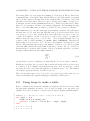
guess by typing help log10. Finally, on line 9 is a reference to the Help browser.
If you try this yourself you will see that the reference is actually a hyperlink to
the local documentation, which provides more detail, and typically examples of
usage of the command.
The main trick in using the command line help is to know the name of the
command you are interested in. Usually you can make an educated guess, and
then See also ... will help you.
1.4. BROWSING HELP
1.4
3
Browsing Help
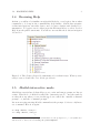
At first, you will not be familiar enough with Matlab to even begin to know what
commands to look up in the command-line help facility. Matlab has extensive
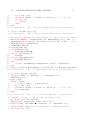
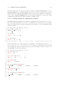
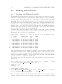
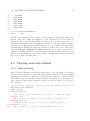
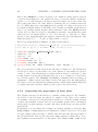
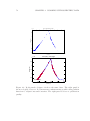
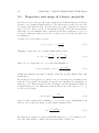
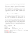
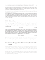
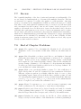
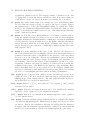
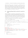
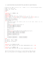
on-line introductions, tutorials, demos, and of course complete and detailed documentation. To begin to use it, either press the F1 function key or select Product
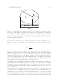
Help from the pull-down menus. You will see screens like those shown in figures
1.1 and 1.2.
Figure 1.1: The Getting Started documentation does what it says. When you are
ready for more detail, the User Guide provides it.
1.5
Matlab interactive mode
Matlab has a special mode that allows you to write and run programs one line at
a time. This mode of Matlab is called the “interactive mode”, and the symbols
>> that show up when you are in this mode are called the “matlab command
prompt”, or just the “command prompt”2
Let us now trying entering Matlab commands at the prompt. So far we only know
one command. Here it is again:
>> disp "Hello, Kitty!"
??? disp "Hello, Kitty!"
|
2 “Prompt”
is another computing word. In Windows, the prompt is C:\ > or C:\Windows>
and in Linux or Darwin it is something like you@computer:
4
CHAPTER 1. HELLO WORLD!
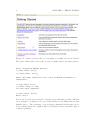
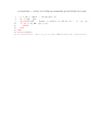
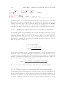
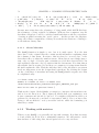
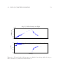
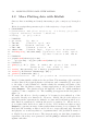
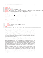
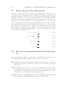
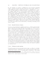
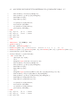
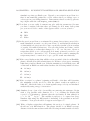
Figure 1.2: Getting Started tells you everything you might need about Matlab.
The point of this textbook is to tell you why you might want to use these features.
Error: Unexpected MATLAB operator.
>> disp "Hello, Kitty"
??? disp "Hello, Kitty"
|
Error: The input character is not valid in MATLAB statements or
expressions.
>> disp "Hello Kitty"
??? Error using ==> disp
Too many input arguments.
>> disp ’Hello, Kitty!’
Hello, Kitty!
Note I used double quotes instead of single-quotes and thus got three different
error messages! Computers are notoriously finicky about things that normal
humans ignore. The advantage of prototyping commands in interactive mode
before putting them into scripts is that you rapidly fix these inevitable slips of
computer grammar.
1.6. OPERATORS AND HOW TO CALCULATE
5
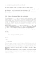
We can also print the results of a calculation. Here is a simple example:
>> fprintf(’The answer to life, the universe and everything is %d.\n’,6*7)
The answer to life, the universe and everything is 42.
The example above demonstrates formatted output which will be discussed further in section 1.8.
1.6
Operators and how to calculate
The familiar symbols +, −, ×, and ÷ are referred to by the fancy name of “mathematical operators”, or just “operators”. Of course, Matlab includes other functions you would expect, such as exponentials, and logarithms (as mentioned in
section 1.3). Trigonometric functions are accessed as you would imagine, sin(x),
csc(x), etc.. Further, there are other, less common operations in Matlab that
are still quite useful. So “operators” is a useful piece of vocabulary to add to our
hacking jargon.
In most computer languages, +, −, ×, and ÷ are replaced by +, −, ∗, and /. The
∗ is used for multiplication because × is too easy to confuse with the variable
“x”. The / is used for division because few computer keyboards include a ÷.
You can do calculations directly at the Matlab “prompt”. Follow along at your
computer as we do so:
>> 2**3
??? 2**3
|
Error: Unexpected MATLAB operator.
>> 2^3
ans =
8.0000e+000
Note again the error message for 2**3. In this case Matlab did not recognize the
operator **. It does recognize *, however, so the error statement shows a vertical
line pointing at the second star. Matlab tries to be as specific as possible about
what it does not understand to try to help you recognize the error and fix it.
Having√fixed our error, we can notice that "2^3" means 23 , and that 3^(0.5)
means 3.
From math classes you know about “order of operations”. The order of operations
in computer programming are the same as in mathematics. Just as in math, if you
find a particular formula ambiguous, use parenthesis to clarify. See the examples
in the exercises below.
6
1.6.0.1
CHAPTER 1. HELLO WORLD!
Exercise 2A
What is the surface area of the Earth?
>> 4*pi*6400E3^2
5.14e+014
1.6.0.2
Exercise 2B
There are 99 bottles of beer on the wall. Each bottle contains 16 ounces. Before
you arrived, someone took 9 bottles down, and passed them around. There are
currently 74 people at the party. Assuming all share equally, how many ounces
does each person get of the remaining beverage?
>> (99-9)*16/74
19.4595
1.6.0.3
Exercise 2C
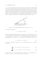
A projectile is launched with an initial speed of 25 m/s at an angle of 30◦ above
horizontal. What is its component of velocity parallel to the ground?
>> 25*cos(30*pi/180)
21.6506e+000
Note that no parentheses were needed in Exercise A because exponentiation occurs before multiplication. Note also that π is built into Matlab. Finally, note
that the cos() function we used just above expects angles to be expressed in
radians. You can easily convert degrees to radians as we did, or you can use the
alternate functions cosd() and sind(), which accept arguments in degrees.
1.7
Variables and Memory
You can also assign the result of a calculation to a variable. Computer languages
like Matlab use variables much like they are used in algebra, except that computer
variables can (and usually should) have names that are longer than just a single
letter.
1 >> x=3+4;
2 >> d e l t a X =3∗5−1
3 deltaX =
4
1 4 . 0 0 0 0 e +000
5
1.7. VARIABLES AND MEMORY
6
7
8
9
10
11
12
13
14
15
16
17
18
19
20
>> c u b e o f 2 =2ˆ3;
>> y =2ˆ4;
>> [ x , d e l t a X ]
ans =
7 . 0 0 0 0 e +000
7
1 4 . 0 0 0 0 e +000
>> y
y =
1 6 . 0 0 0 0 e +000
>> z=x+y−3∗ d e l t a X
z =
− 1 9 . 0 0 0 0 e +000
Notice that the results of the calculations were assigned to variables, then the
values of these variables were printed just by typing the name of the variable.
Why was the value for deltaX on line 3 printed right away, but for y on line 9
you had to again type y on line 12? Matlab makes debugging easy by giving you
the value of any variable as soon as it is assigned or changed. This is often not
what you want, though, so you can suppress this printout by adding a ”;” to the
end of the line.
Computers have “memory”, which is where all the numbers used in any program
are kept. For example, on line 1: x=3+4. The numbers 3 and 4 are in memory,
and line 1 tells the computer to calculate their sum and stick it in another part of
its memory. It names that part of its memory “x”, so when you use “x” later in
the program, the computer checks its memory and fetches the number you saved.
Notice also the statement on line 17: z=x+y-3*deltaX. The computer has already put numbers in memory locations called “x”, “y”, and “deltaX” from the
statements on previous lines. It fetches the numbers back, does the calculation,
and puts the result in a new memory area “z”. This is really all you need to
know about how variables work, but it is a fascinating subject, and if you want
to know more about variables and memory, read section 1.11.
1.7.1
“=” does not mean “Equal”
The meaning of the equal (=) sign in computing is similar but not identical to
that in mathematics. This is most clearly illustrated with the statement x=x+1.
In math, you would “solve for x” and discover that there were no values of x
to satisfy the equation. In computing, the convention is that this statement is
interpreted beginning to the right of the “=” sign. The value in x is retrieved, the
number 1 is added to it, finally the result is assigned back in the memory location
labeled by x. For this reason, “=” is sometimes referred to as the assignment
operator. For more details, see Section 1.11.
8
1.7.2
CHAPTER 1. HELLO WORLD!
Variable Types
We just said that variables are locations in memory where numbers are kept.
Computers tend to distinguish between different kinds of numbers. In Matlab,
the three most important kinds of variable are “integer”, “float”, and “string”.
Integers in computing are defined as in math. They correspond to the whole
numbers, and do not have decimal points. Thus -72, 3, and 11348934432 are
integers, but 1.0 is not. Floating point numbers, or “floats” correspond to the
“real numbers”3 in math class. Floats can be recognized by their decimal points.
The number 1.000 is a float, as is 22.44572435. The computer actually saves
floats in memory in a different format than integers. Languages like C take all
this very seriously. Matlab is a bit more casual about it, but it is important to
know the difference now, as you will likely use other languages in your career that
are more “strongly typed”. With Matlab you can mostly ignore the difference
between integers and floats, but it is worth knowing that there is a difference,
and it can sometimes be important. (For example, Matlab array subscripts must
be integers, and you will get an error if you use a float. We will talk about arrays
later!)
“Strings” are stored in memory as integers, but when either printed or used in
calculations, these numbers are interpreted as letters.4 One character strings are
‘a’, ‘D’, ‘&’, ‘(’, ‘8’, etc. You can make sequences of one character strings, like
‘Hello world’.
In summary ’42’, the string, 42 the integer and 42.0 the float are all stored
differently by the computer.
1.7.3
Scientific Notation
While discussing floats, we should mention that Matlab has scientific notation
built in. We already used scientific notation in example 1 for the radius of the
Earth. In 2004, Cornell scientists weighed a single E-coli bacterium. Its weight
was 6.65 femtonewtons, or 6.65 × 10−15 N . In Matlab this number is written as
either 6.65E-15 or 6.65e-15.
1.8
Using formatted output
Here are some examples of scientific calculations with Matlab. You can either
prototype this code by typing it a line at a time at the Matlab prompt, or you
can use the Matlab editor to create a file called ly.m that contains the following
3 To be more precise, floats correspond to the “rational numbers” in math. Remember that
rational numbers have a finite number of decimal places, or can be expressed by a fraction of
two integers. Real numbers can have an infinite number of decimal places. Clearly a computer
cannot store an infinite number of decimal places. In practice, Matlab works with up to 16 digits
of precision.
4 See section 1.11 for examples of how numbers are interpreted as letters.
1.8. USING FORMATTED OUTPUT
9
lines: (Note: Either way you do it, you can omit typing lines 1-5, 9, and 12. Lines
that start with a % are called “comments” and are there to provide information
for the programmer. They are extremely important for your future programming
success, but the computer ignores all these lines. It as if they were blank.)
1
2
3
4
5
6
7
8
9
10
11
12
13
14
15
16
17
18
%DOCUMENT
%s c r i p t l y .m
%C a l c u l a t e s t h e number o f m e t e r s i n a l i g h t y e a r
%USAGE :
>> l y
%DEFINE
c = 2 . 9 9 7 9 2 4 5 8 E8 ; % s p e e d o f l i g h t i n m/ s
s e c s p e r h o u r =3600;
days per year =365.25;
%DERIVE
s e c s p e r y e a r=s e c s p e r h o u r ∗24∗ d a y s p e r y e a r ;
l i g h t y e a r=c ∗ s e c s p e r y e a r ;
%DISPLAY
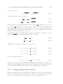
f p r i n t f ( ’ There a r e %f m e t e r s i n a l i g h t y e a r \n ’ , l i g h t y e a r )
f p r i n t f ( ’ There a r e %e m e t e r s i n a l i g h t y e a r \n ’ , l i g h t y e a r )
f p r i n t f ( ’ There a r e %10.2 e m e t e r s i n a l i g h t y e a r \n ’ , l i g h t y e a r )
f p r i n t f ( ’ There a r e %13.2 f m e t e r s i n a l i g h t y e a r \n ’ , l i g h t y e a r )
f p r i n t f ( ’ There a r e %10.0 f m e t e r s \ t i n a l i g h t y e a r \n ’ , l i g h t y e a r )
f p r i n t f ( ’ There a r e %x m e t e r s i n a \ t l i g h t y e a r \n ’ , l i g h t y e a r )
Lines 13-18 introduce a more general and powerful way to display numerical
results. After fprintf(), you can type whatever text you like, 5 There is something
new in this string; constructs such as %f, %e, %10.2f, or %x. (These new things
are collectively called “format control characters”). Following the string and the
format control characters is a comma, and then a variable. The output of these
fprintf() statements should suggest how it all works.
1
2
3
4
5
6
There
There
There
There
There
There
are
are
are
are
are
are
9460730472580800.000000 meters i n a l i g h t y e a r
9 . 4 6 0 7 3 0 e+15 m e t e r s i n a l i g h t y e a r
9 . 4 6 e+15 m e t e r s i n a l i g h t y e a r
9460730472580800.00 meters i n a l i g h t y e a r
9460730472580800 meters
in a lightyear
9 . 4 6 0 7 3 0 e+15 m e t e r s i n a
lightyear
The % expression is replaced by the value of whatever variable follows the comma.
(We just saw the % character used to represent a comment, but this use is
different.) The general name for this is “formatted output”.
Some of the
formatting characters, and their uses, are tabulated below. It should be noted
that fprintf() in Matlab is almost identical to printf() in C. Likewise, this
entire section on control characters and formatted output carries almost without
alteration directly over to C, Java, Fortran, Python, and several other languages.
5 Programmers
often call a group of letters used like this in code a text string or just a string.
10
CHAPTER 1. HELLO WORLD!
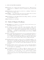
Letter
Meaning
Use
g,G
e,E
f
General
Exponential
Fixed point
i,d
o
x,X
s
c
Decimal
octal
hex
string
char
Matlab chooses best way to show the number
Number is shown in scientific notation, even if it is “2”
Number shown with no exponent but with
fixed number of decimal places
Integer or decimal notation
Integer - in base 8
Integer - in base 16
String - for printing groups of letters
Character - for printing single letters
Table 1.1: Format control characters for displaying numerical or character results
in different ways. For further details, type >> help fprintf.
The \n is also a special control character. It tells fprintf() to skip to the next
line. Try leaving it out and see what happens! Another useful control character
is \t which inserts a tab. You can see its effect on lines 5 and 6 of the output.
Line 15 of the script contains %10.2e. The number 10.2 means leave 10 spaces
for the answer. You can see the effect of the 10 spaces on line 3 of the output.
The number itself only takes up 8 spaces, so two blank spaces are left before it.
This .2 after the 10 means to show two decimal places in scientific notation. On
line 16, %13.2f means show two decimal places after the decimal point, but do
not use scientific notation. Again the 13 means allow 13 spaces. Note on line
4 of the output that the answer actually takes up 19 spaces. Matlab pads short
numbers with spaces, but if the number is longer than the space requested, it
still shows the entire number.
In section 1.6, you did some basic calculations with Matlab. Now you can do
calculations that use variables to make the calculations clearer. You can also
use fprintf() statements to create output that explains the result instead of just
giving a number. Try these exercises, then look at the solutions to see how to
use variables and fprintf() statements to make each calculation very clear.
Ex. 1-A — Two spherical students are sitting 50 centimeters apart. What is
the force of gravitational attraction between them? Assume one student weighs
120 pounds and the other 180 pounds.
Answer (Ex. 1-A) — 1.19 ×10−6 N
1
2
3
4
5
%s c r i p t s t u d e n t A t t r a c t i o n .m
%C a l c u l a t e s the a t t r a c t i v e f o r c e
%USAGE :
>> s t u d e n t a t t r a c t i o n
G=6.673E− 1 1 ; %mˆ 3 / k g s ˆ 2
m1= 1 2 0 ∗ 0 . 4 5 3 6 ;
b e t w e e n two
students
1.9. COMBINING SHORT SCRIPTS
11
6 m2= 1 8 0 ∗ 0 . 4 5 3 6 ; % 4 5 3 . 6 g / p o u n d
7 r =0.5;
8 F=G∗m1∗m2/ r ˆ 2 ;
%N e w t o n ’ s U n i v e r s a l l a w o f g r a v i t a t i o n
9 f p r i n t f ( ’ S t u d e n t m a s s e s a r e %4.1 f and %4.1 f kg . ’ ,m1 , m2)
10 f p r i n t f ( ’ S t u d e n t s e p a r a t i o n i s %3.1 f m. \n ’ , r )
11 f p r i n t f ( ’ I n t e r s t u d e n t a t t r a c t i v e f o r c e i s %5.2 e N. \n ’ , F ) ;
Ex. 1-B — How small would the friction coefficient of the student with the
ground need to be for the students to slide together owing to their gravitational
attraction to one another?
Answer (Ex. 1-B) — µ <2.22×10−9
1
2
3
4
5
6
7
% s c r i p t miniMu .m
%C a l c u l a t e s the f r i c t i o n c o e f f i c i e n t to a l l o w s t u d e n t c o a l e s c e n c e .
%USAGE :
>> m i n i M u
studentAttraction ;
g =9.8;
mu=F / (m1∗ g ) ;
f p r i n t f ( ’ F r i c t i o n c o e f f i c i e n t n e e d s t o be < %5.2 e . \n ’ ,mu ) ;
1.9
Combining short scripts
Note that Exercise 1-B made use of exercise 1-A. This is the first example of
a very powerful programming technique which we will use extensively. Rather
than write one long script, it is often much more productive to write several short
scripts, debug them individually, and then combine them. The script miniMu.m
in its first line of code calls the script studentAttraction.m. The power in this is
that miniMu does not need to recalculate the force of attraction between students,
it can use the result already calculated by studentAttraction.
Some more explanation is needed about why this works. In Matlab, ordinary
scripts, which are just lists of Matlab commands, can share variables with eachother and are available to you at the Matlab command line. A new computing
definition is in order. Variables that may be shared between multiple programs
without any special effort are called global in scope. The power of global variables
comes at a cost, which will be discussed later. Suffice it to say that not all variables in Matlab are global. If a script starts with the special command function,
then its variables are only valid inside itself. They are called local variables. We
will discuss more about global and local variables, as well as workspaces later.
12
CHAPTER 1. HELLO WORLD!
1.9.1
script and m-file
All the files we will create to use in matlab end with .m . In this chapter, the
terms script and m-file are synonomous. In the next chapter we will see that
there is a second common type of m-file called a function.
1.10
A first interactive program
Section 1.2 told you how to run the same script more than once. However, if you
get the same result every time it is not interesting!
With one more command, input we can write a program that it worth running
more than once, even if it is not fascinating. Google will tell you that a furlong
per fortnight is the same as 0.000166 m/s. Likewise 1 mile per hour is 0.447 m/s.
So we can write a script to convert speed in miles per hour to speed in furlongs
per fortnight.
1 %S c r i p t : f u r l o n g s .m
date : 2009/08/20
author : Sonnenfeld
2 meter per s to fur per fort conversion = 0.000166309;
%m/ s
3 mph to meter per s conversion = 0.44704 ;
%m/ s
4 mph to fur per fort conversion = . . .
5
mph to meter per s conversion / meter per s to fur per fort con
6 mph speed=i n p u t ( ’ P l e a s e e n t e r your s p e e d i n m i l e s p e r hour \n ’ ) ;
7 f u r f o r t s p e e d=mph speed ∗ m p h t o f u r p e r f o r t c o n v e r s i o n ;
8 f p r i n t f ( ’ Your s p e e d i s %6.1 f f u r l o n g s p e r f o r t n i g h t \n ’ , f u r f o r t
Note that input allows the user to enter a number, and gives them a message
telling them what to enter. Try running this program a couple of times, entering
different numbers. Now try entering some text instead of a number. You will
see that Matlab gives an error message because it, like most computer languages,
treats text and numbers differently.
1.11
∗
Variables, Memory, and binary codes
We consider again a simple expression like: x=3+4. Here is what the computer is
actually doing:
1. Move the binary number 0011 (3) from memory to the ALU6
2. Move the number 0100 (4) from memory to the ALU
3. Execute the instruction add, and get 0111 (7).
4. Stick this result in a new location (“address”) in memory.
6 ALU
– Arithmetic Logic Unit
1.11.
∗
VARIABLES, MEMORY, AND BINARY CODES
13
5. Use the letter “x” as a shortcut for this “address”.
If this seems slow, remember that each of the steps above takes place in the
time of one cycle for the microprocessor (approximately). For a “slow” 1 GHz
processor, a cycle is a nanosecond, so the above statement could be completed in
5 nanoseconds.
As you may have heard, inside a computer there really is nothing but numbers.
The pictures that we love are encoded as numbers, and there are numerical codes
that are converted to text characters. For example in ASCII7 The letter Q
corresponds to the decimal number 81 or the hexadecimal number 8 51 or the
binary number 01010001.
To translate from binary (base 2) to decimal in your head, add the appropriate
power of two for every digit in a binary number that is a “1”, and ignore every
“0”. It is just a “place-holder” (the same as in base 10).
For example: 112 means 21 + 20 = 2 + 1 = 3.
Another example: 101102 means 24 +22 +21 = 16 + 4 + 2 = 22.
You have probably figured out by now that the subscripted 2 is a way of clarifying
the base so that you know that 112 means “three”, while 11 means “eleven”.
The electrical engineers at New Mexico Tech wear the following T-shirt: “There
are only 10 kinds of people. Those that know binary, and those that do not.”
Enough said!
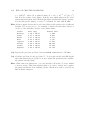
Ex. 1 — Write the binary numbers from 1-16
Ex. 2 — Convert to base 10: 1012
Ex. 3 — Convert to base 10: 101012
Ex. 4 — Convert: 111012
Ex. 5 — Convert: 10100012
Answer (Ex. 1) — 1, 10, 11, 100, 101, 110, 111, 1000, 1001, 1010 1011, 1100,
1101, 1110, 1111, 10000
Answer (Ex. 2) — 5
Answer (Ex. 3) — 21
Answer (Ex. 4) — 29
Answer (Ex. 5) — 81
7 ASCII
– American Standard Code for Information Interchange
or “hex”, is base 16 – we’ll discuss!
8 hexadecimal,
14
CHAPTER 1. HELLO WORLD!
1.12
Review of commands introduced in this chapter
For more information on each command type >>help cmdname at the Matlab
command line.
cos() Cosine of argument in radians.
disp() disp(X) displays variable X without printing its name. Otherwise it is
same as leaving the semicolon off and typing X. If X is a string, the text is
displayed.
input() Prompt for user input.
fprintf() Write formatted data to text file.
%s, %d, %e, %i Formatting strings. Strangely, Matlab help refers you to a C
manual for these.
strings Character strings, arrays of text (help strings).
log() Natural logarithm.
+, -, *, /, ^ Arithmetic operators (help arith).
types of numbers Matlab has integers, floats, and strings, (and variations on
these)(help datatypes).
1.13
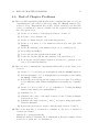
End of Chapter Problems
(1) The universe is about 15 billion years old. The radius of the observed universe is 15 billion light-years. Using this fact and the observation that
there are only about one million atoms in every cubic meter of space (on
average), write a script to calculate the total number of atoms in the universe. Use a fprintf() statement to give your numerical answer with a
complete sentence. [The result of this calculation, by the way, is about the
largest possible number that represents a number of objects. There are
many larger numbers used in mathematics and science, but they represent
ideas or probabilities, not real things.]
(2) In England and Ireland people still give their weight in “stones”. Write an
interactive script that asks you your weight in pounds and tells you your
weight in stones.
(3) Write an interactive script that first asks you the speed of a projectile, then
the launch angle in degrees, and returns to you the x and y components of
the velocity, as follows:
Launch angle = 30◦ , speed=10 m/s, vx= 8.6 m/s, vy=5 m/s
1.13. END OF CHAPTER PROBLEMS
15
(4) Write an interactive script that first asks you your name, then asks you your
weight, then tells you roughly how many moles of hydrogen, oxygen and
carbon you contain. You can approximate that the human body is 75%
water by weight, and the rest is carbon. The output of the script should
include your name and atomic composition. For example:
Hello Richard, you contain 7,500 moles of hydrogen, 3750 moles of
oxygen and 1875 moles of carbon.
hint #1 By default, the input() command expects you to enter a number. If
you want to enter text, you need to use the alternate form of input()
which allows the entry of strings. Matlab will explain it to you if you type
>> help input .
hint #2 Among other things, you have been asked to print back the name of the
user using fprintf(). To print text in Matlab (and many other computer
languages), you use the %s format control sequence (refer to Table 1.1
above
hint #3 In case you forgot how moles work, a mole of (for example) Helium
weighs four grams, because the atomic weight of Helium is four Atomic
Mass Units (AMU).
16
CHAPTER 1. HELLO WORLD!
Chapter
2
I Will not Throw Massive
Projectiles in Class
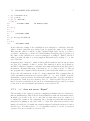
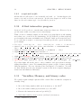
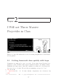
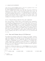
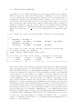
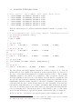
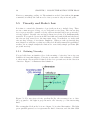
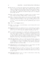
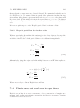
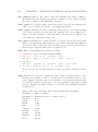
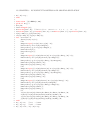
Figure 2.1: Jason Fox makes short work of a writing assignment in C, but Matlab
is even quicker!
2.1
Getting homework done quickly with loops
Computers are supposed to save you work. Notice that Jason Fox has been
assigned to write “I will not throw paper airplanes in class”, five hundred times.
Naturally, he found a way to have the computer save him a lot of tedious work.
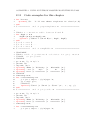
Let us see how to do that. We need the programming concept of a “loop”.
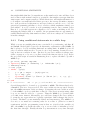
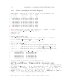
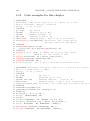
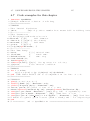
1 f o r k =1:10
2
f p r i n t f ( ’%i .
I ’ ’ l l n o t throw a i r p l a n e s i n c l a s s \n ’ , k )
3 end
4 % ========== e n d o f p a p e r a i r p l a n e s . m ================
17
18CHAPTER 2. I WILL NOT THROW MASSIVE PROJECTILES IN CLASS
Try saving this code as a script and running it. Next type it line by line at the
commmand line. You will see that Matlab will not come back with a >> prompt
after you have entered the first line at the command line. It will not come back
after the second line either. However, once you have typed end to end the loop,
it will spit out the ten line punishment all at once. That’s a big time saver! Three
lines of code generated ten lines of a writing assignment. Try changing the first
line to for k=1:200, and you will see you have become even more efficient!
This illustrates loops, another universal programming construct. We will dissect
the first line of code: for k=1:10. This line can be read aloud as follows: For k
runs from one to ten. The variable k is often called the loop index or the loop
counter. The number 1 is the lower limit or initial value of the loop, while the
number 10 is the upper limit or final value. As you might imagine, the loop
counter could be called anything, x, index, jane, voldemort. Likewise the
initial value does not need to be 1. It can be any number, and need not be an
integer. After the for, there can be any number of lines of code. The loop must
end with end, which tells Matlab that it should go back to the top of the loop,
increment the loop index, and continue. Given your math experience, you have
perhaps realized that for k=1:200 is similar to:
k=200
X
k
(2.1)
k=1
except that you can do anything you want with k. You do not have to sum it.
Finally we note that, the loop can count down as well as up, and it does not need
to count by 1. For example, the statement for k=3:-0.1:1.2 sets k to 3, then
decreases it by 0.1 every time through the loop until it gets to 1.2. The number
-0.1 in the previous sentence is called a step size.
The concepts and terms of loop, loop index, lower limit, upper limit, and step size
exist in essentially all computer languages, including C and Python.
2.2
Using loops to make a table
Before computers and electronic calculators, engineers did their jobs by looking
up important quantities in tables. A loop lets you make your own table very
quickly. Let’s say you want to convert between degrees Celsius and Fahrenheit.
1
2
3
4
5
6
7
8
%M a k e s a c o n v e r s i o n t a b l e b e t w e e n C a n d F .
f o r degC = 0 : 6
degF = ( 9 . 0 / 5 . 0 ∗ degC ) + 3 2 ;
f p r i n t f ( ’%2d C = %4.1 f F\n ’ , degC , degF )
end
% 0 C = 32.0 F
% 1 C = 33.8 F . . .
2.3. PROJECTILE MOTION FOR HEAVY PROJECTILES
9 % 6 C = 42.8 F
10 % ========== e n d
of
tempTable .m
19
=====================
Clearly, it would be trivial to extend this table from 0 to 100 C simply by changing
the limits in the for loop.
2.3
Projectile motion for heavy projectiles
The study of projectile motion can also be called “Two-dimensional kinematics
under constant force”. It is the study of how things move in two dimensions
when there is only a constant force directed along one of the dimensions. You
will recall that the equation for motion under constant acceleration is, in vector
form:
1
~r = ~r0 + ~v0 t + ~at2
2
(2.2)
The vector definition of instantaneous velocity is:
~v =
d~r
dt
(2.3)
Considering only the x, and y components, equation 2.2 becomes:
1
x = x0 + v0x t + ax t2
2
1
y = y0 + v0y t + ay t2
2
(2.4)
Where we have taken positive y to be upwards and where the constant acceleration due to gravity is directed down. Since ax = 0 and ay = −g = −9.8 m/s2 ,
equations 2.5 become
x = x0 + v0x t
1
y = y0 + v0y t − gt2
2
(2.5)
Taking the derivative of both components, we get
vx = v0x
vy = v0y − gt
(2.6)
These simple equations sum up motion of heavy projectiles. We specify heavy
projectiles of course in order to say that they are not much affected by air resistance. For projectiles that are affected by air-resistance, there is an additional
acceleration term in y that is proportional to the projectile velocity, and also an
acceleration term in x. In fact, equation 2.2 simply is incorrect for light projectiles, and we must obtain our solutions by solving differential equations or by
numerical methods. Fortunately Matlab is excellent for numerical methods, and
we are building up to precisely this application.
20CHAPTER 2. I WILL NOT THROW MASSIVE PROJECTILES IN CLASS
2.3.1
Using loops to make a table of projectile motion
Having recalled our equations for projectile motion, we can readily make a table
of position and velocity for just the y-component of projectile motion.
1
2
3
4
5
6
7
8
9
10
11
12
13
14
15
16
17
18
19
%DOCUMENT
%M a k e s t a b l e o f p o s i t i o n s & v e l o c i t i e s f o r p r o j . m o t i o n
%USAGE :
>> p r o j e c t i l e
%DEFINE
g= 9 . 8 1 ; %g i n m/ s ˆ 2
y0 =10; %m
v0y =22; %m/ s
f p r i n t f ( ’ Time \ t V e l o c i t y \ t
A l t i t u d e \n ’ )
f p r i n t f ( ’ sec \t
m/ s
\t
m
\n ’ )
f p r i n t f ( ’==== \ t ======== \ t ======== \n ’ )
%DERIVE
timestep =0.2;
f o r t =0: t i m e s t e p : 1 0
y = y0 + v0y ∗ t − ( 1 / 2 ) ∗ g ∗ t ˆ 2 ;
vy = v0y− g ∗ t ;
%DISPLAY
f p r i n t f ( ’ %4.1 f \ t %6.1 f \ t %7.1 f \n ’ ,
t , vy , y )
end
% ========== e n d o f p r o j e c t i l e . m ====================
Note that line 13 of the above script uses a variable step size, incrementing time
t by 0.2 seconds on every loop instead of by one second.
The program above gives altitude and speed vs. time for a projectile thrown
straight up. How might one figure out at what time a projectile would land
given some initial velocity vy0 and displacement y0 ? We could certainly solve the
quadratic equations in 2.4 for the time at which y takes on the value y0 . However,
once the effects of air-resistance are included equation 2.4 will no longer apply
and might not allow for an analytical solution. A general way to find the landing
time is to use a conditional statement.
2.4
2.4.1
Conditional statements
Using conditional statements to stop a loop
A very important part of computer programming is allowing the computer to
make choices of what to do next based on the calculations it has already done.
Statements which do this are called conditional statements. Every programming
language known supports a conditional execution. Most languages use a syntax
similar to “if – else ” to implment conditional execution. Conditional statements
usually need logical (or relational) operators. (Section 2.6 discusses what a logical
2.4. CONDITIONAL STATEMENTS
21
operator is and explains many of the logical operators that Matlab supports. Once
you read section 2.6, you will see that there are a number of other logical operators
available.)
Below is an excerpt from the projectile script of section 2.3.1, to which a conditional statement has been added.
1
2
3
4
5
6
7
8
9
10
11
12
13
14
15
g= 9 . 8 1 ; %g i n m/ s ˆ 2
y0 =10; %m
v0y =22; %m/ s
f p r i n t f ( ’ Time \ t V e l o c i t y \ t
A l t i t u d e \n ’ )
f p r i n t f ( ’==== \ t ======== \ t ======== \n ’ )
timestep =0.2;
f o r t =0: t i m e s t e p : 1 0
y = y0 + v0y ∗ t − ( 1 / 2 ) ∗ g ∗ t ˆ 2 ;
vy = v0y− g ∗ t ;
f p r i n t f ( ’ %4.1 f \ t %6.1 f \ t %7.1 f \n ’ ,
t , vy , y )
i f ( y < 0)
break
end
end
% ========== e n d o f p r o j e c t i l e B r e a k . m ===============
Lines 11-13 are the added code. The < on line 11 is a relational operator. Every
time through the loop, the if statement on line 11 is executed and the expression
y < 0 is evaluated. If y is less than zero, then the statement y < 0 evaluates to
true. (In many computer languages, including Matlab, true is a built in variable
with a value of 1. false is also built in, and has a value of 0). If y is greater than
or equal to zero, the expression y < 0 evaluates to 0 (false). When a the condition
following an if is true, the lines immediately following the if are executed. If the
condition is false, all the lines between if and the next end are skipped. In the
script at hand, there is only one line to execute between the if and the end. That
command on that single line is break. The keyword break tells the computer to
jump to the statement following the endand to stop looping. This is exactly the
behavior we want. Our table is generated until y < 0, then break is executed
and the loop which generates the table stops.
Please type the script above into Matlab and see for yourself that the table stops
on the first point after the projectile is lower than zero altitude. Having verified
that the script works, change line 2 so that y0 = −10 instead of y0 = 10? Run
the script and notice that the table stops printing after the first line. Why? Of
course we started our projectile with y < 0, so now the condition is true immediately. Our code is working properly. It is our logic that is incorrect. What we
really want is to stop the script once the projectile gets below 0 if it is falling. We
can easily check if it is falling by also checking that vy < 0. It is only necessary
to change line 11 of the script as follows:
if
( y < 0 ) && ( vy < 0 )
22CHAPTER 2. I WILL NOT THROW MASSIVE PROJECTILES IN CLASS
% ==========
end
of
projectilebreakexcerpt
==========
The above conditional is only true when both y < 0 and vy < 0. This demonstrates that you can check more than one condition in a single if statement.
2.4.2
Using conditional statements to allow choices
Conditional statements (if commands) are broadly useful to programmers. For
example, conditional code can allow a user to make choices. Below is a simple
temperature conversion script that allows the user to choose what units to convert
temperature to.
1
2
3
4
5
6
7
8
9
10
11
12
13
14
15
16
17
%C o n v e r t s F a h r e n h e i t t e m p e r a t u r e s t o o t h e r s e l e c t e d u n i t s .
F=i n p u t ( ’ E n t e r a t e m p e r a t u r e i n F a h r e n h e i t ( e . g . 3 2 ) ’ ) ;
o u t U n i t s=i n p u t ( ’ S c a l e t o c o n v e r t t o ? (C, K, o r R) ’ , ’ s ’ ) ;
o u t U n i t s=upper ( o u t U n i t s ) ;
absZeroK = 2 7 3 . 1 6 ;
C= ( 5 / 9 ) ∗ ( F − 3 2 ) ;
i f o u t U n i t s== ’K ’
Tout=C+absZeroK ;
e l s e i f o u t U n i t s== ’C ’
Tout=C ;
e l s e i f o u t U n i t s== ’R ’
Tout=F + 4 5 9 . 5 7 ;
else
e r r o r ( [ ’ Undefined temperature s c a l e ’ , outUnits ] )
end
f p r i n t f ( ’ %6.2 f F a h r e n h e i t i s %6.2 f %s . \ n ’ , F , Tout , o u t U n i t s )
% ========== e n d o f t e m p e r a t u r e C o n v e r t . m ============
Note that the if extends from lines 7–15. If the selected units are K, it executes
the equation on line 8, then jumps to line 15. If the selected units are not K, it
jumps to the elseif on line 9 and checks if they are C. If so, line 10 is executed and
execution jumps again to line 15. The final check is for equality to R (Rankine
units, fairly obscure). Please note the else on line 13. The program jumps to
line 14 for ALL inputs that are not K, C, or R. The error() function is built
in to Matlab to allow the programmer to define their own errors besides those
already built into the language. It is always good practice to trap errors. That is
to say, you always expect a certain input from the user, but the program should
fail gracefully if the user input (or the input from your measuring instruments, or
all the other surprises you get when a computer interacts with things like people
and instruments) differs from what is expected.
A few more subtleties are illustrated in the temperatureConvert script. The function upper() on line 4 allows the user to enter either a lower or upper-case letter
and converts it to upper-case. This makes the if statements simpler. In the absence of line 4, line 7 would be written as follows: if (outUnits==’K’ || outUnits==’k’)
2.4. CONDITIONAL STATEMENTS
23
One might think that line 5 is superfluous, as the number 273.16 could have been
used on line 8 without first being set to a variable. One might even argue that this
wastes space and computer memory. While this is true, and might still matter for
code written on a small embedded microprocessor, the average scientific computer
is so well provisioned with memory and speed that we can choose to obey the
general programming guideline no magic numbers, which emphasizes clarity over
performance. A magic number is a programming term for any constant (other
than 0, 1 or pi) that appears in computer code to make something work. By
assigning the number first to a variable, the programmer has an opportunity to
remind him/herself why that number is there, as it is not always as obvious as it
is in this example.
2.4.3
Using conditional statements in a while loop
While you can accomplish almost any conceivable loop task using only for, if,
and break, Matlab (and C) provide an alternative construction called while. A
for loop has to be told a starting limit and an ending limit. A while loop is told
only a condition which needs to be true for it to keep running. It runs forever so
long as its test condition is true. (In fact, if your test condition is always true,
either on purpose or by error, you have created the famous infinite loop). Below
the projectile script is rewritten illustrating how to replace the for loop with a
while loop.
1 g= 9 . 8 1 ; y0 =10; v0y =22;
A l t i t u d e \n ’ ) ;
2 f p r i n t f ( ’ Time \ t V e l o c i t y \ t
3 timestep =0.2;
4 t =0; y=y0 ;
5 w h i l e ˜ ( y<0)
6
y = y0 + v0y ∗ t − ( 1 / 2 ) ∗ g ∗ t ˆ 2 ;
7
vy = v0y− g ∗ t ;
8
f p r i n t f ( ’ %4.1 f \ t %6.1 f \ t %7.1 f \n ’ ,
t , vy , y ) ;
9
t=t+t i m e s t e p ;
10 end
11 % ========== e n d o f p r o j e c t i l e 2 w h i l e . m =============
Several changes had to be made to go from for to while. The if test that lead to
a break if True is no longer needed. The test condition is incorporated directly
into the while statement, with one change. Comparing the test condition on line
5 of the while loop above with that on line 11 of the previous script using a for
loop, we see that we added a ~ operator. Thus the while loop operates while
y is NOT less than 0. Alternately, we could have changed the test condition
to y>=0; the two approaches are logically equivalent. Other changes also had to
be made. The for loop automatically defines and increments t. The while loop
does not, so we must set a starting value for t on line 4. (This is a common
requirement and the programming term is that we initialized the variable t.)
Also, the while loop checks the value of y so we need also to initialize y before
the first time through. Finally the for loop increments t every time through,
24CHAPTER 2. I WILL NOT THROW MASSIVE PROJECTILES IN CLASS
whereas we must do it manually (see line 9) for the while loop. In general, if you
know how many times you want to go through a loop, a for command is better.
If you want to exit the loop on a condition, you can either use the if and break
construction, or use while.
2.5
Creating ASCII data files
So far we have written data tables to the screen, but to be really useful, the data
tables need to be in a file. Matlab has lots of facilities for writing and reading
data files, including the functions load() and save(). While these commands
work well and are easy to use (and we will use them) you do not have so much
control of what the file looks like when you use these high-level commands. Also,
this course is intended to prepare you to use languages which are not quite as
supportive of novice programmers as Matlab (Python, C, Java) and all of these
languages use an alternate mechanism for writing files very similar to the one
you are about to learn.
1
2
3
4
5
6
7
8
9
10
11
12
13
14
15
% M a k e s a t a b l e o f p r o j e c t i l e m o t i o n i n 1−D
g= 9 . 8 1 ; y0 =−10; v0y =22;
f i d=f o p e n ( ’ p r o j e c t i l e t a b l e . t x t ’ , ’w ’ ) ;
f p r i n t f ( f i d , ’%% Time \ t V e l o c i t y \ t
A l t i t u d e \n ’ ) ;
f p r i n t f ( f i d , ’%% ==== \ t ======== \ t ======== \n ’ ) ;
f o r t =0: 0 . 2 : 1 0
y = y0 + v0y ∗ t − ( 1 / 2 ) ∗ g ∗ t ˆ 2 ;
vy = v0y− g ∗ t ;
f p r i n t f ( fid , ’
%4.1 f \ t %6.1 f \ t %7.1 f \n ’ ,
t , vy , y ) ;
i f ( y < 0 ) && ( vy < 0 )
break
end
end
fclose ( fid );
% ========== e n d o f p r o j e c t i l e 2 W r i t e f i l e . m ==========
To our previous projectile script we have added fopen() (file open) on line 3,
and fclose() (file close) on line 14. fopen() takes as a first argument the name
of the file you want to open, and as a second argument what you want to do
with the file. The ’w’ means we want to write to the file, as well as erasing what
might have already been in that file. Other options are appending to the file
(’a’) and reading data from the file (’r’). The fopen() function returns fid, a
file id, which is then used by fprintf() so it knows where to put its data. A more
subtle change to the script is on line 9. Note that the fprintf() now starts with
the fid, followed by the text you want to write. This is very convenient. Once
you know how to write to the screen, just add an fid and you are writing to a file.
This is not an accident, by the way. In the Unix tradition, from which Matlab
grows, all input/output devices are considered to be files, including the screen
and the keyboard. Once you finish writing data, you need to close the file. If
2.6. LOGICAL OR RELATIONAL OPERATORS
25
you do not, you will not be able to open it next time around, and you may lose
some of your data as well.
One final comment regarding lines 4 and 5. Note the fprintf() starts with a %%.
This is not required. The data would be written without the %%. We do this
because we want each of the first two lines to start with a %. Why type %% when
we only want %? Recall that the formatting strings %s, %f, %d, etc. all start
with %. Thus % has a special meaning. You have to put %% to tell Matlab that
you are not writing an erroneous formatting string, but that you really want it
to print a %. This is a quirk of special characters in computing languages, not
limited to Matlab.
2.6
Logical or Relational operators
Logical operators (also called relational operators) are extremely important because they are used in almost all conditional statements. “Logic” was a branch
of philosophy taught in ancient Greece alongside grammar and rhetoric. At that
time, logicians considered what conclusions could properly be deduced from given
facts. Here is an example of a logical proposition.
IF an animal has fur AND produces milk for its newborn offspring,
THEN we call it a mammal.
A platypus has fur.
A platypus produces milk.
THEREFORE a platypus is a mammal.
A platypus also lays eggs. Nonetheless, since it fulfills the requirements of having
fur and giving milk, logic tells us that a platypus is a mammal.
In the early 20th century, Bertrand Russell and others replaced some of the words
in logical statements with symbols. Here is how they would talk about platypi.
if (animal A has fur) ∧ (A produces milk) ⇒ (A is a mammal)
(Platypus B has fur) ∧ (Platypus B produces milk) ⇒ (A platypus
is a mammal).
Because the word “and” was replaced by the symbol ∧, and the words “then”, or
“therefore” were replaced by the symbol ⇒, Russell called his creation “symbolic
logic”. For philosophy, it might have been a bit too fancy, but, when computers
were created in the 1950’s, it was recognized that symbolic logic was a very good
way to describe their operation. When talking about computers today, we usually
refer to just “logic”, but we mean “symbolic logic”.
In addition to arithmetic, computers can do logic. The following “logical operators” are some of those defined.
26CHAPTER 2. I WILL NOT THROW MASSIVE PROJECTILES IN CLASS
Symbol
Name
Truth values
==
∼=
<
>
&&
||
Equivalent to
Not Equiv. to
Less than
Greater than
’and’
’or’
a==b is True when a and b are identical
a∼=b is True when a and b are different
a<b is True when a is a smaller number than b
a>b is True when a is a larger number than b
a && b is True when a is True AND b is True
a || b is True when either a or b is True
(and when BOTH are True.)
Here are some examples.
>>
0
>>
1
>>
1
>>
1
>>
>>
>>
0
4==5
4==4
4~=5
-5 < 47
x=-5
y=47
x > y
The above examples might seem silly – but they are not when you plug truth
values into variables and use them in if statements, as you did in section 2.4.1.
2.7
More built-in functions
Programming languages can do much more than add, subtract, multiply, and
divide through the use of additional built-in functions. In chapter one we used
log() and cos(). In fact, fprintf() is also a built-in function. Anytime you
see a pair of parenthesis, you are looking at a function. The Matlab function
syntax should be easy to remember, as it is exactly the way functions look in
mathematics and pencil-and-paper physics. Below we introduce four functions
useful in error calculations, factoring, and rounding numbers.
2.7.1
Checking the size of an error – Absolute value
The function abs() gives the absolute value of its argument. This can be useful
when doing a least-squares fit or any time you are trying to calculate an error
2.8. WHAT’S NEXT?
27
between two quantities and do not care if the error is positive or negative.
2.7.2
Checking for divisibility – fix() and mod()
Consider the division problem 14 ÷ 5. In math class, you would write this either
as 2.8, 2 45 or “2 remainder 4”. There are reasons in programming when you
might want to know the integer part of the quotient (“2”) separately from the
remainder (“4”).
1
2
3
4
5
6
7
8
9
10
11
12
>> 1 4 / 5 .
2.8
>> f i x ( 1 4 / 5 ) .
2
>> mod ( 1 4 , 5 )
4
>> 14/5 − f i x ( 1 4 / 5 )
0.8
>> f i x ( 8 / 3 . 2 )
2.0
>> mod ( 8 , 3 . 2 )
1.6
Line 1 shows ordinary division, with an ordinary result. Line 3 introduces fix(),
the “truncation” function, which only returns the part of the quotient before the
decimal point. Likewise, line 5 introduces mod(), the “modulus” function, which
only returns the remainder. Line 7 gets perhaps excessively clever and subtracts
the truncated quotient from the actual quotient to get the “remainder”, as a
decimal Lines 9 and 11 show that the truncation and modulus functions also
make sense for non-integer division.
Why do you care about this? Truncation and modulus functions are useful if you
want to check divisibility of two numbers.
2.7.3
Rounding functions
As long as you are working with the integer part of numbers and their decimal
parts, you may need to round a number either up or down to an integer. The
function floor() rounds any number down to the nearest integer closer to -infinity.
As you might then guess, the function ceil() rounds any number up to the nearest
integer closer to +infinity. Of course round() rounds a number to the nearest
integer depending on whether its decimal part is greater or less than 0.5.
2.8
What’s next?
In this chapter we concentrated on things you could do with single variables and
built-in functions. In the next chapter we will introduce arrays, which are sets of
28CHAPTER 2. I WILL NOT THROW MASSIVE PROJECTILES IN CLASS
related variables. We will also see how to extend the built-in functions in Matlab
by writing our own user-defined functions.
2.9
Review of commands introduced in this chapter
For more information (and to see a list of related commands) on each command
type >>help cmdname at the matlab command line.
abs Absolute value.
for Repeat statements a specific number of times.
while Repeat statements while a logical condition is true.
if Conditionally execute statements.
==, <, &&, || Relational operators (help relop).
:, colon J:K is the same as [J, J+1, ..., K] (help colon).
break Terminate execution of for or while loop.
end Terminate scope of if, for, while, switch, and try statements.
error Display message and abort function.
fopen, fclose Low-level commands to open a file to read or write, and close it
when you are done.
load, save General high-level Matlab data saving and data loading commands.
ceil, floor Round a floating point number up down toward the next higher
lower integer.
round Round a floating point number to nearest integer.
fix Truncates the decimal part of a floating point number, creating an integer.
mod Modulus after division.
2.10. END OF CHAPTER PROBLEMS
2.10
29
End of Chapter Problems
(1) Write a script that writes a file called trig.txt which consists of a table of
trigonometric functions in increments of 4 degrees between -90◦ and 90◦ .
The first column of the table should be the angle θ in degrees. The second
column should be the sin(θ) with two digits after the decimal, the third
column should be cos(θ) and the fourth column should be sin2 (θ)+cos2 (θ).
The first line of the table should read
% x
cos(x)
sin(x) sin^2(x)+cos^2(x) Show the results in the
fourth column to 18 decimal places! The results are not exactly 1. Why?
Hint: In math, the notation sin2 (x) means the sin(x), squared. Matlab does
not know this notation. You need to write sin(x)^2 to actually do that
calculation.
(2) Write a script with a for loop that counts backwards by 2 from 50 to 0.
(3) Generate a table of approximations to π by summing and printing the following series.
π=4
n
X
(−1)k+1
k=1
2k − 1
(2.7)
This is a very slowly converging series. How many terms does it take to get
to within 0.01 of 3.14?
(4a) Generate π by summing the slowly converging series again. This time do
not bother with a table. Let the loop run and break out of it using a
conditional statement when the approximation to pi gets within 0.000001
of π. Print how many terms were needed and what the approximation was
at that point.
Hint: It takes enough terms that your script will be running for a noticable
amount of time. Recommend testing it with a target error of 0.01 and a
loop count of 1000. When you think it works, fix the target and increase
the loop count as needed.
(4b) Repeat the previous problem, but accomplish the task using a while loop
instead of a for loop.
Hint: You may find that the while loop takes one more or one fewer iterations
to complete than the for loop. You do not have to fix this. However, if
this happens to you, insert a comment line at end of your script explaining
why you think the results differ.
(5) Write a program to generate the Fibonacci series and print a table of Fibonacci numbers and the ratio of successive Fibonacci numbers. Stop
the loop when the ratio φ between successive numbers has changed by
< 0.00001. At this point φ approximates something called the golden ratio which appears throughout art and nature. It also has the interesting
property that 1/φ = φ − 1.
30CHAPTER 2. I WILL NOT THROW MASSIVE PROJECTILES IN CLASS
(6) Your script should ask the user for any two integers and test if the first is
divisible by the second. It should respond with statements like the following:
26226 is divisible by 423.
21371 is not divisible by 592
Hint: This problem makes an excellent application for the if–else construction.
(7a) Write a script that writes a table of projectile motion in two dimensions
to a file called projectile.txt. Let the launch velocity be 30 m/s and
the launch angle be 60◦ above horizontal. The table should stop once the
projectile has come back to zero altitude. The first two lines of the file
should read as follows:
% v0=30 m/s, theta=60 degrees
% Time (s) x(m)
y(m)
vy(m/s)
Hint: Remember the %% contruction to get Matlab to print % .
(7b) Modify the script from part a so that it only gives the range of the projectile.
(For convenience, I recommend that you also change it so that it prints its
results to the screen rather than the file it used in part a.) Keep the test
conditions the same as part “a” with the following exception: The projectile
is allowed to land on a cliff of arbitrary height. The script should ask you
the cliff height and print something like this:
cliff height=
28.0 m, range= 57.00 m
Test your script for valleys/cliffs ranging from -30 m to 30 m.
(7c) Repeat part b but have the projectile launched from a mountain or valley
of arbitrary height, and landing at zero altitude. The script should ask you
the launch height and print something like this:
launch height= -28.0 m, range= xx m.
Test your script for launch heights ranging from -30 m to 30 m.
(8) Write a script that asks user a temperature in Celsius, then asks what unit
to convert to, then prints, for example: 0 Celsius is 32 Fahrenheit.
The script should support conversion to Fahrenheit, Kelvin and Rankine.
In your USAGE: section give examples of valid output for all three conversions.
(9) Repeat the previous problem, but use switch–case instead of if–else.
(10) Write a file called “answers.txt” containing the answer key for an 8-question
multiple-choice quiz. The possible answers are the letters “A” through “E”.
(HINT: Use the randi function to generate 8 random integers, and convert
the numbers to letters A–E using if–else).
(11) Repeat the previous problem, but use switch–case instead of if–else.
(12) You can calculate surface gravity from Newton’s law of gravitation as follows:
2.10. END OF CHAPTER PROBLEMS
31
g = GM/R2 : where M is planet’s mass, G = 6.67 × 10−11 m3 /(kg · s2 )
and R is the radius of the planet. Ask the user which planet in the solar
system interests them and tell them the Mass, Radius and surface gravity.
You should get the usual g = 9.8m/s2 for Earth. Do this with if–else.
Hint: if can compare letters and words, but it has trouble with words of different
lengths. Use answer(1:3) to, for example, compare the first three letters of
answer to the first three letters of the planet name.
Planet
Mercury
Venus
Earth
Mars
Jupiter
Saturn
Uranus
Neptune
Mass
3.30
4.87
5.97
6.42
1.90
5.69
8.66
1.03
(kg)
x 10^23
x 10^24
x 10^24
x 10^23
x 10^27
x 10^26
x 10^25
x 10^26
Radius (km)
2,440
6,051
6,378
3,397
71,492
60,268
25,559
24,764
(13) Repeat the previous problem, but use switch–case instead of if–else.
(14) Combine problem 13 and problem 7b. Your script should ask cliff height
and what planet the projectile is on and output the gravitational constant,
the planet and the range.
Hint: With minor modifications, you can literally call script 7b from within
your new script. This demonstrates that code can be reused and complex
programs assembled from building blocks. Much more will be said about
this in future chapters.
32CHAPTER 2. I WILL NOT THROW MASSIVE PROJECTILES IN CLASS
2.11
Code examples for this chapter
1 f o r k =1:10
2
f p r i n t f ( ’%i .
I ’ ’ l l n o t throw a i r p l a n e s i n c l a s s \n ’ , k )
3 end
4 % ========== e n d o f p a p e r a i r p l a n e s . m ================
1
2
3
4
5
6
7
8
9
10
%M a k e s a c o n v e r s i o n t a b l e b e t w e e n C a n d F .
f o r degC = 0 : 6
degF = ( 9 . 0 / 5 . 0 ∗ degC ) + 3 2 ;
f p r i n t f ( ’%2d C = %4.1 f F\n ’ , degC , degF )
end
% 0 C = 32.0 F
% 1 C = 33.8 F . . .
% 6 C = 42.8 F
% ========== e n d o f t e m p T a b l e . m =====================
1
2
3
4
5
6
7
8
9
10
11
12
13
14
15
16
17
18
19
%DOCUMENT
%M a k e s t a b l e o f p o s i t i o n s & v e l o c i t i e s f o r p r o j . m o t i o n
%USAGE :
>> p r o j e c t i l e
%DEFINE
g= 9 . 8 1 ; %g i n m/ s ˆ 2
y0 =10; %m
v0y =22; %m/ s
f p r i n t f ( ’ Time \ t V e l o c i t y \ t
A l t i t u d e \n ’ )
f p r i n t f ( ’ sec \t
m/ s
\t
m
\n ’ )
f p r i n t f ( ’==== \ t ======== \ t ======== \n ’ )
%DERIVE
timestep =0.2;
f o r t =0: t i m e s t e p : 1 0
y = y0 + v0y ∗ t − ( 1 / 2 ) ∗ g ∗ t ˆ 2 ;
vy = v0y− g ∗ t ;
%DISPLAY
f p r i n t f ( ’ %4.1 f \ t %6.1 f \ t %7.1 f \n ’ ,
t , vy , y )
end
% ========== e n d o f p r o j e c t i l e . m ====================
1 g= 9 . 8 1 ; %g i n m/ s ˆ 2
2 y0 =10; %m
3 v0y =22; %m/ s
4 f p r i n t f ( ’ Time \ t V e l o c i t y \ t
A l t i t u d e \n ’ )
5 f p r i n t f ( ’==== \ t ======== \ t ======== \n ’ )
6 timestep =0.2;
7 f o r t =0: t i m e s t e p : 1 0
8
y = y0 + v0y ∗ t − ( 1 / 2 ) ∗ g ∗ t ˆ 2 ;
2.11. CODE EXAMPLES FOR THIS CHAPTER
33
9
vy = v0y− g ∗ t ;
f p r i n t f ( ’ %4.1 f \ t %6.1 f \ t %7.1 f \n ’ ,
t , vy , y )
10
11
i f ( y < 0)
break
12
13
end
14 end
15 % ========== e n d o f p r o j e c t i l e B r e a k . m ===============
1 i f ( y < 0 ) && ( vy < 0 )
2 % ========== e n d o f p r o j e c t i l e b r e a k e x c e r p t
1
2
3
4
5
6
7
8
9
10
11
12
13
14
15
16
17
==========
%C o n v e r t s F a h r e n h e i t t e m p e r a t u r e s t o o t h e r s e l e c t e d u n i t s .
F=i n p u t ( ’ E n t e r a t e m p e r a t u r e i n F a h r e n h e i t ( e . g . 3 2 ) ’ ) ;
o u t U n i t s=i n p u t ( ’ S c a l e t o c o n v e r t t o ? (C, K, o r R) ’ , ’ s ’ ) ;
o u t U n i t s=upper ( o u t U n i t s ) ;
absZeroK = 2 7 3 . 1 6 ;
C= ( 5 / 9 ) ∗ ( F − 3 2 ) ;
i f o u t U n i t s== ’K ’
Tout=C+absZeroK ;
e l s e i f o u t U n i t s== ’C ’
Tout=C ;
e l s e i f o u t U n i t s== ’R ’
Tout=F + 4 5 9 . 5 7 ;
else
e r r o r ( [ ’ Undefined temperature s c a l e ’ , outUnits ] )
end
f p r i n t f ( ’ %6.2 f F a h r e n h e i t i s %6.2 f %s . \ n ’ , F , Tout , o u t U n i t s )
% ========== e n d o f t e m p e r a t u r e C o n v e r t . m ============
1 g= 9 . 8 1 ; y0 =10; v0y =22;
A l t i t u d e \n ’ ) ;
2 f p r i n t f ( ’ Time \ t V e l o c i t y \ t
3 timestep =0.2;
4 t =0; y=y0 ;
5 w h i l e ˜ ( y<0)
6
y = y0 + v0y ∗ t − ( 1 / 2 ) ∗ g ∗ t ˆ 2 ;
7
vy = v0y− g ∗ t ;
f p r i n t f ( ’ %4.1 f \ t %6.1 f \ t %7.1 f \n ’ ,
t , vy , y ) ;
8
9
t=t+t i m e s t e p ;
10 end
11 % ========== e n d o f p r o j e c t i l e 2 w h i l e . m =============
1 % M a k e s a t a b l e o f p r o j e c t i l e m o t i o n i n 1−D
2 g= 9 . 8 1 ; y0 =−10; v0y =22;
3 f i d=f o p e n ( ’ p r o j e c t i l e t a b l e . t x t ’ , ’w ’ ) ;
4 f p r i n t f ( f i d , ’%% Time \ t V e l o c i t y \ t
A l t i t u d e \n ’ ) ;
5 f p r i n t f ( f i d , ’%% ==== \ t ======== \ t ======== \n ’ ) ;
6 f o r t =0: 0 . 2 : 1 0
34CHAPTER 2. I WILL NOT THROW MASSIVE PROJECTILES IN CLASS
7
y = y0 + v0y ∗ t − ( 1 / 2 ) ∗ g ∗ t ˆ 2 ;
8
vy = v0y− g ∗ t ;
9
f p r i n t f ( fid , ’
%4.1 f \ t %6.1 f \ t %7.1 f \n ’ ,
t , vy , y ) ;
i f ( y < 0 ) && ( vy < 0 )
10
break
11
12
end
13 end
14 f c l o s e ( f i d ) ;
15 % ========== e n d o f p r o j e c t i l e 2 W r i t e f i l e . m ==========
Chapter
3
Arrays, Matrices and Functions
Figure 3.1: Everything in Matlab is a matrix.
3.1
Arrays and Matrices
The name Matlab is a shortened form of “Matrix Lab”. The base code from which
Matlab originally grew was a NASA Fortran library for handling matrices. Thus,
everything in Matlab is a matrix. An ordinary variable like x (what we would
call a scalar in physics) is considered by Matlab to be a 1x1 matrix. Matlab also
allows what are called arrays in other languages. A 10-element array would be
considered a 1x10 matrix in Matlab.
35
36
3.1.1
CHAPTER 3. ARRAYS, MATRICES AND FUNCTIONS
Arrays
We learned in section 1.11 that a variable in a programming language provides a
human-friendly name for a binary location in computer memory where a number
will be stored. When an array is defined, the computer assigns the same name to a
set of memory locations, often memory locations that are adjacent to eachother in
address space. All programming languages support arrays in one form or another.
An array in programming is much like a sequence in mathematics.
3.1.1.1
Defining and referencing arrays
The interactive session below demonstrates defining and using arrays. Try entering these commands as you read.
1
2
3
4
5
6
7
8
9
10
11
12
13
14
15
16
17
18
19
20
21
22
23
24
25
26
>> b = [ 2 : 5 ]
b = 2 . 0 0 0 0 e +000
5 . 0 0 0 0 e +000
3 . 0 0 0 0 e +000
4 . 0 0 0 0 e +000
>> b = [ 2 : 0 . 1 : 2 . 3 ]
b = 2 . 0 0 0 0 e +000
2 . 3 0 0 0 e +000
2 . 1 0 0 0 e +000
2 . 2 0 0 0 e +000
>> b ( 1 )
a n s = 2 . 0 0 0 0 e +000
>> b ( 3 )
a n s = 2 . 2 0 0 0 e +000
>> b ( 7 )
??? Index exceeds matrix dimensions .
>> b ( 0 )
? ? ? S u b s c r i p t i n d i c e s must be r e a l p o s i t i v e
logicals .
>> b=l i n s p a c e ( 2 , 2 . 3 , 4 )
b = 2 . 0 0 0 0 e +000
2 . 1 0 0 0 e +000
2 . 3 0 0 0 e +000
>> b=l i n s p a c e ( 2 , 5 , 4 )
b = 2 . 0 0 0 0 e +000
3 . 0 0 0 0 e +000
5 . 0 0 0 0 e +000
% ========== e n d o f a r r a y s 1 . t x t
integers
or
2 . 2 0 0 0 e +000
4 . 0 0 0 0 e +000
======================
On line 2 above, the variable b is seen to contain 4 numbers. On line 5 above,
b has been redefined; now it contains four different numbers, from 2.0 to 2.3.
The syntax of lines 1 and 4 should be somewhat familiar. You used the colon
character in for loops in chapter 2. 2:5 means all the integers between 2 and 5
(inclusive). In analogy to for loops, the construction 2:0.1:2.3 on line 4 creates
an array of numbers between 2 and 2.3 in increments of 0.1. Another way to
3.1. ARRAYS AND MATRICES
37
define arrays is with the linspace function. Line 17 is equivalent to line 4, and
line 19 accomplishes the same function as line 1.
In ordinary mathematical notation, one could define the set b of all integers
from 2 to 5 inclusive and it would produce the same result as line 2 above. In
mathematics, if you wanted to refer to the third element of the sequence b,
you would probably use the notation b3 . Programming languages are the same,
though most (including Matlab) refer to b3 as b(3). You can see on lines 7 and
9 that b1 and b3 have the values you would expect based on lines 4 and 5. On
line 12 and 14, we ask for b7 and b0 . Neither of these are defined for the array b,
resulting in error messages on lines 13 and 15.
3.1.1.2
Using the diary() function to log your exploration
One of the advantages of Matlab is that you can experiment at the command line
before needing to write a script or a function. You can even create a log of your
experiments using the diary() function. To create a diary called ’experiment1.txt’
type >> diary(’experiment1.txt’). You will see the file appear in your current
directory. Thereafter, anything you type at the command line, as well as all the
results that the computer prints as a result of what you have typed, will appear
in the file experiment1.txt. When you are finished with your experiment, type >>
diary off and the experiment will be saved. You can easily edit the diary file
if you want to delete the mistakes you made during your interactive session. In
general computing terms, this sort of file is called a session log, but Matlab calls
it a diary.
3.1.2
Row and Column Arrays (1-D Matrices)
Note that the error message on line 13 above uses the word “matrix”. As previously stated, Matlab treats arrays like b as one-dimensional matrices. In C and
many other languages, one can define an array of N numbers, but it does not
make sense to ask if it is a row or a column array. However, since Matlab is aware
of matrices, it distinguishes between a row of numbers (1 × N matrix) and a
column of numbers (N × 1 matrix). For almost all of what we do in this course,
it will not matter much whether the arrays we use are row or column matrices.
However, if row and column arrays are mixed together in the same expression,
one either gets errors or surprises.
In addition to defining arrays using a colon or using linspace, they can be defined
directly. A one row array is defined with spaces or commas between elements as
follows:
1
2
3
4
5
6
>> a = [ 1 17 −3445 2∗ p i ] ;
>> a
a = 1 . 0 0 0 0 e +000
1 7 . 0 0 0 0 e +000
>> a ( 3 )
−3.4450 e +003
−3.4450 e +003
6 . 2 8 3 2 e +000
38
CHAPTER 3. ARRAYS, MATRICES AND FUNCTIONS
A one column array is defined using semi-colons between the elements like this:
1
2
3
4
5
6
7
8
9
10
>> a = [ 1 ; 1 7 ; −3445; 2∗ p i ] ;
>> a
a =
1 . 0 0 0 0 e +000
1 7 . 0 0 0 0 e +000
−3.4450 e +003
6 . 2 8 3 2 e +000
>> b = a ’
b = 1 . 0 0 0 0 e +000
1 7 . 0 0 0 0 e +000
−3.4450 e +003
6 . 2 8 3 2 e +000
Note that Matlab prints row arrays in a row, and column arrays in a column. One
can turn row arrays into column arrays with the transpose operator. In line
nine above, a single quote in the expression b = a’ sets b equal to the transpose
of matrix a. Transpose is a standard term in matrix math; it means exchanging
the rows for the columns of a matrix.
3.1.2.1
1
2
3
4
5
6
7
8
9
10
11
12
13
14
15
16
17
18
19
20
Managing matrices with the size() function
>> r 1 =[1 2 3 ] ; r 2 =[4 −3 7 ] ;
>> s i z e ( r 2 )
ans = 1
3
>> r 3=r2 ’
r3 =
4
−3
7
>> s i z e ( r 3 )
ans = 3
1
>> r 1 ∗ r 2
? ? ? E r r o r u s i n g ==> mtimes
I n n e r m a t r i x d i m e n s i o n s must a g r e e .
>> r 1 ∗ r 3
ans =
19
% ==========
end
of
vectors3 . txt
====================
As before arrays r1 and r2 are defined. The built-in size() function gives the
size of the array r2 as 1 row by 3 columns. On line 6, a new array r3 is created
by taking the transpose of r2 . Matlab shows it as a column array when it prints
it out on lines 7:9. The size() function on line 11 confirms that r3 is now 3
rows by 1 column. Whereas r1*r2 fails with an error, r1*r3 evaluates to
3.1. ARRAYS AND MATRICES
39
the same value as a dot product. (By the rules of matrix multiplication, a rowmatrix multiplied by a column-matrix is equivalent to a dot product.) It is worth
mentioning here that whereas size() tells you rows and columns of a matrix or
vector, the command length() gives you the largest dimension of an array. Thus
a 1x10 and a 10x1 array would both have a length of 10.
3.1.3
Using Arrays to represent vectors
A familiar physics application in which you might use an array would be to store
the (x,y,z)-components of a vector. In this case you would use a 3-element
array. A quick session log will demonstrate key features of vector handling using
position vectors.
1
2
3
4
5
6
7
8
9
10
>> r 1 =[1 2 3 ] ; r 2 =[4 −3 7 ] ;
>> d e l t a r=r2 −r 1
d e l t a r = 3 −5 4
>> r 1+r 2
ans =
5
10
−1
>> 2∗ r 1+r 2
ans =
6
1
% ==========
13
end
of
vectors . txt
=====================
Notice that lines 1-3 of the script are equivalent to the physics notation: ~r1 =
1î + 2ĵ + 3k̂, ~r2 = 4î − 3ĵ + 7k̂, ∆r = ~r2 − ~r1 . Lines 5, 6 show that you can add
vectors with the same notation we already used for scalars. Lines 8, 9 show you
can multiply vectors by constants.
1
2
3
4
5
6
7
8
9
10
11
12
13
14
15
16
17
18
19
>> r 1 =[1 2 3 ] ; r 2 =[4 −3 7 ] ;
>> d o t ( r1 , r 2 )
a n s = 19
>> c r o s s ( r1 , r 2 )
ans =
23
5
−11
>> norm ( r 1 )
ans =
3.7417
>> r 1 h a t=r 1 /norm ( r 1 )
0.2673
0.5345
r1 hat =
0.8018
>> norm ( r 1 h a t )
ans =
1
>> r 2 h a t=r 2 /norm ( r 2 )
r2 hat =
0.4650
−0.3487
0.8137
40
20
21
22
23
24
25
CHAPTER 3. ARRAYS, MATRICES AND FUNCTIONS
>> r 3 h a t=c r o s s ( r 1 h a t , r 2 h a t )
0.7146
0.1553
r3 hat =
>> norm ( r 3 h a t )
ans =
0.8072
% ========== e n d
−0.3418
%Why i s t h i s n o t 1 ?
of vectors4 . txt
=====================
On lines 2 and 5 we see that Matlab has built-in dot-product and cross-product
functions. The function norm() (line 8) calculates the magnitude of a vector.
Thus we can easily turn ~r1 into r̂1 (line 11), and as one would expect, the norm()
of a hat vector is 1 (line 15). On line 24 we take the norm() of r̂1 × r̂2 and see
that it is less than 1. Brief reflection should help you explain this little puzzle.
3.1.3.1
Finding the angle between vectors of arbitrary dimension
In crystallography it is not unusual to need to find the angle between two vectors
that are hard to visualize. Consider first ~r1 = 2î and ~r2 = 1î + 1ĵ. Clearly
the angle between these vectors is 45◦ . Now let us keep ~r1 the same but add a
third dimension so that ~r2 = 1î + 1ĵ + 1k̂. Immediately it becomes difficult or
impossible to visualize the geometry and calculate the angle between the vectors.
The dot-product can help us.
~r1 · ~r2 = |r1 ||r2 |cos(θ)
~r1 · ~r2 = x1 x2 + y1 y2 + z1 z2
x 1 x 2 + y 1 y 2 + z1 z2
∴ cos(θ) =
|r1 ||r2 |
We see that combining the two equivalent definitions of dot product allows calculating the cosine of the angle (and thus the angle) between two arbitrary vectors,
even if we cannot visualize them. This trick may be generalized to an arbitrary
number of dimensions. Imagine two vectors in six-dimensional space with components (x,y,z,p,q,r). The equations above become.
cos(θ) =
x1 x2 + y1 y2 + z1 z2 + p1 p2 + q1 q2 + r1 r2
|r1 ||r2 |
To solve for θ, know that the inverse cosine function in is called acos().
3.1.4
Using Arrays to represent sets of measurements
We just used a three-element array to represent a vector, but vectors in physics are
not necessarily limited to three elements, and arrays in computer languages are
definitely not limited. You can, and probably will, create an array with a million
elements. Physicists running programs on supercomputers might create arrays
3.1. ARRAYS AND MATRICES
41
of a billion, or even a trillion elements, up to the memory limit of the computer.
What would you do with such a large array? Usually it does not represent
a vector, instead the array elements often represent a set of measurements, or
calculations. Imagine you had measured the x-position of an object once per
second between zero and eight seconds. You would probably want to store those
nine positions in a nine-element array called x, and the nine times at which you
measured position in a separate array t. Here is an example with the familiar
kinematic formula for a ball thrown straight up in the presence of gravity. In
physics we would write y = 12 gt2 + v0 t + y0 . In Matlab we do almost the same
thing:
1
2
3
4
5
6
7
8
9
10
11
12
13
14
15
16
>> t = 0 : 8 ; g = −9.8; v0 =40; y0 =20; y =0.5∗ g ∗ t . ∗ t+v0 ∗ t+y0
y =
Columns 1 t h r o u g h 5
20.0000
55.1000
Columns 6 t h r o u g h 9
97.5000
83.6000
80.4000
95.9000
59.9000
26.4000
101.6000
>> t = 0 : 8 ; g = −9.8; v0 =40; y0 =20; y =0.5∗ g ∗ t ∗ t+v0 ∗ t+y0
? ? ? E r r o r u s i n g ==> mtimes
I n n e r m a t r i x d i m e n s i o n s must a g r e e .
>> t = 0 : 8 ; g = −9.8; v0 =4; x0 =1; y =0.5∗ g ∗ t .ˆ2+ v0 ∗ t+y0
y = 1.0000
1.4714
1.7429
1.8143
1.6857
1.3571
0.8286
0.1000
% ========== e n d o f v e c t o r s 2 . t x t
====================
Notice that on line one we define t, g, v0, x0, and x all at once. This was mostly
just to save space in the book, and it would be better practice to have taken five
lines, but Matlab allows you to put multiple statements on the same line, so long
as they are separated by semi-colons. Because Matlab operates on all elements
of the array at once, the result for y on lines 3–7 are the altitudes of the ball
corresponding to each time 0–8 seconds. There is something else to notice on line
1, the construction t.*t . We are trying to do t-squared, but what does the
period in the expression mean? The period is there because, while addition and
subtraction of arrays is unambiguous, multiplication and division are less clear.
If adding two arrays r and s, Matlab assumes you want to add the first element of
r to the first element of s, the second element of r to the second of s and so forth.
(The arrays r and s need to be the same length for this to work, and Matlab gives
an error if they are not.) Turning to multiplication; t*t might mean t dotted
with itself. It might mean a cross product. It might mean matrix multiplication,
or it might mean to multiply the first element of t by itself, then the second, and
so forth, as is done with addition. To clarify the situation, the .* notation
is used. It explicitly tells Matlab to do element-by-element multiplication (or
division, or exponentiation).
42
CHAPTER 3. ARRAYS, MATRICES AND FUNCTIONS
On line 9, the period is intentionally left out. Matlab now interprets the multiplication sign to mean matrix multiplication. The error comes because matrixmultiplication requires one of the participants to be a row-vector, while the other
needs to be a column vector.
We defined times between zero and eight seconds via t=0:8 . What if we want
more times, and we do not only want integers? Line 13, we solve the same problem
another way. In this case, we are interested in times between zero and one second.
The notation t=0:1 is not helpful in this case as t would only be zero and one.
The linspace function allows one to specify the start and stop time, and the
third argument requests an array of 8 equally spaced points between these two
times. Also, line 13 uses the notation t.^2, which is equivalent to t.*t.
3.1.5
Comparing vectorized calculations to element-by-element
calculations
In Chapter 2 we discussed for and while loops. These can be used to do calculations on arrays, and have the advantage that the for construction is almost
universal in computer languages. However, Matlab, a language designed to work
with arrays (data sets) provides generally much shorter and simpler ways of doing
calculations on arrays (what I call vectorized methods). Some examples should
make this clear.
3.1.5.1
Initialization
It is important when defining a new variable to give it a value before you use
it (even if you may change it later). This prevents errors or unexpected results.
When defining an array, it is also important to set every value of an array to a
number (for example, zero). This process is called initialization. The for loop
below sets every element of a 10-element array to zero.
1
2
3
4
5
6
7
%e l e m e n t by e l e m e n t
f o r i =1:10
a ( i )=0;
end
initialization ;
%v e c t o r i z e d i n i t i a l i z a t i o n ;
a=z e r o s ( 1 , 1 0 ) ;
In contrast to the element-by-element approach of the for loop, the vectorized
zeros() function sets the entire array a to zero at once.
3.1.5.2
Assignment
It is common to set one array equal to another (or to some part of another). In
any language this can be done in an element-by-element fashion, as below:
3.1. ARRAYS AND MATRICES
1
2
3
4
5
6
7
8
%e l e m e n t by e l e m e n t
k=4
f o r i =1:7
a ( i )=b ( i+k − 1 ) ;
end
%v e c t o r i z e d
a=b ( 4 : 1 1 ) ;
43
assignment ;
assignment ;
Note that the first time through the loop, a(1) is set to b(4), next time through
a(2) is set to b(5), and finally b(11) is assigned to a(7). Meanwhile, the vectorized
form of assignment on line 8 accomplishes the same task in a single line of code.
Imagine having three arrays a, b, and c. The goal is to multiply each element of
b by the corresponding element of c, then add the correct element of a to each
term, and finally to take the square root of the result. First is shown the element
by element approach, then the vectorized approach.
1
2
3
4
5
6
7
%e l e m e n t by e l e m e n t c a l c u l a t i o n ;
f o r i =1: l e n g t h ( b )
d ( i )= s q r t ( a ( i )+b ( i ) ∗ c ( i ) ) ;
end
%v e c t o r i z e d c a l c u l a t i o n ;
d=s q r t ( a+b . ∗ c ) ;
Note on line 2 the loop upper-limit is length(b). That is a nice trick to tell the
loop how many times to run without having to explicitly type in the length of the
array b. For the vectorized approach, Matlab knows the vector lengths and (so
long as they are the same length) accomplishes the job without any extra work.
Note also that many of the functions in Matlab, (e.g. sqrt(), cos(), exp()) can
operate on an array all at once without being told how to do it.
Having seen that Matlab supports a vectorized approach, you might wonder why
you would ever do things another way? First, as stated, the element by element
approach works in any computer language. Second, there are types of calculations
(beyond arithmetic) that are involved enough that the vectorized method either
will not work or might be harder for you to figure out how to code.
3.1.6
More documentation about arrays and matrices
I have provided an introduction, and hope I have showed you how arrays in
particular may be useful in physics, but more detail is needed. I recommend that
you open the Matlab Getting Started documentation and scan the section called
Matrices and Arrays.
44
CHAPTER 3. ARRAYS, MATRICES AND FUNCTIONS
3.2
User defined functions
Here we introduce functions that you can create yourself. These are a feature
of most programming languages and make the language “extensible”. That is to
say, you can extend it to meet your needs. In fact, many of the functions (like
fprintf()) that seem to be built in to Matlab are actually user-defined functions
that were written back at the Mathworks and included in the Matlab distribution.
1
From the Matlab Editor, if you select New File / Function a window will open
and you will see the following:
1 function [ output args ] = Untitled ( input args )
2 %UNTITLED Summary o f t h i s f u n c t i o n g o e s h e r e
3 %
Detailed explanation goes here
4 end
Matlab is helping you set up a function so that you get the syntax correct. Now
let us write our own function that does something slightly useful and physicsrelated. Note that I do not have to explain what the function does, because all
the comments explain it for me. This is proper procedure when writing code.
The function mass() takes two arguments. As you might imagine, you can define
the function to have as many arguments as you like. You may also use arrays and
matrices as arguments. Matlab does not care. You do not have to do anything
special to declare arrays or matrices. The function returns one value, m. Note
that in the USAGE section I assign mass to a variable called spheremass. I could
just as well have called it joe. Matlab does not care what you call either the input
or output arguments when you call the function. It recognizes by position on the
line which value is what. Of course, within the function, if you want to return m
you must calculate m in the function.
1
2
3
4
5
6
7
8
9
10
11
12
13
f u n c t i o n [ m ] = mass ( r a d i u s , d e n s i t y )
% C a l c u l a t e s ma s s o f a s p h e r e o f known r a d i u s & d e n s i t y .
%
r a d i u s ( m e t e r s ) , d e n s i t y ( k g /m ˆ 3 )
% mass ( kg )
%USAGE s p h e r e m a s s =m a s s ( 3 . 7 E − 2 , 1 0 0 0 )
% >>
spheremass = 0.2122
% T h i s comment l i n e w i l l n o t a p p e a r a s h e l p b e c a u s e i t
% f o l l o w s a blank l i n e .
volume =4/3∗ p i ∗ r a d i u s ˆ 3 ;
m=d e n s i t y ∗ volume ;
end
% ========== e n d o f m a s s . m ==========================
1 This
is true of other languages like C as well. C uses function libraries such as stdio and
math in order to be portable between different types of computer
3.2. USER DEFINED FUNCTIONS
3.2.1
45
Help on User Defined functions
Matlab helps you take advantage of your own documentation. If you type “help
mass” you will see that all of the comments you wrote in the file are shown to
you. (Note that once you leave a blank line, the following comments are assumed
to be only comments, and not help, and will not be shown.).
Also, the very first line of a file (after the function definition) is called by The
Mathworks the H1-line. When you click on a function in the Matlab integrated
development environment, you will see the function name, its arguments, and the
H1-line.
3.2.2
Difference between a script and a function
Having defined a function, it is important to mention the subtle differences between a script and a function. There is one obvious difference in syntax; a script
does not take any arguments (there are no parenthesis). Also, a function starts
with the keyword function, whereas a script just starts with its first command
(or a comment).
This obvious syntax difference indicates a more subtle difference in use, which
gets to the universal programming concept of variable scope. We could create
ten different functions that used the variable v (which might mean velocity) and
setting a value for v in one function would not affect its value in any other
function. The variables used inside a function are said to have local scope.
The fact that the variables inside one function cannot affect another is very
powerful and greatly reduces confusion. Imagine if you did have 10 different
functions that used v. You would have to be very careful that you called them
in the right order and kept track of how each one was changing v.
If you really do intend for the variable v to be shared between different programs,
you can write a script rather than a function. If you have ten different scripts that
use v, they all refer to the same variable v. Changing v in one script results in a
different value when the next script is called. In scripts, ALL the variables used
have global scope. The advantage of a script is that you do not have to explicitly
return values you want to use. This is also the disadvantage of a script. For very
simple problems, or for variables that have unusual names and are unlikely to be
used twice, you can use a script. As soon as you work on a more complicated
problem, a function is safer.
One trick that works reasonably well is to have a Master script that calls a bunch
of different functions. This is reasonably safe (unless you decide to create two
master scripts and run them in the same Matlab session.)
A final difference between a script and a function is that you can test every line
of a script at the Matlab command line before making an m-file. You can test
almost every line of a function, but you cannot test the function command itself.
This is related to the local scope of a function. Since it’s variables cannot exist
46
CHAPTER 3. ARRAYS, MATRICES AND FUNCTIONS
at the Matlab command line, it cannot exist either. Try creating a function at
the Matlab command line, and you will see the error it causes.
3.3
Review of commands introduced in this chapter
For more information (and to see the related commands not discussed here) on
each command type >>help cmdname at the Matlab command line.
acos() Inverse cosine, for angle in radians.
dot() dot(a,b) gives dot product of vectors a, and b. a and b must be equal
length.
cross() Vector cross product
function() Add new function.
length() Gives length of longest dimension of an array or matrix.
linspace() Linearly spaced vector.
norm() Gives magnitude of a vector.
size() Size of array or matrix.
transpose() Interchanges row and columns of a matrix.
zeros() Sets an array (or matrix) of defined size to zero.
3.4. END OF CHAPTER PROBLEMS
3.4
47
End of Chapter Problems
(1) Here you will experiment with Matlab at the command line and record your
experiments in a file called problem1.txt using the diary() function (See
section 3.1.1.2). Experiment all you like. Please clean up your diary file
before you submit it so that it contains only the requested experiments in
the order given below.
(a) Create a row array a of the integers between -42 and -35
(b) Add 10 to every element of a.
(c) Create a column array b of the same integers in a.
(d) Create a row array c of 32 numbers between pi/4 and pi/2 with
linspace.
(e) Create d consisting of the numbers from 3 to 6 counting by 0.3
(f) Set e=d(5) and f=d(7)
(g) Set e= the 3rd through the 6th elements of d.
(h) Set f= the 5th through the 8th elements of d, and add it to e.
(i) Look up the random number function and use it to generate a row
vector of 10 random numbers.
(2) Here are more command line experiments which will go in the diary problem2.txt
(a) Create ~r1 = 5î + 12ĵ and get its magnitude with the norm() function.
(b) Get the magnitude of ~r1 by multiplying it by its transpose and taking
the sqrt() of this result.
(c) Repeat the previous but put the transposed vector first. You will get
a very different result. Matrix multiplication is usually not commutative.
(d) Create ~r2 = 0î + 2ĵ + 0k̂. ~r3 = î + ĵ. Calculate ~r2 · ~r3 using the dot()
function and using vector multiplication.
(e) Calculate ~r2 × ~r3 .
(f) Calculate the cosine of the angle between ~r2 and ~r3 using technique
from section 3.1.3.1.
(g) Calculate the angle between ~r2 and ~r3 in degrees using appropriate
Matlab commands.
(h) Repeat the previous two steps to find the angle between ~r1 and ~r3 .
(3) Here is the first line of a function to calculate F, the force of attraction
between two masses.
function F = gravity(m1,m2,R).
Finish the function, including the documentation. Rewrite example 1-A in
section 1.8 to make use of your function.
48
CHAPTER 3. ARRAYS, MATRICES AND FUNCTIONS
(4) Rewrite the gravity() function so that it can handle m1 and R as arrays
and give a result which is F as an array. Also write a test script that calculates your weight in pounds from your mass in kilograms simultaneously
on Earth, Mars, Jupiter, and the Sun. (Jupiter and the Sun do not really
have solid surfaces, but they do have nominal radii and masses, which are
easy to look up. Ignore “engineering problems” like the lack of solid surface
on Jupiter and the sun and the rapidity with which you will vaporize on
the sun.)
(5) Write a function to calculate the angle (in degrees) between any two arbitrary
vectors using the technique from the section 3.1.3.1. Also write a test script
which tests the function on the following:
(a) [2 0 0] and [1 1 0]
(b) [2 0 0] and [1 1 1]
(c) Two randomly generated 1x10 vectors
Note: The randomly generated vectors must be randomly generated (and different) every time you run the script.
(6a) Here is the definition of a function to calculate whether number a is divisible by number b:
1
2
3
4
5
function result = i s D i v i s i b l e (a , b)
%E x a m p l e : i s D i v i s i b l e ( 6 9 , 2 3 )
%
ans = 1
%E x a m p l e : i s D i v i s i b l e ( 6 9 , 2 2 )
%
ans = 0
Write the “guts” of the function. (Divisibility checking was discussed in
section 2.7.2). Test the function with a calling script that asks the user for
numbers a and b, then contains the following construction:
1 i f i s D i v i s i b l e (a , b)
f p r i n t f ( ’%d i s d i v i s i b l e by %d ’ , a , b )
2
3 else
4
f p r i n t f ( ’%d i s NOT d i v i s i b l e by %d ’ , a , b )
5 end
(6b) Ask the user for a number and state whether or not it is prime. To do
the divisibility checking, your script should call the function isDivisible()
which you wrote in the previous problem. Your script must complete, in
under 10 seconds for all of the following numbers, 2, 3, 7, 9, 19, 6151, 6153,
7919, 987654321, 987643211, 98765432111.
Note: Matlab has a built-in primes function. You may refer to it or use it to
check your work, but you cannot use it in this exercise.
3.4. END OF CHAPTER PROBLEMS
49
Hint: The blind way to do this is to check the number N by all possible divisors
from 1 to N-1. Clearly this is not necessary. For example, there is no point
checking for divisibility by even numbers. Further, you can stop checking
far before you get to N-1. If you think about the greatest possible factor
for a number (other than itself) you will see how far you need to go.
(7) Write the guts of a function with the following header and help.
1
2
3
4
5
6
f u n c t i o n t i m e = t i m e A l o f t ( v0 , t h e t a )
%t i m e A l o f t r e t u r n s the time i n s e c o n d s t h a t a p r o j e c t i l e i s
%a i r b o r n e f o r a g i v e n v0 and t h e t a .
I t i s assumed the
% p r o j e c t i l e l e a v e s f r o m t h e g r o u n d and l a n d s on t h e g r o u n d .
%v 0= I n i t i a l s p e e d (m/ s )
%t h e t a=l a u n c h a n g l e ( d e g r e e s above h o r i z o n t a l )
Write a script that calls this function and prints the results for launch
velocities of 5 and 50 m/s and launch angles of 10◦ , 40◦ , 60◦ and 80◦ . Solve
the problem analytically for the 50 m/s and 40◦ case and check that your
function works.
(8) Write the guts of a function with the following header and help.
1
2
3
4
5
6
7
8
f u n c t i o n t i m e = t i m e A l o f t ( v0 , t h e t a , z i , z f )
%t i m e A l o f t r e t u r n s the time i n s e c o n d s t h a t a p r o j e c t i l e i s
%a i r b o r n e f o r a g i v e n v0 and t h e t a .
I t i s assumed the
% p r o j e c t i l e l e a v e s from t h e g r o u n d a t a l t i t u d e z i and l a n d s
%w i t h a l t i t u d e z f .
%v 0= I n i t i a l s p e e d (m/ s )
%t h e t a=l a u n c h a n g l e ( d e g r e e s above h o r i z o n t a l )
%z i , z f = z i n i t i a l a n d z f i n a l (m a b o v e s e a − l e v e l )
Write a script that calls this function and prints the results for launch
velocities of 5 and 50 m/s and launch angles of 10◦ , 40◦ , 60◦ and 80◦ . Solve
the problem analytically for the 50 m/s and 40◦ case with zi=100 m and
zf=140 m.
on g r o
50
3.5
1
2
3
4
5
6
7
8
9
10
11
12
13
14
15
16
17
18
19
20
21
22
23
24
25
26
1
2
3
4
5
6
7
8
9
10
11
12
13
14
15
16
17
CHAPTER 3. ARRAYS, MATRICES AND FUNCTIONS
Code examples for this chapter
>> b = [ 2 : 5 ]
b = 2 . 0 0 0 0 e +000
5 . 0 0 0 0 e +000
3 . 0 0 0 0 e +000
4 . 0 0 0 0 e +000
>> b = [ 2 : 0 . 1 : 2 . 3 ]
b = 2 . 0 0 0 0 e +000
2 . 3 0 0 0 e +000
2 . 1 0 0 0 e +000
2 . 2 0 0 0 e +000
>> b ( 1 )
a n s = 2 . 0 0 0 0 e +000
>> b ( 3 )
a n s = 2 . 2 0 0 0 e +000
>> b ( 7 )
??? Index exceeds matrix dimensions .
>> b ( 0 )
? ? ? S u b s c r i p t i n d i c e s must be r e a l p o s i t i v e
logicals .
>> b=l i n s p a c e ( 2 , 2 . 3 , 4 )
b = 2 . 0 0 0 0 e +000
2 . 1 0 0 0 e +000
2 . 3 0 0 0 e +000
>> b=l i n s p a c e ( 2 , 5 , 4 )
b = 2 . 0 0 0 0 e +000
3 . 0 0 0 0 e +000
5 . 0 0 0 0 e +000
% ========== e n d o f a r r a y s 1 . t x t
integers
or
2 . 2 0 0 0 e +000
4 . 0 0 0 0 e +000
======================
>> r 1 =[1 2 3 ] ; r 2 =[4 −3 7 ] ;
>> s i z e ( r 2 )
ans = 1
3
>> r 3=r2 ’
r3 =
4
−3
7
>> s i z e ( r 3 )
ans = 3
1
>> r 1 ∗ r 2
? ? ? E r r o r u s i n g ==> mtimes
I n n e r m a t r i x d i m e n s i o n s must a g r e e .
3.5. CODE EXAMPLES FOR THIS CHAPTER
18 >> r 1 ∗ r 3
19
19 a n s =
20 % ==========
end
of
vectors3 . txt
1
2
3
4
5
6
7
8
9
10
>> r 1 =[1 2 3 ] ; r 2 =[4 −3 7 ] ;
>> d e l t a r=r2 −r 1
d e l t a r = 3 −5 4
1
2
3
4
5
6
7
8
9
10
11
12
13
14
15
16
17
18
19
20
21
22
23
24
25
>> r 1 =[1 2 3 ] ; r 2 =[4 −3 7 ] ;
>> d o t ( r1 , r 2 )
a n s = 19
>> r 1+r 2
ans =
5
====================
10
−1
>> 2∗ r 1+r 2
ans =
6
1
% ==========
51
13
end
>> c r o s s ( r1 , r 2 )
ans =
23
5
of
vectors . txt
=====================
−11
>> norm ( r 1 )
ans =
3.7417
>> r 1 h a t=r 1 /norm ( r 1 )
r1 hat =
0.2673
0.5345
0.8018
>> norm ( r 1 h a t )
ans =
1
>> r 2 h a t=r 2 /norm ( r 2 )
0.4650
−0.3487
r2 hat =
>> r 3 h a t=c r o s s ( r 1 h a t , r 2 h a t )
r3 hat =
0.7146
0.1553
>> norm ( r 3 h a t )
ans =
0.8072
% ========== e n d
0.8137
−0.3418
%Why i s t h i s n o t 1 ?
of vectors4 . txt
=====================
1 >> t = 0 : 8 ; g = −9.8; v0 =40; y0 =20; y =0.5∗ g ∗ t . ∗ t+v0 ∗ t+y0
2
3 y =
4
Columns 1 t h r o u g h 5
5
20.0000
55.1000
80.4000
95.9000
101.6000
6
Columns 6 t h r o u g h 9
52
7
8
9
10
11
12
13
14
15
16
1
2
3
4
5
6
7
8
9
10
11
12
13
CHAPTER 3. ARRAYS, MATRICES AND FUNCTIONS
97.5000
83.6000
59.9000
26.4000
>> t = 0 : 8 ; g = −9.8; v0 =40; y0 =20; y =0.5∗ g ∗ t ∗ t+v0 ∗ t+y0
? ? ? E r r o r u s i n g ==> mtimes
I n n e r m a t r i x d i m e n s i o n s must a g r e e .
>> t = 0 : 8 ; g = −9.8; v0 =4; x0 =1; y =0.5∗ g ∗ t .ˆ2+ v0 ∗ t+y0
y = 1.0000
1.4714
1.7429
1.8143
1.6857
1.3571
0.8286
0.1000
% ========== e n d o f v e c t o r s 2 . t x t
====================
f u n c t i o n [ m ] = mass ( r a d i u s , d e n s i t y )
% C a l c u l a t e s ma s s o f a s p h e r e o f known r a d i u s & d e n s i t y .
%
r a d i u s ( m e t e r s ) , d e n s i t y ( k g /m ˆ 3 )
% mass ( kg )
%USAGE s p h e r e m a s s =m a s s ( 3 . 7 E − 2 , 1 0 0 0 )
% >>
spheremass = 0.2122
% T h i s comment l i n e w i l l n o t a p p e a r a s h e l p b e c a u s e i t
% f o l l o w s a blank l i n e .
volume =4/3∗ p i ∗ r a d i u s ˆ 3 ;
m=d e n s i t y ∗ volume ;
end
% ========== e n d o f m a s s . m ==========================
Chapter
4
Working with Scientific Data
Figure 4.1: An instrumented weather balloon provides real-world position vs.
time data
53
54
4.1
4.1.1
CHAPTER 4. WORKING WITH SCIENTIFIC DATA
Working with real data
Reading and Writing Data files
In discussing arrays in the previous section it was pointed out that they are very
useful for working with sets of scientific data. Thus it is time to work on scientific
data. You have already learned how to write data to a file, the hard way, using
fprintf(). It was worth learning because it is the technique that provides the
most control about how the data will look and is also pretty general and works in
a similar way for other programming languages. However Matlab provides several
simpler ways to read and write data files. Among these are load() and save().
Both of these methods are vectorized, meaning they work on the whole data set
at once rather than line-by-line as did fprintf().
Scientific data often comes in the form of a table of text. Below is the beginning
piece of a data file taken from the custom balloon-based instrument you see being
launched in the cover photo for this chapter.
1 %GPS D a t a : 2 0 0 3 − 0 7 − 2 5
2 % LONG
LATITUDE
3 %
( deg )
( deg )
4 −107.188606 33.982315
5 −107.188408 33.982296
6 −107.188431 33.982269
7 −107.188477 33.982182
8 −107.188416 33.982212
9 −107.188194 33.981983
10 − 1 0 7 . 1 8 8 2 1 7 3 3 . 9 8 1 9 1 8
balloon
ALT
(m)
03249.5
03302.0
03306.7
03351.9
03357.1
03407.1
03411.6
flight
TIME
(s)
1708
1717
1718
1727
1728
1737
1738
from
L a n g m u i r Lab
Our initial interest is in the altitude (column 3) and the time (column 4). The
table also has latitude and longitude giving the location of the balloon above the
earth. For now, this is extraneous data. Scientific data often contains extraneous
data, and sometimes, missing or erroneous data. It is the task of the data analyst
to figure out how to exclude the invalid data.
The script below reads the data file in, selects the variables of interest and writes
it back out.
1 %s e l e c t D a t a .m ( s e l e c t i n g and s a v i n g two c o l u m n s o f d a t a )
2 a=l o a d ( ’ b f l i g h t 1 2 0 0 3 0 7 2 5 m o d . p o s ’ ) ;
3 t i m e=a ( : , 4 ) ;
4 a l t=a ( : , 3 ) ;
5
6 c l e a n d a t a =[ t i m e a l t ] ;
7 s a v e ( ’ b f l i g h t 1 2 0 0 3 0 7 2 5 c l n . t x t ’ , ’ c l e a n d a t a ’ , ’− a s c i i ’ ) ;
8 save ( ’ b f l i g h t 1 2 0 0 3 0 7 2 5 c l n ’ , ’ clean data ’ ) ;
The second line reads the file and loads all the data into the matrix a. Every
column of the data file becomes a column of the matrix. Line 3 assigns the fourth
4.1. WORKING WITH REAL DATA
55
column of the matrix to an array called time. Line 4 assigns the third column
to the array altitude. (A fuller explanation of the notation used in lines 3 and
4 is provided in section 4.1.2.)
Line 6 takes the two column-arrays time and altitude and slaps them back
together to make a new matrix (The name cleandata was chosen to describe
the matrix; it contains only the data of interest and nothing extraneous). The
save() on line 7 saves the data to a file (the filename is given first). The second
entry, cleandata tells save() which data we want to save. The entry ‘-ascii’
tells the save() function to write the data as a text file readable by humans.
Line 8 saves the same data in a different format, called a mat-file. One does not
generally need to save the same data twice. It was only done here to illustrate
two different ways to save data and to allow you to compare the data files created.
The ls -lh bflight* below stands for
list -Long -Humanreadable all files starting with bflight. 1
1
2
3
4
5
%============ l s d a t a f i l e s . t x t =============
>> l s − l h b f l i g h t ∗
−rw−r −−r −− 18K 2011 −09 −09 3 : 2 5 b f l i g h t 1 2 0 0 3 0 7 2 5 m o d . p o s
−rw−r −−r −− 17K 2011 −09 −09 9 : 5 7 b f l i g h t 1 2 0 0 3 0 7 2 5 c l n . t x t
−rw−r −−r −− 2 . 7K 2011 −09 −09 9 : 5 7 b f l i g h t 1 2 0 0 3 0 7 2 5 c l n . mat
Note in the list of files that the original data file on line 2 was 18-kilobytes long.
The clean data file is 17-kilobytes long, while the mat-file occupies a mere 2.7kBytes. The reason for the difference in size is that the mat-file is stored in a
compact binary format.
The text files use ASCII code, which is specifically a code for representing letters/numbers requiring 1-byte per letter or digit. The clean data file shown below
has 31 characters on a line (spaces count as characters in ASCII).
1 %== b f l i g h t 1 2 0 0 3 0 7 2 5 c l e a n e x c e r p t . t x t
2
1 . 3 9 7 0 0 0 0 e+03
3 . 2 3 3 8 0 0 0 e+03
3
1 . 3 9 8 0 0 0 0 e+03
3 . 2 3 3 9 0 0 0 e+03
4
1 . 4 0 7 0 0 0 0 e+03
3 . 2 3 4 4 0 0 0 e+03
5
1 . 4 0 8 0 0 0 0 e+03
3 . 2 3 4 5 0 0 0 e+03
6
1 . 4 1 7 0 0 0 0 e+03
3 . 2 3 5 1 0 0 0 e+03
==
In addition, it has 1 or 2 invisible characters that separate the lines (The invisible line-break character is the same one that you represent as \n in printf()
commands.) There were 514 lines, times 32 bytes per line, giving almost 17000
bytes, which is how big the file appears to be.
Contrast the appearance of the text file with the first few lines of the mat-file.
1
2
3
4
%===== b f l i g h t 1 2 0 0 3 0 7 2 5 c l e a n . mat========
MATLAB 5 . 0 MAT− f i l e , P l a t f o r m : GLNX86, C r e a t e d on : F r i
Sep
9 1 0 : 4 0 : 5 0 2011
ˆ@ˆAIMˆOˆ@ˆ@ˆ @ ˆCˆ@ˆ@x<9c>−<94>{
V
B <85><9c><8a><8c >.
x<8e>u ˆ\
1 Though
ls is a native Unix command, Matlab also supports it on Windows.
T
56
5
6
7
8
9
CHAPTER 4. WORKING WITH SCIENTIFIC DATA
4 <9c>I ˆXˆ] <8 c> X
ˆ Z 6 <9c ><86>( Z 3 (
pˆM˜<87>
7 ( ˆD<8c>
0 <84>ˆ N
F ˆ P 6
ˆX<93>p$<8e>
ˆ N N ˆOpˆ Z
l <9c><83>ˆ Y
X<88> q ˆ O
Cxˆ X
4 ˆ K ˆGV ] d ˆ T
ˆTGˆ ]
ˆ [ u ˆ D C <83>(<91><92> i ( ˆ M 1 4 <96>
0 m
h ˆD<9c><83>
ˆ B a g <82>
7
ˆP<97>
2
u
5
ˆTM5(<86> P ] j L M %
Q
In sum, mat-files have the advantage of being small, while ASCII files have
the advantage of being readable by humans. With modern computers, any file
less than a megabyte could be considered small and thus worth the convenience
of saving as plain text using the ’-ascii’ option. . As files get into the Gigabyte
range, the relative compactness of binary is worth the inconvenience of having to
work with raw binary data.
4.1.1.1
About Metadata
The load() function is simple to use, but it is easily upset. Note the first
three lines of the original data file contain useful information explaining what
the columns of data mean. In science, this is referred to as meta-data, or the
data that tells you what the numbers mean. Meta-data is exceedingly important; only a couple of decades past, scientists recorded their data in lab-books
and explained adjacent to the log entries what the data meant. Now that almost
all scientific data is acquired by and kept on computers, it is important that the
file itself explain the data. Thus the first three lines of the file that is our current
study are important, as are the % signs that begin them. Try deleting the % signs
on any of the lines of metadata and using the load() function again; note that
it complains loudly:
??? Error using ==> load
Number of columns on line 1 of ASCII file
/home/richard/work/mat_mechanics/bflight1_20030725_mod.pos
must be the same as previous lines.}
Without the % signs, Matlab thinks you want it to interpret the metadata text,
and it does not know how. The % signs tell Matlab that your explanatory text
is just comments and should be ignored. You might recall that in tables you
generated for homework, your lines of text started with %. Now you know why.
Doing so allows Matlab to read your tables back in, while also reminding you
what they contain.
4.1.2
Working with matrices
When you use load(), you generally end up with a matrix. It is thus necessary
to learn a little bit about how to manipulate matrices. We will practice on the
first six lines of ballooning data, shown again below for easy reference.
4.1. WORKING WITH REAL DATA
57
1 %=== p r a c t i c e . t x t ( s a m p l e b a l l o o n i n g
2 − 1 0 7 . 1 8 8 6 0 6 3 3 . 9 8 2 3 1 5 0 3 2 4 9 . 5 1708
3 − 1 0 7 . 1 8 8 4 0 8 3 3 . 9 8 2 2 9 6 0 3 3 0 2 . 0 1717
4 − 1 0 7 . 1 8 8 4 3 1 3 3 . 9 8 2 2 6 9 0 3 3 0 6 . 7 1718
5 − 1 0 7 . 1 8 8 4 7 7 3 3 . 9 8 2 1 8 2 0 3 3 5 1 . 9 1727
6 − 1 0 7 . 1 8 8 4 1 6 3 3 . 9 8 2 2 1 2 0 3 3 5 7 . 1 1728
7 − 1 0 7 . 1 8 8 1 9 4 3 3 . 9 8 1 9 8 3 0 3 4 0 7 . 1 1737
d a t a ) =====
First we will learn how to address individual matrix elements, or groups of elements.
1
2
3
4
5
6
7
8
9
10
11
12
13
14
15
16
17
18
19
% ====== m a t r i x 1 . t x t ( s e l e c t i n g
>> a=l o a d ( ’ p r a c t i c e . t x t ’ ) ;
>> a ( 2 , 3 )
a n s = 3302
matrix
>> a ( 1 , 1 : 3 )
ans =
1 . 0 e+03 ∗
−0.1072
0.0340
>> a ( 1 , [ 2 , 4 ] )
ans =
1 . 0 e+03 ∗
0.0340
1.7080
>> a ( 1 , [ 2 : 4 ] )
ans =
1 . 0 e+03 ∗
0.0340
3.2495
e l e m e n t s )=========
3.2495
1.7080
>> a ( 1 , 1 : 5 )
{??? Index exceeds matrix dimensions . }
>> a ( 2 , : )
a n s = 1 . 0 e+03 ∗
−0.1072
0.0340
3.3020
1.7170
We can address any single matrix element as on lines 2 and 3 above: a(2,3)
means 2nd row, 3rd column. The expression on line 6 means first row, elements 1
through 3. Note that Matlab jumped to scientific notation on line 7. The 1.0+e03
multiplier applies to the whole row of numbers2 . Line 9 requests only the 2nd
and 4th elements on the 1st row of the matrix, whereas line 12 requests the 2nd
through the 4th elements, reminding us that minor changes in punctuation give
significantly different results. On line 15, the first 5 elements of the first row are
requested; and the error on line 16 says there are only 4 available. It is often the
case that we want an entire row or column of a matrix. Line 18 shows a shortcut.
a(2,1:4) would have given us the entire 2nd row, but requires knowing that the
row is 4 elements wide. The shortcut a(2,:) tells Matlab to give you the entire
2nd row without having to specify how many elements wide the row might be.
Below we use the : shortcut to cut up and graft together matrices at will.
2 Matlab
sometimes makes the decision to show results in scientific notation at the command
line. This is automatic. You could override it if you used fprintf().
58
1
2
3
4
5
6
7
8
9
10
11
12
13
14
15
16
17
18
19
20
21
22
23
24
25
26
27
28
29
30
31
32
33
34
35
36
37
38
39
40
41
42
43
44
45
46
CHAPTER 4. WORKING WITH SCIENTIFIC DATA
% ==================m a t r i x 2 . t x t =======================
% Demonstrate s e l e c t i n g / r e a s s e m b l i n g matrix rows / columns
>> l o n g = a ( : , 1 )
l o n g = −107.1886
−107.1884
−107.1884
−107.1885
−107.1884
−107.1882
>> l a t = a ( : , 2 ) ;
>> l a t a n d l o n g =[ l a t ’ ; l o n g ’ ]
latandlong =
33.9823
33.9823
33.9822
33.9820
−107.1886 −107.1884
−107.1884 −107.1882
>> s i z e ( l a t a n d l o n g )
ans =
2
6
>> l e n g t h ( l a t a n d l o n g )
ans =
6
>> l a t a n d l o n g 2 =[ l a t
long ]
latandlong2 =
3 3 . 9 8 2 3 −107.1886
3 3 . 9 8 2 3 −107.1884
3 3 . 9 8 2 3 −107.1884
3 3 . 9 8 2 2 −107.1885
3 3 . 9 8 2 2 −107.1884
3 3 . 9 8 2 0 −107.1882
>> s i z e ( l a t a n d l o n g 2 )
ans =
6
2
>> l e n g t h ( l a t a n d l o n g 2 )
ans =
6
>> l a t a n d l o n g 3 =[ l a t
latandlong3 =
33.9823
33.9823
33.9823
33.9822
33.9822
;
long ]
33.9823
33.9822
−107.1884
−107.1885
4.2. PLOTTING DATA WITH MATLAB
59
47
33.9820
48
−107.1886
49
−107.1884
50
−107.1884
51
−107.1885
52
−107.1884
53
−107.1882
54
55 >> l e n g t h ( l a t a n d l o n g 3 )
56 a n s =
12
On line 3 we assign the first column of the matrix to the variable long (longitude). The 2nd column was assigned to lat. On line 13, lat and long are
transposed into rows and then stitched together top to bottom using the ;, resulting in a 2x6 matrix called latandlong. On line 25, lat and long are stitched
together side-by-side using a space character (or a ,), resulting in a 6x2 matrix
(latandlong2). Finally, the arrays are stitched together end-to-end on line 40 to
form latandlong3. length() and size() functions can be used to keep track of
matrices. Knowing the size of a matrix is primarily important because when you
want to combine matrices or vectors by adding or multiplying them (for example)
they need to have the same sizes.
4.2
4.2.1
Plotting data with Matlab
Basic plotting
Since we have something moderately interesting to plot, the path of a weather
balloon, let us learn how to plot data with Matlab. Any modern programming
language has facilities to plot data, but Matlab is designed to make plotting
particularly easy, specifically because it allows operations to be performed on
entire arrays, as previously discussed, without the need for for loops. Consider
the following:
1 %======== p l o t t i n g . m
( b a s i c p l o t t i n g demo ) ============
2 d=l i n s p a c e ( 1 , 1 0 , 2 5 ) ;
3 f=d . ˆ ( 0 . 5 ) ;
4 subplot (2 ,1 ,1)
5
% S e t up 2 p l o t s s t a c k e d v e r t i c a l l y .
This i s f i r s t .
6 p l o t ( f , ’+ ’ )
7
% P l o t s q r t o f n u m b e r s f r o m 1 −10 v s . i n d e x 1 −25
8 subplot (2 ,1 ,2)
9
%T h i s i s 2 nd o f t w o v e r t i c a l l y s t a c k e d p l o t s .
10 p l o t ( d , f , ’ s ’ )
11
% P l o t s q r t o f 1 −10 v s . t h e n u m b e r s f r o m 1 −10
60
CHAPTER 4. WORKING WITH SCIENTIFIC DATA
Line 2 uses linspace to create an array of 25 numbers evenly spaced between
1 and 10 and assigns it to the variable d. Line 3 creates f, which contains the
square root of each element of d. Line 6 plots all values of f on the y-axis, and
the x-axis is the index of f. Since f has 25 elements, the x-coordinates run from
1 to 25. While this form of the plot() may be useful for looking at an array, it is
not what is usually wanted in scientific work. Usually a scientific graph shows a
plot of one variable against another; this is what the form of the plot() function
on line 10 does. The second plot looks similar to the first, except that the x-axis
runs from 0 to 10 (rather than 1 to 25). Note also the ’+’, and the ’s’. These
specify to plot using plus-signs and squares, respectively. Try replotting the data
using the symbols ’*’, ’.’, ’h’ and ’p’ rather than ’+’ and ’s’.
Below is a script that plots altitude vs. time for the balloon.
1
2
3
4
5
6
7
8
9
10
%=============== a 2 0 0 3 0 7 2 5 Z v s T . m ===================
% Loads & p l o t s a weather b a l l o o n t r a j e c t o r y .
a=l o a d ( ’ b f l i g h t 1 2 0 0 3 0 7 2 5 m o d . p o s ’ ) ;
t i m e=a ( : , 4 ) ;
a l t=a ( : , 3 ) ;
p l o t ( time , a l t , ’ . ’ ) ;
x l a b e l ( ’ Time ( s ) ’ ) ;
y l a b e l ( ’ A l t i t u d e (m) ’ ) ;
t i t l e ( ’ J u l y 2 5 , 2003 t e l e m e t r y t e s t f l i g h t ’ ) ;
The plot generated by this script is the left panel of figure 4.2. As discussed in
section 4.1.2, lines 5-6 pull arrays out of the matrix of data which are plotted
on line 7. One of the advantages of working with an array for each type of data
is that Matlab can plot them whether they are row or column (so long as they
are both the same). The xlabel() and title() commands take text strings as
arguments. While both plots in figure 4.2 show the same data, the right panel is
far easier to read. It demonstrates enhancements possible using built-in functions
to adjust fonts and font-sizes, which are the topic of the next section.
4.2.2
Improving the appearance of basic plots
The default fonts used by Matlab are too small for many purposes. For example,
the labels on the left figure are almost too small to read. Also, it is common
at scientific conferences for inexperienced speakers to used the default settings
of their data analysis software and project scientific graphs whose meaning is
indetectable by their audience because only those in the front row can read the
titles/labels.
Fortunately, you can change the default font settings anytime you use the xlabel(), title(), or text functions as is illustrated on lines 9–12 below. Note that
we have changed the font style to Times, and increased the size (in points) of
the labels and title. Line 13 introduces the text command, which allows one to
put explanatory text anywhere on the figure. The numbers 400, 1700 are the
4.2. PLOTTING DATA WITH MATLAB
61
coordinates on the graph of the lower left corner of the explanatory text. To
properly place the text, you have to first look at the graph and decide where it
belongs. If you wish to do this interactively, use the gtext function, which waits
for you to click on where you want the extra text.
The right panel of figure 4.2 shows the actual data points overlaid on a line joining
the data points. It is often beneficial to show experimental data this way. You
want to show the actual data, but it is often helpful to show a line fitting the
data to “guide the readers eye”. This is achieved on line 7 which plots the same
data twice, first with red dots using the r. control character, then again with
a blue line (the b- control sequence). The MarkerSize parameter increases the
size of the dots, while the LineWidth parameter adjusts the linewidth property
for the figure.
In the next section we will fully explain what line 14 means; for now we just say
that it is a magic invocation that increases the size of the numerical labels on
both axes to a more readable value.
1
2
3
4
5
6
7
8
9
10
11
12
13
14
%=========== a 2 0 0 3 0 7 2 5 Z v s T f a n c y . m ===================
% Loads and p l o t s a b a l l o o n t r a j e c t o r y .
% Demonstrates changing fonts .
% ( ” l i s t f o n t s ” command g i v e s y o u f o n t o p t i o n s )
a=l o a d ( ’ b f l i g h t 1 2 0 0 3 0 7 2 5 m o d . p o s ’ ) ;
t i m e=a ( : , 4 ) ; a l t=a ( : , 3 ) ;
p l o t ( time , a l t , ’ r . ’ , time , a l t , ’ b− ’ , ’ M a r k e r S i z e ’ , 2 2 , . . .
’ LineWidth ’ , 2 ) ;
x l a b e l ( ’ Time ( s ) ’ , ’ Fontname ’ , ’ Times ’ , ’ F o n t S i z e ’ , 1 8 ) ;
y l a b e l ( ’ A l t i t u d e (m) ’ , ’ FontName ’ , ’ Times ’ , ’ F o n t S i z e ’ , 1 8 ) ;
t i t l e ( ’ T e l e m e t r y t e s t f l i g h t ’ , ’ FontName ’ , ’ Times ’ , . . .
’ FontSize ’ , 2 2 ) ;
t e x t ( 4 0 0 , 1 7 0 0 , ’ J u l y 2 5 , 2003 ’ , ’ F o n t S i z e ’ , 1 6 )
a=g c a ; s e t ( a , ’ FontName ’ , ’ A r i a l ’ , ’ F o n t S i z e ’ , 1 6 )
4.2.3
Saving figures as images
Now that you know how to draw figures, you will want to save them as images.
The pointy-clicky way to do this is to pick the save option in the figure window
and choose a file type. The default .fig file-type you see first is not the right
choice for this. A Matlab .fig file is not an image at all. Rather it is a binary file
of commands and data that allows Matlab to recreate your figure. It has some
value if you are continuing to work on a figure and want to save it, come back
to it and be able to keep tweaking it, but is not for finished work. Also, if you
are sending it to someone else, it cannot be opened without a copy of Matlab
running.
Matlab supports many actual image types. I recommend either a jpeg or an eps.
The jpeg format has the significant advantage of being small and universally
supported, as it is the most common format for digital cameras. The eps format
62
CHAPTER 4. WORKING WITH SCIENTIFIC DATA
has the advantage of giving the highest quality output, as it is a form of postscript. Not all computers have eps viewers, but you can install ghost-script on
Windows, Apple, or Linux. While the pointy-clicky method works for selecting
these alternate image formats, you can also do this at the command line as follows.
1 >> p r i n t ( 1 , ’−d j p e g ’ , ’ homework2 2 . j p e g ’ )
2 >> p r i n t ( 1 , ’−d j p e g ’ , ’−r 3 0 0 ’ , ’ homework2 2 . j p e g ’ )
3 >> p r i n t ( 1 , ’−d e p s ’ , ’ homework2 2 . e p s ’ )
The first argument in the print() command is the figure number. (You can
have multiple figures up at once, and they have numbers. So far our figures are
all numbered 1.). The second argument is the type of image you want to save
preceded by -d. The third argument is the filename you want your image to go
to. Alternately, you can insert another argument (e.g. -r300) which gives the
figure resolution in dots-per-inch. You will note that the default, which is what
you get with the pointy-clicky method, is relatively low resolution, and does not
look all that clear with a .jpeg.
4.2.4
Advanced plotting: Objects and handle graphics
To further customize plots in Matlab, one needs a deeper understanding of the
inner workings of plotting. Matlab plots provide a concrete example of a fancysounding technique called Object Oriented Programming. Software objects have
properties, just like real objects. Before computer plotting software was common,
scientists drew graphs of data on paper with rulers, french-curves, and colored
pencils. Thus, Matlab uses the analogy of a piece of paper with axes and data
points sketched onto it to structure its software for plotting. When you draw a
graph on a piece of paper, that graph has many properties. First consider the
paper itself. It has a length and a width. It has a color. It has a position on
your desk. If it is in a book or part of a report, the paper might have a page
number on it. The figure object is the top-level object in a Matlab plot. Like a
piece of paper it has a size, a color, a number, and a location on your computer
screen. The first thing you do with a blank piece of paper is to draw an x-y axis
on it. Similarly, the next level down from figure in Matlab is axis. The axis has
properties like size, location on the paper, color, tick-marks, etc. Once you have
drawn axes on paper, labeled them, and put a title, you can finally start plotting
your data. Likewise, the third level object in Matlab is a plot object. Among its
properties is the set of data points it contains, the size and shapes of marker you
use to plot those points, whether you join your points with lines, etc.
When you issue the plot() command, Matlab automatically opens a new figure
window, sets up an axis on that figure, and plots data on the axes. After this,
you can use your script to customize the properties of the figure, the axis or
the plot itself. Some of these adjustments are so common that they are made
easy. Matlab provides commands for title(), xlabel(), ylabel(), legend(), and
explanatory text (text). Other adjustments, such as tick-mark location, ticklabels, data-marker size, etc, require you to find (using get()) and change (using
set()) the appropriate property.
4.2. PLOTTING DATA WITH MATLAB
63
Since 2002 at least, Matlab also allows the adjustable properties of plots to be
edited directly using a GUI. While a GUI is a quick way to customize a single plot,
it is advantageous to learn how to adjust plots under program control. Adjusting
plots under program control allows one to generate evolving versions of similar
figures quickly, rather than having a long point and click customization session
every time a new figure is generated. The GUI is helpful to easily explore what
may be customized. It is also possible to deduce from the GUI how to customize
a feature under script control.
Let us learn by example how to adjust plots under script control:
1
2
3
4
5
6
7
8
9
10
11
12
13
14
15
16
17
18
19
20
21
22
23
24
25
26
%===== h a n d l e s 1 . t x t ( d e m o n s t r a t e s
>> x = 1 : 5 : 3 6 0 ;
>> p=p l o t ( x , s i n d ( x ) )
p = 1 5 9 . 0 4 1 4 e +000
g e t command ) ========
>> g=g c a
g = 1 5 8 . 0 4 0 9 e +000
>> g e t ( g )
Color = [ 1 1 1 ]
FontAngle = normal
FontName = H e l v e t i c a
FontSize = [ 1 0 ]
FontUnits = p o i n t s
FontWeight = normal
LineStyleOrder = −
LineWidth = [ 0 . 5 ]
TickDir = in
...
XLim = [ 0 4 0 0 ]
YLabel = [ 1 6 2 . 0 4 1 ]
YAxisLocation = l e f t
YLim = [ −1 1 ]
YScale = l i n e a r
Children = [ 1 5 9 . 0 4 1 ]
Line 3 is the usual plot() command, but in this case a variable p is set by the plot
command. The value 159.0414 has a meaning to Matlab (the exact value might
differ when you type these commands). The number is called a “handle”, because
just like the handle on briefcase, it allows you to grab the plot you just made and
adjust it. The command gca on line 6 stands for “get current axes”. It gets
the handle for the axis and sets the variable g to it. Once you have the handle
to a plot feature, you can get a list of all the adjustable properties, using get().
This is illustrated on line 9. The get() command generated about forty lines of
output, only twenty of which are reproduced here. Note that the general form
is “key” and “value”. (’Key-value’ lists are another common feature of modern
64
CHAPTER 4. WORKING WITH SCIENTIFIC DATA
programming languages.) For example, “Color” takes the values in a 1 × 3 array.
The first entry is the amount of red, second the amount of green, and third the
amount of blue in the color. If you have defined custom colors in HTML, when
doing a web page, you have seen something similar to this approach to color.
The meanings of the keys “FontName”, and “FontSize” on lines 12–13 should be
fairly self explanatory. Now is the time to explain how line 14 in the previous
script adjusted the axis labels on the ballooning plot of figure 4.2. The a=gca;
picked up the handlefor the axes just plotted. Using the handle, we adjusted the
fonts via the set() command.
Note on line 26 is a key called Children. In computing vocabulary (as in life)
Parents create Children. Note the value of the child, 159.041, is the same number
that appears on line 3 for p. Thus the “plot object” is the “child” of the “axis
object”. This is consistent with my previous explanation that there is a hierarchy
in a graph made with Matlab. Top to bottom (or parent to child ) the hierarchy
is, figure, axis, plot.
As a final example, I will show how to change the direction of the tick-marks on
each axis. This is not something you are likely to need to do, but it demonstrates
the fine level of control you can have over plots as well as pointing out some
common errors when using set(). For this reason, I recommend you experiment
with set() at the command line before incorporating it into a script.
1
2
3
4
5
6
7
8
9
10
11
12
13
14
15
16
%======= h a n d l e s 2 . t x t ( d e m o n s t r a t e s
>>s e t ( g , ’ T i c k D i r ’ , ’ o u t ’ )
set
command ) ======
>>s e t ( g , ’ F o n t S i z e ’ , ’ 12 ’ , ’ FontName ’ , ’ Times ’ , ’ TockDir ’ , ’ mid ’ )
? ? ? E r r o r u s i n g ==> s e t
I n v a l i d a x e s p r o p e r t y : ’ TockDir ’ .
>>s e t ( g , ’ F o n t S i z e ’ , ’ 12 ’ , ’ FontName ’ , ’ Times ’ , ’ T i c k D i r ’ , ’ mid ’ )
? ? ? E r r o r u s i n g ==> s e t
Value must be numeric .
>>s e t ( g , ’ F o n t S i z e ’ , 1 2 , ’ FontName ’ , ’ Times ’ , ’ T i c k D i r ’ , ’ mid ’ )
? ? ? E r r o r u s i n g ==> s e t
Bad v a l u e f o r a x e s p r o p e r t y : ’ T i c k D i r ’ .
>>s e t ( g , ’ F o n t S i z e ’ , 1 2 , ’ FontName ’ , ’ Times ’ , ’ T i c k D i r ’ , ’ o u t ’ )
Note that we can change one key-value pair at a time, as for TickDir on line 1,
or several, as on lines 3,7 and 11. Lines 4-5, 8-9 and 11-12 demonstrate several
errors made before getting it right on line 15.
To learn still more, you will see that handle graphics has its own section in the
web-based Matlab help, but it is rather daunting. A shorter description of some of
what can be done (which will prepare you for most customizations) can be found
simply by typing “help set”, “help get”, and “help gca” at the Matlab command
line.
4.3. NUMERICAL DERIVATIVES
4.3
65
Numerical Derivatives
You now know how to read and plot scientific data. Once data is in digital form,
you can easily do post-processing on it. One obvious thing you might do is to
differentiate or integrate the data. For the case of the balloon data we have
been studying, one might like to differentiate altitude data with respect to time
to yield velocity with respect to time. The result is shown below. Note that
the balloon appears to ascend at relatively constant velocity, then descend much
faster than it ascended, and to slow down as it gets lower. The balloon is coming
down by parachute, but up at 30 km where it begins its descent there is very little
air, thus it descends at around 60 miles and hour until the air thickens and the
parachute becomes more effective. Note also that the velocity data is ”noisy”.
This is typical of numerical differentiation. The velocity is not really jumping
around so much. By using different techniques one can somewhat reduce the
noise, as you will see in the homework problems.
Numerical differentiation uses the definition of derivative you first learned in
introductory calculus.
f (t + ∆t) − f (t)
(4.1)
f ′ (t) =
∆t
In calculus, you take the limit in which ∆t goes to zero. In numerical differentiation, taking this limit is neither possible, nor necessary. You simply apply the formula above for ∆t small (such as the time between data samples). f (t+∆t)−f (t)
is replaced by y(k + 1) − y(k) as in line 13 below. Likewise ∆t itself is replaced
by the time between data points. Essentially you are calculating average velocity
(rather than instantaneous velocity) over fairly small time intervals. That’s it!
Of course, as your ∆t become large compared to the time scale on which your
data is changing, your calculated velocity is not very accurate.
Below is the definition of a derivative translated into a Matlab script.
1
2
3
4
5
6
7
8
9
10
11
12
13
14
15
16
17
% f o r w a r d D e r i v : Take f o r w a r d d e r i v a t i v e o f y w i t h
% r e s p e c t to t .
% Assumes the time ( t ) p o i n t s a r e e v e n l y s p a c e d .
% R e t u r n s yprime , an a r r a y o n e s h o r t e r t h a n y .
l e n=l e n g t h ( y ) ;
%The n u m b e r o f i n t e r v a l s i n y i s o n e l e s s t h a n n u m b e r
% of points in y .
n=l e n − 1 ;
% I n i t i a l i z e t h e a r r a y b e c a u s e i t ’ s more e f f i c i e n t t h e n
% l e t t i n g matlab f i g u r e i t out as i t goes along .
yprime=o n e s ( 1 , n ) ;
% T a k e a f o r w a r d d e r i v a t i v e , e l e m e n t −by − e l e m e n t .
d e l t a t=t (2) − t ( 1 ) ;
f o r k =1:n
d e l t a y=y ( k+1)−y ( k ) ;
yprime ( k)= d e l t a y / d e l t a t ;
end
66
CHAPTER 4. WORKING WITH SCIENTIFIC DATA
Note that, unless we do something to prevent it, the array yprime will be one
shorter than y. This is because we have to take the difference of every element of
y with the next element. There are one fewer differences than there are elements.
(Think of 5 pennies in a row, there are 4 spaces between them; the derivatives
are the spaces.). Note also that we initialized the array yprime with ones before
making it a derivative. While Matlab does not strictly require initialization, other
languages do, and it is good practice. (It also makes Matlab faster than making
it guess how long you want your array to be.) Note also that in our script we
assume ∆t is the same for every array element. Note from the figure above that
this is manifestly not true for the data set provided. You will fix this problem in
your homework.
The traditional definition of a derivative (equation 4.1) is sometimes referred to
as a forward derivative in numerical analysis. This is because it uses information
about the k+1th data point to calculate fprime(k). If we think if k as representing time and y as representing position, then equation 4.1 uses information
from the future to calculate the velocity in the present. By the same argument,
equation 4.2 below can be called a backward derivative. It uses information from
the past to calculate a speed in the present.
f ′ (t) =
f (t) − f (t − ∆t)
∆t
(4.2)
Finally, we mention the central derivative. It uses data from the future and the
past to calculate the derivative in the present according to the formula below:
f ′ (t) =
f (t + ∆t) − f (t − ∆t)
2∆t
Why do we have three different derivatives when there is only one in calculus?
In calculus, forward, backward, and central derivatives are all essentially equivalent because ∆t goes to zero. In numerical analysis, the three derivatives are
approximately equal, but not identical. The central derivative has the advantage
of being symmetrical. It also may reduce the noisiness that is inherent in looking
at differences of measured quantities over small times. In fact, homework problem #9 allows you to see that for the bf light1 data set, the central derivative is
noticably less noisy than the forward or backward derivatives.
4.4
Review of commands introduced in this chapter
For more information (and to see the related commands not discussed here) on
each command type >>help cmdname at the Matlab command line.
gtext() Allows you to add text to a graph. Lets you click with mouse on where
you want text to appear.
4.5. END OF CHAPTER PROBLEMS
67
length() Gives you the length of an array, or the longest dimension of a matrix.
load() a=load(’sample.data’) loads the data in text file sample.data into matrix
a.
print() Can print a figure to paper, more useful to convert a figure to a jpeg or
other type of image.
save() save(’sample.data’,’matx’) or save(’sample.data’,’experiment’,’-ascii’) saves
data in matrix matx or experiment to a file called sample.data. It can be
stored in binary or text form.
size() Gives you the number or rows, then number of columns of a matrix or
array. Good to distinguish row from column arrays.
text() Allows you to add text to a graph. Requires coordinates to know where
to put text.
title() Allows you to title your plot.
xlabel() Allows you to label your x-axis.
4.5
End of Chapter Problems
(1) Download the file practice.txt and reproduce the examples shown in section 4.1.2. Record your experiments in a file called problem1.txt using the
diary() function (See section 3.1.1.2). Experiment all you like. Please
clean up your diary file before you submit it so that it contains only the
requested experiments.
(2) Write a script to do the following: Create array x ranging from 0 to 450 in
increments of 5. Plot sind(x) vs. x and tand(x) vs. x on the same set of
axes. Change the line color for the sine to be red and for the tangent to
be black. Also, make the tangent line a dashed line. Change the linewidth
to 2 units. Label the axes and change the fontsize of the label to at least
16 point and the font to ’Times’. Title the plot and change the title font
to something interesting, maybe even to Chinese or Arabic if you like! The
size of the title font should be larger than the label fonts.
Hint: All of these changes can be done directly within the plot() and xlabel(),
ylabel(), and title() commands. The help for plot() is quite useful.
Hint: Remember the listfonts command.
(3) Add more customization to your script from problem 2. Use set() to do the
following:
a. Increase the fontsize labeling the x-axis to 14 point.
b. Move the x-axis to the top of the plot.
68
CHAPTER 4. WORKING WITH SCIENTIFIC DATA
c. Enable minor ticks on the x-axis.
d. Turn on the Y minor grid.
e. Change the tick direction to “out”.
Hint: Use gca to get a handle to your axes, then use get() to list all the properties that are adjustable. You will see all the properties you need to adjust
for this exercise in the list.
(4) Download the file 20070824_gps76.flt3 and reproduce the following figure
as closely as you can. The data is similar to that discussed in section 4.2.1,
but is from a different day of the study and the data column definitions
are different. The comments in the file will allow you to understand it.
Electric−field sounding flight
14000
12000
Altitude (m)
10000
8000
6000
4000
2000
0
−20
August 24, 2007
−10
0
10
20
30
40
50
60
Time (minutes from launch)
(5) You will be writing a derivative function and you need data to test it on.
Write three short scripts (or one longer one) that generate a two-column
by 100-row matrix with the specified data, then write that matrix to an
ASCII data file using the save() command. The matrices/files should be
as follows:
a. A file called linear.txt for which the first column (x) is the numbers
0:9.9 in 0.1 increments, and the 2nd column (y) is generated by the
equation y=-3x
b. A file called square.txt for which the first column (x) is the numbers
0:9.9 in 0.1 increments, and the 2nd column (y) is generated by the
equation y=(1/2)x^2
c. A file called sine.txt for which the first column (x) is 100 numbers
between 0 and 2*pi, and the 2nd column (y) is generated by the equation y=sin(2*x)
(6) Write the function corresponding to this function header:
function yprime=forwardDeriv(y,x)
% Takes the forward derivative of y with respect to x.
% x and y are arrays of equal length
4.5. END OF CHAPTER PROBLEMS
69
% x is not required to be evenly spaced
% yprime may be one element shorter than y or x.
Write a script to test the function which reads each of the files you generated
in the last problem, takes the derivative and plots yprime vs. x. The plot
does not have to be fancy, but it should demonstrate that your derivative
function works as expected.
Hint: Feel free to borrow the sample code from section 4.3. You have to write a
function rather than a script. More importantly, you cannot assume that
the times are evenly spaced.
(7) Write the function corresponding to this function header:
function yprime=centralDeriv(y,x)
% Takes the central derivative of y with respect to x.
% x and y are arrays of equal length
% x is not required to be evenly spaced
% yprime should be the same length as y or x.
Write a script to test the function which reads each of the files you generated
in the last problem, takes the derivative and plots yprime vs. x. The plot
does not have to be fancy, but it should demonstrate that your derivative
function works as expected.
Hint: Writing a central derivative is no harder than writing a forward derivative.
The only tricky points are the first and last point. I recommend that you
treat those points separately and use a forward derivative for the first point
only, and a backward derivative for the last point. All the other points can
have central derivatives.
(8) Write a script that uses subplot() to plot position vs. time on the top panel
and velocity vs. time on the bottom panel for the data set 20070824_gps76.flt3.
To do the velocity calculation, the script should call a function. It may be
either the forwardDeriv or the centralDeriv function that you previously
wrote.
(9) Write a script that uses subplot() to plot velocity vs. time on the top
and bottom panel. Use the data set bflight1_20030725_mod.pos On the
top panel, the script should use forwardDeriv. On the bottom panel it
should use centralDeriv. There is a noticeable difference between these
two approaches.
(10) Write a Matlab script and a function that integrates data between two
times Assume that you are given a data file of accelerations and times, and
that the times are equally spaced. Your function should work on a data
file of arbitrary length. Label your axes and include a title for your figure.
[Use The file acceldata1.txt] Submit a picture along with your script. The
header of the function is as follows:
function [I]=integral(x,limit1, limit2)
% x is an array containing the function evaluated at n points.
70
CHAPTER 4. WORKING WITH SCIENTIFIC DATA
% equally spaced between lim1 and lim2 (including lim1 and lim2)
(11) Having integrated once to get velocity, run your data through the derivative
function you likely wrote to solve earlier problems and show (by plotting
the acceleration data vs. the integrated and differentiated data) that you
recover the original acceleration data. Submit a picture along with your
script.
(12) Problem 11 demonstrated that your ”integral” function works correctly.
From the provided accelerations, integrate once to get velocity and again
to get position. Plot the three graphs (using subplot) stacked one above
the other using the same time axes.
Submit a picture along with your script.
(13) In previous problems you worked with simulated acceleration data File
AccelerometerY raw.dat contains data from a real accelerometer mounted
inside a truck driving around the campus of our school. Load the data
and plot acceleration vs. time, velocity vs. time and position vs. time on
three vertically stacked plots using subplot command. Plot time in seconds,
acceleration in m/s2 , position in m and velocity in miles per hour. If you do
it right, you will see that the final speed of the truck approaches 100 mph,
considerably in excess of the campus speed limit. (This is an artifact,
and will be examined in the next question.) Note that the acceleration
data is noisy, but that integration to get velocity and position removes the
noise. NOTE: Matlab will at first fail to read your data file because of the
comments (metadata) at the top. Put a then Matlab WILL read the data
file. Submit a picture along with your script.
(14) Let us correct the 100 mph truck. Accelerometers can have offsets, meaning
they measure a non-zero acceleration when there should be a zero acceleration. This is not uncommon for sensors, and the data analyst must
calculate and remove this offset. You can do this by eye using the data cursor, but you will develop an automated approach. Write a function called
segmented offset.
function [offset] = segmented_offset(data,n)
% segmented_offset.m -- The idea is to find an offset for data.
% Data is assumed to contain periods of variation (acceleration)
% As well as relatively quiet periods (vehicle at rest).
% The median value of the quiet periods is a good "offset".
% Thus function breaks data into n segments arranged by time
% If n=5, then first segment would be first 20% of data,
% the 2nd segment is next 20%, the 5th segment the last 20% of data.
% I generally recommend n=10.
% This must mean the waveform is "quiet" for at least 10%
% of the time -- and this quiet period will be found and its median
4.5. END OF CHAPTER PROBLEMS
71
(15) Rewrite 13 to use the segmented offset function to fix the acceleration data.
Now your plots of accel, velocity and position will make more sense, and
you will see that the truck never exceeded 30 mph on campus! It also only
traveled about 200 meters.
72
CHAPTER 4. WORKING WITH SCIENTIFIC DATA
4
3
July 25, 2003 telemetry test flight
x 10
2.5
Altitude (m)
2
1.5
1
0.5
0
1000
2000
3000
5000
6000
Time (s)
7000
8000
9000
10000
Telemetry test flight
4
3
4000
x 10
2.5
Altitude (m)
2
1.5
1
0.5
July 25, 2003
0
0
2000
4000
6000
8000
10000
Time (s)
Figure 4.2: Both panels of figure 4.2 show the same data. The right panel is
far more legible, however. It demonstrates enhancements possible using built-in
functions to adjust fonts and font-sizes. The right panel is closer to publication
quality.
4.5. END OF CHAPTER PROBLEMS
July 25, 2003 telemetry test flight
4
3
73
x 10
Altitude (m)
2.5
2
1.5
1
0.5
0
1000
2000
3000
4000
5000
6000
7000
8000
9000
10000
2000
3000
4000
5000
6000
7000
8000
9000
10000
10
Vz (m/s)
0
−10
−20
−30
1000
Time (s)
Figure 4.3: We replot the balloon time vs. altitude data along with velocity vs.
time calculated by numerical differentiation.
74
4.6
CHAPTER 4. WORKING WITH SCIENTIFIC DATA
Code examples for this chapter
1 %GPS D a t a : 2 0 0 3 − 0 7 − 2 5
2 % LONG
LATITUDE
3 %
( deg )
( deg )
4 −107.188606 33.982315
5 −107.188408 33.982296
6 −107.188431 33.982269
7 −107.188477 33.982182
8 −107.188416 33.982212
9 −107.188194 33.981983
10 − 1 0 7 . 1 8 8 2 1 7 3 3 . 9 8 1 9 1 8
balloon
ALT
(m)
03249.5
03302.0
03306.7
03351.9
03357.1
03407.1
03411.6
flight
TIME
(s)
1708
1717
1718
1727
1728
1737
1738
from
L a n g m u i r Lab
1 %s e l e c t D a t a .m ( s e l e c t i n g and s a v i n g two c o l u m n s o f d a t a )
2 a=l o a d ( ’ b f l i g h t 1 2 0 0 3 0 7 2 5 m o d . p o s ’ ) ;
3 t i m e=a ( : , 4 ) ;
4 a l t=a ( : , 3 ) ;
5
6 c l e a n d a t a =[ t i m e a l t ] ;
7 s a v e ( ’ b f l i g h t 1 2 0 0 3 0 7 2 5 c l n . t x t ’ , ’ c l e a n d a t a ’ , ’− a s c i i ’ ) ;
8 save ( ’ b f l i g h t 1 2 0 0 3 0 7 2 5 c l n ’ , ’ clean data ’ ) ;
1
2
3
4
5
%============ l s d a t a f i l e s . t x t =============
>> l s − l h b f l i g h t ∗
−rw−r −−r −− 18K 2011 −09 −09 3 : 2 5 b f l i g h t 1 2 0 0 3 0 7 2 5 m o d . p o s
−rw−r −−r −− 17K 2011 −09 −09 9 : 5 7 b f l i g h t 1 2 0 0 3 0 7 2 5 c l n . t x t
−rw−r −−r −− 2 . 7K 2011 −09 −09 9 : 5 7 b f l i g h t 1 2 0 0 3 0 7 2 5 c l n . mat
1 %== b f l i g h t 1 2 0 0 3 0 7 2 5 c l e a n e x c e r p t . t x t
2
1 . 3 9 7 0 0 0 0 e+03
3 . 2 3 3 8 0 0 0 e+03
3
1 . 3 9 8 0 0 0 0 e+03
3 . 2 3 3 9 0 0 0 e+03
4
1 . 4 0 7 0 0 0 0 e+03
3 . 2 3 4 4 0 0 0 e+03
5
1 . 4 0 8 0 0 0 0 e+03
3 . 2 3 4 5 0 0 0 e+03
6
1 . 4 1 7 0 0 0 0 e+03
3 . 2 3 5 1 0 0 0 e+03
1
2
3
4
5
6
7
8
9
==
%===== b f l i g h t 1 2 0 0 3 0 7 2 5 c l e a n . mat========
MATLAB 5 . 0 MAT− f i l e , P l a t f o r m : GLNX86, C r e a t e d on : F r i
Sep
9 1 0 : 4 0 : 5 0 2011
ˆ@ˆAIMˆOˆ@ˆ@ˆ @ ˆCˆ@ˆ@x<9c>−<94>{
x<8e>u ˆ\
V
B <85><9c><8a><8c >
4 <9c>I ˆXˆ] <8 c> X
ˆ Z 6 <9c ><86>( Z 3 (
0 m
h ˆD<9c><83>
pˆM˜<87>
7 ( ˆD<8c>
0 <84>ˆ N
F ˆ P 6
ˆ B a g <82>
7
ˆX<93>p$<8e>
ˆ N N ˆOpˆ Z
l <9c><83>ˆ Y ˆP<97>
2
u
5
X<88> q ˆ O
Cxˆ X
4 ˆ K ˆGV ] d ˆ T
ˆTM5(<86> P ] j L M %
ˆTGˆ ]
ˆ [ u ˆ D C <83>(<91><92> i ( ˆ M 1 4 <96> Q
1 %=== p r a c t i c e . t x t
( sample
ballooning
d a t a ) =====
4.6. CODE EXAMPLES FOR THIS CHAPTER
2
3
4
5
6
7
1
2
3
4
5
6
7
8
9
10
11
12
13
14
15
16
17
18
19
1
2
3
4
5
6
7
8
9
10
11
12
13
14
15
16
17
18
19
20
−107.188606
−107.188408
−107.188431
−107.188477
−107.188416
−107.188194
33.982315
33.982296
33.982269
33.982182
33.982212
33.981983
03249.5
03302.0
03306.7
03351.9
03357.1
03407.1
% ====== m a t r i x 1 . t x t ( s e l e c t i n g
>> a=l o a d ( ’ p r a c t i c e . t x t ’ ) ;
>> a ( 2 , 3 )
a n s = 3302
75
1708
1717
1718
1727
1728
1737
matrix
>> a ( 1 , 1 : 3 )
ans =
1 . 0 e+03 ∗
−0.1072
0.0340
>> a ( 1 , [ 2 , 4 ] )
ans =
1 . 0 e+03 ∗
0.0340
1.7080
>> a ( 1 , [ 2 : 4 ] )
ans =
1 . 0 e+03 ∗
0.0340
3.2495
e l e m e n t s )=========
3.2495
1.7080
>> a ( 1 , 1 : 5 )
{??? Index exceeds matrix dimensions . }
>> a ( 2 , : )
a n s = 1 . 0 e+03 ∗
−0.1072
0.0340
3.3020
1.7170
% ==================m a t r i x 2 . t x t =======================
% Demonstrate s e l e c t i n g / r e a s s e m b l i n g matrix rows / columns
>> l o n g = a ( : , 1 )
l o n g = −107.1886
−107.1884
−107.1884
−107.1885
−107.1884
−107.1882
>> l a t = a ( : , 2 ) ;
>> l a t a n d l o n g =[ l a t ’ ; l o n g ’ ]
latandlong =
33.9823
33.9823
33.9822
33.9820
−107.1886 −107.1884
−107.1884 −107.1882
>> s i z e ( l a t a n d l o n g )
ans =
2
6
33.9823
33.9822
−107.1884
−107.1885
76
21
22
23
24
25
26
27
28
29
30
31
32
33
34
35
36
37
38
39
40
41
42
43
44
45
46
47
48
49
50
51
52
53
54
55
56
CHAPTER 4. WORKING WITH SCIENTIFIC DATA
>> l e n g t h ( l a t a n d l o n g )
ans =
6
>> l a t a n d l o n g 2 =[ l a t
long ]
latandlong2 =
3 3 . 9 8 2 3 −107.1886
3 3 . 9 8 2 3 −107.1884
3 3 . 9 8 2 3 −107.1884
3 3 . 9 8 2 2 −107.1885
3 3 . 9 8 2 2 −107.1884
3 3 . 9 8 2 0 −107.1882
>> s i z e ( l a t a n d l o n g 2 )
ans =
6
2
>> l e n g t h ( l a t a n d l o n g 2 )
ans =
6
>> l a t a n d l o n g 3 =[ l a t
latandlong3 =
33.9823
33.9823
33.9823
33.9822
33.9822
33.9820
−107.1886
−107.1884
−107.1884
−107.1885
−107.1884
−107.1882
;
long ]
>> l e n g t h ( l a t a n d l o n g 3 )
ans =
12
1 %======== p l o t t i n g . m
( b a s i c p l o t t i n g demo ) ============
2 d=l i n s p a c e ( 1 , 1 0 , 2 5 ) ;
3 f=d . ˆ ( 0 . 5 ) ;
4 subplot (2 ,1 ,1)
5
% S e t up 2 p l o t s s t a c k e d v e r t i c a l l y .
This i s f i r s t .
6 p l o t ( f , ’+ ’ )
7
% P l o t s q r t o f n u m b e r s f r o m 1 −10 v s . i n d e x 1 −25
8 subplot (2 ,1 ,2)
9
%T h i s i s 2 nd o f t w o v e r t i c a l l y s t a c k e d p l o t s .
4.6. CODE EXAMPLES FOR THIS CHAPTER
77
10
11
plot (d , f , ’ s ’ )
%P l o t s q r t
1
2
3
4
5
6
7
8
9
10
%=============== a 2 0 0 3 0 7 2 5 Z v s T . m ===================
% Loads & p l o t s a weather b a l l o o n t r a j e c t o r y .
1
2
3
4
5
6
7
8
9
10
11
12
13
14
%=========== a 2 0 0 3 0 7 2 5 Z v s T f a n c y . m ===================
% Loads and p l o t s a b a l l o o n t r a j e c t o r y .
% Demonstrates changing fonts .
% ( ” l i s t f o n t s ” command g i v e s y o u f o n t o p t i o n s )
a=l o a d ( ’ b f l i g h t 1 2 0 0 3 0 7 2 5 m o d . p o s ’ ) ;
t i m e=a ( : , 4 ) ; a l t=a ( : , 3 ) ;
p l o t ( time , a l t , ’ r . ’ , time , a l t , ’ b− ’ , ’ M a r k e r S i z e ’ , 2 2 , . . .
’ LineWidth ’ , 2 ) ;
x l a b e l ( ’ Time ( s ) ’ , ’ Fontname ’ , ’ Times ’ , ’ F o n t S i z e ’ , 1 8 ) ;
y l a b e l ( ’ A l t i t u d e (m) ’ , ’ FontName ’ , ’ Times ’ , ’ F o n t S i z e ’ , 1 8 ) ;
t i t l e ( ’ T e l e m e t r y t e s t f l i g h t ’ , ’ FontName ’ , ’ Times ’ , . . .
’ FontSize ’ , 2 2 ) ;
t e x t ( 4 0 0 , 1 7 0 0 , ’ J u l y 2 5 , 2003 ’ , ’ F o n t S i z e ’ , 1 6 )
a=g c a ; s e t ( a , ’ FontName ’ , ’ A r i a l ’ , ’ F o n t S i z e ’ , 1 6 )
1
2
3
4
1
2
3
4
5
6
7
8
9
10
11
12
13
o f 1 −10 v s .
the
numbers
f r o m 1 −10
a=l o a d ( ’ b f l i g h t 1 2 0 0 3 0 7 2 5 m o d . p o s ’ ) ;
t i m e=a ( : , 4 ) ;
a l t=a ( : , 3 ) ;
p l o t ( time , a l t , ’ . ’ ) ;
x l a b e l ( ’ Time ( s ) ’ ) ;
y l a b e l ( ’ A l t i t u d e (m) ’ ) ;
t i t l e ( ’ J u l y 2 5 , 2003 t e l e m e t r y t e s t f l i g h t ’ ) ;
>> p r i n t ( 1
>> p r i n t ( 1
>> p r i n t ( 1
%======e n d
, ’−d j p e g ’ , ’ homework2 2 . j p e g ’ )
, ’−d j p e g ’ , ’−r 3 0 0 ’ , ’ homework2 2 . j p e g ’ )
, ’−d e p s ’ , ’ homework2 2 . e p s ’ )
o f P r i n t i n g E x a m p l e s==========
%===== h a n d l e s 1 . t x t ( d e m o n s t r a t e s
>> x = 1 : 5 : 3 6 0 ;
>> p=p l o t ( x , s i n d ( x ) )
p = 1 5 9 . 0 4 1 4 e +000
>> g=g c a
g = 1 5 8 . 0 4 0 9 e +000
>> g e t ( g )
Color = [ 1 1 1 ]
FontAngle = normal
FontName = H e l v e t i c a
FontSize = [ 1 0 ]
g e t command ) ========
78
CHAPTER 4. WORKING WITH SCIENTIFIC DATA
14
15
16
17
18
19
20
21
22
23
24
25
26
FontUnits = p o i n t s
FontWeight = normal
LineStyleOrder = −
LineWidth = [ 0 . 5 ]
TickDir = in
...
XLim = [ 0 4 0 0 ]
YLabel = [ 1 6 2 . 0 4 1 ]
YAxisLocation = l e f t
YLim = [ −1 1 ]
YScale = l i n e a r
1
2
3
4
5
6
7
8
9
10
11
12
13
14
15
16
%======= h a n d l e s 2 . t x t ( d e m o n s t r a t e s
>>s e t ( g , ’ T i c k D i r ’ , ’ o u t ’ )
1
2
3
4
5
6
7
8
9
10
11
12
13
14
15
16
% f o r w a r d D e r i v : Take f o r w a r d d e r i v a t i v e o f y w i t h
% r e s p e c t to t .
% Assumes the time ( t ) p o i n t s a r e e v e n l y s p a c e d .
% R e t u r n s yprime , an a r r a y o n e s h o r t e r t h a n y .
l e n=l e n g t h ( y ) ;
%The n u m b e r o f i n t e r v a l s i n y i s o n e l e s s t h a n n u m b e r
% of points in y .
n=l e n − 1 ;
% I n i t i a l i z e t h e a r r a y b e c a u s e i t ’ s more e f f i c i e n t t h e n
% l e t t i n g matlab f i g u r e i t out as i t goes along .
yprime=o n e s ( 1 , n ) ;
% T a k e a f o r w a r d d e r i v a t i v e , e l e m e n t −by − e l e m e n t .
d e l t a t=t (2) − t ( 1 ) ;
f o r k =1:n
d e l t a y=y ( k+1)−y ( k ) ;
yprime ( k)= d e l t a y / d e l t a t ;
Children = [ 1 5 9 . 0 4 1 ]
set
command ) ======
>>s e t ( g , ’ F o n t S i z e ’ , ’ 12 ’ , ’ FontName ’ , ’ Times ’ , ’ TockDir ’ , ’ mid ’ )
? ? ? E r r o r u s i n g ==> s e t
I n v a l i d a x e s p r o p e r t y : ’ TockDir ’ .
>>s e t ( g , ’ F o n t S i z e ’ , ’ 12 ’ , ’ FontName ’ , ’ Times ’ , ’ T i c k D i r ’ , ’ mid ’ )
? ? ? E r r o r u s i n g ==> s e t
Value must be numeric .
>>s e t ( g , ’ F o n t S i z e ’ , 1 2 , ’ FontName ’ , ’ Times ’ , ’ T i c k D i r ’ , ’ mid ’ )
? ? ? E r r o r u s i n g ==> s e t
Bad v a l u e f o r a x e s p r o p e r t y : ’ T i c k D i r ’ .
>>s e t ( g , ’ F o n t S i z e ’ , 1 2 , ’ FontName ’ , ’ Times ’ , ’ T i c k D i r ’ , ’ o u t ’ )
4.6. CODE EXAMPLES FOR THIS CHAPTER
17 end
79
80
CHAPTER 4. WORKING WITH SCIENTIFIC DATA
Chapter
5
Projectile Motion with Drag
Figure 5.1: Measuring the speed of a ball falling in a fluid is a pretty good way
to measure viscosity
81
82
5.1
CHAPTER 5. PROJECTILE MOTION WITH DRAG
Trajectory and range of a heavy projectile
In section 2.3 we developed the basic equations for 2-dimensional motion in the
presence of a constant gravitational force. We called the projectile heavy in order
to justify neglecting air drag. For the heavy projectile, equations 2.5 tell you
all you need to know, but are both written in terms of the time from launch.
Obviously one can eliminate time completely from these equations, to give y of
x directly. This gives what is referred to as the trajectory of the projectile. Let
us eliminate t.
Solving 2.5 for t in terms of x gives
x = x0 + v0x t
t=
x − x0
v0x
(5.1)
Plugging 5.1 into the y vs. t equation immediately yields
y = y0 + v0y
x − x0
1 x − x0 2
− g(
)
v0x
2
v0x
(5.2)
Since v0y = v0 sin(θ) and v0x = v0 cos(θ), this simplifies to
y = y0 + tan(θ)(x − x0 ) − g
(x − x0 )2
2(v0 cos(θ))2
(5.3)
Which gives altitude in terms of distance along the ground, launch angle, and
launch speed.
By solving for x in equation 5.3 when y = 0, we can arrive at a formula for the
range R of a projectile, the distance it travels before landing. For simplicity, we
first set y0 = 0. This saves the trouble of having to use the quadratic formula on
a slightly messy set of coefficients because it allows one of the factors of x − x0
to factor out, leaving:
0 = tan(θ) − g
R
2(v0 cos(θ))2
(5.4)
where we have replaced the remaining x − x0 by R for range. Multiplying both
sides by 2v0 2 cos2 (θ) and using a double-angle formula leads to:
R=
v0 2 sin(2θ)
g
(5.5)
By inspection, equation 5.5 gives a maximum range Rmax = v0 2 /g when θ = 45◦ .
Note also that R(10◦ ) = R(80◦ ) and in general R(θ) = R(90 − θ).
5.2. MORE PLOTTING DATA WITH MATLAB
5.2
83
More Plotting data with Matlab
Since we have something moderately interesting to plot, a trajectory, let us plot
it.
Below is a script that generates a plot of the trajectory of a projectile.
1
2
3
4
5
6
7
8
9
10
11
12
13
14
15
16
17
18
19
20
21
22
%DOCUMENT
%C a l c u l a t e s and p l o t s t r a j e c t o r y o f a heavy p r o j e c t i l e
%g i v e n a r b i t r a r y i n i t i a l c o n d i t i o n s
%U s a g e :
>> p r o j e c t i l e 1
%DEFINE
g= 9 . 8 1 ;
%g , m/ s ˆ 2
v0 =30;
% i n i t i a l s p e e d , m/ s
y0 =10;
%l a u n c h a l t i t u d e , m
x0 =−20;
%l a u n c h p o s i t i o n , m
t h e t a =25;
%l a u n c h a n g l e , d e g r e e s a b o v e h o r i z o n t a l
x=l i n s p a c e ( − 2 0 , 1 0 0 , 1 5 0 ) ; % g e n e r a t e s 1 5 0 e v e n l y s p a c e d
%p o i n t s b e t w e e n 0 and 100 m
%DERIVE
y=y0+tand ( t h e t a ) ∗ ( x−x0 ) . . .
−g ∗ ( ( x−x0 ) . ˆ 2 ) / ( 2 ∗ ( v0 ∗ c o s d ( t h e t a ) ) ˆ 2 ) ;
%DISPLAY
p l o t ( x , y , ’ k ’ ) %The ’ k ’ m a k e s t h e p l o t t e d l i n e b l a c k
%w i t h o u t i t , l i n e would be b l u e .
t i t l e ( ’ T r a j e c t o r y o f a heavy p r o j e c t i l e ’ )
x l a b e l ( ’ P o s i t i o n downrange (m) ’ )
y l a b e l ( ’ A l t i t u d e (m) ’ )
% ============ e n d o f p r o j e c t i l e 1 . m =================
Lines 5-9 define initial conditions for the problem. The meanings of the variables
on these lines follow typical physics conventions, and comments (%) were used
to the right of each definition to further clarify the meaning and units of the
constant. Line 10 defines a range of times appropriate to the problem at hand
using linspace. The physics action all happens on line 13, which translates
equation 5.3 into computer code. The resulting plot appears in the left panel of
figure 5.2.
We made the effort to develop equation 5.3 because it gives altitude y of the
projectile directly as a function x. However, Matlab can plot the trajectory
directly from the expressions for altitude vs. time and horizontal position x vs.
time listed in equations 2.5 without the need for equation 5.3. All we need to
do is replace lines 10-13 above with 1-4 below. Note in this case that we used
linspace to generate an array of times rather than an array of x-coordinates. We
then used the formulae on lines 3 and 4 below to create x(t) and y(t). In math
and physics, we would say that we “reparameterized” the problem in terms of
t. Matlab does not care however. The arrays x and y are just lists of numbers,
regardless of how they were generated, and the plot() command will plot them
against eachother.
84
CHAPTER 5. PROJECTILE MOTION WITH DRAG
Trajectory of a heavy projectile
20
15
10
5
Altitude (m)
0
−5
−10
−15
−20
−25
−30
−20
0
20
40
Position downrange (m)
60
80
100
Trajectory of a heavy projectile
20
18
16
Altitude (m)
14
12
10
8
6
4
v0 = 30 m/s
θ = 25°
2
0
−20
0
20
40
Position downrange (m)
60
80
Figure 5.2: At left is our first plot. Lines 16-18 above generate the titles and
axis labels. The right plot demonstrates enhancements using “handle graphics”
aimed at making the figure closer to publication quality.
1
2
3
4
5
6
t=l i n s p a c e ( 0 , 4 , 1 5 0 ) ; % g e n e r a t e s 1 5 0
%DERIVE
x=x0+v0 ∗ c o s d ( t h e t a ) ∗ t ;
y=y0+v0 ∗ s i n d ( t h e t a ) ∗ t − ( 1 / 2 ) ∗ g ∗ t . ˆ 2 ;
%DISPLAY
plot (x , y , ’k ’ )
5.2.1
evenly
spaced
points
Making publication quality figures
In the last chapter we learned how to customize plots. We reinforce some of what
was learned previously and introduce some new parameters that can be adjusted.
The right panel of figure 5.2 was generated by the script below.
between
5.2. MORE PLOTTING DATA WITH MATLAB
1
2
3
4
5
6
7
8
9
10
11
12
13
14
15
16
17
18
19
20
21
22
23
24
25
26
27
28
85
%DOCUMENT C a l c u l a t e s a n d p l o t s t r a j e c t o r y o f a h e a v y p r o j e c t i l e g i v e n
%f o r a c e r t a i n range o f times .
%U s a g e :
>> p r o j e c t i l e 3
%DEFINE
g= 9 . 8 1 ;
%g , m/ s ˆ 2
v0 =30;
% i n i t i a l s p e e d , m/ s
y0 =10; x0 =−20;
%l a u n c h a l t i t u d e , p o s i t i o n , m
t h e t a =25;
%l a u n c h a n g l e , d e g r e e s a b o v e h o r i z o n t a l
t=l i n s p a c e ( 0 , 4 , 3 0 ) ; % g e n e r a t e s 3 0 e v e n l y s p a c e d p o i n t s b e t w e e n 0 a n d
%DERIVE
x=x0+v0 ∗ c o s d ( t h e t a ) ∗ t ;
y=y0+v0 ∗ s i n d ( t h e t a ) ∗ t − ( 1 / 2 ) ∗ g ∗ t . ˆ 2 ;
%DISPLAY
p=p l o t ( x , y , ’ k ’ , x , y , ’ rh ’ ) ;
s e t ( p , ’ MarkerSize ’ , 1 6 )
ax=g c a ;
s e t ( ax , ’ F o n t S i z e ’ , 1 6 , ’ XColor ’ , [ 0 0 . 3 0 ] ) ;
t= t i t l e ( ’ T r a j e c t o r y o f a heavy p r o j e c t i l e ’ ) ;
s e t ( t , ’ F o n t S i z e ’ , 2 0 , ’ FontName ’ , ’ Times ’ )
x l=x l a b e l ( ’ P o s i t i o n downrange (m) ’ ) ;
s e t ( x l , ’ F o n t S i z e ’ , 1 6 , ’ FontName ’ , ’ Times ’ )
y l=y l a b e l ( ’ A l t i t u d e (m) ’ ) ;
s e t ( y l , ’ F o n t S i z e ’ , 1 6 , ’ FontName ’ , ’ Times ’ )
xlim ([ −20 8 0 ] )
ylim ( [ 0 2 0 ] )
t x=t e x t ( − 1 0 , 5 , ’ v 0 = 30 m/ s \ n e w l i n e \ t h e t a = 25ˆ{\ c i r c } ’ ) ;
s e t ( tx , ’ F o n t S i z e ’ , 1 6 , ’ C o l o r ’ , [ 0 0 0 . 7 ] )
% ========== e n d o f p r o j e c t i l e 3 . m =============================
Notice that the projectile3 script is the same as projectile1 script except in the
%DISPLAY section beginning on line 13. This shows the value of the D4 structure
for code. One can make a plot prettier by working only on the %DISPLAY section
of code; leaving alone the %DOCUMENT, %DEFINE and %DERIVE sections
that have already been debugged.
Lines 24 and 25 introduce the xlim() and ylim() functions. These set the x
and y limits in the right panel to -20, 80 and 0, 20. In their absence (the left
panel of figure 5.2), Matlab autoscales the axes to fit all the data. Autoscaling is
not always desirable. For example, for projectile motion, we might want to limit
the plot to just those points with altitude greater than zero. In multiple plots
of experimental data, it is often recommended to keep limits consistent across
multiple plots. This allows a reader to easily tell if your data values have gotten
larger or smaller by comparing the apparent sizes of the two graphs on the paper1 .
1 I recommend when plotting new data for the first time that xlim() and ylim() not be
used. Sometimes the data has surprising values, and it may end up plotting off-screen. A blank
plot is hard to debug!
86
CHAPTER 5. PROJECTILE MOTION WITH DRAG
In technical publications, figures are often single column, or about the size of
figures 5.2. Note that the axis labels and numbers on the left figure are almost
unreadable at this size. As in Chapter 4, the panel on the right of figure 5.2 has
the more legible labels generated by using handle graphics to increase the font
sizes on the axis labels, title, and axes. (See the code on lines 17, 19, 21, 23 and
27.)
The right figure also shows the actual data points overlaid on a line joining the
data points. It is often beneficial to show experimental data this way. You want
to show the actual data, not merely the fit to the data. This is achieved with line
14 which plots the same data twice, first with a black line using the “k” control
character, then again with a red hexagonal marker (the “rh” control character).
The x-axis of the right figure is green. I did this mostly to show you how to do
it, however color can be a useful tool to aid in descriptions or draw the readers
eye to some important feature of your graph.
Note that the right panel also shows the initial conditions for the problem, e.g.
v0 = 30m/s, θ = 25◦ . This is good practice. It allows the reader to see directly on
the figure all the conditions that are relevant to defining the data being plotted.
Line 26 of the script shows how this is done with the Matlab text function. The
-10, 5 are the coordinates on the graph at which the text starts. (You can give
coordinates that are not on the graph, in which case Matlab will gladly print your
explanatory text in some invisible place off the screen.)
The rest of line 26 is the message to be displayed, using LATEX. LATEX is a powerful
scientific publications language with excellent mathematical formula capabilities;
and it is built into Matlab. It allows Matlab to show v_0 with a proper subscript
(v0 ), and \theta as θ. (This book is written with LATEX.)
5.2.2
Adding authorship information
If you want to take credit for your work, in print, at a talk, or on the web, it is
good to get your name on the plot. It is not a bad idea to add the date as well.
The script below can be run after your plot is finished. It will add your name
and the current date.
1
2
3
4
5
6
7
8
9
10
11
12
%T h i s p u t s name a n d d a t e a t b o t t o m o f c u r r e n t f i g u r e .
name= ’R . S o n n e n f e l d , NM Tech ’ ;
% Get c u r r e n t a x i s
b=g c a ;
x=g e t ( b , ’ XTick ’ ) ; %G e t l i s t o f a l l t i c k m a r k s o n X− a x i s
xmin=x ( 1 ) ; xmax=x ( l e n g t h ( x ) ) ; % F i r s t / l a s t t i c k m a r k s
%g i v e you r a n g e o f p l o t
width=xmax−xmin ;
y=g e t ( b , ’ YTick ’ ) ; %G e t l i s t o f a l l t i c k m a r k s o n Y− a x i s
ymin=y ( 1 ) ; ymax=y ( l e n g t h ( y ) ) ;
%y ( l e n g t h ( y ) ) g i v e s t h e l a s t e l e m e n t o f y .
h e i g h t=ymax−ymin ;
%P u t s y o u r name 10% b e l o w a n d
5.3. DOCUMENT, DEFINE, DERIVE, DISPLAY (D4 )
87
13 %
to the l e f t of the o r i g i n of your p l o t .
14 t e x t ( xmin − 0 . 1 ∗ width , ymin − 0 . 1 ∗ h e i g h t , name , ’ F o n t s i z e ’ , 1 0 )
15 %P u t s d a t e .
Note ” date ” i s a f u n c t i o n , not a v a r i a b l e .
16 t e x t ( xmax − 0 . 1 ∗ width , ymin − 0 . 1 ∗ h e i g h t , d a t e , ’ F o n t s i z e ’ , 1 0 )
17 % ========== e n d o f AddNameDate . m ==================
The interesting parts of the script occurs on lines 4,5 and again on 7,8. On
line 4, the axis handle is used to request what XTick marks Matlab has chosen
to put on the graph. This returns an array whose first element is the point
where the X-axis starts and whose last is where it stops. On line 5, those values
are assigned to variables. Note that the function length() is used inside the
parenthesis for an array to automatically get the last element of the array of
Tick-marks without knowing its length in advance. This nesting of one feature of
Matlab inside another is allowed and can be efficient if it is not allowed to become
confusing!
5.3
Document, Define, Derive, Display (D4 )
So far our scripts are not very long. We are headed for increasing complexity, so
this is a good point to discuss a bit about program structure. A finished script
will tend to have four sections, which I call D4 . You have already seen these four
sections illustrated in some of the example scripts we have studied:
Document: At the top of the script. Should describe in plain English what
the script does and give an example of usage.
Define: Variables are defined here. Since this is physics, it is important to
state what units the variables represent. These variables often represent
the “initial conditions” of the physics problem.
Derive: The physics is here. Sometimes this is only one or two lines, but it can
get arbitrarily complex. For example, the derive section might contain a
global model of atmospheric circulation, a quantum-chemistry calculation,
the velocity distribution of stars in a galaxy, or numerous other complex
physical systems.
Display: The physics of interest is typically complete by the end of the Derive
section. However, much of the point of writing a physical simulation yourself
is to increase your insight into a phenomenon, or to provide to a peer or
lay audience a clear understanding of your work. Thus the end product of
a model or simulation is often a display of some sort.
The usage section is particularly important for user-defined functions. It is important to show sample inputs and sample output. Variable definitions may be
obvious, (e.g. “x0”, “vx0”) but anything the least bit non-standard should be
clearly explained. Without proper documentation, even the author of a script
88
CHAPTER 5. PROJECTILE MOTION WITH DRAG
(you) is likely to forget what it does or how to use it within a few weeks of writing
it.
The derive section can be complicated, but over time I will demonstrate how to
break that section into small functions, which are themselves clearly documented,
so that the derive section may ultimately just become a list of a series of special
functions to implement the physics.
One reason to break out the display section is that there are often several different
ways to look at the data. You have already noticed that the difference between
projectile1.m and projectile3.m was all in the %DISPLAY section. We will soon
see that we can write the %DOCUMENT, %DEFINE, and %DERIVE sections
of a program, then add a %DISPLAY section with either a plot, an animation,
or both.
5.4
Simple animation with Matlab
Matlab affords multiple methods of animating data. One is the set of movie
functions. You can do a succession of plots, which then become the frames of a
movie. The movie function will play these frames. This method is versatile, but
somewhat tedious. For simple simulations such as projectile or orbital motion,
there are ways to directly animate plots without first creating frames. This
method is discussed next.
To animate the trajectory of a ball, one begins with a normal plot to plot the
entire trajectory and set up the axes and labels. An additional plot is placed on
top of the first to put the ball at its initial position. The additional plot gives a
handle to the ball’s position. The handle can be used to directly change the X
and Y values of the ball without replotting the whole figure. This method is far
faster than using the plot() command many times, and has the desired effect of
showing a marker moving along the trajectory. Our script below illustrates this.
It is almost identical to the projectile3.m script, but has additional features in
the %DISPLAY section.
1
2
3
4
5
6
7
8
9
10
11
12
13
14
%DOCUMENT C a l c u l a t e s a n d a n i m a t e s t r a j e c t o r y o f a h e a v y p r o j e c t i l
%f o r a c e r t a i n range o f times .
%U s a g e :
>> p r o j e c t i l e 4
%DEFINE
g= 9 . 8 1 ;
%g , m/ s ˆ 2
v0 =30;
% i n i t i a l s p e e d , m/ s
y0 =10; x0 =−20;
%l a u n c h a l t i t u d e , p o s i t i o n , m
t h e t a =25;
%l a u n c h a n g l e , d e g r e e s a b o v e h o r i z o n t a l
l e n =100;
t=l i n s p a c e ( 0 , 4 , l e n ) ; % g e n e r a t e s l e n e v e n l y s p a c e d p o i n t s b e t w e e n
%DERIVE
x=x0+v0 ∗ c o s d ( t h e t a ) ∗ t ;
y=y0+v0 ∗ s i n d ( t h e t a ) ∗ t − ( 1 / 2 ) ∗ g ∗ t . ˆ 2 ;
%DISPLAY
5.4. SIMPLE ANIMATION WITH MATLAB
15
16
17
18
19
20
21
22
23
24
25
26
27
28
29
30
31
32
33
34
35
36
89
close all
plot (x , y , ’k ’ ) ;
ax=g c a ; s e t ( ax , ’ F o n t S i z e ’ , 1 6 ) ;
t i t l e ( ’ T r a j e c t o r y o f a heavy p r o j e c t i l e ’ , ’ F o n t S i z e ’ , 2 0 , ’ FontName ’ , ’ Tim
x l a b e l ( ’ P o s i t i o n downrange (m) ’ , ’ F o n t S i z e ’ , 1 6 ) ;
y l a b e l ( ’ A l t i t u d e (m) ’ , ’ F o n t S i z e ’ , 1 6 ) ;
xlim ([ −20 8 0 ] )
ylim ( [ 0 2 0 ] )
t x=t e x t ( − 1 0 , 5 , ’ v 0 = 30 m/ s \ n e w l i n e \ t h e t a = 25ˆ{\ c i r c } ’ ) ;
s e t ( tx , ’ F o n t S i z e ’ , 1 6 , ’ C o l o r ’ , [ 0 0 0 . 7 ] )
%ANIMATE
h o l d on
q=p l o t ( x ( 1 ) , y ( 1 ) , ’ r o ’ ) ;
s e t ( q , ’ MarkerSize ’ , 1 6 )
f o r i =1: l e n
i f y( i ) < 0
break ;
end
s e t ( q , ’ XData ’ , x ( i ) , ’ YData ’ , y ( i ) )
pause ( 0 . 0 3 )
end
% ========== e n d o f p r o j e c t i l e 4 . m =============================
Type this script in and try it. Line 27 plots a single data point representing the
ball’s initial position on top of the existing plot of the trajectory. This creates
a handle for subsequent use. In line 28, the handle is used to make the ball a
bit bigger; this line could be eliminated with no loss of function. The real action
happens on line 33. ’XData’ and ’YData’ are both properties of the plot with
handle q. ’XData’ and ’YData’ can be loaded with arrays of data, but in this
case we are just sticking single data values in them, and updating the position
every time through the for loop.
Once you have the script projectile4 working, you can learn more by commenting
out various single lines and seeing how the behavior of the script changes.
First comment out line 15. The script might work the first time executed, but
it is likely that for subsequent runs the figure will end up in the background on
your computer’s desktop. The animation will be running but you will not see it.
The close command closes all open figures. Then when the plot() command on
line 16 creates a new figure, it ends up on the top layer of your screen – so you
see it.
Next try commenting out line 26. You should see a ball jiggling around on the
screen, but not following a trajectory. The hold told Matlab not to replot the
figure on subsequent plot commands but just to plot new data on top of the old.
Once you comment it out, the for loop which does the animation just plots single
data points, and then the Matlab axis auto-scaling continually rescales the axes
to keep the point centered.
90
CHAPTER 5. PROJECTILE MOTION WITH DRAG
Next try commenting out line 34. The animation worked, but without the pause
command, it is likely the ball moved so fast you saw it only at its end point.
5.5
Viscosity and Stoke’s Law
It is time to extend the discussion of projectile motion to include drag. There
are two common types of drag, viscous drag and inertial drag. The viscous drag
force is proportional to particle velocity, whereas inertial drag is proportional to
velocity squared. Because viscous drag is linear in velocity, it is mathematically
tractable. For typical objects in air like baseballs and cannonballs and skydivers,
the viscous drag term is not the important term. Nonetheless, we start with
viscous drag because of its relative simplicity. When we take up inertial drag
next chapter we will discover that we really need Matlab’s numerical capabilities,
as there are no simple analytical solutions for some fairly simple problems (like
projectile motion).
5.5.1
Defining Viscosity
You probably have an intuitive idea of the meaning of viscosity; but a rigorous
definition is somewhat slippery. Viscosity is a measure of the resistance of a fluid
to shear stress. Shear stress is defined as the force per unit area in the direction
of motion. Figure 5.3 illustrates this definition.
Figure 5.3: For any given velocity gradient ∂u/∂y, the necessary force to drive
the top panel to the right is proportional to the viscosity η of the intervening
fluid.
The rectangular block at the bottom of figure 5.3 is a fixed flat surface. The light
green parallelogram above it represents the fluid of interest, and the thin black
5.5. VISCOSITY AND STOKE’S LAW
91
line on top represents another flat plate being driven to the right. It is a good
approximation to assume that the fluid touching the bottom plate is not moving
at all, that the fluid touching the top plate is moving to the right at the same
velocity as the plate, and the fluid in-between moves at a speed proportional
to its distance from the bottom plate. (The lengthening black arrows in the
figure indicate this.) In the situation where the velocity profile is a simple linear
function like that illustrated, ∂u/∂y can be simply interpreted. It is just the
speed u of the top plate divided by the fluid thickness.
The following three equations describe the situation of figure 5.3, and can be used
to define viscosity.
∂u
(5.6)
F = ηA
∂y
τ =η
∂u
∂y
(5.7)
Equation 5.6 gives the horizontal force you must exert on the top plate in order
to maintain its motion. Not surprisingly, this force is proportional to the area of
the plate. Equation 5.7 is a restatement of 5.6 with different terminology. Here
τ represents “shear stress”, which is shear (horizontal) force per unit plate area2 .
Both 5.6 and 5.7 involve velocity gradients. If we assume a fluid velocity profile
varying linearly with y as indicated in figure 5.3, equation 5.6 simplifies to:
F = ηA
u
y
(5.8)
Here u is just the plate velocity and y the fluid thickness. The SI units for η,
N · s/m2 , can be readily determined from dimensional analysis of equation 5.8.
5.5.2
Examples of Viscosity
Below is a table of viscosities of some common substances. Note that the viscosity
of honey is much greater than that of oil, which is greater than that of water.
This should fit with your intuitive concept of viscosity.
The SI units for viscosity are N · s/m2 or, equivalently P a · s. (Pa = Pascal,
usually the SI unit of pressure). There is no named unit for viscosity in SI. However in the CGS system, the unit of viscosity is the Poise (pronounced “pwah”),
after the physicist Poiseuille. For this reason you will often find viscosities quoted
in Poise, and particularly in cP, or centiPoise, because water, a very important
fluid, has a viscosity of roughly one cP. The table above quotes viscosities of some
common fluids in cP and also in milliN ewton · s/m2 , which happens to be the
same value. To convert to straight SI units, divide all figures in the table by
1000.
2 “Stress” is everywhere in American culture, but the technical definition of stress is always
and only a Force per unit area. Thus what we call pressure in physics can also be called
compressive stress.
92
CHAPTER 5. PROJECTILE MOTION WITH DRAG
Substance
Viscosity
mN · s/m2
centiPoise
Air (STP)
Water
Water (99 C)
Antifreeze
Olive Oil
SAE 30 motor oil
Honey
Peanut Butter
0.02
1.0
0.3
20
80
200
10000
250,000
Table 5.1: All quantities are measured at 20 C unless otherwise specified. Viscosities are all in round numbers (1 significant figure). The SI units for viscosity
are N · s/m2 .
5.5.3
Two types of viscosity
There is a second unit for viscosity, the Stoke, for George Stokes, the physicist
whose law we discuss in section 5.5.5. The relation between viscosity in Stokes
(typically designated ν) and viscosity in Poise (typically designated η) is as follows:
ν=
η
ρ
(5.9)
The quantity η is typically just called viscosity, whereas ν is more properly called
kinematic viscosity. Kinematic viscosity is ordinary viscosity divided by the density (ρ) of the fluid or gas under study. Not all references make clear which type
of viscosity is being quoted, however the unit (Stokes vs. Poise) should allow you
to figure it out.
5.5.4
What causes Viscosity?
There seem to be two causes for viscosity. In the case of highly viscous fluids like
motor oil, peanut butter or honey, long-chain molecules, be they hydrocarbons
or proteins, get tangled and make intermittent connections as they slide past
eachother. This tangling helps a molecule that is in contact with a moving surface
to drag its neighbors along with it. As temperatures decrease the intermittent
bonds become more effective; thus most highly viscous materials become still
more viscous as they are cooled.
For low viscosity fluids, like air, or galaxies, viscosity is defined in terms of momentum transport across velocity gradients which occurs because of diffusion of
5.6. LINEAR DRAG IN ONE-DIMENSION, TERMINAL VELOCITY
93
fast moving air molecules (interstellar gas / stars) into slow moving regions. Since
diffusion is faster at higher temperatures, one would expect the viscosity of air
to increase at higher temperatures, and it does.
In summary, the two mechanisms of viscosity have different origins and different
temperature dependencies.
Lewis Richardson, a mathematical physicist who pioneered numerical techniques
for weather forecasting, is perhaps best known for this bit of doggerel about the
second mechanism (from his 1920 paper on atmospheric eddies): Big whorls have
little whorls that feed on their velocity, and little whorls have lesser whorls, and
so on to viscosity.
5.5.5
Stokes’ Law
Look again at equation 5.8. The drag force on the top plate is proportional
to η, u, and A/y. Thus if we tried to calculate the drag force in some other
configuration, for example, a sphere in a fluid, we might guess it would be of the
following form,
F ≃ ηLu
(5.10)
where L is a characteristic dimension of the object. For a sphere, the characteristic dimension is the diameter or radius. In 1851, George Gabriel Stokes derived
the expression in equation 5.11 for the drag force on spherical objects in a viscous
fluid. It has exactly the form of 5.10, the characteristic dimension of the sphere
is its diameter, and there is a constant factor of 3π out front.
F~d = −3πηD~v
(5.11)
The minus sign in equation 5.11 shows the viscous force always acts to oppose
the current velocity of a particle, which fits our intuitive concept of drag.
5.6
Linear Drag in One-Dimension, Terminal Velocity
Armed with Stokes’s formula for drag force, we can apply Newton’s laws of motion
to the study of objects subject to gravity and drag. To keep life simple, and true
to the great history of the practice of physics, all objects of study will be spherical!
Consider the case of a small metal sphere at rest in water and released at time
zero. Figure 5.4 shows a free-body diagram of this situation. Newton’s 2nd law
is only needed in the y-direction.
94
CHAPTER 5. PROJECTILE MOTION WITH DRAG
Figure 5.4: A sphere in a fluid will also experience a buoyant force that reduces
its apparent weight. For simplicity, we merely consider the weight of the sphere
acting downward and the drag force acting upward.
F~net = m~a
d~v
F~net = m
dt
dvy
Fnety = m
dt
dvy
mg − 3πηDvy = m
dt
dv
mg − bv = m
dt
(5.12)
(5.13)
(5.14)
(5.15)
(5.16)
Equation 5.12 is the full vector form of Newton’s 2nd law. In 5.13 acceleration is
rewritten as the derivative of velocity. In 5.14 only the y-component is considered.
In 5.15, the the full form of Stokes’ law is substituted and we define the positive
direction for velocity as downward. Equation 5.16 groups all constants into b,
thus: b = 3πηD. The y-subscript is dropped since we know velocity is only in
the y-direction.
5.6. LINEAR DRAG IN ONE-DIMENSION, TERMINAL VELOCITY
95
Equation 5.16 is called an ordinary differential equation because it is an equation
with a derivative in it. You will learn general techniques for solving these in
math class, if you have not already. As physicists though, we can make a lot of
progress by guessing a solution. If our guess works, it is the solution. We guess
a solution of the form 5.17. C1 and C2 are free constants that will be adjusted
to fit the initial conditions of the problem.
v(t) = C1 + C2 ekt
(5.17)
We plug 5.17 into 5.16 and see if a self-consistent solution arises. The following
occurs.
mg − b(C1 + C2 ekt ) = mC2 kekt
mg − bC1 = mC2 kekt + bC2 ekt
mg − bC1 = (mk + b)C2 ekt
(5.18)
Equation 5.18 can only be true for all times if the left and right sides are separately
zero.
mg − bC1 = 0
mg
∴ C1 =
b
(mk + b)C2 ekt = 0
∴ (mk + b) = 0
b
k=−
m
(5.19)
Having found possible solutions for k and C1 , we still need C2 . Our initial
condition is that v(0) = 0. This means
v(0) = C1 + C2 e0 = C1 + C2 ∴ C2 = −C1
b
mg
(1 − e− m t )
b
3πηD
mg
v(t) =
(1 − e− m t )
3πηD
v(t) =
(5.20)
(5.21)
(5.22)
Examine equation 5.22 for large times. The exponential term goes to zero, leaving
v(∞) =
mg
.
3πηD
(5.23)
The quantity on right-hand side of equation 5.23 is referred to as terminal velocity.
96
5.7
CHAPTER 5. PROJECTILE MOTION WITH DRAG
Linear Drag in Two Dimensions
The case of linear drag in two dimensions is a straightforward extension of the
one-dimensional problem and is a very worthwhile homework problem. One can
even guess a solution of the form 5.17 for each component, though the constants
will differ. Below we set it up. As in the last section, we begin with Newton’s
second law (5.24), and explicitly list the forces acting (5.25). As before, we
define b (5.26). Because equation 5.27 is completely linear, the x-component
and y-component may be treated independently. Equations 5.28 and 5.29 may
be solved separately and the results combined to give the vector velocity versus
time. Equation 5.28 is identical to equation 5.16, which was solved previously.
The solution is not changed by the presence of an x-component of velocity. (It
may be changed by different initial conditions, but these merely change the values
of C1 and C2 from equation 5.17).
d~v
F~net = m~a = m
dt
d~v
m~g − 3πηD~v = m
dt
3πηD → b
d~v
m~g − b~v = m
dt
dvy
mg − bvy = m
dt
dvx
−bvx = m
dt
5.8
(5.24)
(5.25)
(5.26)
(5.27)
(5.28)
(5.29)
Review of commands introduced in this chapter
For more information (and to see the related commands not discussed here) on
each command type >>help cmdname at the Matlab command line.
hold() After plotting something, hold on makes subsequent plots overlay the
existing plot instead of replacing it. The axes do not change. Goes with
hold off.
close() close(2) closes figure 2. close all closes all figures. Because newly
created figures pop up to the foreground of all open windows, but existing figures may remain hidden in the background until clicked, it can be
convenient to close all figures before running a script.
logspace() Gives a logarithmically spaced array. logspace(-1,3,50) would
give 50 numbers logarithmically spaced between 0.1 and 1000
5.9. END OF CHAPTER PROBLEMS
97
movie() Plays a set of frames made with Matlab as a movie. This is the most
general way to do animation. It was not discussed in any detail in this
chapter.
pause() pause(0.1) would wait 0.1 seconds before continuing. Useful in animations to slow things down.
set(h,’XData’, ...) Command introduced in previous chapter. Here we used it
to directly set XData and YData for faster animation
xlim() Manually sets x-axis limits (disables autoscaling). xlim([-1 7]) Would
set x-axis limits at -1 and 7.
ylim() Manually sets y-axis limits.
5.9
End of Chapter Problems
(1) [On paper] Solve equation 5.3 for the range of the projectile when y0 6= 0.
Show that it reduces to 5.5 for y0 = 0.
(2) Plot sind(x) for x equal 1 to 450 with 5 degree increments. Make a title
for your plot and set the fontsize to 16 point and change the font-type to
“Times”. Label x, and y axes and increase the fontsize to 14 points. Use
the p=plot ... construction to get the handle to your plot. Use get(p)
and set(p) to customize four different things about your plot. Explain
what you changed.
(3) Write a script that plots the trajectory for two projectiles in the absence of
air resistance. One is launched at 15◦ above horizontal and the other at 75◦
above horizontal. In this script use equation 5.3 to generate trajectories of
y vs. x. Write a second script that generates the functions y(t) and x(t).
Plot one vs. the other. Show the result of the two scripts is the same.
(4) Beginning with the script for exercise 3 above, add handle graphics to enlarge the text on the title and axis labels. Also include two separate text
statements to document the initial conditions of the two projectiles. Plot
data markers on top of the lines, and use different markers for each of the
two plots.
(5) Beginning with the script for exercise 3 above, write a script that animates
the trajectories for two projectiles simultaneously. Choose launch angles of
θ = 25◦ and θ = 65◦ , respectively.
Hint: A straightforward way to do this is to define two arrays x1, y1 for the
first and x2, y2 for the second projectile. When you get the handle to do
the animation, you probably want to get two separate handles, perhaps
call them q1 and q2. You should make a pretty plot, as you have in prior
exercises, but you need not bother with the fancy labels for initial angle
and speed.
98
CHAPTER 5. PROJECTILE MOTION WITH DRAG
(6) The piston in a cold automobile engine has an 0.1 mm thick layer of SAE 30
motor oil between it and the cylinder wall. Assume the piston ring is a
cylinder 1 cm high and 10 cm in diameter that is moving at 20 m/s relative
to the wall. Write a script that prints out the test conditions above and
then calculates and prints the force that the engine exerts overcoming the
viscous drag of the oil.
(7a) Write a function that calculates the terminal velocity for spheres of arbitrary density and diameter falling in fluids of arbitrary viscosity.
(7b) Write a script that calls the function and generates a table with columns
diameter, weight and terminal velocity for a steel sphere falling in water
(temperature 20 C). The diameter of the sphere should range from one micron up to one meter and include 18 points logarithmically spaced between
these radii.
Hint: Check out the logspace function.
(7c) Write a second script (or extend the first) to create the same table for steel
falling in air at 20 C.
(8) [On paper] Calculate the terminal velocity for a 1 mm diameter steel sphere
falling in water at temperature 20 C, ignoring buoyancy. (The density of
steel is 7.8 g/cm3 .) Now repeat the calculation including buoyant force.
(9) Use your function from problem 7 to calculate the terminal velocity (in miles
per hour) for a human falling in air. Document your assumptions in your
script. The number you will come up with based on linear drag is going
to sound very high compared to what you may have heard in stories about
sky-diving. The reason for this is that the dominant drag force for a falling
human is not linear drag. We will discuss this in the next chapter.
(10) [On paper] Examine equation 5.22. We have shown that the velocity goes
to a constant velocity at very large times. Equation 5.22 also simplifies at
very small times. To what does it simplify? Now integrate 5.22 to solve
for y(t). What is the behavior of y(t) for very large and very small times.
Explain why this is a reasonable result.
(11) [On paper] Work out the analytical solution for vy (t) and y(t) for a 0.1 mm
raindrop starting from rest and falling down vertically.
(12) [On paper] Using the procedures of sections 5.6 and 5.7 as your guide,
solve equations 5.29 and 5.28 for both components of velocity vs. time for
a 1 cm steel ball which is initially travelling horizontally at speed 10 m/s
in water at 20 C.
(13) [On paper] Calculate x and y vs. time for a mass subject to linear drag
with initial velocity v0x , and v0y .
5.9. END OF CHAPTER PROBLEMS
99
(14) Using the results of problem 13, write a script to plot the trajectory of a
1 mm steel ball fired at 30◦ above horizontal and 100 m/s. On the same plot
include the trajectory of the ball if fired in vacuum. In your script, label
the %DOCUMENT, %DEFINE, %DERIVE and %DISPLAY sections.
(15) You are going to compare x(t) and y(t) obtained analytically for a projectile
subject to linear drag with those obtained through numerical integration.
Begin with the functions for vx(t) and vy(t) you derived in problem 512 and use them to generate a text table called vdrag.txt which contains
the three columns of time, vx(t) and vy(t). Write a numerical integration
function (you may reuse one you have written previously if you have done
so). Feed the file vdrag.txt to the integration function to arrive at x(t)
and y(t). Plot x(t) and y(t) obtained in this way on one graph, and using
subplot, plot x(t) and y(t) obtained analytically from problem 12. The two
plots should be nearly identical.
100
5.10
CHAPTER 5. PROJECTILE MOTION WITH DRAG
Code examples for this chapter
1
2
3
4
5
6
7
8
9
10
11
12
13
14
15
16
17
18
19
20
21
22
%DOCUMENT
%C a l c u l a t e s and p l o t s t r a j e c t o r y o f a heavy p r o j e c t i l e
%g i v e n a r b i t r a r y i n i t i a l c o n d i t i o n s
%U s a g e :
>> p r o j e c t i l e 1
%DEFINE
g= 9 . 8 1 ;
%g , m/ s ˆ 2
v0 =30;
% i n i t i a l s p e e d , m/ s
y0 =10;
%l a u n c h a l t i t u d e , m
x0 =−20;
%l a u n c h p o s i t i o n , m
t h e t a =25;
%l a u n c h a n g l e , d e g r e e s a b o v e h o r i z o n t a l
x=l i n s p a c e ( − 2 0 , 1 0 0 , 1 5 0 ) ; % g e n e r a t e s 1 5 0 e v e n l y s p a c e d
%p o i n t s b e t w e e n 0 and 100 m
%DERIVE
y=y0+tand ( t h e t a ) ∗ ( x−x0 ) . . .
−g ∗ ( ( x−x0 ) . ˆ 2 ) / ( 2 ∗ ( v0 ∗ c o s d ( t h e t a ) ) ˆ 2 ) ;
%DISPLAY
p l o t ( x , y , ’ k ’ ) %The ’ k ’ m a k e s t h e p l o t t e d l i n e b l a c k
%w i t h o u t i t , l i n e would be b l u e .
t i t l e ( ’ T r a j e c t o r y o f a heavy p r o j e c t i l e ’ )
x l a b e l ( ’ P o s i t i o n downrange (m) ’ )
y l a b e l ( ’ A l t i t u d e (m) ’ )
% ============ e n d o f p r o j e c t i l e 1 . m =================
1
2
3
4
5
6
7
8
9
10
11
12
13
14
15
16
17
18
19
20
21
%DOCUMENT C a l c u l a t e s a n d p l o t s t r a j e c t o r y o f a h e a v y p r o j e c t i l e g
%f o r a c e r t a i n range o f times .
%U s a g e :
>> p r o j e c t i l e 3
%DEFINE
g= 9 . 8 1 ;
%g , m/ s ˆ 2
v0 =30;
% i n i t i a l s p e e d , m/ s
y0 =10; x0 =−20;
%l a u n c h a l t i t u d e , p o s i t i o n , m
t h e t a =25;
%l a u n c h a n g l e , d e g r e e s a b o v e h o r i z o n t a l
t=l i n s p a c e ( 0 , 4 , 3 0 ) ; % g e n e r a t e s 3 0 e v e n l y s p a c e d p o i n t s b e t w e e n 0
%DERIVE
x=x0+v0 ∗ c o s d ( t h e t a ) ∗ t ;
y=y0+v0 ∗ s i n d ( t h e t a ) ∗ t − ( 1 / 2 ) ∗ g ∗ t . ˆ 2 ;
%DISPLAY
p=p l o t ( x , y , ’ k ’ , x , y , ’ rh ’ ) ;
s e t ( p , ’ MarkerSize ’ , 1 6 )
ax=g c a ;
s e t ( ax , ’ F o n t S i z e ’ , 1 6 , ’ XColor ’ , [ 0 0 . 3 0 ] ) ;
t= t i t l e ( ’ T r a j e c t o r y o f a heavy p r o j e c t i l e ’ ) ;
s e t ( t , ’ F o n t S i z e ’ , 2 0 , ’ FontName ’ , ’ Times ’ )
x l=x l a b e l ( ’ P o s i t i o n downrange (m) ’ ) ;
s e t ( x l , ’ F o n t S i z e ’ , 1 6 , ’ FontName ’ , ’ Times ’ )
5.10. CODE EXAMPLES FOR THIS CHAPTER
101
22 y l=y l a b e l ( ’ A l t i t u d e (m) ’ ) ;
23 s e t ( y l , ’ F o n t S i z e ’ , 1 6 , ’ FontName ’ , ’ Times ’ )
24 x l i m ( [ − 2 0 8 0 ] )
25 y l i m ( [ 0 2 0 ] )
26 t x=t e x t ( − 1 0 , 5 , ’ v 0 = 30 m/ s \ n e w l i n e \ t h e t a = 25ˆ{\ c i r c } ’ ) ;
27 s e t ( tx , ’ F o n t S i z e ’ , 1 6 , ’ C o l o r ’ , [ 0 0 0 . 7 ] )
28 % ========== e n d o f p r o j e c t i l e 3 . m =============================
1
2
3
4
5
6
7
8
9
10
11
12
13
14
15
16
17
%T h i s p u t s name a n d d a t e a t b o t t o m o f c u r r e n t f i g u r e .
name= ’R . S o n n e n f e l d , NM Tech ’ ;
% Get c u r r e n t a x i s
b=g c a ;
x=g e t ( b , ’ XTick ’ ) ; %G e t l i s t o f a l l t i c k m a r k s o n X− a x i s
xmin=x ( 1 ) ; xmax=x ( l e n g t h ( x ) ) ; % F i r s t / l a s t t i c k m a r k s
%g i v e you r a n g e o f p l o t
width=xmax−xmin ;
y=g e t ( b , ’ YTick ’ ) ; %G e t l i s t o f a l l t i c k m a r k s o n Y− a x i s
ymin=y ( 1 ) ; ymax=y ( l e n g t h ( y ) ) ;
%y ( l e n g t h ( y ) ) g i v e s t h e l a s t e l e m e n t o f y .
h e i g h t=ymax−ymin ;
%P u t s y o u r name 10% b e l o w a n d
%
to the l e f t of the o r i g i n of your p l o t .
t e x t ( xmin − 0 . 1 ∗ width , ymin − 0 . 1 ∗ h e i g h t , name , ’ F o n t s i z e ’ , 1 0 )
%P u t s d a t e .
Note ” date ” i s a f u n c t i o n , not a v a r i a b l e .
t e x t ( xmax − 0 . 1 ∗ width , ymin − 0 . 1 ∗ h e i g h t , d a t e , ’ F o n t s i z e ’ , 1 0 )
% ========== e n d o f AddNameDate . m ==================
1
2
3
4
5
6
7
8
9
10
11
12
13
14
15
16
17
18
19
20
21
%DOCUMENT C a l c u l a t e s a n d a n i m a t e s t r a j e c t o r y o f a h e a v y p r o j e c t i l e g i v
%f o r a c e r t a i n range o f times .
%U s a g e :
>> p r o j e c t i l e 4
%DEFINE
g= 9 . 8 1 ;
%g , m/ s ˆ 2
v0 =30;
% i n i t i a l s p e e d , m/ s
y0 =10; x0 =−20;
%l a u n c h a l t i t u d e , p o s i t i o n , m
t h e t a =25;
%l a u n c h a n g l e , d e g r e e s a b o v e h o r i z o n t a l
l e n =100;
t=l i n s p a c e ( 0 , 4 , l e n ) ; % g e n e r a t e s l e n e v e n l y s p a c e d p o i n t s b e t w e e n 0 a n
%DERIVE
x=x0+v0 ∗ c o s d ( t h e t a ) ∗ t ;
y=y0+v0 ∗ s i n d ( t h e t a ) ∗ t − ( 1 / 2 ) ∗ g ∗ t . ˆ 2 ;
%DISPLAY
close all
plot (x , y , ’k ’ ) ;
ax=g c a ; s e t ( ax , ’ F o n t S i z e ’ , 1 6 ) ;
t i t l e ( ’ T r a j e c t o r y o f a heavy p r o j e c t i l e ’ , ’ F o n t S i z e ’ , 2 0 , ’ FontName ’ , ’ Tim
x l a b e l ( ’ P o s i t i o n downrange (m) ’ , ’ F o n t S i z e ’ , 1 6 ) ;
y l a b e l ( ’ A l t i t u d e (m) ’ , ’ F o n t S i z e ’ , 1 6 ) ;
xlim ([ −20 8 0 ] )
102
22
23
24
25
26
27
28
29
30
31
32
33
34
35
36
CHAPTER 5. PROJECTILE MOTION WITH DRAG
ylim ( [ 0 2 0 ] )
t x=t e x t ( − 1 0 , 5 , ’ v 0 = 30 m/ s \ n e w l i n e \ t h e t a = 25ˆ{\ c i r c } ’ ) ;
s e t ( tx , ’ F o n t S i z e ’ , 1 6 , ’ C o l o r ’ , [ 0 0 0 . 7 ] )
%ANIMATE
h o l d on
q=p l o t ( x ( 1 ) , y ( 1 ) , ’ r o ’ ) ;
s e t ( q , ’ MarkerSize ’ , 1 6 )
f o r i =1: l e n
i f y( i ) < 0
break ;
end
s e t ( q , ’ XData ’ , x ( i ) , ’ YData ’ , y ( i ) )
pause ( 0 . 0 3 )
end
% ========== e n d o f p r o j e c t i l e 4 . m =============================
Chapter
6
Quadratic Drag and the Euler
Method
Figure 6.1: Sky-divers in wing suits enjoying quadratic drag.
103
104
6.1
6.1.1
CHAPTER 6. QUADRATIC DRAG AND THE EULER METHOD
Inertial Drag
What causes inertial drag?
The key to understanding inertial drag is “inertia”, which means
Velocity for Stokes flow around sphere
2
y
1
0
−1
−2
−3
−3
−2
−1
0
x
1
2
Figure 6.2: The sphere in this picture is moving to the right, which is equivalent
to a stationary sphere and the fluid moving to the left, as shown. In the low
speed (low Reynold’s number) regime, flow looks similar to this. Note how the
fluid speed goes to zero in the immediate vicinity of the sphere and only a volume
about 3X the diameter of the sphere is disturbed by its presence.
resistance to change in momentum. If a body moves slowly enough through a
fluid (or is small enough) the fluid can move out of its way by flowing around
it as illustrated in figure 6.2. In this case the body only affects the layer of the
fluid that is closest to it. Note in the figure above that the flow vectors only a
bit more than two radii from the sphere center are almost undisturbed. This is
the situation for viscous drag.
However, when the body moves more quickly (or is larger), the fluid does not
have time to move around the body, some fraction of it is made to move forward;
it is pushed ahead of the body. This situation is shown in figure 6.3. A plate of
area A is moving to the right through a fluid of density ρ. After a time ∆t the
plate has moved to the right by a distance v∆t and now occupies the position
indicated by the dotted plane at the right of the figure. If we assume that none
of the fluid leaks around the edges of the plate, then a volume of fluid given by
V = Av∆t is displaced by the plate. In addition, the volume of fluid affected by
6.1. INERTIAL DRAG
105
Figure 6.3: A flat plate of area A moves to the right at speed v in a fluid of
density ρ.
the plate has to develop a velocity v to the right. It is useful to consider this
in terms of momentum change. Mass M of fluid has acquired a velocity to the
right. The momentum change of the fluid is ∆p = M v. The mass M is given
by ρV , where ρ is the fluid density and V is the volume displaced as calculated
above. Putting this all together gives the following relations.
∆p = M v = ρV v = ρAv∆tv = ρAv 2 ∆t
(6.1)
∆p
= ρAv 2 = Fdrag
∆t
(6.2)
Equation 6.2 was derived from 6.1 by dividing through by ∆t and assuming that
no fluid leaks around the edges of the plate. Clearly this is not true for a finite
plate. However the following basic arguments hold in general for finite plates and
other bodies:
1. Some fluid ahead of the body must acquire its speed v.
2. The mass of fluid per unit time that must accelerate is proportional to the
speed of the body, the body cross-section, and the density of the fluid.
These two arguments lead us to expect a drag force proportional to v 2 that is
also proportional to the plate area and the density of the fluid. More generally,
1
Finertial = − CD ρAn v 2
2
(6.3)
106
CHAPTER 6. QUADRATIC DRAG AND THE EULER METHOD
Where CD is a constant called the “drag coefficient”, and An represents the
“normal area” or “cross-sectional area” of the body. Drag coefficients are the
things that car and aircraft designers try to reduce, but they cannot change the
fundamental v 2 dependence, which inevitably reduces the mileage of a car on a
highway compared to one driving slowly down a country road.
For a sphere, CD is found empirically to be roughly 1/2 for Reynolds numbers
< 100,000. (Reynolds number is discussed in the next section). This gives us a
useful drag law for a sphere of diameter D (our favorite physics shape!):
1
1 D2 2
1
Fsphere = −CD ρAn v 2 = − ρπ
v = − ρπD2 v 2
2
4
4
16
6.2
6.2.1
(6.4)
Reynolds Number
Fluid mechanics and dimensionless parameters
Fluid mechanics problems (e.g. weather and climate models, ocean models, supersonic flight models) stress the limits of the latest supercomputers. The reason
should be clear even at this stage of your scientific computing career. So far we
have been studying the motion of a single ball (or perhaps two). If one wanted to
model a single cubic centimeter of water at the atomic level, which is ultimately
necessary since every atom has both vector position and velocity at every time,
one would need to model ≃ 1022 particles. Despite rapid annual advances in
computing power, this approach to fluid mechanics is still impossible. Instead,
macroscopic “parcels” of fluid are modeled, the number depending on the power
of the computer and the needs of the simulation.
Also, in a still useful approach developed in pre-computer days, one can take combinations of macroscopic properties (such as density, viscosity, buoyancy, thermal conductivity, surface tension, average velocity) and derive empirical relations
through experiment. Typically, fluid properties are combined in such a way that
their units cancel out, leading to a “dimensionless number”. There are many
tens of dimensionless numbers that appear in fluid studies, bearing the names
of many of the great engineers and scientists that have worked in this area. For
example, the Ekman number relates viscous forces to fictitious forces caused by
the Earth’s rotation, and is useful in ocean studies. The Prandtl number gives
the ratio of heat transport by direct conduction to that caused by fluid mixing.
The Strouhal number is relevant if one studies the oscillation of wires caused by
wind blowing across them. The Mach number gives the ratio of object velocity
to speed of sound, and generally is a subject of much excitement among speed
enthusiasts. These numbers get pretty specialized, but it is worth knowing that
they exist should you ever end up with an exotic fluids problem.
6.2. REYNOLDS NUMBER
6.2.2
107
Reynolds number and drag regimes
Of all the dimensionless numbers in classical fluid mechanics, perhaps the best
known and most easily understood (next to Mach number) is the Reynolds number (ℜ) – and it is particularly helpful in our study of drag. Reynolds number is
defined as follows:
ℜ=
ρvL
η
(6.5)
The above definition can be seen to be helpful if one considers the two types of
drag (quadratic and linear) on a sphere. These are:
1
ρπD2 v 2
16
Fq =
Fl = 3πηDv
(6.6)
(6.7)
Dividing 6.6 by 6.7 gives the relative importance of quadratic drag force to viscous
drag force. We obtain:
Fq
=
Fl
Fq
=
Fl
1
2 2
16 ρπD v
3πηDv
1
48 ρDv
η
=
ℜ
48
(6.8)
Note that ℜ is precisely proportional to the ratio of the quadratic to linear drag,
other than a constant factor (48). In general, the length L that appears in
equation 6.5 is a “characteristic length of the object under study”, a quantity
subject to interpretation. For the case of a sphere, we have set L = D.
6.5 can tell us whether viscous or inertial forces are more important for any given
problem. Based on 6.8, we would say that for values ℜ < 1, quadratic drag is
unimportant, for ℜ > 300, linear drag is unimportant, and for values in between,
both should be considered. It is worth a quick calculation of Reynolds number
to see what form of drag (viscous or inertial) you should use in solving a drag
problem1 .
1 Reynolds number has other applications. Although the criterion is quite sensitive to the
system under study, there is generally a threshold value of Reynolds number above which the
flow around the object becomes turbulent and neither of the two drag equations listed above is
correct.
108
6.3
CHAPTER 6. QUADRATIC DRAG AND THE EULER METHOD
One-dimensional (1-D) analytic solution for
quadratic drag
The problem of linear drag (discussed in the last chapter) can be solved analytically for motion in one dimension, two dimensions, or three dimensions. The
solution is straightforward because the drag force in each direction depends only
on the velocity in that direction. The differential equation of motion is said to be
“separable”. The case for motion of a body under both gravity and square-law
(inertial) drag is more difficult. The drag force in the x-direction depends on the
velocity in x, y, and z directions. Only the 1-D case, where velocity is confined to
the vertical direction (the same direction as gravity) can be solved analytically.
All other cases (such as projectile motion in two dimensions) can only be solved
numerically. We will proceed to numerical solutions, but it is worth first solving
the one case that is amenable to an analytical solution.
In equation 6.10, we drop the “y” subscripts and define the downward direction
as positive.
dvy
dt
dv
1
2 2
mg − πρD v = m
16
dt
(6.9)
Fnety = may = m
(6.10)
In this case, it is convenient to find the terminal velocity vT before going further.
We can do this by setting the right hand side of equation 6.10 to zero, since by
definition the velocity is constant (and the derivative zero) at terminal velocity.
This gives:
mg −
1
πρD2 vT 2 = 0
16
→
vT 2 =
16mg
πρD2
(6.11)
Plugging 6.11 into 6.10 and rearranging, yields:
dv
v2
= g(1 − 2 )
dt
vT
(6.12)
Equation 6.12 can be solved by direct integration if the velocity terms are grouped
together on the left hand side and the time term on the right, thus:
Z v
Z t
dv
dt
(6.13)
=g
v2
0 (1 − vT 2 )
0
Note that the initial condition v(0) = 0 was used to set the lower limits of
integration in 6.13. Next, a change of variable on the left side is made, and the
trivial integral with respect to time on the far right of 6.13 is evaluated:
v
u=
vT
→
dv = vT du
→
Z
u
0
vT du
= gt
(1 − u2 )
(6.14)
6.4. EULER METHOD
109
Finally an appropriate trigonometric substitution is found, as follows:
Z
dx
= arctanh(x)
(1 − x2 )
(6.15)
Solving the definite integrals in 6.15 using the indefinite integral from 6.14 gives:
vT arctanh(v/vT ) = gt
→
v(t) = vT tanh(gt/vT )
(6.16)
In the limit of large values of x, tanh(x) = 1. Thus, as t → ∞, v → vT . If our
solution is reasonable, one would have expected the limiting velocity to be vT .
Since hyperbolic functions are not typically taught in a basic trigonometry course,
they are introduced below in order that you may understand how to calculate
with them.
6.3.1
Hyperbolic functions
The ordinary trigonometric functions can be defined in terms of unit circles,
while the hyperbolic functions can be defined in terms of unit hyperbolae. While
this fact explains why they are called hyperbolic functions, it is more useful to
understand how they relate to the more familiar trig functions and to exponential
functions.
You have doubtless seen Euler’s identity:
eix = cos(x) + i sin(x)
(6.17)
Euler’s identity can be inverted to express ordinary trig functions in terms of
exponentials, thus:
eix + e−ix
,
2
sin(x) =
ex + e−x
,
2
sinh(x) =
sin(x)
eix − e−ix
= ix
cos(x)
e + e−ix
(6.18)
√
Removing the factor of −1 from the exponentials in equations 6.18 yields useful
definitions for the hyperbolic functions:
cos(x) =
cosh(x) =
eix − e−ix
,
2
ex − e−x
,
2
tan(x) =
tanh(x) =
sinh(x)
ex − e−x
= x
cosh(x)
e + e−x
(6.19)
Given the good intuition physicists have for the behavior of exponentials, equations 6.19 should provide insight into hyperbolic functions. An additional interesting note is that, for angles that are imaginary numbers, the ordinary trig
functions behave like hyperbolic functions, while the hyperbolic functions act like
ordinary sines and cosines in imaginary space.
6.4
Euler Method
It was previously stated that the quadratic drag problem requires numerical methods for its general solution. The Euler method is the simplest of all the numerical
110
CHAPTER 6. QUADRATIC DRAG AND THE EULER METHOD
methods for solving differential equations2 . It has adequate accuracy for firstorder differential equations such as those involving drag. Its limitations appear if
it is used for second-order equations like those appearing in harmonic oscillators
and orbital motion. The greatest benefit of the Euler method is that proceeds
directly from the definition of a derivative.
Consider the definition of instantaneous acceleration:
v(t + ∆t) − v(t)
∆t→0
∆t
a(t) = lim
(6.20)
In calculus, we require ∆t to become arbitrarily small. However, if we let ∆t be
small, but not infinitesimal, then equation 6.20 can still be a good approximation
to a derivative. Rather than being a derivative, equation 6.20 is now called a
“difference” equation, because it merely shows the difference between v(t + ∆t)
and v(t). If we are given the initial velocity v0 and acceleration at time t=0, we
can use 6.20 with a finite ∆t to find the velocity (which we call v1 ) at time t = ∆t.
Knowing v1 allows one to use equation 6.20 again to calculate v2 , the velocity at
time t = 2∆t. This procedure is continued until v has been approximated for all
times of interest.
Let us apply the procedure to quadratic drag to make this all clear.
6.5
6.5.1
Applying Euler Method to Quadratic drag
One dimensional case
We begin with the one dimensional case already solved. Defining c =
dividing equation 6.10 by m yields:
c
dv
= g − v2
dt
m
π
2
16 ρD
and
(6.21)
Given v0 = 0, we calculate v1 , v2 , v3 , etc. as follows:
v1 − v0
c
dv
≃
= g − v2 0
dt
∆t
m
c
v1 = v0 + (g − v 2 0 ) ∆t
m
v1 = 0 + (g − 0) ∆t
c
v2 = v1 + (g − v12 ) ∆t
m
c
v3 = v2 + (g − v22 ) ∆t
m
(6.22)
(6.23)
(6.24)
(6.25)
(6.26)
2 Euler was such a great mathematician that his name appears in very many places. Please
note that Euler’s method in this section has nothing to do with Euler’s identity in the previous
section
6.5. APPLYING EULER METHOD TO QUADRATIC DRAG
111
Lest this still seem vague, recall that g, c, and m are all constants that are given
with the problem. They are numbers. Also ∆t is not just a symbol, it is a number.
It may be 1 second, or 0.1 second, or 0.001 second, but it is well-defined. Thus
the initial condition v0 is used to calculate a numerical value for v1 . That newly
calculated v1 is used to calculate v2 , and so on for arbitrarily many time steps.
Following the hitherto established pattern, we write an expression for vn (the
speed at time t = n∆t).
vn = vn−1 + (g −
6.5.2
c 2
v
) ∆t
m n−1
(6.27)
Matlab code for 1-D Euler Method
Equation 6.27 can be rewritten in Matlab syntax and inserted into a for loop as
below:
1
2
3
4
5
6
7
8
9
10
11
12
13
14
15
16
17
18
19
20
21
22
23
24
25
26
27
28
29
30
31
f u n c t i o n QuadEuler
% S i m p l e n u m e r i c a l s o l u t i o n o f 1−D d r a g
%================
%DEFINE
%S e t I n i t i a l C o n d i t i o n s
v0 =1;
%m/ s A p o s i t i v e n u m b e r h e r e m e a n s b a l l i s f a l l i n g
%−−−−−−−−−−−−−−−−
%S e t P a r a m e t e r s
% Fd = ( 1 / 1 6 ) ∗ p i ∗D ˆ 2 ∗ r h o ∗ v ˆ2= c ∗ v ˆ 2
D= 0 . 2 4 ; % [ m ]
ball diameter
rho = 1 . 3 ; % [ k g /m ˆ 3 ] a i r − d e n s i t y
m= 0 . 6 2 4 ; % [ k g ]
b a l l mass
g =9.8;
% [ m/ s ˆ 2 ]
%
c =(1/16)∗ p i ∗Dˆ2∗ rho ;
%−−−−−−−−−−−−−−−−
% S e t T ime R a n g e
t 0 =0;
% [ s ] i n i t i a l time
t f =6.333;
%
f i n a l time
deltaT =0.333;
%
time step
t=t 0 : d e l t a T : t f ;
l e n=l e n g t h ( t ) ;
v=z e r o s ( 1 , l e n ) ; % [ m/ s ]
S e t up a r r a y f o r v e l o c i t y
v (1)= v0 ;
% Set i n i t i a l condition
%================
%DERIVE
for i = 2: len
v ( i ) = v ( i −1) + ( g− ( c /m) ∗ v ( i − 1 ) ˆ 2 ) ∗ d e l t a T ;
end %The E u l e r m e t h o d c a n b e a c c o m p l i s h e d i n o n e l i n e o f c o d e
%================
%DISPLAY
p l o t ( t , v , ’ r+ ’ , t , v , ’ r − ’ )
init
112
CHAPTER 6. QUADRATIC DRAG AND THE EULER METHOD
32 x l a b e l ( ’ Time ( s ) ’ , ’ F o n t s i z e ’ , 1 4 ) ;
33 y l a b e l ( ’Y−s p e e d (m/ s ) ’ , ’ F o n t s i z e ’ , 1 4 ) ;
34 t t x =4; y t x =9; % L o c a t i o n o f t e x t o n t , y a x e s
35 n o t e 1=s p r i n t f ( ’m=%6.3 f kg ’ ,m) ; n o t e 2=s p r i n t f ( ’D=%5.2 f m ’ ,D ) ;
36 t e x t ( t t x , ytx , n o t e 1 , ’ F o n t s i z e ’ , [ 1 6 ] ) %t o p l i n e o f e x p l a n a t o r y t e x
37 t e x t ( t t x , ytx −3 , n o t e 2 , ’ F o n t s i z e ’ , [ 1 6 ] )
%2 nd l i n e o f t e x t
38 t e x t ( t t x , ytx −6 , ’ \ r h o { a i r } = 1 . 3 kg /mˆ3 ’ , ’ F o n t s i z e ’ , [ 1 6 ] ) %3 r d
39 % LaTeX r e c o g n i z e s g r e e k l e t t e r s ( w i t h a s l a s h ) a n d ˆ f o r s u p e r s
40 end
41 % ========== e n d o f Q u a d E u l e r . m =============================
Note that the Euler method took only three lines of code (26-28). Most of the
script is concerned with setup and display of the problem.
6.5.3
Using sprintf() to annotate plots
A scientific plot should be as self-documenting as possible. In other words, the
content should be understandable without reference to other data. In this regard,
there are features of lines 34-38 above worth noting. Using ttx and ytx as variables on line 34 allows the easy positioning of explanatory text by changing only
two numbers, rather than having to adjust lines 36-38 to move the annotations
around on the plot. Line 38 reminds you that LATEX can print any greek letter
on a plot, provided you preceed it with a backslash. Finally, sprintf() can be
used just like fprintf(). The difference is that fprintf() outputs to the screen or
a file. On the other hand sprintf() outputs to a variable, as shown on line 35.
Plugging the strings created on line 35 into the text commands on 36, 37 allows
us to annotate our plot with the value of the parameters used in the simulation,
rather than having to update by hand the explanatory text.
6.5.4
Quadratic drag in 2-Dimensions
Having solved numerically the 1-D problem which is also solvable analytically,
let us extend our methods to the intractable 2-D problem. Adding a second
dimension requires us to tackle two new challenges:
1. How to create a velocity unit vector, v̂
2. How to solve a coupled differential equation.
In full vector form, equation 6.21 becomes:
c
d~v
= ~g − v 2 v̂
dt
m
(6.28)
Remembering that û for arbitrary vector ~u is by definition ~u/|u|, we can write:
(vx î + vy ĵ)
v 2 v̂ = (vx2 + vy2 ) q
vx2 + vy2
(6.29)
6.5. APPLYING EULER METHOD TO QUADRATIC DRAG
113
or by components:
v 2 v̂ =
q
vx2 + vy2 vx î +
By components, 6.28 now becomes
q
vx2 + vy2 vy ĵ
q
dvx
c
= − vx vx2 + vy2
dt
m
q
dvy
c
=g−
vy vx2 + vy2
dt
m
(6.30)
(6.31)
(6.32)
x
This is called a coupled differential equation because dv
dt is affected by vy as well
dvy
as vx , while dt depends on both vx and vy . There are tricks for dealing with
coupled systems. A change of variable may be able to decouple them. However,
this system cannot be decoupled and cannot be solved analytically. Numerical
methods are the simplest way to proceed.
Preparing
q to replace our differential equation by difference equations, we first
replace vx2 + vy2 with the less clunky notation v, thus:
c
dvx
= − vx v
dt
m
c
dvy
=g−
vy v
dt
m
(6.33)
(6.34)
The first three difference equations for vy become:
c
v0 v0 y ) ∆t
m
c
= v1y + (g − v1 v1y ) ∆t
m
c
= v2 y + (g − v2 v2 y ) ∆t
m
v1 y = v0 y + (g −
(6.35)
v2y
(6.36)
v3 y
(6.37)
and the general expression:
vny = vn−1 y + (g −
c
vn−1 vn−1 y ) ∆t
m
(6.38)
We leave to the homework problems the translation of the difference equations to
Matlab, but the difficult work is already done. Likewise, the student is expected
to be able to fill in the steps to generate the x-axis difference equations.
6.5.5
Getting position from velocity
We have learned how to solve the difference equations to get velocity vs. time. In
order to calculate trajectories, however, position vs. time is needed. The Euler
method can be readily used to integrate velocity ~v to yield position ~r.
114
CHAPTER 6. QUADRATIC DRAG AND THE EULER METHOD
d~r
= ~v
dt
(6.39)
The vector equation 6.39 is generally separable into independent component equations:
dy
= vy ,
dt
dx
= vx ,
dt
dz
= vz
dt
(6.40)
While equations 6.40 look merely like definitions of velocity, they can in fact
be converted into difference equations for the calculation of position. For the
y-component this yields:
y1 − y0
dy
≃
dt
∆t
y1 = y0 + (vy 0 ) ∆t
y2 = y1 + (vy 1 ) ∆t
y3 = y2 + (vy 2 ) ∆t
..
.
yn = yn−1 + (vy n−1 ) ∆t
(6.41)
(6.42)
(6.43)
(6.44)
(6.45)
The approach for the x and z-components is identical.
6.6
End of Chapter Problems
(1) [On paper] What is the terminal velocity for a human falling in air at sealevel and 20 C assuming quadratic drag? Calculate the Reynolds number
for the human traveling at this velocity. Discuss its meaning in this problem
and explain whether we were justified to neglect linear drag.
(2a) Type the function QuadEuler given in 6.5.2 into an m-file and run it. Add
your name to the lower left corner of the figure it produces. Print a .jpeg
of the figure and submit it, along with your script.
(Hint1) You can add your name using gtext or the AddNameDate script from
section 5.2.2.
(Hint2) See section 4.2.3 for advice regarding the printing of figures to jpegs.
Please submit jpegs, NOT .fig files.
(2b) Run the script from part (a) twice more with the following changes. Set
deltaT=1 and plot v vs. t using black lines and + signs. Set deltaT=0.1
and plot using green lines and pentagrams. Add your name to lower left
corner, print a .jpeg of the figure and submit it. Add a comment to your
script describing how the difference between the three graphs might help
you know when you have chosen a correct timestep deltaT.
6.6. END OF CHAPTER PROBLEMS
115
(Hint) All three plots should appear on the same graph. If you type hold on
after first plot, this will happen.
(3a) Write the function corresponding to this function header:
function [v,t]=squareLawDrag1D(v0,time,D,rhoBall,rhoFluid)
% Uses the Euler method to calculate velocity vs time
% for a sphere in an arbitrary fluid.
% v0
[m/s]
Initial velocity (negative for down)
% time
[s]
Total time to run simulation
% D
[m]
Sphere diameter
% rhoBall [kg/m^3] Density of sphere
% rhoFluid [kg/m^3] Density of fluid
You will test it in 3b.
(3b) Write a script that calls the function and plots the results for the following
parameters. v0=[0,5,10,20,25], time=7 s, D=0.25 m, rhoBall=7.81 kg/m^3, rhoFlui
All five plots should appear on the same axes. Add your name, make a jpeg
of the plot and upload it along with your script.
(4) Plot velocity vs. time for a 1 cm diameter steel ball dropped from rest in
water. Use subplot(). On the top plot, show velocity vs. time using the
analytical 1-D solution. On the bottom plot, give velocity vs. time based
on your numerical solution. Annotate the plots to show the important
parameters, diameter, density, etc.
(5) In Dialogues of two New Sciences, Galileo wrote:
But I, Simplicio, who have made the test, can assure you that a cannon
ball weighing one or two hundred pounds or even more, will not reach the
ground by as much as a span ahead of a musket ball weighing only
half a pound, provided both are dropped from a height of 200 cubits ...
the larger outstrips the smaller by two finger-breadths.
It is rumored (but not certain) that Galileo did this demonstation at the
leaning tower of Pisa. Regardless, you can do this experiment in your
computer. How close is Galileo? Document your assumptions by comments
in your scripts. Approach the problem any way you choose.
(6a) Write the functions corresponding to these function headers:
function vterm=vtermQuad(D,rhoBall,rhoFluid)
function vterm=vtermLin(D,rhoBall,etaFluid)
% D
[m]
Sphere diameter
% rhoBall [kg/m^3] Density of sphere
% rhoFluid [kg/m^3] Density of fluid
% etaFluid [Pa s] Viscosity of fluid
The functions should be able to handle D as a vector as well as a scalar,
and should return vterm of the same dimensions as D.
116
CHAPTER 6. QUADRATIC DRAG AND THE EULER METHOD
(6b) Create a log-spaced array of 50 diameters from 10−6 m up to 1 m. Use the
functions just written in part (a). Plot terminal velocity vs. diameter for
spheres of water falling through air at 20 C for both types of drag. Add
a comment explaining what the graphs demonstrate about which type of
drag is more important for the case of falling people and for the case of
ten-micron cloud droplets.
(7) Plot the vertical and horizontal components of velocity vs. time for a 1 cm
steel projectile launched at 300 m/s at 30◦ above horizontal and subject
to quadratic drag. Use the difference equations developed in section 6.5.4.
On the same plot, include the two components of velocity for the projectile
launched in vacuum.
(8) Plot the trajectory (y(t) vs. x(t)) for a 1 cm steel projectile launched at
300 m/s at 30◦ above horizontal. On the same plot, include the trajectory
of the projectile launched in vacuum.
(Hint) Begin with your velocity vs. time results from the previous problem and
integrate to get position vs. time.
(9) Plot the trajectory for a 1 cm steel projectile launched at 300 m/s at 30◦
subject to only linear drag. Include the trajectory in vacuum on your
plot. In your script, label the %DOCUMENT, %DEFINE, %DERIVE and
%DISPLAY sections.
(10) Write a script that animates the trajectory you plotted in the previous
problem. In your script, label the %DOCUMENT, %DEFINE, %DERIVE
and %DISPLAY sections. You should notice that only the %DISPLAY
section needs to change.
6.7. CODE EXAMPLES FOR THIS CHAPTER
6.7
1
2
3
4
5
6
7
8
9
10
11
12
13
14
15
16
17
18
19
20
21
22
23
24
25
26
27
28
29
30
31
32
33
34
35
36
37
38
39
40
41
117
Code examples for this chapter
f u n c t i o n QuadEuler
% S i m p l e n u m e r i c a l s o l u t i o n o f 1−D d r a g
%================
%DEFINE
%S e t I n i t i a l C o n d i t i o n s
v0 =1;
%m/ s A p o s i t i v e n u m b e r h e r e m e a n s b a l l i s f a l l i n g i n i t
%−−−−−−−−−−−−−−−−
%S e t P a r a m e t e r s
% Fd = ( 1 / 1 6 ) ∗ p i ∗D ˆ 2 ∗ r h o ∗ v ˆ2= c ∗ v ˆ 2
D= 0 . 2 4 ; % [ m ]
ball diameter
rho = 1 . 3 ; % [ k g /m ˆ 3 ] a i r − d e n s i t y
m= 0 . 6 2 4 ; % [ k g ]
b a l l mass
g =9.8;
% [ m/ s ˆ 2 ]
%
c =(1/16)∗ p i ∗Dˆ2∗ rho ;
%−−−−−−−−−−−−−−−−
% S e t T ime R a n g e
t 0 =0;
% [ s ] i n i t i a l time
t f =6.333;
%
f i n a l time
deltaT =0.333;
%
time step
t=t 0 : d e l t a T : t f ;
l e n=l e n g t h ( t ) ;
v=z e r o s ( 1 , l e n ) ; % [ m/ s ]
S e t up a r r a y f o r v e l o c i t y
v (1)= v0 ;
% Set i n i t i a l condition
%================
%DERIVE
for i = 2: len
v ( i ) = v ( i −1) + ( g− ( c /m) ∗ v ( i − 1 ) ˆ 2 ) ∗ d e l t a T ;
end %The E u l e r m e t h o d c a n b e a c c o m p l i s h e d i n o n e l i n e o f c o d e
%================
%DISPLAY
p l o t ( t , v , ’ r+ ’ , t , v , ’ r − ’ )
x l a b e l ( ’ Time ( s ) ’ , ’ F o n t s i z e ’ , 1 4 ) ;
y l a b e l ( ’Y−s p e e d (m/ s ) ’ , ’ F o n t s i z e ’ , 1 4 ) ;
t t x =4; y t x =9; % L o c a t i o n o f t e x t o n t , y a x e s
n o t e 1=s p r i n t f ( ’m=%6.3 f kg ’ ,m) ; n o t e 2=s p r i n t f ( ’D=%5.2 f m ’ ,D ) ;
t e x t ( t t x , ytx , n o t e 1 , ’ F o n t s i z e ’ , [ 1 6 ] ) %t o p l i n e o f e x p l a n a t o r y t e x t
t e x t ( t t x , ytx −3 , n o t e 2 , ’ F o n t s i z e ’ , [ 1 6 ] )
%2 nd l i n e o f t e x t
t e x t ( t t x , ytx −6 , ’ \ r h o { a i r } = 1 . 3 kg /mˆ3 ’ , ’ F o n t s i z e ’ , [ 1 6 ] ) %3 r d l i n e
% LaTeX r e c o g n i z e s g r e e k l e t t e r s ( w i t h a s l a s h ) a n d ˆ f o r s u p e r s c r i p t
end
% ========== e n d o f Q u a d E u l e r . m =============================
118
CHAPTER 6. QUADRATIC DRAG AND THE EULER METHOD
Chapter
7
Newton’s Universal Law of
Gravitation
Figure 7.1: Nature and nature’s laws lay hid in night; God said “Let Newton be”
and all was light. – Alexander Pope
119
120
7.1
CHAPTER 7. NEWTON’S UNIVERSAL LAW OF GRAVITATION
Introduction
Using Newton’s Law of Universal Gravitation, we will begin to discuss orbital
motions of planets. Along the way, we will have to review a lot of physics. In
particular, we will talk about uniform circular motion, angular momentum, gravitational potential energy, and the division of motions between relative motion
and center of mass motion. All of these concepts are broadly applicable in mechanics, but we’ll use them to better explain orbits, and use orbits to give concrete
examples of each of these important concepts.
7.1.1
Linear and Angular motion
All of the quantities of linear motion have equivalents in rotational motion. An
entire chapter of a physics text is usually dedicated to explaining the relationships
between the linear quantities and the angular quantities. We will not do that here,
but as we will need to refer to these quantities in the rest of this chapter, a table
is provided to remind you of the various quantities and clarify their relationships.
Linear Qty
Unit
Linear Name
Angular Qty
Unit
Angular name
x
v = dx/dt
a = dv/dt
F~
p~
m
m/s
m/s2
N
kg · m/s
position
velocity
acceleration
Force
momentum
θ
ω = dθ/dt
α = dω/dt
~τ = ~r × F~
~ = ~r × p~
L
radians
rad/s
rad/s2
N·m
kg · m2 /s
angle
angular velocity
angular accel.
Torque
angular momentum
Table 7.1: For every linear quantity defined in physics, there is a rotational
equivalent. In this chapter we are most concerned with angular velocity, force,
and torque, as well as linear and angular momentum.
If this is really the first time you are seeing these definitions, bring it to the
attention of your professor for some suggested references.
7.2
Newton’s Law of Universal Gravitation
In 1687 Isaac Newton published the Principia Mathematica in which he included
his universal law of gravitation. In modern notation, the law allows one to calculate the mutual attraction between any masses m1 and m2 knowing only the
distance separating them r thus:
F =
Gm1 m2
r2
G = 6.67 × 10−11
[SI U nits]
(7.1)
The universal gravitational constant G is a difficult constant to measure. G was
first measured by Henry Cavendish in 1796. He measured the force of attraction
7.2. NEWTON’S LAW OF UNIVERSAL GRAVITATION
121
between two 160–kg lead spheres and 700–g test masses suspended from a torsion
balance (a beam suspended by a fine thread). Cavendish did not claim to be
measuring G, but rather to be “weighing the Earth”. In fact, the idea for the
experiment and the initial apparatus design came from geologist John Michell.
We know that W = mg gives the weight of an object on the surface of the Earth.
The local acceleration of gravity, g, is easy to measure and was well known in
Cavendish’s time. Using 7.1 to calculate the force that the Earth exerts on any
object, Cavendish realized that:
W = mobject g =
G mobject mEarth
2
REarth
→g=
GmEarth
2
REarth
Since REarth and g are both known, measuring G allows one to calculate mEarth .
Thus Cavendish was correct to say that he was weighing the Earth. He obtained
a value of 5.448 times the density of water for the average density of the Earth.
That is within about 1% of the value used today.
Figure 7.2: Central forces are always directed along the line joining two particles.
Vectors ~r1 and ~r2 differ considerably in length and direction from ~r1′ and ~r2′ in
this figure. Nonetheless, the difference ~r1 − ~r2 and ~r1 ′ − ~r2 ′ are the same vector
which points from particle 2 toward particle 1 .
122
CHAPTER 7. NEWTON’S UNIVERSAL LAW OF GRAVITATION
7.2.1
Vector form of Law of Gravitation
The fundamental forces of physics (gravitation, electromagnetism, nuclear forces)
are directed along lines joining two bodies of interest. Though the force depends
on the positions of both particles ~r1 and ~r2 , it is only the difference in their
position that matters, not their absolute location. We can express this mathematically by saying the force is of the form F~ (~r1 − ~r2 ), This simple (obvious?)
idea can be generalized to say that fundamental forces are the same everywhere
in the universe. They depend on the “symmetry” of an isotropic (everywhere
the same) universe. Forces which are of the form F~ (~r1 − ~r2 ) are called “central forces”, and expressing them in vector form is particularly advantageous for
numerical simulations of motion involving central forces.
Figure 7.2 is intended to clarify that equation 7.2 is independent of the origin
chosen in which to solve the problem at hand. Note that vectors ~r1 and ~r2 differ
considerably in length and direction from ~r1 ′ and ~r2 ′ . However, the difference
~r1 − ~r2 and ~r1 ′ − ~r2 ′ are the same vector which points from particle 2 toward
particle 1. This means that we are free to solve our problem by choosing whatever
origin makes the mathematics most convenient. One good choice is to choose the
origin at the location of the center of mass of the two-particle system, but ANY
choice leads to the same result.
Reformulating equation 7.1 in vector form gives:
~r1 − ~r2
F~ = Gm1 m2
|~r1 − ~r2 |3
(7.2)
At first glance equation 7.2 may trouble you. You know perfectly well that
gravity is an inverse-square law force. Why then is there a cubic denominator
in 7.2? Taking the magnitude of the numerator, we breathe a sigh of relief to
see it cancel with one term in the denominator to give back the inverse square
law dependence. The power of 7.2 is most evident when you do not take the
magnitude of the denominator, because this is the correct vector expression of
the direction as well as the magnitude of the gravitational force. In fact, in two
dimensions we can write
x1 − x2
|~r1 − ~r2 |3
y1 − y2
Fy = Gm1 m2
|~r1 − ~r2 |3
Fx = Gm1 m2
(7.3)
(7.4)
This is another example of the power of vector notation. The gravitational law
written in the form of equations 7.3 is the most directly useful for writing numerical simulations of orbits (the subject of the next chapter). While numerical
simulations are not restricted to the simplest cases, it is necessary to understand
the exactly solvable problems in order at least to confirm that ones numerical
simulation agrees with well-established physics. It is also important to you as a
physics student to be able to solve the easy cases with pencil and paper – thus
we come to Kepler’s laws.
7.3. KEPLER’S LAWS
7.3
7.3.1
123
Kepler’s Laws
Introduction
Roughly 80 years before Newton published Principia, Johannes Kepler published
three laws of planetary motion. Kepler’s laws were empirical; they succinctly
described important properties of planetary orbits, but they did not explain the
properties of orbits in terms of fundamental physics, which we, as descendants of
Newton, can now do.
Kepler’s observations were as follows:
1. Planets move along ellipses, with the sun at one focus.
2. Planets speed up when closer to the sun, and generally move in such a way
as to “sweep out equal areas in equal times”.
3. The square of a planet’s orbital period is proportional the cube of the semimajor axis of its ellipse.
We will now tackle these one-by-one and discuss the physics behind each law.
7.3.2
Planets move in ellipses with the sun at one focus
Kepler’s first law turns out to be a direct mathematical consequence of equation
7.1. There is an analytical solution to the differential equation of motion of
planets using polar coordinates, and it explicitly demonstrates that orbits are
conic-sections (of which the ellipse is the most general closed form). The form of
the solution for orbits depends on the exponent in the denominator. If gravity
were anything other than an inverse square force, planetary orbits would not
be closed. We leave the analytical solution to somewhat more advanced texts,
but we will check the form of planetary orbits numerically in the next chapter
and verify that only an inverse square law gives closed elliptical orbits. Figure
7.3 shows an elliptical orbit with the major axis marked with an a. “Semi-major
axis” just means half of a, the major (long) axis of the ellipse. For circular orbits,
a becomes R, the constant orbital radius.
Though we are not solving the differential equation here, we can discuss the closed
form solution in more detail. The solution is:
r(θ) =
a(1 − e2 )
1 + e cos(θ)
(7.5)
Here “e” stands for eccentricity. θ is the polar angle, and r is the distance from
the focus of the ellipse to the orbiting body. Figure 7.3 illustrates this. Please
note that if point P represents a planet, then the sun is located at focus F1 ,
124
CHAPTER 7. NEWTON’S UNIVERSAL LAW OF GRAVITATION
and not at the center of the ellipse.1 Nothing is located at F2 . Looking at this
equation and the figure we observe that the planet P is closest to the sun at
θ = 0, when rmin = a(1 − e). Likewise, setting cos(θ) = −1 and doing some
algebra gives rmax = a(1 + e).
Equation 7.5 also allows a general understanding of the shapes of orbits as a
function of eccentricity:
e=0:
In this case, r = a for all θ. Clearly, this describes a circular orbit
0 < e < 1 : In this case the orbit is elliptical. Closest approach occurs at θ = 0,
and the planet is most distant when θ = π.
e=1:
In this case, the closest approach at θ = 0 is easy to calculate, but
when θ = π the denominator goes to zero. For e=1, orbits become parabolae.
e>1:
Once e cos(θ) > 1, equation 7.5 becomes undefined. Thus there is
a range of angles forbidden, and these angles describe the asymptotes of a
hyperbolic orbit. The closest approach still occurs for θ = 0.
Equation 7.5 is worth understanding, because published data on planetary orbits
tends to quote eccentricities. The brief discussion to this point should enable you
to interpret an eccentricity in terms of the general shape of the orbit and the
relationship between the closest and most distant approach of an object to its
orbital companion.
We will skip to Kepler’s third law (relating period to semi-major axis) as it will
help us develop concepts needed to prove the second law.
7.3.3
Kepler’s Period Law
7.3.3.1
Fictitious forces – What holds the planets up?
We can use equation 7.1 to get the magnitude of the attractive force on a planet
of mass m2 at distance R from a much larger object (such as the sun) of mass m1 .
So the problem of gravitational attraction is no problem. Some, however may
be disturbed by the other problem. “What force holds the planets up”? That
is, since we only know of an attractive force and no repulsive force, why do the
planets not plummet into the sun? There are two ways to answer this question,
one of which is generally deprecated by physics educators. I will give you the
deprecated answer first, because it addresses the common intuition that there
must be a counterbalancing force “holding up the planets”. I will then explain
the more general (and ultimately less confusing) answer to the question.
If you consider the problem of planetary motion in an accelerated reference frame,
in this case a frame attached to Earth that is traveling in a circular path around
1 The
is at F1 .
sun could also be located at F2 , but if we define θ = 0 on the positive x-axis, then it
7.3. KEPLER’S LAWS
125
P
r
θ
F2
F1
a(1+e)
a(1-e)
2a
Figure 7.3: Elliptical orbit of planet at point P . Note that r is not measured from
the center of the ellipse, but rather from one focus. e represents the eccentricity
of the ellipse. a is the semi-major axis. The sun would be at focus F1 such
that a(1 − e) gives the point of closest approach (perihelion), and a(1 + e) is the
greatest distance (aphelion). .
the Sun, there is another force, which physicists refer to as a “fictitious force”.
This force is called “centrifugal” (center-fleeing) force, and its magnitude is given
by:
Fc =
m2 v 2
R
Here, m2 is the mass of our planet, v its speed along the circular path it is
assumed to follow, and R the radius of the circular orbit. We can readily balance
this force against the force from 7.1, and thus calculate the speed at which a
planet must orbit the sun to maintain a circular orbit. Knowing the planet’s
speed and orbital radius, it becomes a simple matter to calculate the travel time
for one orbit (called the orbital period and represented T ). Thus one can verify
Kepler’s third law for the special case of a circular orbit.
Centrifugal force is something with which we all have direct experience. Everyone
has ridden in a car rounding a corner, a carousel, or a roller coaster. Being a
passenger in an accelerating vehicle is the very definition of living in an “accelerated reference frame”, and in these frames “fictitious forces” are very real. You
feel them directly.
The confusion comes rapidly when one tries to handle a body that is not in
a circular orbit, or multiple bodies. For a planet not in a circular orbit, the
centrifugal force is generally not exactly balancing the force of gravity. Consider
the Earth-Sun sytem: At aphelion, the gravitational force exceeds the centrifugal
force, and thus Earth does indeed get closer to the sun as it continues around
126
CHAPTER 7. NEWTON’S UNIVERSAL LAW OF GRAVITATION
its orbit. Likewise, at perihelion, centrifugal force exceeds gravity, and Earth
begins to pull away from the Sun again. From the reference frame of Earth, we
could calculate the deficit of gravity with respect to centrifugal force, or viceversa, and thus calculate the radial acceleration of the Earth, but it begins to
get confusing. Where the use of an accelerated reference frame gets really out
of hand is when trying to understand multiple bodies (e.g. Earth, Sun, Moon).
The radial line joining Earth and Moon is not in same direction (generally) as
that joining Earth and Sun. One then would need to resolve the centrifugal
force on Earth into components along the radial vector joining Earth to Moon,
and constantly update it as the three bodies continued to move. Even worse,
an object which is moving in an accelerated reference frame feels an additional
fictitious force called the Coriolis force. One can calculate in accelerated frames,
but it is not simpler than working in non-accelerated frames. Having milked the
centrifugal force for what we could and seen where it becomes more trouble than
it is worth, let us return to the conventional way of describing orbits using inertial
reference frames.
7.3.3.2
Inertial reference frames
A reference frame in physics is roughly the same as a coordinate system in mathematics. The difference is that mathematicians generally do not talk about where
their coordinate system is anchored. It is “on the blackboard”, or on a piece of
paper, or a computer screen. Physicists are a little more grounded. A reference
frame for us is a coordinate system that is attached to an object. Thus a “laboratory reference frame” is an imaginary set of axes where the origin is anchored
to some location in a room2 . An inertial reference frame is a reference frame
anchored to an object that is considered to be moving at constant velocity with
respect to other inertial reference frames. Although it may sound like a recursive
definition, an inertial reference frame is one in which Newton’s first law is true.
If you place a marble on a desk in a class room, or the deck of a ship moving
over smooth seas, it will not roll (if the desk/deck are flat). If you place a marble
on the floor of a merry-go-round or of an airplane accelerating for takeoff, the
marble WILL roll. In an inertial reference frame, an object at rest remains at
rest. In a non-inertial (accelerated) frame, it does NOT. Thus the classroom/ship
are considered to be inertial reference frames, and the merry-go-round/airplane
to be accelerated reference frames in which the rolling of the marble is explained
by “fictitious forces”.
7.3.3.3
Uniform circular motion
To handle circular motion in an inertial reference frame, we will need to calculate
centripetal acceleration. Centripetal (center seeking) acceleration is the acceleration needed to keep an object on a circular path at constant speed. The formula
2 Einstein famously pointed out that our coordinate system had to include a time axis as
well as x, y, and z axes, but for the cases treated in this book, we can treat time as fixed and
immutable in all coordinate systems or reference frames.
7.3. KEPLER’S LAWS
127
ac = v 2 /r is used in introductory physics courses, but some find it confusing that
an acceleration term appears up in a problem wherein the speed of the moving
object never changes. Conceptually, acceleration is necessary whenever a velocity changes. In uniform circular motion, the magnitude of the velocity (speed) is
indeed constant, but the direction of the velocity is continually changing. This is
why there is an acceleration term. The following demonstrates how to use Calculus to derive the magnitude of the acceleration felt in circular motion. Figure
7.4 shows a planet in a circular orbit making an angle θ with the x–axis.
Figure 7.4: Arc-length s and angle are connected via s = rθ.
The position ~r(θ) is thus
~r = rcos(θ) î + rsin(θ) ĵ
(7.6)
The arc-length formula (which is also the definition of a radian) says that s = rθ
for circle of radius r and arc-length s. We also know that, for an object moving
at constant speed v on an arc, s = vt. Combining these simple formulae, and
assuming that θ = 0 at time zero, we have θ(t) = vt/r. Equation 7.6 becomes:
~r = r cos(vt/r) î + r sin(vt/r) ĵ
(7.7)
Now that ~r is explicitly a function of t, we can differentiate twice to calculate
acceleration.
d~r
= −r(v/r) sin(vt/r) î + r(v/r) cos(vt/r) ĵ
dt
2
d ~r
= −r(v/r)2 cos(vt/r) î − r(v/r)2 sin(vt/r) ĵ
dt2
(7.8)
(7.9)
Comparing 7.9 to 7.7, and then plugging in the definition of the radial unit-vector
in polar coordinates r̂, we see that 7.9 can be rewritten as:
128
CHAPTER 7. NEWTON’S UNIVERSAL LAW OF GRAVITATION
d2~r
v2
= − 2 ~r(t)
2
dt
r
v 2 ~r
=−
r r
v2
= − r̂
r
(7.10)
We identify the quantity v 2 /r in equation 7.10 as centripetal acceleration, and
see that it is perfectly real and that it’s magnitude and direction fall directly
from the definition of acceleration for the given system.
7.3.3.4
Orbits in inertial reference frames
In section 7.3.3.1, we said the Earth was not actually an inertial frame because it
accelerates around the Sun. For the relatively insensitive measurements we do in
most of the world“s labs, the acceleration of Earth around Sun is not noticable,
thus the Earth is “approximately inertial”. However, to study planetary motions,
one might want to imagine oneself standing, God-like, in a fixed point in space
somewhere in the solar system and watching the planets go by. As explained
in our discussion of vectors, any fixed point will do, but it can be particularly
convenient to assume the fixed point is the center of the sun, which we are
temporarily assuming to be immobile and pinned like a giant fly to the fabric
of the universe. From this vantage point, there is only one force on the earth;
gravity pulling it always directly toward the sun. Since there is no balancing
force to gravity, the Earth is indeed accelerating along a radial vector directed at
the sun. It “stays up” for the same reason that artificial satellites in Earth orbit
stay up. It has circumferential velocity which carries it around the sun as it is
falling towards it. We just proved that all objects in uniform (constant velocity)
circular motion have a centripetal acceleration expressed as follows:
ac =
v2
r
(7.11)
Using Newton’s second law, we set Fnet = m2 a, and choosing a radial axis to
apply it we get:
F g = m2 a c
(7.12)
2
Gm1 m2
v
= m2
2
r
r r
Gm1
vcircular =
r
(7.13)
(7.14)
(7.15)
This result is the same as would be obtained by the fictitious force method. Better
yet, the vector form, equation 7.3 can be used for numerical calculation, and then
7.3. KEPLER’S LAWS
129
the acceleration components are obtained directly. For numerical calculations, it
does NOT need to be assumed that the path of the planet is circular. At any
given radius, if the planet is given an initial velocity v0 = vcircular , the planet will
move in a circle. If the initial velocity is chosen so that v0 < vcircular , the planet
will move in an ellipse, and if v0 > vcircular , the planet will assume a hyperbolic
orbit.
It is now a quick step to derive Kepler’s period law for circular orbits.
7.3.3.5
Kepler’s period law for circular orbits
We have previously shown that the semi-major axis of an ellipse a becomes the
radius r when the ellipse becomes a circle. Knowing v for an orbit of radius r,
we wish to find T, the orbital period. Since v is constant in magnitude:
T =
2πr
2πr
=q
v
Gm1
r
4π 2 r3
T2 = √
Gm1
2 3
4π
a
T2 = √
Gm1
(7.16)
Alternatively, using the reciprocal relationship between ω and T that applies to
both circular and harmonic motions:
2
2
2
v = (ω) [r ] =
Gm1
4π 2 2
[r ] =
2
T
r
4π 2 r3
2
T =√
Gm1
2π
T
2
[r2 ]
(7.17)
We are now ready to discuss Kepler’s second law.
7.3.4
Planets sweep out equal areas in equal times
Kepler’s second law is a direct consequence of the conservation of angular momentum, and angular momentum conservation is a direct consequence of having
a central force. Let us see how.
130
CHAPTER 7. NEWTON’S UNIVERSAL LAW OF GRAVITATION
7.3.4.1
Rotational form of Newton’s 2nd Law
Newton’s second law of motion, the foundation of classical mechancics, says that
a net force causes a change in momentum:
d~
p
F~ =
dt
(7.18)
For systems in rotational motion, there is an analogous form which can be derived
~ as defined in the introduction
by taking the derivative of the angular momentum L
to this chapter:
~
dL
d(~r × p~)
=
dt
dt
Using the multiplication rule for a derivative of a cross product:
d~r
d~
p
d(~r × p~)
=
× p~ + ~r ×
dt
dt
dt
(7.19)
(7.20)
The first term on the right-hand side become zero because a vector (~v ) crossed
with itself is zero.
d~r
× p~ = ~v × p~ = ~v × m ~v = 0
dt
(7.21)
Plugging first equation 7.18 and then the definition of torque into equation 7.20
leaves us with
~
dL
= ~τ
dt
(7.22)
Equation 7.22 is the rotational form of Newton’s third law. It says that angular
momentum changes only in response to torque. Alternately, in the absence of
torque, angular momentum is conserved. We will now use this fact to prove
Kepler’s second law.
7.3.4.2
Conservation of Angular Momentum
Plugging equation 7.2 in to the definition of torque ~τ = ~r × F~ , and using the
rotational form of Newton’s second law:
~
dL
~r1 − ~r2
=
~r × F~ = ~r × Gm1 m2
|~r1 − ~r2 |3
dt
(7.23)
The relevant ~r on the right-hand side of equation 7.23 is the vector that joins the
two bodies, in other words ~r1 − ~r2 . 7.23 becomes
7.3. KEPLER’S LAWS
131
~
~r1 − ~r2
dL
=0
= (~r1 − ~r2 ) × Gm1 m2
dt
|~r1 − ~r2 |3
(7.24)
However, 7.24 contains a vector crossed with itself, which is identically zero. For
this reason gravity (and all central forces) exert no torques, and thus angular
momentum is conserved. The statement that angular momentum is conserved
is exactly equivalent to Kepler’s second law, but it requires some argument to
establish that this is so.
7.3.4.3
Equivalence of Kepler’s second law and angular momentum
conservation
Figure 7.5 shows a planet orbiting the sun. According to Kepler, the three shaded
triangles should have the same area. Planets sweep out equal areas in equal
times. The triangles as drawn do not really have the same area, and they are not
triangles. Kepler’s law is a statement about derivatives, e.g. dA/dt = const. or
(∆A/∆t = const.). So in the limit of small times, the shaded regions really are
triangles, the curvature at their base can be ignored. We know that A = h b / 2,
for h the height of the triangle, and b its base length. For the triangles drawn,
h and the length of the longest side are not equal. In fact, for the triangles as
drawn, the length of the two longest sides differs from eachother. We ignore all
these complications. In the limit of small triangles, the two longer sides are both
equal to eachother and equal to h. Thus, for small times, h can be assumed equal
to r, the distance between planet and Sun. Next consider b. b is approximately
equal to the arc-length s, thus b ≃ v∆t. For the case of the triangles drawn near
aphelion and perihelion, we have the simplifying assumption that b and h are
perpindicular to eachother. For the third triangle at intermediate distance from
the sun, it is clear that b and h are NOT perpindicular. We must correct for this
and only count the piece of b that is at right angles to h. We are ready to put
this all together. For the perihelion and aphelion case (only):
∆A = hb/2 = rv∆t
For the more complicated intermediate case, we want something that will capture
only the part of b that is perpindicular to h. This is what a cross-product does.
Thus in general:
∆A = hb/2 = ~r × ~v ∆t
or
∆A
= ~r × ~v
∆t
Now we remember the definition of angular momentum:
132
CHAPTER 7. NEWTON’S UNIVERSAL LAW OF GRAVITATION
~ = ~r × p~ = ~r × m ~v
L
Thus we see that:
∆A
= ~r × ~v = L0 /m
∆t
and we already know that the initial angular momentum L0 never changes under
purely central forces.
We have now put all of Kepler’s empirical laws on strong physical footing. Let
us see what other things about planetary motion are easy to calculate.
Figure 7.5: A planet in an elliptical orbit with the sun at one focus. Kepler’s
second law says that the three shaded triangles all have the same area. We wish
to establish that this is equivalent to stating that central forces conserve angular
momentum.
7.4
Gravitational Potential
We know in general that, for conservative forces, a potential (U) may be defined
at follows:
U =−
Z
~
b
~
a
F~ · d~r
For the case of gravity, this integral becomes:
U =−
Z
~
b
~
a
Gm1 m2 ~r · d~r
r3
(7.25)
Since 7.25 is a line integral, it has to apply to any path taken between points ~a
and ~b. We can use that to our advantage, and use a path that goes directly on a
7.4. GRAVITATIONAL POTENTIAL
133
radial path between ~a and ~b. Then the dot-product in the line integral becomes
simple multiplication and we only need to evaluate:
b
Z b
1 1
Gm1 m2 dr
Gm1 m2 U =−
=
= (Gm1 m2 ) a − b
r2
r
a
a
As with other potentials in physics, it is only the difference in potential between
a and b that matters. It is conventional to choose point a at ∞, so that we are
left with:
1
U = −(Gm1 m2 )
b
More commonly, b is replaced by r, thus:
Gm1 m2
(7.26)
r
Note that 7.26 is always negative. It has its maximum value, zero, for r → ∞.
This is not a problem. It is only energy differences that have a physical effect.
One can just as easily subtract two negative numbers from each other as two
positive numbers.
U =−
7.4.1
Escape Velocity
Using 7.26 and energy conservation, one can calculate the final speed of any
projectile m launched from a massive object M as follows:
Ki + U i =
GmM
1
GmM
1
mv 2 −
= Kf + Uf = mvf2 −
2 i
ri
2
rf
(7.27)
If M is a planet, one can readily use 7.27 to calculate the initial velocity needed
to completely escape the influence of the planet.
7.4.1.1
Example: Calculating escape velocity from Earth
Our goal is to reach rf = ∞. To just barely get there, our final velocity vf needs
only be incrementally greater than zero. Thus
Kf + U f =
1
GmM
m(0)2 −
=0−0=0
2
∞
(7.28)
We can then solve for initial velocity:
1
GmM
mvi2 −
2
ri
1 2 GM
0 = vi −
2
ri
r
2GM
vi =
ri
Ki + U i = 0 =
(7.29)
(7.30)
(7.31)
134
CHAPTER 7. NEWTON’S UNIVERSAL LAW OF GRAVITATION
Plugging in values for a projectile launched from the surface of the Earth:
r
2GM
vi =
r
s i
·m2
24 kg
2 (6.67 × 10−11 Nkg
2 ) · 5.97 × 10
=
6.4 × 106 m
4
vi = 11.1 × 10 m/s
Note that equation 7.31 does not specify a direction for the velocity, only a
magnitude. You could as well launch your projectile horizontally as vertically
and it would escape to infinity (as long as it did not hit anything en route!).
7.5
Gravitation of Extended Bodies
The beautiful simplicity of the law of universal gravitation is indisputable. There
is however a proverbial fly in the ointment. The law as expressed by equation 7.2
only applies to point particles, yet we have been blithely applying it to planets,
which are definitely not points. It is a marvelous simplification that any object
with spherical symmetry behaves as if all of its mass were concentrated at a point
at its center.3 This is absolutely not an obvious result. Consider standing on
the Earth. There is a large amount of mass directly at your feet, a mere few
meters away. There is vastly more mass 100 km from you, and still more if you
consider the entire mass of the Earth, most of which is thousands of kilometers
from where you stand. Yet it can be treated as if it were all ≃ 6400 km from you,
concentrated at a single point. This is so far from obvious that Newton delayed
publishing the Principia until he could prove this point (for which he also had to
invent integral Calculus).
We are humbled by Newton’s achievement sui generis, as we follow in his footsteps. Our approach will be to show that the force from a spherical shell on
test-mass M1 , as sketched in figure 7.6 is the same as it would be if the shell were
concentrated at a point at its center.4 .
Once we prove this, we can take an arbitrary number of shells with a common
center. If each shell acts like it is concentrated at a point, then the sum of shells,
a solid sphere, also must act like it is concentrated at a point. What remains
then, is to show that a single spherical shell exerts the same force as a point mass
at its center.
Figures 7.6 define almost all that we need. To calculate the total force from
a spherical shell we will break it into circular strips like the one shown in the
3 This is only really true if you are further from its center than its radius, but we will explain
all that in what follows.
4 Those of you who know and understand Gauss’s law may say that this is obvious. You may
look at the derivation that follows as a “proof” of Gauss’s law. More precisely, we will show
that saying a force has an inverse square distance dependence is equivalent to saying it follows
Gauss’s law
7.5. GRAVITATION OF EXTENDED BODIES
135
figure. For each strip, dF , the contribution of gravitational force from that strip,
is calculated. When we have a clean expression for dF , we will integrate to get
the total force. To begin:
dF = GM1 cos(φ)
dm
r2
(7.32)
The equation looks similar to Newton’s law of gravity for a point charge, except
for the cos(φ) term and the mysterious construction dm. dm is physics shorthand
for integrating over a set of mass elements. In this case, dm is the mass of the
circular strip that contributes to force dF . Each piece of strip dm tugs in a
different direction. However, by symmetry, only the components of force along
line OM1 are non-zero. The multiplier cos(φ) picks out those components along
OM1 and allows the rest of the force vectors from dm to cancel.
The next job is to calculate dm in terms of the total mass m of the spherical
shell. For this purpose it is convenient to define σ, the mass per unit area of the
shell. Thus:
dm = σdA
(7.33)
It may seem that dA is not an improvement over dm, but dA, the area of the
shaded strip, can be expressed in terms of position coordinates, what we are
integrating over, whereas dm is not readily expressable in this way. What then
is dA?
dA = 2πR sin(θ)R∆θ = 2πR2 sin(θ)∆θ
(7.34)
Equation 7.34 was obtained by considering that the area of the strip is its circumference times its width. The circumference of the strip is 2π times its radius.
However its radius is not simply R, rather it is R sin(θ). The right panel of the
figure is designed to make this “obvious”. Having defined σ to help us understand
how to integrate over dm, we can now get rid of it again and simplify dm.
dm = σdA =
m
m
m
dA =
2πR2 sin(θ)∆θ =
sin(θ)∆θ
2
2
4πR
4πR
2
(7.35)
Next, we need to figure out how to express r2 for the strip shown. The figures
should make clear that every element of the shaded strip is the same distance
from M1 , and that distance is r1 . Can we express r1 in terms of θ? By using the
law of cosines, we can!
r1 2 = r2 + R2 − 2rR cos(θ)
(7.36)
We also need to express φ in terms of other variables. The law of cosines can be
applied to any angle of a triangle. Thus:
R2 = r2 + r12 − 2rr1 cos(φ)
(7.37)
136
CHAPTER 7. NEWTON’S UNIVERSAL LAW OF GRAVITATION
Solve for φ and θ.
r2 + R2 − r12
2rR
r2 + r12 − R12
cos(φ) =
2rr1
(7.38)
cos(θ) =
(7.39)
Plugging 7.35 into 7.32 yields:
dF = GM1 cos(φ)
m sin(θ)∆θ
2
r12
(7.40)
Differentiating both sides of 7.38 yields
sin(θ)∆θ =
r1 dr1
−2r1 dr1
=
2rR
rR
(7.41)
Now plugging 7.41 and 7.39 into 7.40 produces:
m dr1 r2 + r12 − R2
GM1 m r2 + r12 − R2
dF = GM1
=
dr1
2 rR
2rr12
4r2 R
r12
Grouping the constant terms into a convenient symbol, χ =
integrate over r1 .
Z
r+R
r2 + r12 − R2
dr1
dF = χ
r12
r−R
Z
Z 2
r − R2
dr1 + dr1
F/χ =
r12
r+R
R2 − r 2
=
+ r1 r1
r−R
GM1 m
F = 4Rχ =
r2
Z
GM1 m
4r 2 R ,
(7.42)
we can now
(7.43)
(7.44)
(7.45)
(7.46)
We did it! After much manipulation, the integral over all mass points in a
1m
sphere reduces to F = GM
r 2 , exactly what would be true if the sphere was a
single point concentrated at its center. This was Newton’s genius, to show that
replacing spheres by points is not an approximation but an exact equivalency.
Another very interesting result also falls out of this. We have implicitly assumed
that r > R, that we are measuring the force from a point outside the sphere.
There is nothing about the previous work that requires this however. If r < R,
the lower limit of integration changes from r − R to R − r. This corresponds to
the case of measuring the force on a mass that is inside a hollow sphere, but still
a distance r from its center. If you plug the new limits into 7.45, you will see
that the force is identically zero!!
7.6. CENTER OF MASS
7.6
137
Center of Mass
There is another approximation we have been making in treating planetary motion. We have assumed that the Sun is fixed and the planets orbit it. How does
this happen? Does the smaller body always orbit the larger? What if they are
roughly the same mass? A little introspection reveals that it does not make sense
that the smaller body “knows” it must orbit the larger.
In fact, the sun is not fixed in space. For the purpose of considering only Earth’s
orbit, it is reasonable to approximate it as fixed because it is so much more
massive than the other planets. This is not always so. The Earth is only about
eighty times as massive as the moon, and double star systems exist where both
bodies have roughly equal masses. The way to handle these cases is to generalize
our approach and say that planets do not orbit the sun, but rather that planets
and Sun orbit their common center of mass.
Center of mass is defined as follows:
~ CM =
R
P
mi~ri
M
(7.47)
Here M is the total mass of the system (the sum over all the mi ). You already
have a good intuition about center of mass, which is equivalent to center of
gravity. If you imagine a humongous see-saw with the Earth and Moon placed
on either end of it, the see-saw would balance if you placed the pivot at the
location of the center-of-mass of the Earth-Moon system. Equation 7.47 is just
the mathematics that guarantees that this is so.
7.6.1
Example: Calculating center of mass of four pointmasses
Consider figure 7.8 showing four masses arranged in a square. Noting that the
largest masses are on the top of the square and that the sum of the two on the
left is somewhat larger than the total mass on the right of square, we expect the
CM to be somewhat left of center and rather near the top of the square. The
sample calculation below gives exactly that result.
~ CM
R
P
mi~ri
(7.48)
M
m1~r1 + m2~r2 + m3~r3 + m4~r4
=
m1 + m2 + m3 + m4
h
i
1
(1)(0) + (2)(3î) + (4)(3î + 3ĵ) + (8)(3)ĵ
=
1+2+4+8
h
i
1
18î + 36ĵ = 1.2î + 2.4ĵ
=
15
~ CM =
R
138
CHAPTER 7. NEWTON’S UNIVERSAL LAW OF GRAVITATION
7.6.2
Correcting Kepler’s period law
We know that neither planet in an orbiting couple is stationary, so let us re-derive
Kepler’s period law taking this into account. Equation 7.14 now becomes two
equations, one for each mass:
Gm1 m2
v2
= m2 2
2
r
r2
v12
Gm1 m2
= m1
r2
r1
(7.49)
(7.50)
Here ~r = ~r1 −~r2 , and thus r = r1 + r2 , where ~r is the vector connecting m2 to m1
and r is the total distance between the bodies, r1 is the radius of the circle made
by mass one and r2 the radius made by mass two (about the center of mass).
Using 7.47, we can relate r1 , r2 , and r. Specifically:
~ CM = (1/M )(m1~r1 + m2~r2 )
R
(7.51)
0 = (1/M )(m1~r1 + m2~r2 )
= m1 r1 − m2 r2
(7.52)
(7.53)
m1 r1 = m2 r2
(7.54)
~ CM .
In equation 7.51, the origin of the coordinate system was chosen to be at R
To arrive at equation 7.54, one notes that ~r1 and ~r2 point in opposite directions
relative to the CM.
One can from here immediately proceed to solve equations 7.49 and 7.50 to obtain
period as function of separation r, so long as one allows that r1 and r2 are unequal
and also that v1 and v2 are unequal. It is somewhat easier to eliminate v1 and
v2 from the equations. Since the angular velocity ω (about the center of mass)
for a rotating pair of objects is equal, one can replace v1 and v2 with ωr1 and
ωr2 before proceeding. Either body may then be used to finish the derivation.
Let us choose m1 .
7.6. CENTER OF MASS
139
Gm1 m2
= m1 ω 2 r1
r2
m1
r = r1 + r2 = r1 1 +
m2
r
r1 =
1 + m1 /m2
r
Gm1 m2
2
= m1 ω
r2
1 + m1 /m2
m1 m2 2
=
ω r
m1 + m2
G(m1 + m2 )
= ω2 r
r2
2
2π
r
=
T
GM
4π 2
= 2r
2
r
T
2 3
4π
r
T2 = √
GM
(7.55)
(7.56)
(7.57)
Note that equation 7.57 is identical to 7.17, except that we have replaced the
mass m1 of the “fixed” body with the total mass M of the two-body system.
7.6.3
Reduced Mass (µ)
An interesting construction occurs in equation 7.56. The combination of masses
seen there occurs repeatedly when discussing two body problems in gravitation
and in collisions. It occurs so often that it is given a name, “reduced mass”, and
a symbol, µ.
µ=
m1 m2
m1 + m2
(7.58)
If one does a dimensional analysis, one notes that µ has dimensions of kg, like
mass. As illustrated by figure 7.9, one can analyze the two-body system in which
both bodies move by replacing the bodies with two fictional bodies, M and µ.
Here M is fixed in space and only µ moves. µ is the same distance r from M , that
m1 is from m2 . Below is repeated the same derivation that began with equation
7.55, using the reduced mass concept. Because equation 7.59 replaces 7.55, the
derivation takes three lines, rather that ten.
140
CHAPTER 7. NEWTON’S UNIVERSAL LAW OF GRAVITATION
GM µ
= µω 2 r
r2
4π 2
GM
=
r
r2
T2
4π 2 r3
T2 = √
GM
(7.59)
(7.60)
The derivation beginning with 7.59 may seem dissappointing. The reduced mass
µ was introduced, and it vanishes again in the 2nd line. However µ appears with
regularity in two-body problems because it falls out of conserving momentum
about the center of mass. Next we will discuss three places where µ shows up,
leaving the detailed derivations as exercises for the reader.
The angular momentum of a two-body system is:
~ = m1~r1 × ~v1 + m2~r2 × ~v2
L
(7.61)
This can also be expressed as:
~ = MR
~ CM × V
~CM + µ~r × ~v .
L
(7.62)
Similarly, the kinetic energy of two arbitrary bodies is:
K = (1/2)m1 v12 + (1/2)m2 v22 .
(7.63)
2
K = (1/2)M VCM
+ (1/2)µv 2 .
(7.64)
This is equivalent to:
In the above examples, ~r = ~r1 − ~r2 is the relative position vector, ~v = ~v1 − ~v2 is
~CM is the velocity vector of the center of mass
the relative velocity vector, and V
of the system.
Figure 7.9 rather dramatically shows the Earth with a bicycle chain locking it in
place. One might well wonder what it is locked to. Because all the dynamics of
a two-body system can be broken into velocity/position of the center of mass of
the system and relative velocities/positions. motions, one can jump into a frame
moving with the center of mass, and in that frame, the body M, appears to be
locked.
7.6.4
The Bohr Atom
To close our discussion of two-body systems, we consider the “tiny solar system”
of a hydrogen atom. Atoms are held together by electic forces, not gravity, but
µ shows up in this analysis as well because of its connection with momentum
7.6. CENTER OF MASS
141
conservation. The effect of using µ rather than the mass of the electron is fairly
small, because a proton is 1860 times as massive as an electron, but, because
experiments with light wavelengths can be so precise, one can see the effect of
momentum conservation even on tiny atomic systems.
As quantum mechanics got under way physicists came to realize that the orbiting
bodies in atoms were spread out into clouds. However, one can use nothing but
classical mechanics and get a completely correct result for the energy of a photon
emitted by an ion of a hydrogen atom.
Replacing Newton’s Law of Gravitation with Coulomb’s law and assuming a
circular orbit:
kq1 q2
= µω 2 r
r2
(7.65)
In equation 7.65, q = 1.602176 × 10−19 Coulomb is the charge of the electron
and proton that make up a hydrogen atom. The constant k is the Coulomb
constant, and has the value k = 8.987652 × 109 N m2 /C 2 . The only bit of
quantum mechanics we need tells us the radius of the orbit of an electron in a
hydrogen atom in its “ground state”. In classical mechanics, an orbit can have
any radius, but the first realization of quantum mechanics was the orbital radii
came in discrete steps, and there was a smallest possible radius. The ground-state
radius of hydrogen is called the “Bohr radius”, and denoted by a.
a=
~2
= 5.29178 × 10−11 meters
kq 2 µ
(7.66)
The new constant ~ = 1.05457 × 10−34 Joule-seconds is Planck’s constant divided
by 2 pi. Quantum mechanics also relates the frequency of a photon ω to its energy,
E as follows:
E = ~ω
(7.67)
In a wonderful demonstration of how well classical and quantum mechanics mesh
together, if you plug the value of ω that you would calculate from equation 7.65
into equation 7.67, you obtain an energy which is exactly the atomic bond energy
and the energy of a photon emitted when an electron recombines with a hydrogen
ion.5 This is even more wonderful than it seems. We have made a connection
between ω the frequency of the electron orbitting the proton and ω the frequency
of a photon emitted by a recombining ion. The classical theory of electromagnetic
radiation explains why these two quantities in fact should be connected. For now,
I hope you find it fascinating that you have just calculated the frequency of a
photon from the frequency of rotation.
5 In
electron volts, this energy is 13.60569, and is also called the Rydberg energy.
142
7.7
CHAPTER 7. NEWTON’S UNIVERSAL LAW OF GRAVITATION
Review
The beautiful simplicity of the law of universal gravitation is indisputable. Yet
we are blessed by mathematical good fortune from multiple directions. The law
as expressed by equation 7.2 really only applies to point particles. Our first
great good fortune is the simplification which we derived in section 7.5 which
says that bodies with spherical symmetry may be treated as if all their mass
was concentrated at their centers. Our second fortune, derived in section 7.6.2
applies to all central forces. It allows us to ignore the fact that both bodies in a
gravitational couple must move in order to conserve momentum, and to replace
two moving bodies with two fictitious bodies; mass M , which is fixed and mass µ,
which moves. Fundamental properties like the orbital period, energy, and angular
momentum can be calculated by assuming one body is fixed. Finally, because
gravity is an inverse square force, the orbits of all couples are closed, they repeat
closely revolution after revolution.
7.8
End of Chapter Problems
(1) – paper Use equation 7.1 to determine the SI units for G. Convert the
magnitude of G so it is useful for CGS units. What are the CGS units for
G?
(2) – paper Like Cavendish, you know g and REarth , and thanks to him and
others who have improved on his experiment, you know G. So “weigh the
Earth”. When you are done, calculate the average density of the Earth
and compare it to the value Cavendish obtained. Just for fun, calculate the
average density of Saturn too. (You’ll have to look up its mass and radius).
You have probably heard Saturn would float in a very large bathtub. Do
your calculations confirm this myth? .
(3) – paper Make your own sketch similar to figure 7.2. On a full sheet of
paper, label points “A” and “B” separated by a few centimeters. Pick three
different origins at random (you might enlist the help of a cat or other
randomizing agent). Draw vectors from the three origins to points “A” and
“B” and using the graphical method of vector addition sketch the difference
vectors ~r1 − ~r2 , ~r1 ′ − ~r2 ′ , and ~r2 ′′ − ~r1 ′′ . Does your work confirm that the
choice of origin does not affect the calculated force?
(4) – paper Figure 7.3 expresses rmin , rmax , and b in terms of semi-major axis
a and eccentricity e. Do the algebra to verify these relationships.
(5)– paper Kepler’s period law can be derived exactly and easily for circular
orbits beginning with equation 7.15. For simplicity, you may you assume
that the larger mass is fixed in space and orbitted by the smaller mass.
(6)– paper Calculate the escape velocity for the Moon. Next calculate the
escape velocity from the surface of the Martian moon Deimos (assuming it
7.8. END OF CHAPTER PROBLEMS
143
is spherical, which it is not). The average density of Deimos is low, only
1.5 times that of water. Its average radius is 6.2 km. It is reputed that one
could achieve escape velocity from Deimos by jumping. Do you agree?
(7)– paper Into what radius must you compact an object with Earth’s mass
in order that the escape velocity be equal to the speed of light? This is
the classical way to derive the Schwarzchild radius for a black hole. What
would be the (classical) Schwarzchild radius of a black hole with one solar
mass? Your results are within a factor of two of the full general relativistic
result – with far less math! .
(8)– paper In “The Moon is a Harsh Mistress”, rebel lunar colonists with no
weapons assaulted Earth by lobbing rocks at it with an electromagnetic
catapult. Assume the catapult launches a 10000 kg rock with the minimum
velocity needed to escape from the moon to the Earth. Calculate the kinetic
energy liberated when the rock hits Earth. Compare this energy to the
energy liberated by the explosion of 10000 kg (roughly ten kilotons) of the
high explosive TNT.
(9)– paper If you are standing at the base of Mr. Everest, the direction of
the local gravitational vector is slightly deflected from its normal direction
pointing toward the center of the Earth by the presence of the large mass
in front of you. Modeling Mt. Everest as a hemisphere sphere 10 km in
diameter with the same average density as the Earth, and assuming you
are standing 5 km from the center of that hemisphere (at the foot of the
mountain), calculate the angle by which g is deflected from a radial line
pointing at the center of the Earth by the presence of the mountain. Hint:
This is straightforward if you use equations 7.3. For starters, assume that
Everest is a full sphere with half buried in the ground. Then, if you think
about it, you can simplify and allow that it is really a hemisphere.
(10)– paper A bit of algebra was omitted as the derivation proceeded from
equation 7.43 to 7.46. Rework the problem (starting at 7.43) and fill in the
missing steps. Next, assume that r < R, and again fill in the algebra to
show that the force on the test mass is zero.
(11a)– paper Invert ~r = ~r1 − ~r2 and equation 7.51 to express ~r1 and ~r2 purely
~ CM and ~r.
in terms of R
(11b) – paper Plug in your results from part (a) to 7.61 and fill in the missing
algebra to derive equation 7.62 for angular momentum.
(11c) – paper Plug in to 7.63 and fill in the missing algebra to derive equation
7.64 for kinetic energy.
(12)– paper Using the published mass of Earth and Moon, calculate the length
of a lunar month assuming the Earth is fixed in space and the moon orbits
around it. Repeat the calculation allowing for reality that the Earth is
not fixed, that the Earth/moon system can be replaced by a fixed mass M
circled by a reduced mass µ. Check your results against Googled data.
144
CHAPTER 7. NEWTON’S UNIVERSAL LAW OF GRAVITATION
(13)– paper Relative to the center of the sun, calculate the center of Mass of
the Earth/Sun and Jupiter/Sun system. Relative to the earth, calculate
the center of Mass of the Earth/Moon system.
(14a)– paper Look up the mass of an electron and a proton, and calculate the
value of µ for a hydrogen atom to four significant figures.
(14b)– paper Calculate the Bohr radius (a) of hydrogen (to four figures) using
your result from the previous part and equation 7.66, and compare it to
what you would obtain if you used the mass of the electron. Compare both
your answers to published values of a.
(15)– paper Calculate the orbital frequency of a hydrogen atom in its ground
state to four significant figures and use your result to calculate the ionization
energy in Joules of hydrogen. Convert this energy to electron volts and see
that it agrees with the value given in equation 7.67.
(16a) Write a Matlab function defined as follows:
1
2
3
4
5
6
function
%T [ s ] :
%M [ k g ] :
%z = [R , v ]
%R [ m ] :
%v [ m/ s ] :
[ z ]= c i r c u l a r O r b i t (T ,M)
Period of c i r c u l a r orbit
Mass o f l a r g e body b e i n g
orbited
Radius
Linear
g i v e n T ,M
body
of c i rc u l ar orbit
speed of o r b i t i n g
You do not need to test this function, because you will be testing it in part
b.
(16b) Attached is a text file of planetary data. Write a Matlab script to read
this file and generate a table of orbital periods (in Earth Years) vs. average distance from the sun for the planets. Your script should use the
circularOrbit function from part a. Look up published measured orbital
periods. Include in a third column of your table the published measured
orbital period.
%This text file contains data about planetary distances
%Column1 -- Name of planet
%Column2 -- Semimajor axis of orbit (A.U.)
Mercury
0.39
Venus
0.72
Earth
1.00
Mars
1.52
Jupiter
5.20
Saturn
9.58
Uranus
19.20
Neptune
30.05
Pluto
39.24
7.8. END OF CHAPTER PROBLEMS
145
(17a) Write a script that generates N random masses between minM and maxM
kg and N random velocity vectors (x, y, z components) with component
magnitudes between minV and maxV. Print out the individual kinetic energies and the total kinetic energy of the eight particles. Every time you
run the script, it should generate new random masses and velocities. Test
the script with N=8, minM=1, maxM=10 kg, minV=-100 m/s, maxV=100
m/s.
(17b) Extend the script from part a to calculate the velocity, speed and kinetic
energy of the center of mass of the 8-body system.
(17c) Extend the script further to calculate the kinetic energy of the masses
relative to the center of mass. The part b and c results should sum to the
energy from part a. Your script should demonstrate that this is so. Run the
script 10 times and thus demonstrate numerically that total kinetic energy
breaks into the kinetic energy of the center of mass + the kinetic energy
relative to the center of mass.
(18) Write a Matlab function defined as follows:
1 f u n c t i o n [ R]= s c h a r z c h i l d R a d i u s (M)
2 %M [ k g ] : M a s s o f l a r g e b o d y
3 %R [ m ] :
S c h w a r z c h i l d Radius o f body
Test your function with a script that prints out the Schwarzchild radius of
the Earth, the Sun, and your own body. The Schwarzchild radius is defined
in problem 6.
146
CHAPTER 7. NEWTON’S UNIVERSAL LAW OF GRAVITATION
Figure 7.6: In addition to angle θ shown above, we will need angle φ, the angle
included between line r and line r1 . On the left, a setup for integration in spherical
coordinates. The spherical shell has radius R. The test-mass M1 is located r from
its center. On the right, a projection of the sphere on a plane to illustrate more
clearly that the radius of the ring on the left is R sin(θ). .
7.8. END OF CHAPTER PROBLEMS
147
Figure 7.7: It is not completely correct to say that the Earth orbits the sun, nor
that the moon orbits the Earth. As shown here, both the Earth and the moon
orbit their common center of mass. Because the Earth is so much more massive
than the moon, its orbital circle is much smaller, but if the Earth were truly
fixed, there would be no tidal bulge on the side opposite the moon.
8 kg
1 kg
4 kg
x
2 kg
3m
Figure 7.8: Four masses are arranged in a square as shown with the heaviest
mass in the top left corner. The center of mass is indicated with an “x”. Note
that the large masses on top of the square draw the CM up close to them.
148
CHAPTER 7. NEWTON’S UNIVERSAL LAW OF GRAVITATION
Figure 7.9: A two body interaction problem (includes collisions as well as gravity
or electrostatics) can be replaced by a single body of mass µ interacting with a
fixed body of mass M.
Chapter
8
Runge-Kutta Method and Orbital
Simulation
8.1
Advantages of higher-order methods
The Euler method, and other methods for solving differential equations by calculation rather than calculus are collectively referred to as “numerical methods”.
Numerical methods existed long before hand-held electronic calculators or personal computers. In fact the subject of this section, Runge-Kutta methods, were
invented around the year 1900 in Germany. Let us return now to the projectile
problem. Assume you want to solve for the trajectory of a projectile with drag
over a period 3 seconds. If you set ∆t=0.001 s, your computer has to do 3000
iterations to solve the problem, while if you set ∆t=0.6 s, the computer only
needs to do five iterations. In 2010, computers are so fast that you may not
notice that the computer takes 600 times longer to solve the problem with the
millisecond time step than it does with the longer step. Of course, the result with
the millisecond time step is generally more accurate.1
Imagine solving the same problem in 1900. You would have to hire a “calculator”,
which at the time referred to a person who was willing and able to do repetitive
calculations for hours at a stretch. This person would really notice if the solution
took 3000 interations rather than five.
For Runge and Kutta, it was clearly advantageous to see if there are ways of
solving differential equations numerically which can achieve the desired accuracy
with fewer iterations than the Euler method. Figure 8.1 compares the performance of three numerical methods for approximating the path of a basketball
1 It is possible to have a step that is too small. If the step size begins to approach the
maximum number of digits accuracy of the computer then the solution may actually be poorer
with a small step than a larger one.
149
150CHAPTER 8. RUNGE-KUTTA METHOD AND ORBITAL SIMULATION
with air-resistance over three seconds with ∆t=0.6 s. The red × are data points
calculated with the Euler method which you learned earlier. The blue + was
calculated using the “2nd-order” Runge-Kutta method (RK2), while the green
⋆ was calculated with the “4th-order” Runge- Kutta method (RK4). The solid
line gives the “correct” trajectory of the basketball. It is not surprising that the
Euler method fails badly to give the correct result; as only 5 time steps were used
to approximate the entire trajectory. Perhaps you will be surprised to see that
the RK4 method is so efficient that it appears to perfectly conform to the correct
trajectory with so few steps.
Clearly, if you ever needed to do numerical methods with a pencil and paper, you
would want to use RK4. More importantly, even with powerful computers, the
advantage of RK4 is so large that any serious simulation should start with this
method.
Range of a Basketball in air
Comparing three methods of ODE solution
14
D=0.24m m=0.624kg
12
ρair = 1.3kg/m3
Y−position (m)
10
8
6
4
2
0
0
5
10
15
20
25
30
35
X−position (m)
Figure 8.1: The red × shows the poor quality of an Euler method fit. The
blue + shows RK2, while the green ⋆ shows RK4. Note the RK4 fit is very
close to “correct” even with only five time points. (This plot was generated
with the sphere diameter, mass, and air-density indicated in the figure as well as
v0 = 25 m/s and θ = 40◦ .)
8.2. FIRST ORDER RUNGE-KUTTA (RK1 OR EULER METHOD)
8.2
151
First order Runge-Kutta (RK1 or Euler method)
We already know the Euler method. We will begin with the approach we have
used so far, then change the notation to be consistent with the presentation of
most books on numerical methods to help us prepare for the notation we need
for RK2 and RK4. Assume we are using the Euler method to calculate velocity
for an object subject to linear drag. We could write
∆v = ∆t × (g − bvn )
(8.1)
vn+1 = vn + ∆v
(8.2)
If you found the Euler method in a math book, it might be written like this.
k1 = h × f (xn , yn )
(8.3)
2
yn+1 = yn + k1 + O(h )
(8.4)
We recognize that yn+1 is vn+1 and that h is just ∆t. Also, k1 is the same as ∆v.
Finally f (xn , yn ) = g − bvn , where xn → tn and yn → vn . 2 The term O(∆h2 )
means that the innaccuracy of the Euler approximation falls as the square of h,
which in most physics problems represents ∆t, the chosen time-step.
8.3
Second order Runge-Kutta (RK2)
In the classic science fiction novel “The Moon is a Harsh Mistress”, author Robert
Heinlein makes frequent use of the acronym TANSTAAFL3 . We can apply this
acronym to RK2 and RK4 and other higher order numerical methods. They
are more powerful, but not quite as easy to understand thoroughly as the Euler
method. Fortunately, if you organize your code clearly, the methods are not hard
to use. The RK2 method is simpler than RK4, so we explain it first.
8.3.1
RK2 Algebraic Interpretation
Numerical methods texts tend to define the RK2 method like this:
k1 = h f (xn , yn )
k2 = h f (xn +
h
k1
, yn + )
2
2
yn+1 = yn + k2 + O(h3 )
2 It
(8.5)
(8.6)
(8.7)
is not necessary that our function f be a function of both tn and vn . In the case of drag,
f only depends on vn . Should we happen to have a function that does explicitly depend on
time, this notation will accomodate it.
3 There Ain’t No Such Thing As A Free Lunch
152CHAPTER 8. RUNGE-KUTTA METHOD AND ORBITAL SIMULATION
The term O(h3 ) means errors decrease as ∆t3 . We have already recognized that
h → ∆t, xn → tn , yn → vn , and that f does not depend on tn . Let’s make these
substitutions and rewrite.
k1 = ∆t f (vn )
(8.8)
k1
)
2
= v n + k2
k2 = ∆t f (vn +
vn+1
(8.9)
(8.10)
Perhaps this is still too abstract. Let us try a full blown implementation of
quadratic drag in 1-D with RK2. The differential equation we want to solve is:
c
dv
= g − v2
dt
m
In RK2 notation, this is:
c 2
v )
m n
k1
c
(vn + )2 )
k2 = ∆t (g −
m
2
vn+1 = vn + k2
k1 = ∆t (g −
(8.11)
(8.12)
(8.13)
(8.14)
In RK2, we calculate k1 just as in RK1 (Euler), however, we then use k1 to refine
vn before plugging it back into the drag equation. This gives us k2 . Next we
represent RK2 graphically to try to clarify why k2 is defined as it is.
8.3.2
RK2 Graphical Interpretation
Figure 8.2[Left] shows the first two velocities calculated by the Euler method for
a ball dropped from rest in the presence of drag. The point v0 = 0 appears at
the origin. The negatively sloped line extending from the origin represents the
acceleration due to gravity, and at time t = ∆t, the black dot represents the
first predicted velocity, v1 Euler . The red circle at t = 2 ∆t shows the second
predicted velocity. The 2nd line is not sloped as steeply as the first because the
non-zero velocity v1 creates drag, reducing the magnitude of the acceleration for
∆t < t < 2∆t.
Note that the first point v1 on the graph overestimates the speed of the falling
object. The velocity v1 is an overestimate because the slope of the first line is
−g, since it was calculated using v0 = 0 and thus there is no drag between time
0 and ∆t. Yet we know that for all times 0 < t < ∆t, there really is some drag,
which is finally taken into account in the reduction of the slope of the line used
to calculate v2 . The RK2 method let’s us account for the non-zero velocity of the
object earlier in the process. In Figure 8.2[right] we put a red × at time ∆t
2 . We
then adjust the slope of the solid line, replacing it with the dashed line. The slope
of the dashed line is less negative than the first solid line, but more negative than
the slope of the line joining ∆t and 2∆t. We then ride the dashed line from ∆t
2
to ∆t to arrive at the red dot v1 RK2 . As expected, v1 RK2 is less negative that
8.4. FOURTH ORDER RUNGE-KUTTA (RK4)
153
v1 Euler . To continue the process, we would calculate a new slope at time t = ∆t
which we would ride to t = ∆t + ∆t
2 , then adjust it again. For any given fixed
timestep ∆t, RK2 adjusts the slope twice as often as RK1. Equally important,
each of its values of v obtained is more accurate, so the subsequent projected
slopes are also more accurate. In this way, RK2 errors fall as ∆t3 rather than as
∆t2 for RK1.
8.4
Fourth order Runge-Kutta (RK4)
The notation for fourth-order Runge-Kutta is typically as follows:
k1 = h f (xn , yn )
h
k1
, yn + )
2
2
h
k2
k3 = h f (xn + , yn + )
2
2
k4 = h f (xn + h, yn + k3 )
k2 = h f (xn +
yn+1 = yn +
k1
2k2
2k3
k4
+
+
+
+ O(h5 )
6
6
6
6
(8.15)
(8.16)
(8.17)
(8.18)
(8.19)
This can be interpreted graphically, as we did for RK2, but the graph is fairly
complicated and not necessarily all that illuminating. Instead we will argue what
is being done by analogy with RK1 and RK2. RK4 has four terms k1 , k2 , k3 , k4 ,
while RK2 had only k1 , k2 and RK1 (Euler) has only k1 . The errors were of order
h2 for RK1, and h3 for RK2, so we should not be surprised to see that they are
of order h5 for RK4. All of the k terms represent correction factors. In RK1,
we only make one correction per step h (or per time-step ∆t). In RK2, we make
two corrections. In RK4 we correct our result four times before advancing to the
next time step. In math, k, h, x, and y are just numbers, but in physics they
represent tangible physical quantities. Till now, we have used projectile motion
as our example, and have been calculating the velocity of the projectile subject
to gravity and drag. In this case, all the k terms have units m/s and correspond
to velocity corrections. Of course, as one is calculating velocity, one can go on to
update position. In this case, the k terms will have units of m and will represent
position corrections.
In RK1, we only update velocity at the end of the time interval. In RK2, we
recalculate the acceleration in the middle of the time interval, using the velocity
corrected by k1 /2. The corrected acceleration is used to calculate a new velocity
correction k2 at the end of the interval. In RK4, we calculate k1 , in exactly
the same way as for RK1, and RK2. We use the correction k1 to adjust the
acceleration and calculate a new k2 (just like RK2). However, we then use k2 to
correct the acceleration again in the middle of the time interval (equation 8.17),
arriving at k3 . Finally, we calculate the new velocity at the end of the time
interval, using our best guess at the final velocity, k3 operating over the entire
154CHAPTER 8. RUNGE-KUTTA METHOD AND ORBITAL SIMULATION
time interval. Since some of the corrections tend to overestimate the velocity
and some tend to underestimate it, we attempt to increase our accuracy even
further by using a weighted average of the corrections (equation 8.19) to obtain
the final result. This is different than RK1 and RK2. It is perhaps reasonable
that the corrections in the middle of the time interval are more representative
of the average behavior of the object than those at the ends, and for this reason
they are weighted twice as much as the end factors. Why the weights are 2 and
not some other number is beyond the scope of this book.
8.5
Applying Runge-Kutta methods to quadratic
drag
In the previous chapter, you learned how to generate trajectories of objects moving under the influence of inertial (quadratic) drag using the Euler method. Below
is a script implementing quadratic drag using RK1, RK2, and RK4 methods. It
is hoped that seeing a concrete example for a force law that you now know well
will allow you to generalize to other force laws. Note in the following script that
the Euler function is documented and usage information is provided. The RK2
and RK4 functions are used in the same was as Euler. To save space in this book,
I omitted the documentation for those functions in the example script.
1
2
3
4
5
6
7
8
9
10
11
12
f u n c t i o n [ z ]= E u l e r ( t , z 0 )
% N o t e : The i n i t i a l c o n d i t i o n s g o i n z 0 .
z 0 i s an a r r a y , n o t j u s
% F o r t h i s p r o b l e m ( a s e c o n d o r d e r ODE )
% z 0 c o n t a i n s i n i t i a l x , y p o s i t i o n s a n d vx , v y v e l o c i t i e s .
% The a r r a y t i s n o t a s s u m e d t o b e e v e n l y s p a c e d ( b u t i t c a n b e ) ;
% The f i r s t r e t u r n e d d a t a p o i n t c o r r e s p o n d s t o t ( 1 ) a n d t h e l a s t
%USAGE :
%
global m g c
%
t= l i n s p a c e ( 0 , 4 ) ; z 0 =[ x0 y0 vx0 vy0 ] ; ]
%
[ z ] = RK4 ( t , z 0 ) ;
%
x=z ( : , 1 ) ; y=z ( : , 2 ) ;
%
plot (x , y );
13
14
15
16
17
18
19
global m g c
b=c /m; l e n=l e n g t h ( t ) ;
z=z e r o s ( l e n , 4 ) ; % I n i t i a l i z e m a t r i c e s f o r x , y , vx , v y
x=z e r o s ( l e n , 1 ) ; y=z e r o s ( l e n , 1 ) ; vx=z e r o s ( l e n , 1 ) ; vy=z e r o s ( l e n , 1 ) ;
x (1)= z 0 ( 1 ) ; y (1)= z 0 ( 2 ) ;
%Copy i n i t i a l c o n d i t i o n s f r o m z 0
vx (1)= z 0 ( 3 ) ; vy (1)= z 0 ( 4 ) ; %t o v a r i a b l e s e a s i e r t o r e m e m b e r
20
21
22
23
24
f o r n=1: l e n −1
d t=t ( n+1)− t ( n ) ;
%k 1
magv1=s q r t ( vx ( n)ˆ2+ vy ( n ) ˆ 2 ) ;
8.5. APPLYING RUNGE-KUTTA METHODS TO QUADRATIC DRAG 155
25
26
27
28
k1vx=d t ∗( −b∗ vx ( n ) ∗ magv1 ) ;
k1vy=d t ∗( −g−b∗ vy ( n ) ∗ magv1 ) ;
k1x=d t ∗ vx ( n ) ;
k1y=d t ∗ vy ( n ) ;
29
30
31
32
33
34
35
36
37
38
39
vx ( n+1)=vx ( n)+k1vx ;
x ( n+1)=x ( n)+k1x ;
vy ( n+1)=vy ( n)+k1vy ;
y ( n+1)=y ( n)+k1y ;
end
z (: ,1)= x ;
%1 s t c o l u m n
z (: ,2)= y ;
%2 nd c o l u m n
z ( : , 3 ) = vx ;
z ( : , 4 ) = vy ;
end
40
41
42
43
44
45
46
47
48
49
50
51
52
53
54
55
56
57
58
59
60
61
f u n c t i o n [ z ]=RK2( t , z 0 )
global m g c
b=c /m; l e n=l e n g t h ( t ) ;
z=z e r o s ( l e n , 4 ) ; % I n i t i a l i z e m a t r i c e s f o r x , y , vx , v y
x=z e r o s ( l e n , 1 ) ; y=z e r o s ( l e n , 1 ) ; vx=z e r o s ( l e n , 1 ) ; vy=z e r o s ( l e n , 1 ) ;
x (1)= z 0 ( 1 ) ; y (1)= z 0 ( 2 ) ;
vx (1)= z 0 ( 3 ) ; vy (1)= z 0 ( 4 ) ;
f o r n=1: l e n −1
d t=t ( n+1)− t ( n ) ;
%k 1
magv1=s q r t ( vx ( n)ˆ2+ vy ( n ) ˆ 2 ) ;
k1vx=d t ∗( −b∗ vx ( n ) ∗ magv1 ) ;
k1vy=d t ∗( −g−b∗ vy ( n ) ∗ magv1 ) ;
k1x=d t ∗ vx ( n ) ;
k1y=d t ∗ vy ( n ) ;
%k 2
magv2=s q r t ( ( vx ( n)+k1vx /2)ˆ2+( vy ( n)+k1vy / 2 ) ˆ 2 ) ;
k2vx=d t ∗( −b ∗ ( vx ( n)+k1vx / 2 ) ∗ magv2 ) ;
k2vy=d t ∗( −g−b ∗ ( vy ( n)+k1vy / 2 ) ∗ magv2 ) ;
k2x=d t ∗ ( vx ( n)+k1vx / 2 ) ;
k2y=d t ∗ ( vy ( n)+k1vy / 2 ) ;
62
63
64
65
66
67
68
69
70
vx ( n+1)=vx ( n)+k2vx ;
x ( n+1)=x ( n)+k2x ;
vy ( n+1)=vy ( n)+k2vy ;
y ( n+1)=y ( n)+k2y ;
end
z (: ,1)= x ;
%1 s t c o l u m n
z (: ,2)= y ;
%2 nd c o l u m n
z ( : , 3 ) = vx ;
156CHAPTER 8. RUNGE-KUTTA METHOD AND ORBITAL SIMULATION
71
72
z ( : , 4 ) = vy ;
end
73
74
75
76
77
78
79
80
81
82
83
84
85
86
87
88
89
90
91
92
93
94
95
96
97
98
99
100
101
102
103
104
105
106
107
108
109
110
111
112
113
114
115
116
f u n c t i o n [ z ]=RK4( t , z 0 )
global m g c
b=c /m;
l e n=l e n g t h ( t ) ;
z=z e r o s ( l e n , 4 ) ; % I n i t i a l i z e m a t r i c e s f o r x , y , vx , v y
x=z e r o s ( l e n , 1 ) ; y=z e r o s ( l e n , 1 ) ; vx=z e r o s ( l e n , 1 ) ; vy=z e r o s ( l e n , 1 ) ;
x (1)= z 0 ( 1 ) ; y (1)= z 0 ( 2 ) ;
vx (1)= z 0 ( 3 ) ; vy (1)= z 0 ( 4 ) ;
f o r n=1: l e n −1
d t=t ( n+1)− t ( n ) ;
%k 1
magv1=s q r t ( vx ( n)ˆ2+ vy ( n ) ˆ 2 ) ;
k1vx=d t ∗( −b∗ vx ( n ) ∗ magv1 ) ;
k1vy=d t ∗( −g−b∗ vy ( n ) ∗ magv1 ) ;
k1x=d t ∗ vx ( n ) ;
k1y=d t ∗ vy ( n ) ;
%k 2
magv2=s q r t ( ( vx ( n)+k1vx /2)ˆ2+( vy ( n)+k1vy / 2 ) ˆ 2 ) ;
k2vx=d t ∗( −b ∗ ( vx ( n)+k1vx / 2 ) ∗ magv2 ) ;
k2vy=d t ∗( −g−b ∗ ( vy ( n)+k1vy / 2 ) ∗ magv2 ) ;
k2x=d t ∗ ( vx ( n)+k1vx / 2 ) ;
k2y=d t ∗ ( vy ( n)+k1vy / 2 ) ;
%k 3
magv3=s q r t ( ( vx ( n)+k2vx /2)ˆ2+( vy ( n)+k2vy / 2 ) ˆ 2 ) ;
k3vx=d t ∗( −b ∗ ( vx ( n)+k2vx / 2 ) ∗ magv3 ) ;
k3vy=d t ∗( −g−b ∗ ( vy ( n)+k2vy / 2 ) ∗ magv3 ) ;
k3x=d t ∗ ( vx ( n)+k2vx / 2 ) ;
k3y=d t ∗ ( vy ( n)+k2vy / 2 ) ;
%k 4
magv4=s q r t ( ( vx ( n)+k3vx )ˆ2+( vy ( n)+k3vy ) ˆ 2 ) ;
k4vx=d t ∗( −b ∗ ( vx ( n)+k3vx ) ∗ magv4 ) ;
k4vy=d t ∗( −g−b ∗ ( vy ( n)+k3vy ) ∗ magv4 ) ;
k4x=d t ∗ ( vx ( n)+k3vx ) ;
k4y=d t ∗ ( vy ( n)+k3vy ) ;
%%
vx ( n+1)=vx ( n)+k1vx/6+k2vx/3+k3vx/3+k4vx / 6 ;
x ( n+1)=x ( n)+k1x/6+k2x/3+k3x/3+k4x / 6 ;
vy ( n+1)=vy ( n)+k1vy/6+k2vy/3+k3vy/3+k4vy / 6 ;
y ( n+1)=y ( n)+k1y/6+k2y/3+k3y/3+k4y / 6 ;
end
z (: ,1)= x ;
%1 s t c o l u m n
z (: ,2)= y ;
%2 nd c o l u m n
z ( : , 3 ) = vx ; z ( : , 4 ) = vy ;
8.6. APPLYING RUNGE-KUTTA METHODS TO GRAVITATION
117
157
end
8.6
Applying Runge-Kutta methods to gravitation
In the previous chapter we expressed the law of gravitation in vector component
form in equations 7.3. This is the most useful form for simulating orbits of
satellites and planets. For the case of a small planet orbiting a nearly fixed
central body, the equations can be simplified further, because we set ~r1 = 0.
Then we can also replace ~r2 by simply ~r, obtaining:
−x
|~r|3
−y
Fy = Gm1 m2 3
|~r|
Fx = Gm1 m2
8.7
(8.20)
(8.21)
Sample listing for Runge-Kutta2 applied to
gravitation
The following listing is fairly long. Note however that the first third of the
code consists of the %Document and %Define sections. This is rather typical.
In fact, it is only because the %Derive section has for the first time become
non-trivial that these housekeeping sections only take up a third of the script.
The %Derive section starts on line 27 with a case statement to allow one to
pick which form of Runge-Kutta method to use. This function does not have a
%Display section, but rather is designed to be called by another script whose
sole purpose is to display. This approach allows flexibility. You can have several
different %Display scripts that access the same model.
We finally get down to business on line 44 with the RK2 function. Note that
the RK2 function also devotes several lines to defining variables before doing the
actual RK2 method. You see that lines 55-60 correspond to equation 8.5, 61-66
correspond to 8.6, and 68-69 correspond to 8.7.
This script does two things you have not seen before. It solves not just for v(t)
but also for x(t). Also, it solves for vx , vy , x and y all at once. While we only need
k1 and k2 in the RK2 method, we need to keep our k’s straight. The correction
factor for vx is obviously not the same as the correction factor for vy , and likewise
not the same as those for x and y. Thus we have four lines of script corresponding
to one line of algorithm. Lines 56 and 62 are not strictly needed. I define an
intermediate variable, magr to calculate the magnitude of r, the denominator in
8.20. The calculation on line 56 could have been done as part of lines 57 and 58.
I gave the magr calculation its own line to avoid the repetition of doing it on
158CHAPTER 8. RUNGE-KUTTA METHOD AND ORBITAL SIMULATION
lines 57 and 58. Also, even moderately complex expressions like magr make the
code look cluttered and hard to understand.
Note on line 63 that k2vx depends on x and k1x whereas for all the drag problems,
k2vx would only depend vx and k1vx (and perhaps vy and k1vy as well. The
RK methods allow the use any of the variables in simulations, based on what the
physics requires. One needs only to keep track of what order k you are using and
not (for example) to plug a k1 estimate into the calculation of k3 (for RK4).
1
2
3
4
f u n c t i o n [ time , x , y ]= o r b i t a l m o d e l 6 ( v0 , R0 ,M, s o l v e r t y p e , n p t s )
%===∗∗DOCUMENT∗∗=== b y R . S o n n e n f e l d , NMT P h y s i c s : V e r s i o n 1 . 3
10/24/2009.
%USAGE
r 0 =1 5 0 E9 ; v 0 = 3 0 0 0 0 ; Msun = 1 . 9 9 E 3 0 ;
% [ t i m e , x1 , y 1 ] = o r b i t a l m o d e l 6 ( v0 , r 0 , Msun , s o l v e r , n p t s ) ;
5
6
7
8
9
10
11
12
13
14
15
16
17
18
19
20
21
22
23
24
25
%I m p l e m e n t s 2D Runge − K u t t a m e t h o d s t o s o l v e o r b i t a l m e c h a n i c s p r o
% I f s o l v e r t y p e ==1 , U s e E u l e r s o l v e r t y p e ==2 , u s e RK2 , s o l v e r t y p e =
%===∗∗DEFINE∗∗===
%SET I N I T I A L CONDITIONS
x0=R0 ; y0 =0; vx0 =0; vy0=v0 ;
%R0 (m ) : I n i t i a l d i s t a n c e f r o m s u n −
vx0 =0; vy0=v0 ;
%v x 0 , v y 0 (m/ s ) : I n i t i a l v e l o c i t y c o m p o n e n t s
% N o t e : The i n i t i a l c o n d i t i o n s g o i n t h e a r r a y z 0 .
z 0 =[ x0 y0 vx0 vy0 ] ;
%================
%SET CONSTANTS
g l o b a l GM
G=6.67E− 1 1 ;
GM=G∗M;
%C a l c u l a t e c o n s t a n t s
%================
%SET SIMULATION DURATION
y e a r s =5;
t 0 =0;
t f=y e a r s ∗ 3 6 5 ∗ 8 6 4 0 0 ;
%===∗∗DERIVE∗∗===
%SOLVE ODE
t=l i n s p a c e ( 0 , t f , n p t s ) ;
26
27
28
29
30
31
32
33
34
35
36
37
switch solvertype
case 1
[ t , z ]= E u l e r ( t , z 0 ) ;
case 2
[ t , z ]=RK2( t , z 0 ) ;
case 3
[ t , z ]=RK4( t , z 0 ) ;
otherwise
e r r o r ( ’ I n v a l i d s o l v e r t y p e %d . ’ , s o l v e r t y p e )
end
%================
8.7. SAMPLE LISTING FOR RUNGE-KUTTA2 APPLIED TO GRAVITATION159
38
39
40
41
42
%U n p a c k t h e ODE s o l u t i o n s
x=z ( : , 1 ) ; y=z ( : , 2 ) ;
vx=z ( : , 3 ) ; vy=z ( : , 4 ) ;
t i m e=t ;
end
into
column
vectors
with
meaningful
names
43
44
45
46
47
48
49
50
51
52
53
54
55
56
57
58
59
60
61
62
63
64
65
66
67
68
69
70
71
72
73
74
f u n c t i o n [ t , z ]=RK2( t , z 0 )
g l o b a l GM
l e n=l e n g t h ( t ) ;
z=z e r o s ( l e n , 4 ) ; % S e t up a m a t r i x f o r x , y , vx , v y
x=z e r o s ( l e n , 1 ) ; y=z e r o s ( l e n , 1 ) ; vx=z e r o s ( l e n , 1 ) ; vy=z e r o s ( l e n , 1 ) ;
%P l u g i n i t i a l c o n d i t i o n s i n t o c o n v e n i e n t v a r i a b l e s
x (1)= z 0 ( 1 ) ; y (1)= z 0 ( 2 ) ;
vx (1)= z 0 ( 3 ) ; vy (1)= z 0 ( 4 ) ;
f o r n=1: l e n −1
%The b e l o w m a k e s t h e m e t h o d w o r k e v e n i f t h e t i m e v a l u e s a r e
d t=t ( n+1)− t ( n ) ;
%k 1
magr1=s q r t ( ( x ( n)ˆ2+y ( n ) ˆ 2 ) ) ˆ 3 ;
k1vx=d t ∗( −GM∗ x ( n ) / magr1 ) ;
k1vy=d t ∗( −GM∗ y ( n ) / magr1 ) ;
k1x=d t ∗ vx ( n ) ;
k1y=d t ∗ vy ( n ) ;
%k 2
magr2=s q r t ( ( ( x ( n)+k1x /2)ˆ2+( y ( n)+k1y / 2 ) ˆ 2 ) ) ˆ 3 ;
k2vx=d t ∗( −GM∗ ( x ( n)+k1x / 2 ) / magr2 ) ;
k2vy=d t ∗( −GM∗ ( y ( n)+k1y / 2 ) / magr2 ) ;
k2x=d t ∗ ( vx ( n)+k1vx / 2 ) ;
k2y=d t ∗ ( vy ( n)+k1vy / 2 ) ;
%%
vx ( n+1)=vx ( n)+k2vx ;
x ( n+1)=x ( n)+k2x ;
vy ( n+1)=vy ( n)+k2vy ;
y ( n+1)=y ( n)+k2y ;
end
z (: ,1)= x ;
%1 s t c o l u m n
z (: ,2)= y ;
%2 nd c o l u m n
z ( : , 3 ) = vx ; z ( : , 4 ) = vy ;
end
75
76
77
f u n c t i o n [ t , z ]= E u l e r ( t , z 0 )
e r r o r ( ’ T h i s f u n c t i o n h a s n o t been implemented y e t ’ ) ; end
78
79
80
f u n c t i o n [ t , z ]=RK4( t , z 0 )
e r r o r ( ’ T h i s f u n c t i o n h a s n o t been implemented y e t ’ ) ; end
Lines 76-77 and 79-80 are often referred to as “stub” functions. They exist and
they “work”, they just do not do anything. In this case, if the Euler or RK4
not
160CHAPTER 8. RUNGE-KUTTA METHOD AND ORBITAL SIMULATION
method is specified, you get an error message reminding you to write the code
first.
8.8. END OF CHAPTER PROBLEMS
8.8
161
End of Chapter Problems
(1a – paper) In sections 8.2 and 8.3.1, the RK1 and RK2 methods are layed
out and then applied to the case of one-dimensional motion with quadratic
drag. Using the definition of RK4 given in 8.4, apply it to the case of 1-D
quadratic drag.
(1b – paper) For a body moving only along the x-axis and subject to the force
F = −sx − bv, write the Runge-Kutta equations for v(t) and x(t) for the
RK1, RK2, and RK4 methods.
(2) In section 8.5 a script is provided implementing functions for RK1, RK2,
and RK4 for a sphere moving under quadratic drag. Using these functions,
write a script that generates figure 8.1. (All the parameters you need to
reproduce the plot are either included in the labels or figure caption.)
Hint – The example functions provided use the global command in order to
pass the parameters m, g, and c from your calling program. Your calling
program must also use the global command.
(3) The example from section 8.6 provides working code for RK2, but does not
include the %Display section of code. Write a separate function in a separate file which will call the RK2 function provided and display a circular
orbit of the Earth around the Sun. Your script should replicate in so far
as possible figure 8.3. Your function should be passed the parameters npts
and solvertype as defined below. After you have generated the figure, try
solvertype = 3. You should get an error message. Here is the documentation section of your function:
1
2
3
4
5
6
7
8
9
10
11
12
f u n c t i o n d i s p l a y o r b i t ( npts , s o l v e r )
%DISPLAY ORBIT d i s p l a y o r b i t ( n p t s , s o l v e r )
%C a l l s O r b i t a l model and p l o t s t h e o r b i t .
%
%USAGE : d i s p l a y o r b i t ( 5 0 , 3 )
% n p t s number o f d a t a p o i n t s u s e d b e t w e e n
% b e g i n and end t i m e s s e t by m o d e l .
% i f s o l v e r t y p e =1 − U s e E u l e r m e t h o d
% i f s o l v e r t y p e =2
U s e Runge − K u t t a 2 m e t h o d
% I f s o l v e r t y p e =3
U s e Runge − K u t t a 4 m e t h o d
%
%USES : [ t i m e , r a d i u s , t h e t a ] = o r b i t a l m o d e l 6 ( 4 1 8 0 0 , 0 , 0 , s o l v e r ) ;
(4) The example from section 8.6 provides working code for RK2, but does not
provide code for RK4 or RK1 (Euler). Expand the “stubs” for the RK4
and Euler functions to make working code. Use this plus the script you
developed in the previous problem to reproduce figures 8.4b, c.
(5) Note that figures 8.3 and 8.4 have in the title the method used to do the
calculation. Further, they indicate the initial velocity and the number of
162CHAPTER 8. RUNGE-KUTTA METHOD AND ORBITAL SIMULATION
simulation points per Earth year. Upgrade your script from problem 2 so
that it automatically prints the correct values when you change npts or
solvertype in your calling function. Demonstrate that it works by generating a figure with the call display_orbit(500,1)
(6) Now that you can easily document any plot with its parameters (because
you have completed the first three problems) See how many data points
per year are needed to make orbits appear stable over ten years for
A. RK4
B. RK2
C. Euler
(7) In the previous problem you estimated how many data points you needed to
make simulation accurate over 10 years. First, do an analytical calculation
of what initial velocity is needed to have a perfectly circular orbit at a radius
of exactly 150 million kilometers. Now use this radius and define “stable
orbit” as having a radius that changes by < 1% over 10 years. Create a
script that allows you to tell precisely how many points are needed to get
an orbit stable to just under < 1%. You may get the result by running the
script many times, or run it in a loop to get the result automatically.
(8) Write a new display script that will show four potential orbits for an Earthlike
planet. Obtain plots and submit figures for all three solver types, assuming
1000 data points per Earth year. Run the simulation for 18 Earth years. All
orbits start at Earth’s normal radius but have the following initial velocities.
A. 24 km/s
B. 30 km/s
C. 36 km/s
D. 40 km/s
(9) Write a script for a planet beginning at Earth’s orbit that will determine
the minimum velocity needed so that the planet reaches an aphelion of
1000 A.U. Check the value you obtain against escape velocity as calculated
analytically using energy conservation.
(10) Simulate decay of an orbit of a satellite encountering air resistance. Begin
with a 1 kg satellite with diameter D = 5 m orbitting the Earth with
a period of 350 minutes. Assume that the air-density at that altitude is
ρ = 1 × 10−10 kg/m3 . The satellite is subject to to square law drag.
Simulate this using the RK4 method including both gravitation and airresistance. Your plot should look appear as in figure 8.5.
(11) Write a display script that will animate the motion of a single planet. It
should use your RK4 function. The planet should be at Earth’s average
distance from the sun and start with the following circumferential velocities:
8.8. END OF CHAPTER PROBLEMS
163
A. 24 km/s
B. 30 km/s
C. 36 km/s
D. 40 km/s
(Hint –) Recall that Chapter 5 discusses animation, and that if you solved problem 5.5 you probably have an animation script laying around.
(12) Write a display script that will animate the motion of four planets. It
should use your RK4 function. All planets should begin at Earth’s average
distance from the sun and start with the following circumferential velocities:
A. 24 km/s
B. 30 km/s
C. 36 km/s
D. 40 km/s
(13) Problem 1b represents an oscillator with linear drag. Select a mass and a
spring constant and a value for b that is 0.1*k and plot x vs. t for 10 cycles
of the oscillator.
164CHAPTER 8. RUNGE-KUTTA METHOD AND ORBITAL SIMULATION
Figure 8.2: (Left:) Graphical interpretation of the Euler method for a ball falling
with air resistance. v0 represents the ball at rest. During the first time interval,
the ball falls with an acceleration of −g and achieves v1 Euler . For the second time
interval the magnitude of acceleration is smaller, because air-drag now affects the
ball. This method overestimates the speed of a ball dropped from rest, because
the increase in velocity dependent drag is not calculated until the end of the
time interval. (Right:) Graphical interpretation of the RK2 method for a ball
beginning at rest. The RK2 method adjusts the acceleration twice during each
time interval, to better account for the effect of changing speed on acceleration as
it happens. The dotted line is intermediate in slope between the two solid lines.
8.8. END OF CHAPTER PROBLEMS
165
Orbit beginning at One AU −−Runge−Kutta 2
Number of time−steps/year = 70
250
v0 =
30.0 km/s
200
Distance −− millions of km
150
100
50
0
−50
−100
−150
−200
−250
−250
−200
−150
−100
−50
0
50
100
150
200
250
Figure 8.3: Five earth-years of simulation time with the RK2 method shows a
simulated Earth orbiting the sun roughly five times. However the orbit is not
reproducible, and would in fact become unstable if the simulation were allowed to
run longer. This shows that 70 points/year (roughly one every 5o is inadequate
time resolution with the RK2 method) .
166CHAPTER 8. RUNGE-KUTTA METHOD AND ORBITAL SIMULATION
Orbit beginning at One AU −−Euler method
Number of time−steps/year = 70
250
v0 =
30.0 km/s
200
Distance −− millions of km
150
100
50
0
−50
−100
−150
−200
−250
−250
−200
−150
−100
−50
0
50
100
150
200
250
Orbit beginning at One AU −−Runge−Kutta 4
Number of time−steps/year = 70
250
v0 =
30.0 km/s
200
Distance −− millions of km
150
100
50
0
−50
−100
−150
−200
−250
−250
−200
−150
−100
−50
0
50
100
150
200
250
Figure 8.4: The RK2 method in figure 8.3 did not work so well. It is not surprising
that the Euler method in the left panels fails after only a very few data points,
with our planet flying out of orbit. On the other hand, the RK4 method in the
right panel demonstrates its power by produceing nice stable orbits with only 70
simulation points. .
8.8. END OF CHAPTER PROBLEMS
4
x 10
167
Earth satellite subject to drag in an atmosphere
with density rho = 1.00E−10 kg/m3
1.5
1
0.5
0
−0.5
−1
Initial velocity: 3.94 km/s
Initial radius: 1.64E+04 km
−1.5
−1.5
−1
−0.5
0
Position (km)
0.5
1
1.5
4
x 10
Figure 8.5: Plot of a satellite orbit decaying. See problem 6.8
168CHAPTER 8. RUNGE-KUTTA METHOD AND ORBITAL SIMULATION
8.9
Possible Projects for Physics 241
8.9.1
Preproposal
I encourage you to propose your own project. Pick anything that interests you.
The point of the preproposal is to think about what you might like to do so we
can discuss what is realistic. Please prepare three pre-proposals. A preproposal
is a description no longer than the ones I include below. You may simply select
three of mine, but I encourage you to come up with your own, or some variation
on my proposals.
8.9.2
Proposal
The full proposal is due two weeks after the preproposal. A full proposal consists
of:
1. A two or three sentence description of the general topic.
2. A discussion of what new code you are going to have to write and what
existing code you can use or modify.
3. A discussion of a part of the problem that can be solved analytically. (E.g.,
location of Lagrange points, parameters of a Keplerian orbit, behavior of
a linear oscillator, the relation between speed and acceleration for circular
motion, the kinetic derivation of the ideal gas law).
4. A discussion of possible sources for more information about the problem
(for example a web address that seems to have relevant information, or a
book or article.)
8.9.3
*
**
***
The Projects
Straightforward extension of what you have already learned in class.
Requires developing some new matlab tricks or learning some new physics.
Requires substantially advanced programming and/or significant new physics
8.9.3.1
Modeling
Model any system that is interesting to you:
8.9. POSSIBLE PROJECTS FOR PHYSICS 241
169
*** (1) Lunar Lander: Matlab has sufficient tools that you can make a simple game out of landing a space ship on the moon. Your graphics will be
boring, but you can land a dot on a rough surface using the arrow keys to
control the direction and thrust of maneuvering jets. Note, you will have to
create a matlab “timer” object to allow the real-time control of your plot
that you need. You will also need to learn about figure callbacks. This is
an advanced project, but quite rewarding.
* (2) Bouncing Ball: Animate a bouncing ball, then give is a small horizontal
velocity,then give it a coefficient of restitution so it loses energy on each
bounce. You can take it further, model the interaction between ball and
surface and compression of the ball, or measure the frequency vs. time as
the ball loses energy.
* (3) Collisions in 1 and 2D: You can simulate hard-sphere collisions for arbitrary off angles (impact parameters) and arbitrary masses.
* (4) Tides: A little reflection on tidal forces can allow you to predict the
timing and strength of tides. Much can be done here without the need for
programming, but as your model gets more sophisticated you can generate
a tide chart for any location and time period on Earth. You can compare
your results with published tide charts. You can get quite close to reality
with a simple model.
** (5) Circular Motion Simulator: Take a data set of arbitrary angle vs.
time data and illustrate with animation the orientation of position, velocity,
and acceleration vectors for circular motion. Start with uniform circular
motion but be capable of handling circular motion at varying speeds.
* (6) Orrery: An orrery is a scale model of a solar system (or part of it). You
know enough to do a full model of the solar system. You can predict the
motions, periods, velocities and eccentricities of all the planets based solely
on initial conditions. Check your model against published solar system data
and compare the results.
** (7) Gravity Assist: Have a planet orbitting the sun and a spaceship encountering the planet. See how it can acquire additional speed by stealing
some energy from the planet
** (8) Nonlinear oscillator: Use RK4 to model a 1-Dimensional oscillator.
After that works, add non-linear terms. Do a fourier transform and observe
second harmonic generation for different non-linear terms. Animate.
(9) Restricted three body problem: Analyze motion of three bodies subject only to mutual gravitation. Confine all three bodies to a single plane
(this makes it restricted.) This problem is so rich that I have broken it into
several projects. Each one is complete by itself. Just pick one not all.
** (9a) Lagrange points: These are points of stable equilibrium for three
bodies. Simulate a Lagrange system and study oscillations about Lagrange
170CHAPTER 8. RUNGE-KUTTA METHOD AND ORBITAL SIMULATION
points. Try ever larger perturbations from equilibrium and see how far from
a Lagrange point the orbit becomes unstable.
*** (9b) Orbit of Neptune: The orbit of Neptune was predicted based on
perturbations of the orbit of Uranus. Use the standard orbital parameters
for Uranus and Neptune. How much does Neptune perturb Uranus? If you
just had the perturbed orbit of Uranus (and a computer), could you deduce
where Neptune was and find its mass?
*** (9c) Three body system Chaos: The motion of even a single free body
subject to gravity between two fixed bodies is probably chaotic. Study this
system.
** (10) Transfer orbits: Write program to get spacecraft from one planet to
another by arbitrary paths. How much fuel does it take for a particular
transfer orbit? Animate.
** (11) Roche limit: Study tidal forces and the Roche limit. Model a planet
as a collection of a small number (4-100) of planetesimals stuck together
with a sticking force corresponding to the yield stress of rock. Allow planet
to come close to a larger planet. Observe at what radius the planet breaks
up. Study ring formation?
*** (12) Ising Model: The Ising model is a very simple and rich model of
magnetism and phase transitions. A line of interacting masses only interact
with their nearest neighbors. They can all go into the same state as you
vary the strength of their interactions. Many articles exist to help you set
up an understand this model.
*** (13) Kinetic theory of gasses I: Model an ideal gas as a collection of
small solid spheres. You can yield the ideal gas law analytically. With
enough spheres, you can simulate a gas and increase the temperature by increasing particle velocity. You can animate sphere motion and demonstrate
the temperature dependence of pressure. Although in a real gas particles
constantly bounce into eachother, you can learn a lot here if you just have
a collection of particles that interact with the walls of the enclosure only
*** (14) Kinetic theory of gasses II: If you work out how to handle collisions between atoms, you can arrive at the Maxwell-Boltzmann distribution
of energies. Starting with masses all at the same velocity, let the interact.
You will see that the acquire different average velocities, consistent with
the Maxwell-Boltzmann distribution and equipartition of energy.
8.9.3.2
Data Analysis
* (15) Global temperature anomaly: A full suggested project will be provided upon request. Briefly, the Berkeley Earth project (berkeleyearth.org/data)
has generated historical temperature data around the world and cleaned it
up so you can see global warming for yourself. They have even selected
8.9. POSSIBLE PROJECTS FOR PHYSICS 241
171
Matlab as their preferred analysis tool. You can go very deep with this
project (***). The one star version involves taking their ”Seasonality Removed and Quality Controlled” dataset and using it to reproduce their four
plots found at berkeleyearth.org/results-summary.
* (16) GPS data analysis: You will be provided with a file of raw GPS data
for a vehicle driving around the New Mexico Tech campus and accelerating
on straightaways. Write a script that removes corrupt data from the GPS
file and allows to plot position vs. time. Overlay the results obtained on a
map of campus downloaded from Google.
* (17) Lightning radio Emission: You will be provided with a data file of
lightning propagating in clouds that gives the location and time of lightning source points. Visualizing this data is an interesting 3D graphing and
animation problem.
** (18) Electric fields from lightning: You will be provided with raw data
of electric fields from lightning. Every lightning flash causes a step in electric
field. Process the raw data and write a program that detects electrical field
steps and then automatically measures their height of electric field steps.
** (19) Fourier Transforms: A fourier transform converts time-domain data
to the frequency domain. It is incredibly useful throughout physics. Matlab
has fft built in. So you can use it as part of another data analysis project.
OR If you really want to learn how it works, you can write your own
Discrete fourier transform program (the FFT is just a ”faster” way of doing
a DFT) and compare your results to the built-in Matlab functions using
some sample data which you can generate.
* (20) Fourier Synthesis: Arbitrary waveforms may be built up from sums
of sines and cosines. This is called fourier synthesis, and it is the opposite
of a fourier transform. To understand one you really need to understand
the other, but your project may focus on synthesis or on transforms.
** (21) Music Analysis: You have probably seen musical screen savers that
fourier analyze and graphically display songs in real time. The real-time
part is beyond you, but you can write a program that visualizes 30 seconds
of your favorite song.
(22) Analyze any data set that is interesting to you: The national climate
data center has infinite supplies of weather data. There are other public
scientific data bases, and many major scientific projects publish their raw
data on the web, along with tools to access it. Walking around your department and talking to professors will probably lead to some interesting
data you can analyze and plot.